Filtered Hyperbolic Moment Method for the Vlasov Equation

Abstract

In this paper, we investigate the effect of the filter for the hyperbolic moment equations (HME) [7, 10] of the Vlasov-Poisson equations and propose a novel quasi time-consistent filter to suppress the numerical recurrence effect. By taking properties of HME into consideration, the filter preserves a lot of physical properties of HME, including Galilean invariance and conservation of mass, momentum and energy. We present two viewpoints — collisional viewpoint and dissipative viewpoint — to dissect the filter, and show that the filtered hyperbolic moment method can be treated as a solver of Vlasov equation. Numerical simulations of the linear Landau damping and two stream instability demonstrate the effectiveness of the filter in restraining recurrence arising from particle streaming. Both the analysis and the numerical results indicate that the filtered method can capture the evolution of the Vlasov equation, even when phase mixing and filamentation dominate.

Keywords: Hyperbolic moment equations; Vlasov equation; Filter; Landau damping; Two-stream instability

1 Introduction

The Vlasov equation is the fundamental kinetic equation modeling of the collisionless plasma. It describes the time evolution of the distribution $f(t,\boldsymbol{x},\boldsymbol{v})$ of a population of charged particles (electrons, ions) that responds to the self-consistent electromagnetic fields. The distribution function $f(t,\boldsymbol{x},\boldsymbol{v})$ is the number density of the particles at the time $t$ and position $\boldsymbol{x}\in\Omega\subset\mathbb{R}^{D}$ with the microscopic velocity $\boldsymbol{v}\in\mathbb{R}^{D}$ [47] (for physical case $D=3$). In this paper, we focus on the dimensionless Vlasov-Poisson equations (VP)

$$\dfrac{\partial{f}}{\partial{t}}+\boldsymbol{v}\cdot\nabla_{\boldsymbol{x}}f+\boldsymbol{F}(t,\boldsymbol{x})\cdot\nabla_{\boldsymbol{v}}f=0,\quad(\boldsymbol{x},\boldsymbol{v},t)\in\Omega\times\mathbb{R}^{D}\times\mathbb{R}^{+},$$ (1)

where $\boldsymbol{F}(t,\boldsymbol{x})$ is the electric force produced by the self-consistent electric filed $\boldsymbol{E}(t,\boldsymbol{x})$:

$$\boldsymbol{F}(t,\boldsymbol{x})=\boldsymbol{E}(t,\boldsymbol{x}),\quad\boldsymbol{E}(t,\boldsymbol{x})=-\nabla_{\boldsymbol{x}}~{}\phi(t,\boldsymbol{x}),\quad-\Delta_{\boldsymbol{x}}\phi(t,\boldsymbol{x})=\rho(t,\boldsymbol{x})-\rho_{0},$$ (2)

where $\phi(t,\boldsymbol{x})$ is the electric potential produced by the particles. For the clarity of notations, we will always assume periodicity in $\boldsymbol{x}$. The density $\rho(t,\boldsymbol{x})$ is defined as $\rho(t,\boldsymbol{x})=\int_{\mathbb{R}^{D}}f(t,\boldsymbol{x},\boldsymbol{v})\,\mathrm{d}\boldsymbol{v}$ and $\rho_{0}$ is positive constant dependent on the problem. When the VP system is applied to the plasmas, the total charge neutrality condition $\int_{\Omega}(\int_{\mathbb{R}^{D}}f\,\mathrm{d}\boldsymbol{v}-\rho_{0})\,\mathrm{d}\boldsymbol{x}=0.$

Numerical methods for solving the Vlasov equation have been extensively studied, see for instance [5, 48, 28, 23] and references therein. The most common method is the Particle-In-Cell (PIC) method, where the Vlasov equation is solved by following the trajectories of a set of statistically distributed velocity points. The method is proved to be successful due to its relative simplicity and adaptivity [19, 12]. But as a stochastic method, the inherent statistical noise of PIC sometimes overshadows the physical results. Moreover, the large tail of the distribution function would lower PIC’s effectiveness. With the exponential growth of the computing power, the Eulerian numerical methods attract more and more researchers’ attention, and a lot of methods are developed, for example, the continuous finite element methods [48], finite difference methods [21, 14], finite volume methods [22], discontinuous Galerkin method [28, 42], the semi-Lagrangian method [45] and spectral methods [43, 6, 10]. These methods discretize or approximate the distribution function both in the spatial space and the microscopic velocity space, and they can be used to solve the case that the distribution function has the low-density velocity much more accurately compared to PIC, but may be quite expensive in the high dimension problem.

However, a challenging issue of the Eulerian numerical methods is the filamentation [44] for instance, the discrete velocity method and the spectral method. The filamentation is caused by the oscillations with smaller and smaller wavelengths in velocity space of the distribution function as time evolves [12]. The filamentation phenomenon is a common issue among the Eulerian numerical methods [23] due to its limitation on the representation of high frequency information. A classical and well studied example of filamentation is the linear Landau damping [3]. The failure on capturing filamentation leads to the well-known numerical recurrence phenomenon [6].

Even though the Eulerian numerical methods can not capture the filamentation, but it is possible to suppress or even eliminate the recurrence phenomenon. The key idea to suppress the recurrence is to capture the main structures of the particles when discarding the information of oscillations with small wave length. Artificial collisional term is a popular method to suppress the recurrence [2, 32]. The additional collisional term can be interpreted as an advection-diffusion operator, thus it can eliminate the high frequency of oscillations in the velocity space. Several kinds of collisional terms have been adapted, for example, the weakly Fokker-Planck collision operator was suggested in [27], and a numerical collision term by a nonlinear combination of Lenard-Bernstein collision operator was tested in [12]. Filtering is a common procedure to reduce the effects of the Gibbs phenomenon in spectral methods [13] and is also a popular method to suppress the recurrence [15, 34, 35, 30]. The authors in [15] pointed out that a filter of high quality could weaken the high oscillation of the particles and have little influence on the lower order moments of the distribution function. In [41], Hou-Li filter which was proposed in [31] was adapted in velocity space to a Fourier-Hermite spectral representation to study Landau damping. Moreover, some other methods, for example, the absorbing boundary conditions [20], were proposed to retain the recurrence.

In this paper, we focus on how to apply the filter onto the hyperbolic moment method for the Vlasov equation to suppress the recurrence. The hyperbolic moment method [7] is first proposed for the Boltzmann equation, and has been adapted to a lot of fields, including Vlasov equation [10, 18], Wigner equation [9] and quantum Boltzmann equation. Precisely speaking, the moment method in kinetic theory was first proposed by Grad [26] in 1949, and was extended into arbitrary order cases in [7]. However, the loss of hyperbolicity [39] of Grad’s moment system limits its application for a long time. A recently proposed globally hyperbolic regularization in [7] remedies the drawback and yields the Hyperbolic Moment Equations(HME). In this paper, we adopt this globally hyperbolic regularized moment method to solve the Vlasov equation, and call it HME for short. HME can be treated as an “adaptive” Hermite spectral method in the velocity direction [8], in which the expansion center is translated by the local macroscopic velocity and rescaled by the thermal velocity. The special transformation on velocity space enhances the efficiency of HME to approximate the Vlasov equation [10]. The numerical effectiveness of HME on the Landau damping problem has been demonstrated in [10].

However, as a Eulerian method for Vlasov equation, HME also suffers from the recurrence phenomenon. Therefore, we would study the recurrence phenomenon of HME and show that HME shares the problem as the classical discrete velocity method (DVM). Then filtering is utilized to suppress the recurrence phenomenon when simulating the Vlasov equation. Notice that HME is a set of partial differential equations obtained by approximation of Vlasov equation, which satisfies a lot of physical properties of Vlasov equation, such as the conservation of mass, momentum and energy, and Galilean invariance. This puts forward lots of constrains on the filter. Moreover, the authors [33] pointed out that for a given space and velocity space discretization, different time step lengths would yield different numerical results due to the different application times of the filter. That is to say that the solution of a direct application of filter is time-step dependent, so the limit equation is not clear. To avoid it, we propose a quasi time-consistent filter for HME, which also preserves the conservation of mass, momentum and energy, Galilean invariance and the convergence to the Vlasov equation with the increasing of the moment number. To understand the principle of the filter, we present two viewpoints — collision operator viewpoint and artificial dissipation viewpoint — to analyze the filter and the resulting system. In both viewpoints, the filtered method can be treated as a solver of the Vlasov equation, thus the damping slope and frequency in the Landau damping problem would keep unchanged. Numerical simulations show that the filter can suppress the recurrence phenomenon and demonstrate that the damping slope and frequency are unchanged by the filter. The filtered method is also applied to the nonlinear two-stream instability problem to show its numerical efficiency. Good agreement with the reference shows the effectiveness of the filtered method.

The outline of the paper is as follows. In Section 2, HME for the Vlasov equation is briefly reviewed and the recurrence phenomenon for HME is studied. In Section 3, the detailed procedure of the filter is presented and we also provide two viewpoints to analysis the effect of the filter for HME. In Section 4, the numerical simulations are performed to suppress recurrence with our filter in linear Landau damping problem, and two-stream instability problem is also studied. The paper ends with a conclusion in Section 5.

2 Hyperbolic Moment System for Vlasov Equation

For the Vlasov-Poisson equations (VP) (1)(2), we introduce the Maxwellian distribution $f_{eq}$ as

$$f_{eq}(t,\boldsymbol{x},\boldsymbol{v})=\frac{\rho(t,\boldsymbol{x})}{[\sqrt{2\pi}u_{th}(t,\boldsymbol{x})]^{D}}\exp\left(-\frac{|\boldsymbol{v}-\boldsymbol{u}(t,\boldsymbol{x})|^{2}}{2u_{th}^{2}(t,\boldsymbol{x})}\right),$$ (3)

where the parameters $\rho(t,\boldsymbol{x})$, $\boldsymbol{u}(t,\boldsymbol{x})$ and $u_{th}(t,\boldsymbol{x})$ denote the density, the macroscopic velocity and the thermal velocity, respectively, and they are related to the distribution function by

$$\rho(t,\boldsymbol{x}) =\int_{\mathbb{R}^{D}}f(t,\boldsymbol{x},\boldsymbol{v})\,\mathrm{d}\boldsymbol{v},$$ (4)

$$\rho(t,\boldsymbol{x})\boldsymbol{u}(t,\boldsymbol{x}) =\int_{\mathbb{R}^{D}}\boldsymbol{v}f(t,\boldsymbol{x},\boldsymbol{v})\,\mathrm{d}\boldsymbol{v},$$

$$\frac{1}{2}\rho(t,\boldsymbol{x})|\boldsymbol{u}(t,\boldsymbol{x})|^{2}+\frac{D}{2}\rho(t,\boldsymbol{x})u_{th}^{2}(t,\boldsymbol{x}) =\frac{1}{2}\int_{\mathbb{R}^{D}}|\boldsymbol{v}|^{2}f(t,\boldsymbol{x},\boldsymbol{v})\,\mathrm{d}\boldsymbol{v}.$$

With the periodicity condition in $\boldsymbol{x}$, and the charge neutrality consition, VP satisfy the conservation of mass, momentum and total energy [16]. Precisely speaking, multiplying the equation (1) by $1$ and $\boldsymbol{v}$, direct integration with respect to $\boldsymbol{v}$ and $\boldsymbol{x}$ on $\mathbb{R}^{D}\times\Omega$ yields the conservation of mass and momentum

$$\dfrac{\mathrm{d}{~{}}}{\mathrm{d}{t}}\int_{\mathbb{R}^{D}\times\Omega}\begin{pmatrix}1\\ \boldsymbol{v}\end{pmatrix}f(t,\boldsymbol{x},\boldsymbol{v})\,\mathrm{d}\boldsymbol{x}\,\mathrm{d}\boldsymbol{v}=0,\quad t\in\mathbb{R}^{+}.$$ (5)

Multiplying the equation (1) by $|\boldsymbol{v}|^{2}$ and integrating by parts, we get the conservation of the total energy for the system (1) and (2):

$$\dfrac{\mathrm{d}{~{}}}{\mathrm{d}{t}}\left(\int_{\mathbb{R}^{D}\times\mathbb{R}^{D}}f(t,\boldsymbol{x},\boldsymbol{v})|\boldsymbol{v}|^{2}\,\mathrm{d}\boldsymbol{x}\,\mathrm{d}\boldsymbol{v}+\int_{\mathbb{R}^{D}}|\boldsymbol{E}(t,\boldsymbol{x})|^{2}\,\mathrm{d}\boldsymbol{x}\right)=0,\quad t\in\mathbb{R}^{+}.$$ (6)

2.1 Hyperbolic moment equations

The key idea of Grad’s moment method is expanding the distribution function around the Maxwellian $f_{eq}$ into Hermite series as follows:

$$f(t,\boldsymbol{x},\boldsymbol{v})=\sum_{|\alpha|\leqslant M}f_{\alpha}(t,\boldsymbol{x})\mathcal{H}^{[\boldsymbol{u}(t,\boldsymbol{x}),u_{th}(t,\boldsymbol{x})]}_{\alpha}(\boldsymbol{v}),$$ (7)

where $f_{\alpha}(t,\boldsymbol{x})$ are the expansion coefficients and $\alpha\in\mathbb{N}^{D}$ is the $D$-dimensional multi-index, and $|\alpha|:=\sum_{d=1}^{D}\alpha_{d}$. The basis functions $\mathcal{H}^{[\boldsymbol{u}(t,\boldsymbol{x}),u_{th}(t,\boldsymbol{x})]}_{\alpha}(\boldsymbol{v})$ are generalized weighted Hermite functions, defined by

$$\mathcal{H}^{[\boldsymbol{u},u_{th}]}_{\alpha}(\boldsymbol{v})=(-1)^{|\alpha|}\dfrac{\partial{{}^{|\alpha|}}}{\partial{v^{\alpha_{1}}\cdots\partial v^{\alpha_{D}}}}\omega^{[\boldsymbol{u},u_{th}]}(\boldsymbol{v}),$$ (8)

where the weight function $\omega^{[\boldsymbol{u},u_{th}]}(\boldsymbol{v})$ is a Gaussian function with the form

$$\omega^{[\boldsymbol{u},u_{th}]}(\boldsymbol{v})=\frac{1}{[\sqrt{2\pi}u_{th}]^{D}}\exp\left(-\frac{|\boldsymbol{v}-\boldsymbol{u}|^{2}}{2u_{th}^{2}}\right).$$ (9)

Noticing the definition (4) of the macroscopic parameters $\rho$, $\boldsymbol{u}$ and $u_{th}$, we obtain

$$f_{0}=\rho,\quad f_{e_{k}}=0,\quad k=1,\cdots,D,\quad\sum_{d=1}^{D}f_{2e_{d}}=0,$$ (10)

where $e_{d}\in\mathbb{N}^{D}$ is the $d$-th unit multi-index, i.e its $d$-th entry is $1$ and other entries are all zero. By plugging the expansion (7) into the Vlasov equation (1), and applying the globally hyperbolic regularization in [7], we obtain the globally hyperbolic moment system for the Vlasov equation

$$\dfrac{\partial{f_{\alpha}}}{\partial{t}} +\sum_{j=1}^{D}\left(u_{th}^{2}\dfrac{\partial{f_{\alpha-e_{j}}}}{\partial{x_{j}}}+u_{j}\dfrac{\partial{f_{\alpha}}}{\partial{x_{j}}}+(1-\delta_{M,|\alpha|})(\alpha_{j}+1)\dfrac{\partial{f_{\alpha+e_{j}}}}{\partial{x_{j}}}\right)$$ (11)

$$+\sum_{d=1}^{D}\dfrac{\partial{u_{d}}}{\partial{t}}f_{\alpha-e_{d}} +\sum_{j,d=1}^{D}\dfrac{\partial{u_{d}}}{\partial{x_{j}}}\left(u_{th}^{2}f_{\alpha-e_{d}-e_{j}}+u_{j}f_{\alpha-e_{d}}+(1-\delta_{M,|\alpha|})(\alpha_{j}+1)f_{\alpha-e_{d}+e_{j}}\right)$$

$$+u_{th}\dfrac{\partial{u_{th}}}{\partial{t}}\sum_{d=1}^{D}f_{\alpha-2e_{d}} +\sum_{j,d=1}^{D}u_{th}\dfrac{\partial{u_{th}}}{\partial{x_{j}}}\left(u_{th}^{2}f_{\alpha-2e_{d}-e_{j}}+u_{j}f_{\alpha-2e_{d}}+(1-\delta_{M,|\alpha|})(\alpha_{j}+1)f_{\alpha-2e_{d}+e_{j}}\right)$$

$$=\sum_{d=1}^{D}F_{d}f_{\alpha-e_{d}},\qquad|\alpha|\leqslant M,$$

where $\delta$ is the Kronecker’s delta, and $f_{\alpha}$ is taken as zero if any component of $\alpha$ is negative. We refer the readers to [10] for the details of the derivation. Noticing (10), we collect all the independent variables of $f_{\alpha}$, $\boldsymbol{u}$ and $u_{th}$ as a vector $\boldsymbol{w}$, then the system (11) can be written in a quasi-linear form

$${\bf{D}}(\boldsymbol{w})\dfrac{\partial{\boldsymbol{w}}}{\partial{t}}+\sum_{j=1}^{D}{\bf{M}}_{j}(\boldsymbol{w}){\bf{D}}(\boldsymbol{w})\dfrac{\partial{\boldsymbol{w}}}{\partial{x_{j}}}=\boldsymbol{g}(\boldsymbol{w}),$$ (12)

where ${\bf{D}}\dfrac{\partial{\boldsymbol{w}}}{\partial{t}}$ corresponds to the time derivative in (11) while ${\bf{M}}_{j}{\bf{D}}\dfrac{\partial{\boldsymbol{w}}}{\partial{x_{j}}}$ describes the convection term on the $x_{j}$ direction, and $\boldsymbol{g}$ denotes the right hand side of (11). The detailed expression can be found in [10], and the form is put here only for the sake of convenience. We point out that the moment system (12) is globally hyperbolic, and have the following results.

Proposition 1.

The moment system (12) is globally hyperbolic. Precisely, for any unit vector $\boldsymbol{n}\in\mathbb{S}^{D-1}$, the matrix

$$\sum_{j=1}^{D}n_{j}{\bf{M}}_{j}(\boldsymbol{w})$$ (13)

is real diagonalizable, and its eigenvalues for $D>1$ are given as

$$\boldsymbol{u}(t,\boldsymbol{x})\cdot\boldsymbol{n}+{\rm{C}}_{{k},{m}}u_{th}(t,\boldsymbol{x}),\qquad 1\leqslant k\leqslant m\leqslant M+1,$$ (14)

where ${\rm{C}}_{{k},{m}}$ is the $k$-th zero of the $m$-order Hermite polynomial $\mathit{He}_{m}(x)$ and its eigenvalues for the case $D=1$ are $u+{\rm{C}}_{{k},{M+1}}u_{th}$.

The proposition is a fundamental condition for the well-posedness of HME. We refer readers to [7] for the proof of the proposition. It was pointed out in [46] that the characteristic speeds of the moment system can be viewed as the discretization points of the distribution function. Eq. (14) indicates that the discretization points of the distribution function for HME are the rescaled zeros of the Hermite polynomials $\boldsymbol{u}\cdot\boldsymbol{n}+{\rm{C}}_{{k},{m}}u_{th}$. The points vary at different position $\boldsymbol{x}$ and different time $t$, which is similar to the moving mesh method[1]. In this sense, the moment method can be viewed as an “adaptive” Hermite collocation method.

2.2 Velocity space filamentation and recurrence

A well-known property of the Vlasov equation, so-called filamentation, is that an initially smooth distribution function may become increasingly oscillatory in velocity space, with a smaller and smaller wave number as time evolves. Such oscillations lead to Landau damping and other kinetic effects, but also make Vlasov equation hard to resolve numerically. But when the wave number of the particles is smaller than the minimum wave number that the numerical method could resolve, the numerical method fails to capture the filamentation structure of the distribution function. They eventually lead to an apparent numerical instability, and sometimes the initial condition artificially reappears and creates a spurious increase in the amplitude of the electric field, a phenomenon known as recurrence.

To illustrate the main numerical difficulty caused by the filamentation for the discretization of the Vlasov equation, we consider the reduced, free-streaming problem for $1$D case

$$\dfrac{\partial{f}}{\partial{t}}+v\dfrac{\partial{f}}{\partial{x}}=0,\quad f(0,x,v)=g(x,v),$$ (15)

then the solution to (15) is $f(t,x,v)=g(x-vt,v)$. The free streaming particle motion shears the initial phase space as time increases, and the initial spatial structures are stretched into fine scale structures in velocity space. Then the derivative of $f$ with respect to velocity

$$\dfrac{\partial{f}}{\partial{v}}=\left.\dfrac{\partial{g(\zeta,v)}}{\partial{v}}\right|_{\zeta=x-vt}-t\dfrac{\partial{g(x-vt,v)}}{\partial{x}}$$ (16)

grows unbounded. For example, the initial value

$$g(x,v)=\left(1+A\cos(kx)\right)\frac{1}{\sqrt{2\pi}}\exp\left(-\frac{v^{2}}{2}\right)$$

gives the exact solution of $f$ as

$$f(t,x,v)=\left(1+A\cos\left[k(x-vt)\right]\right)\frac{1}{\sqrt{2\pi}}\exp\left(-\frac{v^{2}}{2}\right).$$

It can be noted that the “wavelength” in velocity space is $\lambda_{v}=2\pi/(kt)$, and the distribution $f$ becomes more and more oscillatory due to the $kvt$ term. Moreover, the macroscopic variables decay with time, for example, the number density

$$n_{ext}=\int_{\mathbb{R}}f\,\mathrm{d}v=1+A\cos(kx)\exp\left(-k^{2}t^{2}/2\right),$$

decays super-exponentially fast with time.

According to Nyquist-Shannon sampling theorem, one needs at least two grid points per wavelength to reconstruct the solution. Thus, representing the distribution function on an equidistant grid will be impossible when $t>\pi/(k\Delta v)$, and it leads to numerical instability and recurrence phenomenon. Precisely, assume that we resolve velocity space with an equidistant grid $v_{j}=j\Delta v,j=0,\pm 1,\pm 2,\cdots,\pm M$, where $M$ is a large integer, then calculate the numerical integral

$$n_{num}^{E}=\sum\limits_{j=-M}^{M}\left[1+A\cos\left(k(x-j\Delta vt)\right)\right]\frac{1}{\sqrt{2\pi}}\exp\left(-j^{2}(\Delta v)^{2}/2\right)\Delta v.$$ (17)

It turns out to be periodic in time with periodicity $\mathrm{T_{recurrence}}=\frac{2\pi}{k\Delta v}$.

\begin{overpic}[width=170.71393pt]{adv_recurrence_a_c.eps} \end{overpic}

(a) Discrete velocity method

\begin{overpic}[width=170.71393pt]{adv_recurrence_b_c.eps} \end{overpic}

(b) Hermite collocation method

Figure 1: Profiles of the exact and numerical approximations for the number density with $A=0.5,k=0.5$. (a) Using the discrete velocity method (17) with $\Delta v=\pi/10$. (b) Using the Hermite collocation method (19) with $M=50$.

As the recurrence phenomenon shown in Figure 1(a), the initial condition reappears periodically with periodicity $\mathrm{T_{recurrence}}=40$, while the exact number density decays super-exponentially. For any equidistant grid discretization, the recurrence time is proportional to the grid size for velocity space.

Different from the discrete velocity model, HME expands the distribution function into the generalized Hermite series (7) in velocity space, and selects a special set of characteristic speeds (14) such that they coincide with the Gauss-Hermite interpolation points. As is pointed out in [46], the characteristic speeds can be viewed as a sort of discretization of the distribution function. Therefore, the system (11) is similar to the discrete velocity model with a shifted and scaled stencil, thus it also suffers from recurrence effects. It is not easy to give an accurate estimation of the recurrence time for the non-isometric grid discretization. To estimate the recurrence time for HME, we assume that $u$ is $0$ and $u_{th}$ is $1$. Then the moment method can be treated as the Hermite collocation method in the velocity space. Denote the zeros of $\mathit{He}_{M+1}(v)$ as $\left\{v_{j}\right\}_{j=0}^{M}$, the maximum absolute value of zeros

$$\max\limits_{j}|v_{j}|\sim\sqrt{M},$$

then the average distance between zeros

$$\overline{\Delta v}\sim\frac{2\sqrt{M}}{M}=\frac{2}{\sqrt{M}}.$$

Hence, the recurrence time for the moment method is estimated as

$$\mathrm{T_{recurrence}}\sim\frac{2\pi}{k\frac{2}{\sqrt{M}}}=\frac{\pi}{k}\sqrt{M}.$$ (18)

Let $\{w_{j}\}_{j=0}^{M}$ be the Gauss-Hermite quadrature weight, then

$$n_{num}^{H}=\sum_{j=0}^{M}w_{j}[1+A\cos(k(x-v_{j}t))]\frac{1}{\sqrt{2\pi}}\exp\left(-\frac{v_{j}^{2}}{2}\right).$$ (19)

Figure 1(b) shows that the initial condition also reappears periodically. This result is consistent with the work in [37, 43, 6]. It should be noted that the basis function in (19) is Hermite polynomial, while the basis function in HME is generalized Hermite polynomial. The upper analysis qualitatively reveals the recurrence phenomenon of HME and that the recurrence time depends on the square root of the moment expansion order $M$, which is consistent with the numerical result in [10].

3 Filtered Hyperbolic Moment Method

As is discussed in the introduction, filtering is a common procedure to reduce the effects of the Gibbs phenomenon in spectral methods [13]. In Section 2.1, we have pointed out that HME can be treated as an “adaptive” Hermite collocation method for the Vlasov equation, thus it would be natural to apply a filter on HME to suppress the recurrence. In [15], it was shown that the filamentation had little influence on the lower moments of the distribution function in many cases. Therefore, it is expected that the filter can suppress the filamentation but only slightly affect the macroscopic phenomena, for example Landau damping.

However, there are still many unsolved important issues, including 1) how to choose the filter for HME without destroying its physical properties, 2) should the filter be applied once, more times or less per time step, 3) does the filter affect the convergence of HME and 4) does the filter change the Landau damping rate? In this section, we will answer these questions one by one.

3.1 Choosing the filter

At the first step, we would study the properties of HME and propose some necessary conditions for the filter to preserve these properties. Then we are going to give two versions of filters. The first version is the classical exponential filter [29, 25, 31]. However, this kind of filter will lead to the potentially multiplicative net effect of filtering in time [33]. Noticing this deficiency, a quasi time-consistent filter, which takes the time step into consideration, is proposed.

3.1.1 Necessary conditions of the filter

The usual practice of the filter for spectral methods [41, 38] is multiplying spectral coefficients by a filter factor $\sigma$. For HME, the coefficients $f_{\alpha}$ are corresponding spectral coefficients, thus the filter can be written as

$$\tilde{f}_{\alpha}:=f_{\alpha}\sigma\left(\frac{\alpha}{M}\right).$$ (20)

Accordingly, the distribution function is replaced by

$$\tilde{f}=\sum_{|\alpha|\leqslant M}\tilde{f}_{\alpha}\mathcal{H}^{[\boldsymbol{u},u_{th}]}_{\alpha}(\boldsymbol{v}).$$ (21)

As is pointed out at the beginning of this section, it is an important issue to choose the filter without destroying the properties of HME. Next, we will delineate the necessary conditions for the filter by studying the properties of HME.

HME is a physical model, derived from the Vlasov equation, thus it satisfies the Galilean invariance. The filter should preserve the Galilean invariance of the model, including the rotational invariant. Hence, we demand the rotational invariant of the filter, i.e

$$\sigma\left(\frac{\alpha}{M}\right)=\sigma\left(\frac{|\alpha|}{M}\right),\quad|\alpha|\leqslant M.$$ (22)

The conservation of mass, momentum and energy are primary properties of the VP system and HME. Thus the filter is expected to preserve the conservation laws. Here we demand

$$\sigma\left(\frac{|\alpha|}{M}\right)=1,\quad|\alpha|\leqslant M_{0},\quad\text{and }~{}M_{0}\geqslant 2.$$ (23)

The filter is used to remove the filamentation, which is caused by the high frequency coefficients. Hence, the filter should be stronger for higher frequency coefficients, i.e. the filter is a monotone decreasing function. Here $\alpha$ is a multi-index, so there are various definitions of the monotone decreasing. Due to the rotational invariant relation (22), we let

$$\sigma\left(\frac{|\alpha|}{M}\right)\geqslant\sigma\left(\frac{|\alpha|+1}{M}\right),\quad|\alpha|<M.$$ (24)

As the order $M$ increasing, the filtered distribution (21) should converge to the distribution, which is a necessary condition for the convergence of the model. So for any given $\alpha\in\mathbb{N}^{D}$, the strength of the filter should vanish with the increasing of $M$, i.e.

$$\lim_{M\rightarrow\infty}\sigma\left(\frac{\alpha}{M}\right)=1.$$ (25)

All the conditions (22), (23), (24) and (25) are necessary conditions for the filter. Next, we are trying to explore the filter based on these conditions.

3.1.2 Exponential filter

Exponential filters are widely used in spectral and pseudo-spectral methods to overcome the Gibbs phenomenon. For instance,

$$\sigma(\eta)=\exp\left(-\beta\eta^{\gamma}\right),$$ (26)

where $\beta=-\ln\epsilon_{0}$ with $\epsilon_{0}$ representing the machine accuracy and $\gamma$ is a constant [25]. The stabilizing effect of this filter has been widely discussed [36, 29, 25]. It has been proved that this filter is strong enough to stabilize the approximation to the initial conservation laws and small enough not to ruin the spectral accuracy of the scheme when the parameters $\beta,\gamma$ are chosen properly. However, the exponential filter fails to satisfy the condition (23).

A filter called Hou-Li’s filter, is proposed in [31] for Fourier spectral method, which reads

$$\sigma(\eta)=\left\{\begin{array}[]{ll}1,&\text{ if }0<\eta\leqslant 2/3,\\ \exp(-\beta\eta^{\gamma}),&\text{ if }\eta>2/3,\end{array}\right.$$ (27)

where $\beta=36$ and $\gamma=36$, which subjects $\sigma(1)$ to the machine precision $\epsilon_{0}=2^{-53}$. This filter achieved great success in Fourier spectral method [31], and was also used in Fourier-Hermite spectral method for Landau damping [41]. The rotational invariant relation (22) can be easily satisfied by careful extension to $D$-dimensional case. A natural extension of (27) is

$$\sigma\left(\frac{\alpha}{M}\right)=\left\{\begin{array}[]{ll}1,&\text{ if }|\alpha|/M\leqslant 2/3,\\ \exp\left(-\beta\left(\frac{|\alpha|}{M}\right)^{\gamma}\right),&\text{ if }|\alpha|/M>2/3.\end{array}\right.$$ (28)

Moreover, one can easily verify that this filter satisfies the conditions (24), (25) and (23). It is handy to set the parameters $\beta$ and $\gamma$ here the same as in (27).

3.1.3 Quasi time-consistent filter

In filtered methods, the filter is usually applied to the distribution function in each time step. Hence, for a given space and velocity space discretization, different time step lengths would yield different numerical results due to the different application times of the filter. This issue was noticed in [33] when they compared the result of the explicit Runge-Kutta method and IMEX-RK method in time discretization. To avoid this issue, the authors of [33] proposed a concept of time-consistent filters. Precisely, they took the time step length into the filter and denote it as $\sigma(\eta,\Delta t)$.

Definition 1.

If a filter $\sigma(\eta,\Delta)$ satisfies

$$\sigma(\eta,\Delta t_{1})^{k_{1}}=\sigma(\eta,\Delta t_{2})^{k_{2}},$$ (29)

when $k_{1}\Delta t_{1}=k_{2}\Delta t_{2}$, we would call it a time-consistent filter.

In the following of this section, we will point out that the time-consistent filter not only fixes the issue of how many times the filter should be applied on each time step, but also works well in the numerical simulations of HME for VP.

Here we take the idea of time-consistent into the construction of the filter and propose a filter as

$$\sigma\left(\frac{\alpha}{M},\Delta t\right)=\left\{\begin{array}[]{ll}1,&\text{ if }|\alpha|/M\leqslant 2/3,\\ \exp\left(-\beta\left(\frac{|\alpha|}{M}\right)^{\gamma}g\left(\frac{|\alpha|}{M},\frac{\Delta t}{T_{0}}\right)\right),&\text{ if }|\alpha|/M>2/3,\end{array}\right.$$ (30)

where

$$\beta=36,\quad\gamma=36,\quad g\left(\eta,\zeta\right)=\left(\zeta\right)^{1-\eta^{\gamma}},$$ (31)

and $T_{0}$ is a constant dependent on the dimension of the variables, and in this paper we always set it as $1$.

\begin{overpic}[width=128.0387pt]{filter_30_c.eps} \end{overpic}

(a) $M=30$

\begin{overpic}[width=128.0387pt]{filter_90_c.eps} \end{overpic}

(b) $M=90$

\begin{overpic}[width=128.0387pt]{filter_300_c.eps} \end{overpic}

(c) $M=300$

Figure 2: Profiles of the filter (30) with different $\Delta t$ and the order $M$. The $x$ and $y$ axis are $|\alpha|$ and $\sigma(\alpha/M,\Delta t)$, respectively. The legends are the values of $\Delta t/T_{0}$.

If $g(\eta,\Delta t)=1$, the filter (30) degenerates to Hou-Li’s filter (27), and if $g(\eta,\Delta t)=\Delta t$, it is a time-consistent filter. However, for HME, a very strong filter on the high-frequency coefficients is necessary to eliminate the filamentation. To achieve it, one choice is to increase the value $\beta$, which enhances the strength of the filter for all $|\alpha|>\frac{2}{3}M$, and another choice is setting $g(\eta,\Delta t)$ as that in (31), which only enhances the strength for $|\alpha|\sim M$. In Fig. 2, we present the filter (30) with different $M$ and different relative time step $\Delta t$.

If $|\alpha|\sim M$, $\sigma\left(\frac{\alpha}{M},\Delta t\right)\sim 0$, so the time consistent condition (29) is valid. If $|\alpha|\sim\frac{2}{3}M$, $g(\eta,\Delta t)\sim\Delta t$, so the time-consistent conditions is also valid. Thus we call the filter (30) as a quasi time-consistent filter. Moreover, it is easy to check that the filter (30) satisfies all the necessary conditions of the filter (22), (23), (24) and (25).

In this section, we have proposed a quasi time-constant filter to suppress the recurrence. The time step length will not affect the total numerical results of the filter. From Eq. (20), we can see that the filter is applied on the expansion coefficients of the distribution function instead of directly on the Vlasov equation. In the following section, we will show that the effect of the filter on to the Vlasov equation from two viewpoints, which illustrates that filtering under the framework of HME is a solver to the Vlasov equation, and filtered HME will predict the correct physical variables, such as Landau damping rate and frequency.

3.2 Mathematical interpretation of the filtering

In this subsection, we aim to propose two viewpoints to explain the effect of the filtering on the Vlasov equation. The first viewpoint explains the filtering as an artificial collision and the second one interprets the filtering as a dissipative term. Both viewpoints show that filtered HME is a solver to Vlasov equation, and the application of filter would not affect the physical variables people care about.

3.2.1 Collisional viewpoint

In [27], the authors added an artificial weakly-collisional operator on Vlasov equation to overcome the filamentation process. This idea has been well studied in the past decades [30, 20, 40, 12]. Here we would show that the filter (30) can also be treated as a kind of artificial collisional operator.

For simplicity, we take 1D case as an example, and one can extend it $n$D case without difficulty. By adding the artificial collision operator

$${\mathcal{C}}(f)=\nu\left(\sum_{\alpha\leqslant M}\nu_{\alpha}f_{\alpha}\mathcal{H}_{\alpha}^{[u,u_{th}]}(v)-f\right)$$ (32)

on Vlasov equation (1), one can obtain the collisional Vlasov equation

$$\dfrac{\partial{f}}{\partial{t}}+v\dfrac{\partial{f}}{\partial{x}}+F(t,x)\dfrac{\partial{f}}{\partial{v}}={\mathcal{C}}(f).$$ (33)

Here $\nu_{\alpha}$ and $\nu$ are parameters to be determined, and we set them as $\nu=\frac{\beta}{T_{0}}$ and

$$\nu_{\alpha}=\left\{\begin{array}[]{ll}1,&\alpha\leqslant M_{0},\\ 1-\left(\frac{\alpha}{M}\right)^{\gamma},&\text{otherwise},\end{array}\right.$$ (34)

in this paper. If let $M_{0}=2$, $\gamma=0$, the operator (32) degenerates to the classical BGK collision operator [4]. If let $M_{0}=\lceil\frac{2M}{3}\rceil$, and we employ the time-splitting scheme to solve the collision term and other terms, we can obtain the solution of the collision part as

$$f_{\alpha}\rightarrow\sigma(\alpha/M,\Delta t)f_{\alpha},\text{ with }\sigma(\alpha/M,\Delta t)=\left\{\begin{array}[]{ll}1,&\alpha\leqslant M_{0},\\ \exp\left(-\beta\left(\frac{\alpha}{M}\right)^{\gamma}\frac{\Delta t}{T_{0}}\right),&\text{otherwise},\end{array}\right.$$ (35)

where $\sigma(\alpha/M,\Delta t)$ corresponds to the filter in (30) with $g(\eta,\Delta t)=\Delta t$. From the viewpoint of ordinary differential equations, we can find a $\nu_{\alpha}$ which corresponds to the filter in (30). Hence, the filter (30) can be understood as adding an artificial collision operator on the Vlasov equation, and the filtered HME is solving the collisional Vlasov equation (33).

The necessary condition (25) for the filter indicates that for any given $\alpha\in\mathbb{N}$,

$$\lim_{M\rightarrow\infty}\int_{\mathbb{R}}{\mathcal{C}}(f)v^{\alpha}\,\mathrm{d}v=0,$$ (36)

i.e. ${\mathcal{C}}(f)\rightarrow 0$ as $M\rightarrow\infty$, if the Grad’s expansion (7) converges. Particularly, the collisional Vlasov equation (33) converges to the Vlasov equation as $M\rightarrow\infty$. In other words, the filtered HME converges to the Vlasov equation as the moment order goes to infinity. In this sense, the filtered HME is a solver of the Vlasov equation. Naturally, the filtered HME would predict the correct Landau damping rate and frequency if $M$ is large enough.

3.2.2 Dissipative viewpoint

By studying the spectral methods for the hyperbolic systems, the authors of [25] pointed out that artificial dissipation could continuously remove the high-frequency components, which may help to maintain stability. They also provided a viewpoint that the filter could also be interpreted as adding the artificial dissipation. Following the idea in [25], we can obtain the dissipative equation corresponding to the filter (30) with $g(\eta,\Delta t)=\Delta t$ for 1D case as

$$\dfrac{\partial{f}}{\partial{t}}+v\dfrac{\partial{f}}{\partial{x}}+F(t,x)\dfrac{\partial{f}}{\partial{v}}=-\beta\frac{(-1)^{\gamma}}{M^{\gamma}}\mathcal{D}^{\gamma}f,$$ (37)

where the linear differential operator $\mathcal{D}$ is defined by

$$\mathcal{D}f(t,x,v)=\frac{\partial}{\partial v}\left[\exp\left(-\frac{v^{2}}{2}\right)\frac{\partial}{\partial v}\left(\exp\left(\frac{v^{2}}{2}\right)f(x,v,t)\right)\right].$$ (38)

It is noted that we can also obtain the dissipative equation corresponding to the filter (30), analogously. But the expression is too complex, so here we take the filter (30) with $g(\eta,\Delta t)=\Delta t$ as an example. It has been proved [25] that the dissipative term (37) is strong enough to stabilize the approximation, and yet small enough not to ruin the spectral accuracy of the scheme for the conservation laws. Further more, it has been verified that the filter will not affect the damping rate and the frequency of the Landau damping either. See [11] for more details.

On the other hand, as $M\rightarrow\infty$, the dissipative term $-\beta\frac{(-1)^{\gamma}}{M^{\gamma}}\mathcal{D}^{\gamma}f\rightarrow 0$. Using the same argument in Section 3.2.1, it can be claimed that the filtered HME is a solver of the Vlasov equation and its solution converges to that of the Vlasov equation as $M\rightarrow\infty$. Therefore, it would predict the correct Landau damping rate and frequency if $M$ is large enough.

Remark 1.

These two viewpoints have demonstrated that the filtered HME is a solver to the Vlasov equation. They are brought up to show the total effect of filtering, other than for the numerical scheme. The numerical algorithm of the filtering is based on Eq. (20), which will be described elaborately in the next section.

Before the end of this section, we answer the four questions proposed at the beginning of this section. In order to choose a filter for HME without destroying its physical properties, we studied the properties of HME and proposed four necessary conditions for the filter in Section 3.1.1. These four conditions guarantee the rotational invariant, conservation of mass, momentum and energy and convergence of HME. The quasi time-consistent filter proposed in Section 3.1.3 solves the problem that how often the filter is applied in each time step. To study the convergence of the filtered HME and whether the filter changes the Landau damping rate, we provided two viewpoints: artificial collision operator in Section 3.2.1 and artificial dissipation in Section 3.2.2 to show that the filtered HME is a solver of the Vlasov equation and can predict the correct Landau damping rate and frequency.

4 Numerical Simulations

In this section, numerical simulations are performed to investigate the effects of the filtered HME. We first briefly list the numerical scheme for solving the filtered HME. Then two classical problems, linear Landau damping and two-stream instability [17, 10], are employed for numerical simulations. Both problems are set up with periodic boundary condition and $\rho_{0}=1$ in (1).

4.1 Numerical scheme

As is discussed in Section 3, the filter is applied once in each time step. In this subsection, we will first briefly introduce the numerical scheme to solve VP and then list the outline of the whole numerical scheme.

4.1.1 Numerical scheme to solve VP

To solve VP, the numerical scheme in [10] is employed with filters added in. We refer readers to [10, Section 3] for more details of the numerical scheme, and only a brief description of the numerical scheme is listed here. By a standard fraction step method, we split VP into the convection step and the acceleration step. From the deduction in [10], we can find that the acceleration step only contains the electric force $\boldsymbol{F}$ in the governing equations. Thus VP is split as

• the convection part:

  $$\dfrac{\partial{f}}{\partial{t}}+\boldsymbol{v}\cdot\nabla_{\boldsymbol{x}}f=0,$$ (39)

• the acceleration part:

  $$\begin{gathered}\partial_{t}\boldsymbol{u}=\boldsymbol{F},\\ \boldsymbol{F}(t,\boldsymbol{x},\boldsymbol{v})=\boldsymbol{E}(t,\boldsymbol{x}),\quad\boldsymbol{E}(t,\boldsymbol{x})=-\nabla_{\boldsymbol{x}}~{}\phi(t,\boldsymbol{x}),\quad-\Delta_{\boldsymbol{x}}\phi=\rho(t,\boldsymbol{x})-\rho_{0}.\end{gathered}$$ (40)

Here we restrict our study in the 1D spatial space. The standard finite volume discretization is adopted in the $x$-direction. Suppose $\Gamma_{h}$ to be a uniform mesh in $\mathbb{R}$, and each cell is identified by an index $j$. For a fixed $x_{0}\in\mathbb{R}$ and $\Delta x>0$,

$$\Gamma_{h}=\big{\{}T_{j}=x_{0}+\left(j\Delta x,~{}(j+1)\Delta x\right):j\in\mathbb{Z}\big{\}}.$$ (41)

The numerical solution which is the approximation of the distribution function $f$ at $t=t_{n}$ is denoted as

$$f_{h}^{n}(x,\boldsymbol{v})=f_{j}^{n}(\boldsymbol{v})=\sum_{|\alpha|\leqslant M}f_{j,\alpha}^{n}\mathcal{H}_{\alpha}^{[\boldsymbol{u}_{j}^{n},{u_{th,j}^{n}}]}(\boldsymbol{v}),\quad x\in T_{j}.$$ (42)

For the convection part, the distribution function is updated by the conservative part and the regularization part (see [10, Eq. (3.9)])

$$f_{j}^{n+1,\ast}(\boldsymbol{v})=f_{j}^{n}(\boldsymbol{v})+K_{1,j}^{n}(\boldsymbol{v})+K_{2,j}^{n}(\boldsymbol{v}).$$ (43)

Here, $K_{1,j}^{n}$ is discretized in the conservative formation as

$$K_{1,j}^{n}(\boldsymbol{v})=-\frac{\Delta t^{n}}{\Delta x}\left[F_{j+\frac{1}{2}}^{n}(\boldsymbol{v})-F_{j-\frac{1}{2}}^{n}(\boldsymbol{v})\right],$$ (44)

where $F_{j+\frac{1}{2}}^{n}$ is the numerical flux between cell $T_{j}$ and $T_{j+1}$ at $t^{n}$ and the same HLL scheme [10, Eq. (3.11)] is utilized here. Similarly, the numerical approximation for the regularization part $K_{2,j}^{n}$ is

$$\begin{split}K_{2,j}^{n}(\boldsymbol{v})&=-\frac{\Delta t}{2\Delta x}\sum_{|\alpha|=M}\left(\alpha_{1}+1\right)\sum\limits_{d=1}^{3}\left(f_{\alpha-e_{d}+e_{1}}^{n}\left(u_{d,j+1}^{n}-u_{d,j-1}^{n}\right)\right.\\ &\qquad\qquad\left.+f_{\alpha-2e_{d}+e_{1}}^{n}u_{th,j}^{n}\left(u_{th,j+1}^{n}-u_{th,j-1}^{n}\right)\right)\mathcal{H}_{\alpha}^{[\boldsymbol{u}_{j}^{n},u_{th,j}^{n}]}\left(\boldsymbol{v}\right),\quad|\alpha|=M.\end{split}$$ (45)

In the 1D spatial space case, the acceleration part is approximated as

$$u^{n+1}_{1,j}=u^{n+1,\ast}_{1,j}+\Delta tF_{1,j}^{n+1},$$ (46)

where $u_{1,j}^{n+1,\ast}$ and $F_{1,j}^{n+1}$ is the first entry of the macroscopic velocity $\boldsymbol{u}$ and the electric force $\boldsymbol{F}$ in the $j$-th cell after the convection step at $t=t^{n}$, respectively. The electric force $E_{1,j}^{n}$ is updated as

$$-\frac{\phi_{j+1}^{n+1}-2\phi_{j}^{n+1}+\phi_{j-1}^{n+1}}{\Delta x^{2}}=\rho_{j}^{n+1}-\rho_{0},\qquad F_{1,j}^{n+1}=E_{1,j}^{n+1}=-\frac{\phi_{j+1}^{n+1}-\phi_{j-1}^{n+1}}{2\Delta x}.$$ (47)

where $\rho_{j}^{n+1}$ is the density in the $j$-th cell after the convection step, for the reason that the density is not updated in the acceleration step and the collision step.

By now, we have introduced the algorithm to solve VP. The application of filter can be treated as the revision of the moments, and the detailed application of the filter is explained in the outline of the algorithm in the following.

4.1.2 Outline of the algorithm

The outline of the algorithm is as follows:

1. Let $n=0$, $t=0$. Set the moment order $M$ and the initial value $f_{j,\alpha}^{n}$, $\boldsymbol{u}_{j}^{n}$ and $u_{th,j}^{n}$ on the $j$-th mesh cell;

2. Calculate the time step length $\Delta t^{n}$ according to the CFL condition

   $$\Delta t^{n}=\mathrm{CFL}\frac{\Delta x}{\lambda_{\mathrm{max}}},\quad\lambda_{\mathrm{max}}=\max_{j}\left(|\boldsymbol{u}_{j}^{n}|+{\rm{C}}_{{0},{M+1}}u_{th,j}^{n}\right),$$ (48)

   where $\mathrm{CFL}$ is the CFL number and ${\rm{C}}_{{0},{M+1}}$ is the maximum zeros of $\mathit{He}_{M+1}(v)$;

3. Use the numerical scheme in the last section to solve the Vlasov equation (1) by one time step, and denote the solution in $i$-th mesh cell as $f_{j,\alpha}^{n,*}$, $\boldsymbol{u}_{j}^{n,*}$ and $u_{th,j}^{n,*}$;

4. Filtering: $f_{j,\alpha}^{n+1}\leftarrow\sigma\left(\frac{\alpha}{M},\Delta t^{n}\right)f_{j,\alpha}^{n,*}$, $\boldsymbol{u}_{j}^{n+1}\leftarrow\boldsymbol{u}_{j}^{n,*}$, $u_{th,j}^{n+1}\leftarrow u_{th,j}^{n,*}$;

5. Let $n\leftarrow n+1$, $t\leftarrow t+\Delta t^{n}$ till $t\geqslant t_{end}$.

In this section, we always set $\mathit{CFL}=0.45$ if not stated specifically.

4.2 Linear Landau damping

For VP, one important property people care about is the time evolution of the square root of the electric energy, which is defined as

$$\mathcal{E}(t)=\left(\int_{\Omega}|\boldsymbol{E}(t,\boldsymbol{x})|^{2}\,\mathrm{d}\boldsymbol{x}\right)^{1/2}.$$ (49)

According to Landau’s theory, the time evolution of $\mathcal{E}(t)$ is expected to be exponentially decaying with a fixed rate $\gamma$ and fixed frequency $\omega_{R}$, which are given by the dispersion relation. Another property people care about is the conservation of mass, momentum and energy. As is proved in [10], this numerical scheme keeps the conservation of total mass and momentum. The total energy is defined as

$$\mathcal{E}_{total}(t)=\int_{\Omega}|\boldsymbol{E}(t,\boldsymbol{x})|^{2}+\rho(t,\boldsymbol{x})|\boldsymbol{u}(t,\boldsymbol{x})|^{2}+\rho(t,\boldsymbol{x})u_{th}^{2}(t,\boldsymbol{x})\,\mathrm{d}\boldsymbol{x}.$$ (50)

The variation of the total energy will be studied in the numerical simulations. In the following, we first study the linear Landau damping problem for 1D case to demonstrate the effectiveness of the filter and then study the 2D case to show its validity for high-dimensional case.

4.2.1 1D linear Landau damping

In this subsection, we study the filtered HME by 1D linear Landau damping. Same initial state as that in [17, 10] is adopted

$$f(0,x,v)=\frac{1}{\sqrt{2\pi}}e^{-v^{2}/2}(1+A\cos(kx)),\quad(x,v)\in(0,L)\times\mathbb{R},$$ (51)

where $A=10^{-3}$ is the amplitude of the perturbation, $k$ denotes the wave number, and the periodic length is $L=2\pi/k$.

Next, we study the properties of the filtered HME in detail.

Long time behavior

The recurrence phenomenon of HME breaks its Landau damping. For the filtered HME, it is expected that the filter can restrain the recurrence phenomenon, so the Landau damping can sustain for a long time. By performing simulations for both HME and the filtered HME with the wave number $k=0.3$, the grid number $N=3200$ and the number of moments $M=50$ and $80$, we present the time evolution of $\mathcal{E}(t)$ in Figure 3. One can observe that for HME, the recurrence appears in a short time, but for the filtered HME, the damping of the energy sustains for a long time until the solution reaches the machine precision. Hence, the filter HME has a good behavior on restraining the recurrence.

\psfrag{E}{\footnotesize$\mathcal{E}$}\includegraphics[width=170.71393pt]{k_03M_50_3200_c.eps}

(a) $M=50$

\psfrag{E}{\footnotesize$\mathcal{E}$}\includegraphics[width=170.71393pt]{k_03M_80_3200_c.eps}

(b) $M=80$

Figure 3: Time evolution of $\ln(\mathcal{E}(t))$ with $N=3200$, $k=0.3$ for different $M$. The blue line is that with filter while the red line is that without filter.

Quasi time-consistent filter

\begin{overpic}[scale={.5}]{k_03N_3200M_50_dtmoment_c.eps} \end{overpic}

Figure 4: Time evolution of $\ln(\mathcal{E}(t))$ for the filtered method with Hou-Li’s filter (HL) and quasi time-consistent filter (T-HL) (30) with different CFL numbers.

The quasi time-consistent filter is proposed to reduce the effect of the filter with respect to the time step. For different time step with the spatial discretization unchanged, which corresponds to different CFL numbers, the numerical results of the filtered HME should be almost same. But for Hou-Li’ filter, which is employed to solve VP in [41], if the CFL number is halved, the filter is applied twice in the previous one time step. Therefore, its numerical results may be quite different. Figure 4 presents the time evolution of the energy $\mathcal{E}$ for three different CFL numbers as $\rm{CFL}_{1}=0.45$, $\rm{CFL}_{2}=0.23$, and $\rm{CFL}_{3}=0.12$. The setup is $N=3200$, $k=0.3$ and $M=50$. The numerical results support our conjecture. Precisely speaking, different CFL numbers barely change the behavior of $\mathcal{E}$ for the filtered method with filter (28), while the method with Hou-Li’s filter gives different damping effects of $\mathcal{E}$ under different CFL numbers.

\psfrag{E}{\footnotesize$\mathcal{E}$}\includegraphics[width=192.0548pt]{k_03M_50_c.eps}

(a) Landau damping phenomenon

\psfrag{E}{\footnotesize$\mathcal{E}$}\includegraphics[width=192.0548pt]{k_03M_50_slope_c.eps}

(b) Landau damping rate

Figure 5: Time evolution of $\ln(\mathcal{E}(t))$ for different spatial grid steps with $k=0.3$ and $M=50$. The slopes of the curves are the numerical damping rates calculated by the least square fitting of the peak value points of $\mathcal{E}(t)$.

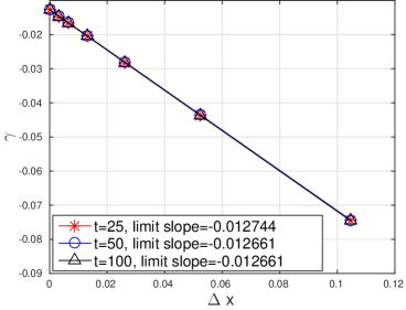
(a) Landau damping rate $\gamma$

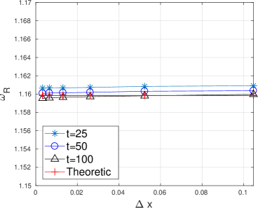
(b) Landau damping frequency $\omega_{R}$

Figure 6: Profile of the numerical damping rates and the numerical frequencies with respect to the space grid step $\Delta x$ with $k=0.3$ and $M=50$. The total evolution time is $t=25,50$ and $100$ respectively. The damping rate $\gamma$ in (a) is obtained by the least square fitting of the damping rate with different $\Delta x$. The intercept of the line on $y$-axis is the limit damping rate. The frequency $\omega_{R}$ of the electric field in (b) is estimated by counting the peaks in Figure 5.

Damping rate and frequency

As argued in Section 3.2.1 and 3.2.2, the filtered HME is a solver of VP, so the filtered HME would predict the correct Landau damping rate and frequencies if the moment order $M$ is large enough. To study it, we first study the spatial convergence to avoid the effects of the spatial error to the moment convergence and then study the moment convergence.

Spatial convergence

Figure 5 presents detailed illustrations of the evolution of $\mathcal{E}(t)$ with different grid sizes as $N=200$, $400$, $800$, $1600$, and $3200$. As the grid number increasing, the damping rate converges. The least square fitting method used in [10] is utilized here to approximate the final damping rate. The analytical solution of Landau damping rate and frequency for $k=0.3$ is

$$\omega_{R}=1.1598,\quad\gamma=-0.0126.$$ (52)

Figure 6(a) presents the damping rates for different spatial grid steps and different total evolution time. The numerical damping rates are in a linearly and monotonically converging pattern with the spatial grid size $\Delta x$ going to zero and the limit slope we obtained is in perfect agreement with the theoretical data. The Landau damping frequencies in Figure 6(b) also has a good convergence to the theoretical results with the increasing of spatial grids.

Moreover, the damping rates and frequencies for different end time $t_{end}$ are also studied. Three end time $t_{end}=25$, $50$ and $100$ correspond to the cases before the recurrence, just after the recurrence and a long time after the recurrence of HME. Figure 6(a) shows that the damping rates before and after the recurrence of the HME are almost same, while Figure 6(b) shows that the frequencies before and after the recurrence of the HME are just slightly different. This indicates that the filtered HME can predict the correct damping rate and frequency for a long time after the recurrence of HME.

Moment convergence

Figure 7(a) presents the time evolution of $\mathcal{E}(t)$ of the filtered HME for different moment order $M=40$, $50$, $60$, $70$ and $80$ with $k=0.3$, $N=3200$. One can observe that the behavior of the time evolution of $\mathcal{E}(t)$ for different numbers of moments are all persisting on damping. This indicates that the filter works well with different numbers of moments.

\psfrag{E}{\footnotesize$\mathcal{E}$}\includegraphics[width=115.23547pt]{k_03N_3200M_50_moment_c.eps}

(a) Moment Convergence

\psfrag{E}{\footnotesize$\mathcal{E}$}\includegraphics[width=115.23547pt]{slope_k_03N_3200_c.eps}

(b) Damping rate $\gamma$

\psfrag{E}{\footnotesize$\mathcal{E}$}\includegraphics[width=115.23547pt]{k_03N_3200_aveperiod_c.eps}

(c) Damping frequency $\omega_{R}$

Figure 7: (a) Time evolution of $\ln(\mathcal{E}(t))$ for different $M$ with $N=3200$, $k=0.3$. (b), (c) Numerical Landau damping rates and numerical Landau damping frequencies for different $M$ with $k=0.3$, $N=3200$ and different total evolution time, respectively.

The damping rates and frequencies for different end time $t_{end}$ are also studied. Three end time $t_{end}=25$, $50$ and $100$ is studied, and results are presented in Figure 7(b) and 7(c). It is clear that the damping rates at different ending time are almost the same and they are converging with the increasing of moment number. Because of the spatial error, there is a little distance between theoretical damping rate and the converging limit. But as it is stated in 4.2.1, the distance will go to zero with the increasing of the spatial grid size. Meanwhile, one can observe that the damping frequencies for different ending time are just slightly different. Moreover, with different numbers of moments, the frequencies are almost same. This indicates that the filtered HME can predict the correct damping rate and frequency with a small number of moments.

Conservation property

It has been proved in [10] that the numerical scheme used in this paper preserved the conservation of total mass and momentum, expect the total energy. We study the time evolution of the variation of the total energy, which is presented in Figure 8 for the setup $N=3200$, $M=50$ and $k=0.3$. It is clear that the total energy changes very slightly in the whole computation, which agrees with the result in [10]. This indicates the filter does not deteriorate the conservation of the mass, momentum and energy.

\psfrag{en}{\footnotesize{$\>\mathcal{E}$}}\psfrag{varivation}{relative variation}\includegraphics[width=192.0548pt,height=142.26378pt]{k_03N_3200M_50_error_c.eps}

Figure 8: Time evolution of the relative variation of the total energy $\mathcal{E}_{total}(t)$ in logarithm scale. The relative variation is defined by $|\mathcal{E}_{total}(t)-\mathcal{E}_{total}(0)|/\mathcal{E}_{total}(0)$.

4.2.2 2D-2D example

In this subsection, we study the filtered HME by 2D linear Landau damping and try to claim that all the conclusions for 1D case also hold for the 2D case. In the following, we pick up a few behaviors studied for 1D case to validate our conclusion. The initial value in [24] is adopted here:

$$f(0,x,y,v_{x},v_{y})=f_{eq}=\frac{1}{2\pi}\exp\left(-\frac{v_{x}^{2}+v_{y}^{2}}{2}\right)\Big{(}1+A\cos(k_{x}x)\cos(k_{y}y)\Big{)},$$ (53)

with $A=10^{-3}$ and $k_{x}=k_{y}=0.3$. The length of the periodic box in the physical space is $L_{x}=L_{y}=4\pi/k_{x}$. The moment order is set as $M=40$.

Figure. 9(a) presents the time evolution of the electric energy $\mathcal{E}(t)$ of HME and the filtered HME. Just similar to the 1D case, $\mathcal{E}(t)$ for the filtered HME keeps on damping at the time when the recurrence occurs for HME. Figure 9(b) shows the convergence of the damping rate with the increasing of grid number, where the grid number are $N=100$, $200$, $300$ and $400$, respectively.

Remark 2.

The difference between the numerical result and the theoretical result may be caused by the smaller $N$ and not large enough moment order $M$, which is restricted by the computational cost. Maybe the second order scheme we are working on can solve this problem.

Figure 9(c) illustrates the relative error of the total energy with the time evolution for the 2D-2D case with the setup $N_{x}=N_{y}=100$, $M=40$ and $k=0.3$. Same as the 1D case, the total energy is changing very slightly in the whole computation, which is due to the splitting numerical method.

\begin{overpic}[height=99.58464pt]{2d_x_c.eps} \end{overpic}

(a) Filter effect

\begin{overpic}[height=99.58464pt]{2d_total_c.eps} \end{overpic}

(b) Landau damping

\begin{overpic}[height=99.58464pt]{2d_error_c.eps} \end{overpic}

(c) Conservation

Figure 9: (a) Time evolution of $\ln(\mathcal{E}(t))$ for HME and the filtered HME with $N_{x}=N_{y}=200$ and $M=40$. (b) Time evolution of $\ln(\mathcal{E}(t))$ for the filtered HME with $M=40$ for different grid sizes. (c) Relative variation of the total energy.

4.3 Two-stream instability

In this subsection, the classical two-stream instability problem is employed to study the filtered HME. The two-stream instability is excited when the distribution function is formed by two populations streaming in opposite directions with a large enough relative drift velocity. Here, we adopt the same initial condition as in [12]

$$f(0,x,v)=\frac{1+\epsilon\cos(kx)}{2\sqrt{2\pi}}\left(\exp\left(-\left(\frac{v+u_{0}}{\sqrt{2}u_{th}}\right)^{2}\right)+\exp\left(-\left(\frac{v-u_{0}}{\sqrt{2}u_{th}}\right)^{2}\right)\right),$$ (54)

where the wave number $k=0.5$, perturbation $\epsilon=10^{-3}$, velocity $u_{0}=1.0$, and thermal velocity $u_{th}=0.5$ respectively.

Figure 10 depicts the time evolution of the electric energy $\mathcal{E}(t)$, where the reference solution is computed by the discrete velocity method (DVM) with the grid size large enough. Figure 10(a) shows the convergence of the electric energy with respect to the grid size with $M=60$. This indicates the filtered HME can depict the two-stream instability problem. Figure 10(b) presents the time evolution of the electric energy of HME and the filtered HME and also compare them with the reference solution. One can see the good agreement with the solution of DVM and reference theoretical rate. Moreover, the filtered HME behaviors better than HME for this problem. Good agreement with the reference shows the power of the filtered HME, saying this method is designed to suppress the numerical recurrence, but it also works for the nonlinear two-steam instability problem.

\begin{overpic}[height=142.26378pt]{two_stream_convergence_c.eps} \end{overpic}

(a) Spatial convergence

\begin{overpic}[height=142.26378pt]{two_stream_filter_c.eps} \end{overpic}

(b) With or without filter

Figure 10: (a) Time evolution of $\ln(\mathcal{E}(t))$ of the filtered HME for different spatial grid sizes with $M=60$. (b) Time evolution of $\ln(\mathcal{E}(t))$ of HME and the filtered HME and comparison with reference solution.

Figure 11 illustrates the time evolution of the relative error of the total energy. The setup is $N=3200$ and $M=60$. It is shown that the total energy is changing very slightly in the whole computation, and the variations of the total energy in the nonlinear stage is also acceptable, since this is quite a complicate physical process.

\psfrag{en}{\footnotesize{$\>\mathcal{E}$}}\psfrag{variation}{relative variation}\includegraphics[width=192.0548pt,height=142.26378pt]{two_error_c.eps}

Figure 11: Time evolution of the relative variation of the total energy $\mathcal{E}_{total}(t)$ for two-stream instability problem.

5 Conclusion

We presented a filtered HME for the Vlasov-Poisson equations to suppress the recurrence effects. Due to the careful construction, the filter preserves most of physical properties of HME, including the conservation of mass, momentum and energy, Galilean invariant and convergence to VP. The quasi time-consistent property guarantees that the solution to the filtered HME is not sensitive to the time step. Two viewpoints on the quasi time-consistent filter show that the filtered HME is a solver of the Vlasov equation, and it can predict correct physical phenomena described by VP. Numerical simulations demonstrate the power of the filter in suppressing recurrences and producing more accurate solutions. The proposed numerical method can depict the electric energy until it is close to the machine precision for linear Landau damping cases and predict correct behaviors of the electric energy for two-stream instability problem. More applications of the filtered HME are in process.

References

- [1] S. Adjerid and J. E. Flaherty. A moving finite element method with error estimation and refinement for one-dimensional time dependent partial differential equations. SIAM J. Numer. Anal., 23(4):778–796, 1986.
- [2] T. P. Armstrong. Numerical studies of the nonlinear Vlasov equation. Phys. Fluids, 10:1269–1280, 1967.
- [3] T. P. Armstrong, R. C. Harding, G. Knorr, and D. Montgomery. Solution of Vlasov’s equation by transform methods. J. Sci. Comput., 9:29–86, 1970.
- [4] P. L. Bhatnagar, E. P. Gross, and M. Krook. A model for collision processes in gases. I. small amplitude processes in charged and neutral one-component systems. Phys. Rev., 94(3):511–525, 1954.
- [5] Charles K Birdsall and A Bruce Langdon. Plasma physics via computer simulation. McGraw-Hill, NewYork, 2004.
- [6] S. L. Bourdiec, F. D. Vuyst, and L. Jacquet. Numerical solution of the vlasov–poisson system using generalized hermite functions. Commun. Comput. Phys., 175(8):528–544, 2006.
- [7] Z. Cai, Y. Fan, and R. Li. Globally hyperbolic regularization of Grad’s moment system. Comm. Pure Appl. Math., 67(3):464–518, 2014.
- [8] Z. Cai, Y. Fan, and R. Li. From discrete velocity model to moment method. Mathematica Numerica Sinica, 38(3):227–244, 2016.
- [9] Z. Cai, Y. Fan, R. Li, T. Lu, and Y. Wang. Quantum hydrodynamic model by moment closure of wigner equation. J. Math. Phys., 53(10):103503, 2012.
- [10] Z. Cai, R. Li, and Y. Wang. Solving Vlasov equation using NR method. SIAM J. Sci. Comput., 35(6):A2807–A2831, 2013.
- [11] Z. Cai and Y. Wang. Suppression of recurrence in the Hermite-spectral method for transport equations. preprint, 2017.
- [12] E. Camporeale, G. L. Delzanno, B. K. Bergen, and J. D. Moulton. On the velocity space discretization for the Vlasov-Poisson system: Comparison between implicit Hermite spectral and Particle-in-Cell methods. Commun. Comput. Phys., 198:47–58, 2016.
- [13] C. Canuto, M. Y. Hussaini, A. M. Quarteroni, A. Thomas Jr, et al. Spectral methods in fluid dynamics. Springer Science & Business Media, 2012.
- [14] J. Carrillo, M. Gamba, A. Majorana, and C. Shu. A weno-solver for the transients of boltzmann-poisson system for semiconductor devices. performance and comparisons with monte carlo methods. J. Comput. Phys., 184:498–525, 2003.
- [15] C. Z. Cheng and G. Knorr. The integration of the Vlasov equation in configuration space. J. Comput. Phys., 22:330–351, 1976.
- [16] Y. Cheng, M. Gamba, and J. Morrison. Study of conservation and recurrence of runge-kutta discontinuous galerkin schemes for vlasov-poisson systems. J. Sci. Comput., 56:319–349, 2013.
- [17] N. Crouseilles and F. Filbet. Numerical approximation of collisional plasmas by high order methods. J. Comput. Phys., 201(2):546–572, 2004.
- [18] Y. Di, Z. Kou, and R. Li. High order moment closure for Vlasov-Maxwell equations. Front. Math. China, 10(5):1087–1100, 2015.
- [19] Bengt Eliasson. Numerical simulations of the fourier-transformed vlasov-maxwell system in higher dimensions—theory and applications. Transport Theory and Statistical Physics, 39(5-7):387–465, 2010.
- [20] B. Ellasson. Outflow boundary conditions for Fourier transformed one-dimensional Vlasov-Poisson system. J. Sci. Comput., 16:1–28, 2001.
- [21] E. Fatemi and F. Odeh. Upwind finite difference solution of boltzmann equation applied to electron transport in semiconductor devices. J. Comput. Phys., 108(2):209 – 217, 1993.
- [22] F. Filbet. Convergence of a finite volume scheme for the vlasov–poisson system. SIAM J. Numer. Anal., 39(4):1146–1169, 2001.
- [23] F. Filbet and E. Sonnendrücker. Comparison of Eulerian Vlasov solvers. Comput. Phys. Comm., 150(3):247–266, 2003.
- [24] F. Filbet, E. Sonnendrücker, and P. Bertrand. Conservative numerical schemes for the Vlasov equation. J. Comput. Phys., 172:166–187, 2001.
- [25] D. Gottlieb and J. S. Hesthaven. Spectral methods for hyperbolic problems. J. Comput. Appl. Math., 128:83–131, 2001.
- [26] H. Grad. On the kinetic theory of rarefied gases. Comm. Pure Appl. Math., 2(4):331–407, 1949.
- [27] F. C. Grant and M. R. Feix. Fourier-Hermite solutions of the Vlasov equations in the linearized limit. Phy. Fluids, 10(4):696–702, 1967.
- [28] R. E. Heath, I. M. Gamba, P. J. Morrison, and C. Michler. A discontinuous Galerkin method for the Vlasov-Poisson system. J. Comput. Phys., 231(4):1140–1174, 2012.
- [29] J. S. Hesthaven and R. Kirby. Filtering in Legendre spectral methods. Math. Comput., 77(263):1425–1452, 2008.
- [30] J. P. Holloway. Spectral velocity discretizations for the Vlasov-Maxwell equations. Transport. Theor. Stat., 25(1):1–32, 1996.
- [31] T. Hou and R. Li. Computing nearly singular solutions using pseudo-spectral methods. J. Comput. Phys., 226(1):379–397, 2007.
- [32] G. Joyce, G. Knorr, and H. K. Meier. Numerical integration methods of the Vlasov equation. J. Comput. Phys., 8(1):53–63, 1971.
- [33] A. Kanevsky, K. Carpenter, and J. S. Hesthaven. Idempotent filtering in spectral and spectral element methods. J. Comput. Phys, 220(1):41 – 58, 2006.
- [34] A. J. Klimas. A method for overcoming the velocity space filamentation problem in collisionless plasma model solutions. J. Comput. Phys., 68(1):202–226, 1987.
- [35] A. J. Klimas and W. M. Farrell. A splitting algorithm for Vlasov simulation with filamentation filtration. J. Comput. Phys., 110(1):150–163, 1994.
- [36] H.O. Kreiss and J. Oliger. Stability of the Fourier method. SIAM J. Numer. Anal., 16:421 – 433, 1979.
- [37] L. Landau. On the vibrations of the electronic plasma. Eur. J. Org. Chem., 2006(2):498–506, 1946.
- [38] R. G. McClarren and C. D. Hauck. Robust and accurate filtered spherical harmonics expansions for radiative transfer. J. Comput. Phys., 229(16):5597–5614, 2010.
- [39] I. Müller and T. Ruggeri. Rational Extended Thermodynamics, Second Edition, volume 37 of Springer tracts in natural philosophy. Springer-Verlag, New York, 1998.
- [40] C. S. Ng, A. Bhattacharjee, and F. Skiff. Complete spectrum of kinetic eigenmodes for plasma oscillations in a weakly collisional plasma. Phys. Rev. Lett., 92(6):065002, 2004.
- [41] J. T. Parker and P. J. Dellar. Fourier-Hermite spectral representation for the Vlasov-Poisson system in the weakly collisional limit. J. Plasma. Phys., 81(02):305810203, 2015.
- [42] J. Qiu and C. Shu. Positivity preserving semi-Lagrangian discontinuous Galerkin formulation: Theoretical analysis and application to the Vlasov-Poisson system. J. Comput. Phys., 230(23):8386 – 8409, 2011.
- [43] J. W. Schumer and J. P. Holloway. Vlasov simulation using velocity-scaled Hermite representations. J. Comput. Phys., 144(2):626–661, 1998.
- [44] M. Shoucri and G. Knorr. Numerical integration of the vlasov equation ☆. J. Comput. Phys., 14(1):84–92, 1974.
- [45] E. Sonnendrücker, J. Roche, P. Betrand, and A. Ghizzo. The semi-Lagrangian method for the numerical resolution of Vlasov equations. J.Comput. Phys, 149(2):201–220, 1998.
- [46] M. Torrilhon. Two dimensional bulk microflow simulations based on regularized Grad’s 13-moment equations. SIAM Multiscale. Model. Simul., 5(3):695–728, 2006.
- [47] A. A. Vlasov. On vibration properties of electron gas. J. Exp. Theor. Phys., 8(3):291, 1938.
- [48] S. I. Zaki, R. T. Gardner, and T. J. Boyd. A finite element code for the simulation of one-dimensional Vlasov plasmas. i. Theory. J. Comput. Phys., 79:184–199, 1988.