Time-Space Trade-Offs for Computing Euclidean Minimum Spanning Trees

Abstract

We present time-space trade-offs for computing the Euclidean minimum spanning tree of a set $S$ of $n$ point-sites in the plane. More precisely, we assume that $S$ resides in a random-access memory that can only be read. The edges of the Euclidean minimum spanning tree $\operatorname{EMST}(S)$ have to be reported sequentially, and they cannot be accessed or modified afterwards. There is a parameter $s\in\{1,\dots,n\}$ so that the algorithm may use $O(s)$ cells of read-write memory (called the workspace) for its computations. Our goal is to find an algorithm that has the best possible running time for any given $s$ between $1$ and $n$.

We show how to compute $\operatorname{EMST}(S)$ in $O\big{(}(n^{3}/s^{2})\log s\big{)}$ time with $O(s)$ cells of workspace, giving a smooth trade-off between the two best known bounds $O(n^{3})$ for $s=1$ and $O(n\log n)$ for $s=n$. For this, we run Kruskal’s algorithm on the relative neighborhood graph (RNG) of $S$. It is a classic fact that the minimum spanning tree of $\operatorname{RNG}(S)$ is exactly $\operatorname{EMST}(S)$. To implement Kruskal’s algorithm with $O(s)$ cells of workspace, we define $s$-nets, a compact representation of planar graphs. This allows us to efficiently maintain and update the components of the current minimum spanning forest as the edges are being inserted.

1 Introduction

Given a set $S$ of $n$ point-sites in the plane, the Euclidean minimum spanning tree of $S$, $\operatorname{EMST}(S)$, is the minimum spanning tree of the complete graph with vertex set $S$, where the weight of an edge between two point-sites is the Euclidean distance between them. The problem of computing $\operatorname{EMST}(S)$ efficiently constitutes a core question of computational geometry, and it is discussed in virtually every introductory course on the subject. There are several algorithms that find $\operatorname{EMST}(S)$ in $O(n\log n)$ time and with $O(n)$ cells of space [12, 25].

Here, our goal is to design algorithms to compute $\operatorname{EMST}(S)$ in the limited-workspace model, where only a limited number of memory cells are available for reading and writing during the execution of the algorithm [8]. This model is of interest theoretically because it provides a trade-off between the running time and the space usage of an algorithm. It is also useful from a practical point of view, in developing software for portable devices and sensors where memory is the limiting factor. A significant amount of research has focused on the design of algorithms under memory constraints. Much of this work dates from the 1970s, when memory was an expensive commodity. Even today, while this cost has dropped substantially, at the same time the amount of data has increased, and the size of some devices has been reduced dramatically. In particular, sensors and small devices, where larger memories are neither possible nor desirable, have proliferated in recent years. Moreover, even if a device is equipped with a large memory, it may still be preferable to limit the number of write operations. For example, writing to flash memory is slow, and it may reduce the lifetime of the memory. Additionally, if the input is stored on removable devices, write-access may not be allowed due to technical or security concerns.

There are many variants of the limited-workspace model [8], but the general outline is usually the same: the input resides in a read-only memory and cannot be modified directly by the algorithm. Instead, the algorithm may use a controlled amount of storage cells (usually called workspace) that reside in a local memory and can be modified as needed to solve the problem. Since the result of the computation may not fit in the local memory, the model provides a write-only memory where the output is reported sequentially. One noteworthy instance of the model is encountered in computational complexity theory, where the complexity class LOGSPACE consists of all decision problems that can be solved with a deterministic Turing machine that has access to two tapes [3]. The first tape is read-only and contains the input, while the second tape represents the workspace and contains a logarithmic (in the input size) number of read-write bits. In other words, the second tape stores only a constant number of words with a logarithmic number of bits that can be used as counters or as pointers to the input. Thus, the computational model represented by LOGSPACE is sometimes referred to as the constant-workspace model [6, 5].

More generally, we may allow the algorithm to use a workspace of $O(s)$ cells, for some parameter $s$, where a cell stores either an input item (such as a point coordinate), a pointer into the input structure (of logarithmic size in the input length), or a counter (with a logarithmic number of bits). The goal is to design algorithms whose running time decreases as $s$ increases, and to obtain a smooth trade-off between workspace size and running time.

Our results.

For computing the Euclidean minimum spanning tree of $n$ given point-sites in the plane in the constant-workspace model, Asano et al. [5] presented an algorithm that runs in $O(n^{3})$ time. We use their method as a starting point for a time-space trade-off. As a result, we obtain an algorithm that, for any given number $s\in\{1,\dots,n\}$ of workspace cells, computes the EMST in $O\big{(}(n^{3}/s^{2})\log s\big{)}$ time. This yields a smooth transition between the $O(n^{3})$ time algorithm for $s=1$ by Asano et al. [5] and the classic $O(n\log n)$ algorithm for $s=n$ [12, 25].

As a main tool, we define a compact representation of a plane graph $G$, called the $s$-net. The $s$-net consists of a “dense” set of $s$ edges in $G$ for which we remember the edge-face incidences. That is, for each edge $e$ in the $s$-net, we store the (at most two) faces of $G$ to which $e$ is incident. Furthermore, for each face in $G$ that has at least one incident edge in the $s$-net, we store the order in which the incident edges of the $s$-net appear. The density property guarantees that we cannot walk for more than $O(s)$ steps along a connected component of the boundary of a face in $G$ without reaching an edge of the $s$-net. This turns out to be useful for an efficient limited-workspace implementation of Kruskal’s MST-algorithm on a plane graph $G$. Recall that in this algorithm, the edges of $G$ are inserted into an auxiliary graph by increasing order of weight. To insert a new edge $e$, we need to determine whether the endpoints of $e$ are in the same component of the current auxiliary graph. If $G$ is plane, this amounts to testing whether the endpoints of $e$ are incident to the same face of the current auxiliary graph—precisely the task for which $s$-nets were created. While the $s$-net is designed to speed up Kruskal’s algorithm, this structure may be of independent interest, as it provides a compact way to represent plane graphs that may be useful in other problems.

Related work.

The study of constant-workspace algorithms in theoretical computer science started with the complexity class LOGSPACE [3]. Since then, many classic problems were considered in this setting. For example, there are a lot of relevant results on selection and sorting [22, 23, 24, 14]. A long-standing algorithmic problem in graph theory was eventually solved by Reingold [26], who showed that the reachability between two vertices in an undirected graph can be decided in LOGSPACE. The model was made popular in computational geometry by Asano et al. [5], who presented several algorithms to compute classic geometric structures in the constant-workspace model (see the recent survey [8]). Time-space trade-offs for many of these structures were presented in subsequent years [4, 10, 20, 9, 7, 2, 11, 16, 18, 1, 17], with the notable exception of the EMST. This is finally addressed here.

2 Preliminaries and Notation

We recall the basic definition and some properties of the Euclidean minimum spanning tree, and we briefly review some known algorithms for computing it, both in the classic setting and in the constant-workspace model. Furthermore, we recall the definition of the relative neighborhood graph (RNG), a basic proximity structure defined on planar point sets, and we discuss the relationship between RNGs and Euclidean minimum spanning trees.

2.1 Euclidean Minimum Spanning Trees

Let $S=\{p_{1},\dots,p_{n}\}\subset\mathbb{R}^{2}$ be a set of $n$ point-sites in the plane, from now on referred to as sites. We assume that $S$ is in general position, i.e., no three sites lie on a common line, no four sites lie on a common circle, and the pairwise distances between the sites are all distinct. Let $G_{S}$ be the complete weighted graph with vertex set $S$, where the edges are weighted with the Euclidean distance between their endpoints. A minimum spanning tree of $G_{S}$ is called a Euclidean minimum spanning tree of $S$, and it is denoted by $\operatorname{EMST}(S)$, see Figure 1.

(a)

(b)

Figure 1: A set $S$ of sites in the plane, and (a) a spanning tree of the complete graph with vertex set $S$ and (b) the Euclidean minimum spanning tree of $S$.

Under our general position assumption, it is known that $\operatorname{EMST}(S)$ is unique (see, e.g., [15]). Given $S$, we would like to report the edges of $\operatorname{EMST}(S)$ in any order, so that each edge is listed exactly once.

A Classic Algorithm.

We recall the classic algorithm by Kruskal [15]: we start with an empty forest $F$, and we consider the edges of $G_{S}$ one by one, by increasing weight. In each step, we insert the current edge $e$ into $F$ if and only if there is no path in $F$ between the endpoints of $e$; see Figure 2. After all edges of $G_{S}$ have been considered, the final graph $F$ is exactly $\operatorname{EMST}(S)$.

(a)

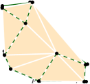
(b)

Figure 2: Two steps in Kruskal’s algorithm for computing the EMST for a set of sites in the plane. (a) In this step, the algorithm adds $e_{1}$ to $F$, since there is no path between $p$ and $q$ in $F$. (b) In the next step, $e_{2}$ is discarded, since $q$ and $r$ lie in the same component of $F$.

During the above procedure, using a disjoint set-union structure, we keep track of the components of $F$ so that we can determine if there is a path in $F$ between the two endpoints of the next edge $e$ [15]. With an efficient implementation of the disjoint set-union structure, the time for inserting the edges into $F$ is dominated by the time for sorting the edges with their weight. This gives a running time of $O(n^{2}\log n)$ with $O(n)$ cells of workspace.

The running time can be improved as follows: the Delaunay triangulation of $S$, $\operatorname{DT}(S)$, is the triangulation of $S$ in which three sites $p,q,r$ form a triangle if and only if the disk with $p$, $q$, and $r$ on the boundary contains no other sites from $S$ in its interior [12]. Under our general position assumption, this defines a unique plane triangulation of $S$ which is a supergraph of $\operatorname{EMST}(S)$; see Figure 3 [12]. Thus, $\operatorname{EMST}(S)$ is the minimum spanning tree of $\operatorname{DT}(S)$, and it suffices to consider the $O(n)$ edges of $\operatorname{DT}(S)$ instead of the $O(n^{2})$ edges of $G_{S}$. Then, Kruskal’s algorithm runs in $O(n\log n)$ time, when $O(n)$ cells of workspace are available [12].

Figure 3: The Delaunay triangulation $\operatorname{DT}(S)$ and the Euclidean minimum spanning tree $\operatorname{EMST}(S)$ for a planar point set $S$. The dashed edges belong to $\operatorname{EMST}(S)$.

The Constant-Workspace Algorithm.

Asano et al. [5] presented an algorithm that reports the edges of $\operatorname{EMST}(S)$ in $O(n^{3})$ time with $O(1)$ cells of workspace. Like the classic method, their algorithm uses the fact that $\operatorname{EMST}(S)$ is a subgraph of $\operatorname{DT}(S)$. First, Asano et al. show that there exists a constant-workspace algorithm that solves the following task in $O(n)$ time: given an edge $pq$ of $\operatorname{DT}(S)$, find the next edge $pr$ of $\operatorname{DT}(S)$ that is incident to $p$ after $pq$ in clockwise direction. Using the fact that for each $p\in S$, the edge between $p$ and its nearest neighbor in $S\setminus\{p\}$ belongs to $\operatorname{DT}(S)$, this gives an algorithm that reports the edges of $\operatorname{DT}(S)$, one by one, in an arbitrary order, in $O(n)$ time per edge. We will not describe the details here, but we present an analogous result for relative neighborhood graphs in Section 3.

Then, the algorithm of Asano et al. to list the edges of $\operatorname{EMST}(S)$ proceeds as follows: we run the constant-workspace algorithm that enumerates the edges of $\operatorname{DT}(S)$. Every time a new edge $e$ of $\operatorname{DT}(S)$ is reported, we test if $e$ is in $\operatorname{EMST}(S)$. If so, we output $e$; otherwise, we discard it. To perform this test, we consider the subgraph $\operatorname{DT}_{<e}$ of $\operatorname{DT}(S)$ that contains all the edges of length less than $|e|$, where $|e|$ denotes the (Euclidean) length of $e$. By the cut-property of minimum spanning trees, it follows that $e$ is not in $\operatorname{EMST}(S)$ if and only if the endpoints $p$ and $q$ of $e$ lie in the same connected component of $\operatorname{DT}_{<e}$. Since $\operatorname{DT}(S)$ is plane, this means that $e$ is not in $\operatorname{EMST}(S)$ if and only if $p$ and $q$ lie on a common connected component of the boundary of the face of $\operatorname{DT}_{<e}$ that contains $e$. In other words, $e\notin\operatorname{EMST}(S)$ if and only if we encounter $q$ by walking from $p$ along the connected component of the boundary of the face of $\operatorname{DT}_{<e}$ that contains $e$; see Figure 4.

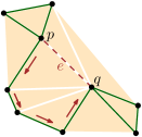
Figure 4: The subgraph $\operatorname{DT}_{<e}$ for a planar point set $S$ and an edge $e=pq$ of $\operatorname{DT}(S)$. To decide if $e$ belongs to $\operatorname{EMST}(S)$, we check if $p$ to $q$ are in the same connected component of $\operatorname{DT}_{<e}$. For this, we walk along the boundary of the face of $\operatorname{DT}_{<e}$ that contains $e$, starting from $p$.

To perform one step of this walk, we use the above-mentioned subroutine due to Asano et al. that receives an edge of $\operatorname{DT}(S)$ and finds the next clockwise edge of $\operatorname{DT}(S)$ using $O(n)$ time and $O(1)$ cells of workspace. We start with the edge $e=pq$ and we repeatedly call the subroutine until we find the first Delaunay edge $pr$ of length less than $|e|$ (if no such edge exists, then $e$ belongs to $\operatorname{EMST}(S)$). Then, we repeatedly call the subroutine, starting with the reverse edge $rp$, until we encounter an edge $rs$ with length less than $|e|$. We continue until either (i) we encounter $q$, in which case $e$ does not belong to $\operatorname{EMST}(S)$; or (ii) the subroutine produces the edge $e$, which means that we have traversed the complete connected component of the face boundary without seeing $q$, in which case $e$ belongs to $\operatorname{EMST}(S)$. During this walk, each edge of $\operatorname{DT}(S)$ is generated at most twice, at most once for each endpoint. Thus, we need $O(n^{2})$ time to decide if an edge $e$ of $\operatorname{DT}(S)$ is in $\operatorname{EMST}(S)$, with $O(1)$ cells of workspace.

Since $\operatorname{DT}(S)$ has $O(n)$ edges, and since it takes $O(n^{2})$ time to decide membership in $\operatorname{EMST}(S)$, the total time to find all the edges of $\operatorname{EMST}(S)$ is $O(n^{3})$. The overhead for computing the edges of $\operatorname{DT}(S)$ in the outer loop is $O(n^{2})$, which is negligible compared to the remainder of the algorithm. The workspace is constant. We can also report the edges of $\operatorname{EMST}(S)$ by increasing length: we repeatedly list all edges of $\operatorname{DT}(S)$, and each time we find the shortest edge $e\in\operatorname{DT}(S)$ whose membership in $\operatorname{EMST}(S)$ has not yet been checked, we apply our test to $e$. Now, the overhead for the outer loop is $O(n^{3})$ instead of $O(n^{2})$, without any effect on the total asymptotic running time.

2.2 Relative Neighborhood Graphs

The relative neighborhood graph is a geometric structure that “lies between” the Euclidean minimum spanning tree and the Delaunay triangulation. For two sites $p,q\in S$, we define the lens of $p$ and $q$ as the intersection of the disk centered at $p$ with radius $|pq|$ and the disk centered at $q$ with radius $|pq|$, where $|\cdot|$ denotes the Euclidean distance. The lens of $p$ and $q$ is called empty if it contains no sites of $S\setminus\{p,q\}$ in its interior. In other words, the two sites $p$ and $q$ have the empty lens property if there is no site $r\in S\setminus\{p,q\}$ such that both $|pr|$ and $|qr|$ are shorter than $|pq|$; see Figure 5.

Figure 5: A set $S$ of sites and two sites $p,q\in S$. The disks $D_{p}$ and $D_{q}$ have radius $|pq|$ and are centered at $p$ and $q$, respectively. The two sites $p$ and $q$ satisfy the empty lens property since $D_{p}\cap D_{q}$ is empty of other sites of $S$.

The relative neighborhood graph $\operatorname{RNG}(S)$ of $S$ is the undirected graph with vertex set $S$ obtained by connecting two sites $p,q\in S$ with an edge if and only if the lens of $p$ and $q$ is empty [27]. One can show that a plane embedding of $\operatorname{RNG}(S)$ is obtained by drawing the edges as straight line segments between the corresponding sites in $S$; see Figure 6. By definition, $\operatorname{RNG}(S)$ is a subgraph of $\operatorname{DT}(S)$. Furthermore, it is well-known that $\operatorname{EMST}(S)$ is a subgraph of $\operatorname{RNG}(S)$ [12]. In particular, this implies that $\operatorname{RNG}(S)$ is connected; see Figure 7. Each vertex in $\operatorname{RNG}(S)$ has at most six neighbors, so $\operatorname{RNG}(S)$ has bounded degree and $O(n)$ edges. We will denote the number of those edges by $m$. Given $S$, we can list the edges of $\operatorname{RNG}(S)$ in $O(n\log n)$ time using $O(n)$ cells of workspace [27, 19, 21].

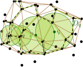
Figure 6: An edge $pq$ in $\operatorname{RNG}(S)$. The lens of $p$ and $q$ is empty.

Figure 7: An illustration of the fact $\operatorname{EMST}(S)\subseteq\operatorname{RNG}(S)\subseteq\operatorname{DT}(S)$. The dashed black edges belong to $\operatorname{EMST}(S)$ and are a subset of the green edges which represent $\operatorname{RNG}(S)$. All these edges form a subset of the edges of the underlying graph $\operatorname{DT}(S)$.

Thus, we can compute $\operatorname{EMST}(S)$ with the algorithm of Kruskal using the edges of $\operatorname{RNG}(S)$ instead of $\operatorname{DT}(S)$. Since both $\operatorname{RNG}(S)$ and $\operatorname{DT}(S)$ have $O(n)$ edges, this does not improve the running time of Kruskal’s algorithm in the classic setting where $O(n)$ cells of workspace are available. However, since $\operatorname{RNG}(S)$ (unlike $\operatorname{DT}(S)$) has bounded degree, it turns out to be the superior choice for the limited-workspace model.

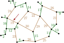
Figure 8: The $\operatorname{RNG}$ for a set $S$ of sites. The labels represent the indices of the edges in the sorted sequence $E_{R}$. The subgraph $\operatorname{RNG}_{19}$ is shown in green. The edge $e_{19}$ does not belong to $\operatorname{EMST}(S)$ since its endpoints lie in the same component of $\operatorname{RNG}_{19}$.

We define $E_{R}=e_{1},\dots,e_{m}$ to be the sorted sequence of edges in $\operatorname{RNG}(S)$, in increasing order of length. For $i\in\{1,\dots,m\}$, we define $\operatorname{RNG}_{i}$ to be the subgraph of $\operatorname{RNG}(S)$ with vertex set $S$ and edge set $\{e_{1},\dots,e_{i-1}\}$. Thus, to check if $e_{i}$ belongs to $\operatorname{EMST}(S)$, the algorithm by Kruskal checks if the endpoints of $e_{i}$ lie on the same component of $\operatorname{RNG}_{i}$; see Figure 8.

In our algorithms, we represent each edge $e_{i}\in E_{R}$ by two directed half-edges. The two half-edges are oriented in opposite directions such that the face incident to a half-edge lies on its left. We call the endpoints of a half-edge the head and the tail such that the half-edge is directed from the tail endpoint to the head endpoint. Furthermore, directed half-edges will be denoted as $\overrightarrow{e}$ and undirected edges as $e$; see Figure 9 for an illustration.

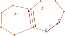
Figure 9: A schematic drawing of the faces $F,F^{\prime}$ of $\operatorname{RNG}(S)$. The two half-edges that correspond to the edge $e_{i}$ are oriented such that the face incident to each lies on its respective left. The sites $p$ and $q$ are the head and the tail endpoints of the half-edge $\overrightarrow{e_{j}}=\overrightarrow{pq}$, respectively.

Using the concept of half-edges, we define the face-cycle in a planar graph. For $i\in\{1,\dots,m\}$, a face-cycle in $\operatorname{RNG}_{i}$ is the circular sequence of consecutive half-edges such that (i) they bound either a face in $\operatorname{RNG}_{i}$ or the outer face in a connected component of $\operatorname{RNG}_{i}$; and (ii) every two consecutive half-edges $e$ and $e^{\prime}$ in a face-cycle share an endpoint which is the head vertex of $e$ and the tail of $e^{\prime}$.

The definition implies that all the half-edges in a face-cycle are oriented in the same direction and the face (or the outer face) incident to the half-edges lies on their left. Note that every half-edge lies on only one face-cycle; however, a site of $S$ might be on several face-cycles; see Figure 10. The partial relative neighborhood graph $\operatorname{RNG}_{i}$ can be represented as a collection of face-cycles.

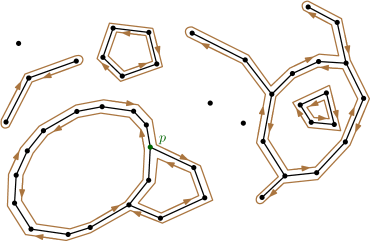
Figure 10: A schematic drawing of $\operatorname{RNG}_{i}$ for a planar set $S$ of sites. The edges are shown in black. The face-cycles of $\operatorname{RNG}_{i}$ are in beige. The half-edges of each face-cycle are directed according to the arrows on the corresponding cycle. The site $p\in S$ is on three face-cycles of $\operatorname{RNG}_{i}$. Each of the six half-edges incident to $p$ is only on one face-cycle.

Let $j\geq i\geq 1$. For a half-edge $\overrightarrow{e_{j}}$ with head $q$, we define the predecessor and the successor of $\overrightarrow{e_{j}}$ in $\operatorname{RNG}_{i}$ as follows: the predecessor $\text{pre}(\overrightarrow{e_{j}})$ of $\overrightarrow{e_{j}}$ is the half-edge in $\operatorname{RNG}_{i}$ which has $q$ as its head and is the first half-edge encountered in a counterclockwise sweep from $\overrightarrow{e_{j}}$ around $q$. The successor $\text{suc}(\overrightarrow{s_{j}})$ of $\overrightarrow{e_{j}}$ is the half-edge in $\operatorname{RNG}_{i}$ which has $q$ as its tail and is the first half-edge encountered in a clockwise sweep from $\overrightarrow{e_{j}}$ around $q$; see Figure 11 for an illustration. Note that, if there is no edge incident to $q$ in $\operatorname{RNG}_{i}$, we set both the predecessor and the successor to Null.

Let $i>j\geq 1$. For the half-edge $\overrightarrow{e_{j}}$ in $\operatorname{RNG}_{i}$ that lies on a face-cycle $F$, we define the next edge of $\overrightarrow{e_{j}}$ on $F$ as the half-edge on $F$ whose tail is the head of $\overrightarrow{e_{j}}$. Note that the next edge of a half-edge $\overrightarrow{e_{j}}$ is defined with respect to each diagram $\operatorname{RNG}_{i}$ with $i>j$ and thus $\overrightarrow{e_{j}}\in\operatorname{RNG}_{i}$, whereas the predecessor and successor of $\overrightarrow{e_{j}}$ are defined with respect to each diagram $\operatorname{RNG}_{i}$ with $i\leq j$, meaning that $\overrightarrow{e_{j}}\not\in\operatorname{RNG}_{i}$.

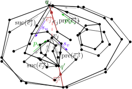
Figure 11: A schematic drawing of $\operatorname{RNG}_{i}$ and the half-edges $\overrightarrow{e_{j}}$ with head $q$ and $\overrightarrow{e_{j^{\prime}}}$ with head $q^{\prime}$, for $j,j^{\prime}\geq i\geq 1$. The predecessor and successor of $\overrightarrow{e_{j}}$ are $\text{pre}(\overrightarrow{e_{j}})$ and $\text{suc}(\overrightarrow{e_{j}})$, respectively. The predecessor and successor of $\overrightarrow{e_{j^{\prime}}}$ are $\text{pre}(\overrightarrow{e_{j^{\prime}}})$ and $\text{suc}(\overrightarrow{e_{j^{\prime}}})$, respectively.

3 Computing the Relative Neighborhood Graph

For the given set $S=\{p_{1},\dots,p_{n}\}$ of sites, our first goal is to compute the edges of $\operatorname{RNG}(S)$ in the limited-workspace model. We first present an algorithm for listing the edges of $\operatorname{RNG}(S)$ in an arbitrary order, using $O(s)$ cells of workspace. Then, we extend the algorithm so that it outputs the edges in sorted order according to their lengths. Our method is inspired by the time-space trade-off for Voronoi diagrams by Banyassady et al. [9].

3.1 All the Incident Edges to Some Sites

The idea is to subdivide $S$ into batches of $s$ sites, and to compute all the edges incident to the sites in one batch simultaneously. In the following lemma, we explain how to process one batch using $O(s)$ cells of workspace. This lemma is the main reason why we prefer to use $\operatorname{RNG}(S)$ instead of $\operatorname{DT}(S)$, the choice of Asano et al. [5]. More precisely, in $\operatorname{DT}(S)$, there may be sites of high degree, so that we cannot guarantee that all edges incident to the sites of a single batch can be found in the desired time.

Lemma 3.1.

Let $S$ be a planar set of $n$ point-sites in general position, stored in a read-only array. Given a set $Q\subseteq S$ of $s$ sites, we can compute for each $p\in Q$ the neighbors of $p$ in $\operatorname{RNG}(S)$ (for each $p$, there are at most six neighbors) in total time $O(n\log s)$ and using $O(s)$ cells of workspace.

Proof.

The algorithm has two phases. In the first phase, for each $p\in Q$, we find a set containing the neighbors of $p$ in $\operatorname{RNG}(S)$. This superset has size at most six. In the second phase, we check for each $p\in Q$ which of these candidate neighbors are the actual neighbors of $p$ in $\operatorname{RNG}(S)$.

The first phase proceeds in $\lceil n/s\rceil$ steps. In each step, we process a batch of $s$ sites of $S=R_{1}\cup\dots\cup R_{\lceil n/s\rceil}$, and we produce at most six candidate neighbors for each $p\in Q$. In the first step, we take the first batch $R_{1}\subseteq S$ of $s$ sites, and we compute $\operatorname{RNG}(Q\cup R_{1})$. Because $|Q\cup R_{1}|\leq 2s$, we can do this in $O(s\log s)$ time using known algorithms [27, 19, 21]. For each $p\in Q$, we remember the neighbors of $p$ in $\operatorname{RNG}(Q\cup R_{1})$ (there are at most six neighbors). Notice that if for a pair $p\in Q,r\in R_{1}$, the edge $pr$ is not in $\operatorname{RNG}(Q\cup R_{1})$, then the lens of $p$ and $r$ is non-empty. This also means that $pr$ is not an edge of $\operatorname{RNG}(S)$. Let $N_{1}$ be the set containing all neighbors in $\operatorname{RNG}(Q\cup R_{1})$ of all sites in $Q$. Storing $N_{1}$, the set of candidate neighbors, requires $O(s)$ cells of workspace.

Then, in each step $j=2,\dots,O(n/s)$, we take the next batch $R_{j}\subseteq S$ of $s$ sites, and we compute $\operatorname{RNG}(Q\cup R_{j}\cup N_{j-1})$ in $O(s\log s)$ time using $O(s)$ cells of workspace. For each $p\in Q$, we store the set of neighbors of $p$ in this computed graph (this set has size at most six). Additionally, we let $N_{j}$ be the set containing all neighbors in $\operatorname{RNG}(Q\cup R_{j}\cup N_{j-1})$ of all sites in $Q$. Note that $N_{j}$, the set of candidate neighbors, consists of $O(s)$ sites as each site in $Q$ has a degree of at most six in the computed graph. At this step, we do not need to store $N_{j-1}$ anymore.

After $\lceil n/s\rceil$ steps we are left with at most six candidate neighbors for each site in $Q$. As mentioned above, for a pair $p\in Q,r\in S$, if $r$ is not among the candidate neighbors of $p$, then, at some point in the construction, there was an obstructing site inside the lens of $p$ and $r$. Therefore, only the candidate neighbors can define edges of $\operatorname{RNG}(S)$, but not necessarily all of them. See Figure 12 for an example.

Figure 12: For $S=\{p_{1},\dots,p_{5}\}$, the set of neighbors of $p_{1}$ in $\operatorname{RNG}(S)$ is $\{p_{2},p_{3}\}$. Suppose that $p_{3}$ and $p_{4}$ are processed in some steps before $p_{5}$. After processing $p_{3}$ and $p_{4}$, the site $p_{4}$ is not a candidate neighbor of $p_{1}$, because $p_{3}$ lies in their lens. This results in $p_{5}$ becoming a candidate neighbor of $p_{1}$ in one of the following steps. Since $p_{4}$ is the only site in the lens of $p_{1}$ and $p_{5}$, the site $p_{5}$ will remain as a candidate neighbor of $p_{1}$.

In the second phase, to obtain the edges of $\operatorname{RNG}(S)$ incident to the sites in $Q$, we go again through the entire set $S=R_{1}\cup\dots\cup R_{\lceil n/s\rceil}$ in batches of size $s$: in the first step, we start with all the sites in $Q$ and their candidate neighbors in $N_{\lceil n/s\rceil}$, and we construct $\operatorname{RNG}(Q\cup R_{1}\cup N_{\lceil n/s\rceil})$. For each $p\in Q$ and for each candidate neighbor $r$ of $p$ in $N_{\lceil n/s\rceil}$, we check if $r$ is still a neighbor of $p$ in this computed graph. If not, we remove $r$ from the candidate neighbors of $p$. We denote the pruned set of candidate neighbors of all the sites in $Q$ by $N^{\prime}_{1}$. The candidate neighbors in $N_{\lceil n/s\rceil}$ for which there is an obstructing site in $R_{1}$ will not appear in $N^{\prime}_{1}$.

Then, in each step $j=2,\dots,O(n/s)$, we construct the graph $\operatorname{RNG}(Q\cup R_{1}\cup N^{\prime}_{j-1})$. Again, for each site $p\in Q$, we remove its candidate neighbors in $N^{\prime}_{j-1}$ that are no longer neighbors of $p$ in the computed graph. We denote the pruned set of candidate neighbors of all the sites in $Q$ by $N^{\prime}_{j}$. In this step, we do not need to store $N^{\prime}_{j-1}$ anymore. After going through all the batches, the candidates that have survived define the edges of $\operatorname{RNG}(S)$ incident to the sites in $Q$; see Figure 13. Note that in all the steps, $N^{\prime}_{j}$ contains at most six candidate neighbors for each site of $Q$, and thus, its size is $O(s)$.

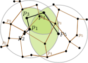
Figure 13: For a set of sites $S$ and $Q=\{p_{1},\dots,p_{5}\}$, the neighbors in $\operatorname{RNG}(S)$ of all the sites in $Q$ are generated.

Since the algorithm takes $O(s\log s)$ time per step, and since the number of steps is $2\cdot\lceil n/s\rceil$, the total running time of the algorithm is $O(n\log s)$. The space requirement for storing the candidate neighbors as well as the intermediate $\operatorname{RNG}$s is $O(s)$ cells of workspace. ∎

3.2 Finding All the Edges of RNG

Through repeated application of Lemma 3.1, we can compute all the edges of $\operatorname{RNG}(S)$, in some arbitrary order, using a workspace of $O(s)$ cells.

Theorem 3.2.

Suppose we are given a set of $n$ point-sites $S=\{p_{1},\dots,p_{n}\}$ in the plane in general position, stored in a read-only array. Let $s$ be a parameter in $\{1,\dots,n\}$. We can compute the edges of $\operatorname{RNG}(S)$ in total time $O\big{(}(n^{2}/s)\log s\big{)}$, using $O(s)$ cells of workspace.

Proof.

We take the set $Q$ of the first $s$ sites of $S$, and we apply Lemma 3.1 on $Q$ to find all the neighbors in $\operatorname{RNG}(S)$ of all the sites in $Q$. Whenever we find a neighbor $p_{j}$ of a site $p_{i}$ in $\operatorname{RNG}(S)$, we report the edge $p_{i}p_{j}$ only if $i<j$. This guarantees that the edge $p_{i}p_{j}$ of $\operatorname{RNG}(S)$ is reported only once. Then, we take the next batch of $s$ sites of $S$ and repeat the same procedure. We continue until all the sites in $S$ are processed, i.e., $O(n/s)$ times; see Figure 14.

Lemma 3.1 guarantees that all the reported edges belong to $\operatorname{RNG}(S)$ and all the edges of $\operatorname{RNG}(S)$ are reported exactly once. Regarding the running time of the algorithm, $O(n/s)$ invocations of Lemma 3.1 take a total of $O\big{(}(n^{2}/s)\log s\big{)}$ time. The space requirement is immediate. ∎

Figure 14: The RNG for the set of sites $S$ is generated by processing sites of $S$ in batches of $s$ sites.

3.3 Edges of RNG in Sorted Order of Length

In the following lemma, we use a technique that is taken from the work of Chan and Chen [13] to produce the edges of $\operatorname{RNG}(S)$ in sorted order of length. Note that having edges of $\operatorname{RNG}(S)$ in sorted order is necessary only in the algorithm in Section 5, where we introduce the $s$-net structure. More precisely, in order to update the $s$-net efficiently, we must add the edges of $\operatorname{RNG}(S)$ one by one in their sorted order. Nevertheless, this procedure is also exploited in our simple algorithm in Section 4 with the aim of reporting edges of $\operatorname{EMST}(S)$ in the sorted order of their length instead of in an arbitrary order.

Lemma 3.3.

Let $S$ be a planar set of $n$ point-sites in general position stored in a read-only array. Let $s\in\{1,\dots,n\}$ be a parameter. Let $E_{R}=e_{1},e_{2},\dots,e_{m}$ be the sequence of edges in $\operatorname{RNG}(S)$ sorted by increasing length. Let $i\geq 1$. Given $e_{i-1}$ (or $\perp$, if $i=1$), we can find the next $s$ edges $e_{i},\dots,e_{i+s-1}$ in $E_{R}$ using $O\big{(}(n^{2}/s)\log s\big{)}$ time and $O(s)$ cells of workspace.

Proof.

The algorithm in Theorem 3.2 generates all edges of $\operatorname{RNG}(S)$ in $O\big{(}(n^{2}/s)\log s\big{)}$ time. As we have seen, each step of this algorithm produces a batch of $O(s)$ edges of $\operatorname{RNG}(S)$, using Lemma 3.1. Now after each step of this algorithm, instead of reporting the edges, we select the edges $e_{i},\dots,e_{i+s-1}$ among them, and we store these edges in the workspace. This can be done with a trick by Chan and Chen [13]: when the algorithm produces $O(s)$ new edges of $\operatorname{RNG}(S)$, we store the edges that are longer than $e_{i-1}$ in an array $A$ of size $O(s)$. Whenever $A$ contains more than $2s$ elements, we use a linear time selection procedure to remove all the edges of rank larger than $s$ [15]. This needs $O(s)$ operations for each batch in the algorithm of Theorem 3.2, giving a total of $O(n)$ time for selecting the edges. In the end, we have $e_{i},\dots,e_{i+s-1}$ in $A$, albeit not in sorted order. Thus, we sort the final $A$ in $O(s\log s)$ time. The running time for selecting the edges and sorting them is dominated by the time needed to compute all the edges of $\operatorname{RNG}(S)$. The space usage for generating the edges and also for selecting and sorting them is bounded by $O(s)$ cells of workspace. Thus, the claim follows. ∎

4 A Simple Time-Space Trade-Off for EMST

The algorithm in Theorem 3.2 for producing edges of $\operatorname{RNG}(S)$, together with the techniques from the constant-workspace algorithm by Asano et al. [5] described in Section 2.1, leads to a simple time-space trade-off for computing $\operatorname{EMST}(S)$ that we will explain now.

4.1 Structure of Face-Cycles

Recall from Section 2.2 that a partial relative neighborhood graph $\operatorname{RNG}_{i}$ is represented as a collection of face-cycles. As described in Section 2.1, Asano et al. [5] have observed that, to run Kruskal’s algorithm on $\operatorname{RNG}(S)$, it suffices to know the structure of the face-cycles of $\operatorname{RNG}_{i}$, for $i\in\{1,\dots,m\}$. The following observation makes this precise.

Observation 4.1.

Let $i\in\{1,\dots,m\}$. The edge $e_{i}\in E_{R}$ does not belong to $\operatorname{EMST}(S)$ if and only if there is a face-cycle $F$ in $\operatorname{RNG}_{i}$ such that both endpoints of $e_{i}$ lie on $F$.

Proof.

Let $p$ and $q$ be the endpoints of $e_{i}$. If there is a face-cycle $F$ in $\operatorname{RNG}_{i}$ that contains both $p$ and $q$, then $e_{i}$ clearly does not belong to $\operatorname{EMST}(S)$; see Figure 15(a). Conversely, suppose that $e_{i}$ does not belong to $\operatorname{EMST}(S)$ and hence $p$ and $q$ lie in the same component of $\operatorname{RNG}_{i}$. Since $e_{i}$ does not belong to $\operatorname{RNG}_{i}$, and since $\operatorname{RNG}(S)$ is plane, there is a face $\Gamma$ of $\operatorname{RNG}_{i}$ such that $e_{i}\subset\Gamma$. Thus, $p$ and $q$ lie on the boundary $\partial\Gamma$ of $\Gamma$ and in fact, since $p$ and $q$ are in the same component of $\operatorname{RNG}_{i}$, they lie in the same component $F$ of $\partial\Gamma$. Then, $F$ is a face-cycle that contains both $p$ and $q$; see Figure 15(b). ∎

(a)

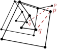
(b)

Figure 15: A schematic drawing of $\operatorname{RNG}_{i}$. (a) The edge $pq\not\in\operatorname{EMST}(S)$ since there is a face-cycle that both $p$ and $q$ lie on. (b) If $p$ and $q$ were in the same connected component of $\operatorname{RNG}_{i}$, but if there were no face-cycle that contains both of them, then $e_{i}$ would cross an edge of $\operatorname{RNG}_{i}$, contradicting the planarity of $\operatorname{RNG}(S)$.

Observation 4.1 tells us that we can identify edges of $\operatorname{EMST}(S)$ if we can determine for each $e_{i}$ the face-cycles in $\operatorname{RNG}_{i}$ that contain the endpoints of $e_{i}$, for $i\in\{1,\dots,m\}$. To accomplish this task, we use the next lemma to traverse the face-cycles.

Lemma 4.2.

Let $i,j\in\{1,\dots,m\}$ and $i>j$. Suppose we are given the length $|e_{i}|$ of $e_{i}\in E_{R}$, a half-edge $\overrightarrow{e_{j}}$ of $e_{j}\in E_{R}$ and the edges incident to the head of $\overrightarrow{e_{j}}$ in $\operatorname{RNG}(S)$ (there are at most six such edges). Let $F$ be the face-cycle of $\operatorname{RNG}_{i}$ that $\overrightarrow{e_{j}}$ lies on. We can find the next half-edge of $\overrightarrow{e_{j}}$ on $F$ in $O(1)$ time using $O(1)$ cells of workspace.

Proof.

Let $\overrightarrow{f_{j}}$ be the next half-edge of $\overrightarrow{e_{j}}$ on $F$. Let $q$ be the head of $\overrightarrow{e_{j}}$. By comparing the length of the edges incident to $q$ in $\operatorname{RNG}(S)$ with $|e_{i}|$, we identify the ones that appear in $\operatorname{RNG}_{i}$, in $O(1)$ time. Then, among them we pick the half-edge $\overrightarrow{f_{j}}$ which has the smallest clockwise angle with $\overrightarrow{e_{j}}$ around $q$ and has $q$ as its tail. This takes $O(1)$ time using $O(1)$ cells of workspace; see Figure 16. ∎

Figure 16: For $i>j$, a schematic drawing of a face-cycle $F$ of $\operatorname{RNG}_{i}$, and $\overrightarrow{e_{j}}$ on $F$ with the head vertex $q$, as well as the other edges of $\operatorname{RNG}_{i}$ incident to $q$. The edge $\overrightarrow{f_{j}}$ which has the smallest clockwise angle with $\overrightarrow{e_{j}}$ is the next edge of $\overrightarrow{e_{j}}$ on $F$.

Lemma 4.3.

Let $i,j\in\{1,\dots,m\}$ and $i\leq j$. Suppose we are given the length $|e_{i}|$ of $e_{i}\in E_{R}$, a half-edge $\overrightarrow{e_{j}}$ of $e_{j}\in E_{R}$ and the edges incident to the head of $\overrightarrow{e_{j}}$ in $\operatorname{RNG}(S)$ (there are at most six such edges). We can find $\text{pre}(\overrightarrow{e_{j}})$ and $\text{suc}(\overrightarrow{e_{j}})$ in $\operatorname{RNG}_{i}$ in $O(1)$ time using $O(1)$ cells of workspace.

Proof.

Let $q$ be the head of $\overrightarrow{e_{j}}$. By comparing the length of the edges incident to $q$ in $\operatorname{RNG}(S)$ with $|e_{i}|$, we identify the incident half-edges of $q$ in $\operatorname{RNG}_{i}$ in $O(1)$ time. Then, among them we pick the half-edge $\text{pre}(\overrightarrow{e_{j}})$ which has $q$ as its head and makes the smallest counterclockwise angle with $\overrightarrow{e_{j}}$ around $w$. Similarly, we pick the half-edge $\text{suc}(\overrightarrow{e_{j}})$ which has $q$ as its tail and makes the smallest clockwise angle with $\overrightarrow{e_{j}}$. This takes $O(1)$ time using $O(1)$ cells of workspace; see Figure 17. ∎

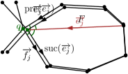
Figure 17: For $i\leq j$, a schematic drawing of $\operatorname{RNG}_{i}$ (in black) and a half-edge $\overrightarrow{e_{j}}$ with head $q$. The half-edge $\text{suc}(\overrightarrow{e_{j}})$ has the smallest clockwise angle with $\overrightarrow{e_{j}}$. The half-edge $\text{pre}(\overrightarrow{e_{j}})$ has the smallest counterclockwise angle with $\overrightarrow{e_{j}}$.

4.2 The Algorithm

From our observations so far, we can derive a simple time-space trade-off for computing $\operatorname{EMST}(S)$. In Theorem 4.4, we simulate Kruskal’s algorithm on $\operatorname{RNG}(S)$. For this, we take batches of $s$ edges of $\operatorname{RNG}(S)$, and we report the edges of $\operatorname{EMST}(S)$ among them. To determine whether an edge $e_{i}$ of $\operatorname{RNG}(S)$ is in $\operatorname{EMST}(S)$, we apply Observation 4.1, i.e., we determine whether the endpoints of $e_{i}$ are on a common face-cycle in the corresponding $\operatorname{RNG}_{i}$.

Theorem 4.4.

Let $S$ be a planar set of $n$ point-sites in general position stored in a read-only array. Let $s\in\{1,\dots,n\}$ be a parameter. We can output all the edges of $\operatorname{EMST}(S)$, in sorted order of their length, in $O\big{(}(n^{3}/s)\log s\big{)}$ time using $O(s)$ cells of workspace.

Proof.

Let $E_{R}=e_{1},\dots,e_{m}$ be the sequence of edges of $\operatorname{RNG}(S)$, sorted by length. In the first iteration, we use Lemma 3.3 to find the batch $e_{1},\dots,e_{s}$ of the first $s$ edges in $E_{R}$ in $O\big{(}(n^{2}/s)\log s\big{)}$ time. For each edge $e_{i}$, $i\in\{1,\dots,s\}$, we consider both its half-edges. Then, we perform $2s$ parallel walks starting from the head vertex of each half-edge $\overrightarrow{e_{i}}$. In the first step of the walks, using Lemma 3.1, we find the incident edges to the head of each half-edge $\overrightarrow{e_{i}}$ (there are at most six such edges). Then, using Lemma 4.3, we identify $\text{pre}(\overrightarrow{e_{i}})$ and $\text{suc}(\overrightarrow{e_{i}})$ in $\operatorname{RNG}_{i}$ (if they exist). By following the successor of each half-edge, we perform one step of the walk for each half-edge of the batch in parallel. Note that the walk that starts from the head of $\overrightarrow{e_{i}}$ takes place in $\operatorname{RNG}_{i}$.

Next, in the second step of the parallel walks, we consider the head vertices of all the $\text{suc}(\overrightarrow{e_{i}})$. First, we use Lemma 3.1 to find the incident edges to the head of each $\text{suc}(\overrightarrow{e_{i}})$ (there are at most six such edges). Then, applying Lemma 4.2, we find the next half-edge of $\text{suc}(\overrightarrow{e_{i}})$, and we advance each half-edge along its face-cycle in $\operatorname{RNG}_{i}$ as one step of the parallel walks. We proceed the parallel walks by finding the next edge on the face-cycles in each step.

A walk that started from the head $q$ of $\overrightarrow{e_{i}}$ continues until it either encounters the tail $p$ of $\overrightarrow{e_{i}}$ or until it arrives at $\text{pre}(\overrightarrow{e_{i}})$. In the former case, we have found a face-cycle that both endpoints of $e_{i}$ lie on and thus, by Observation 4.1, $e_{i}$ is not in $\operatorname{EMST}(S)$; see Figure 18(a). In the latter case, there is no face-cycle in $\operatorname{RNG}_{i}$ that contains both $p$ and $q$. This is because, by definition of $\text{pre}(\overrightarrow{e_{i}})$ and $\text{suc}(\overrightarrow{e_{i}})$, all the incident edges of $q$ in $\operatorname{RNG}_{i}$ lie in the counterclockwise cone between $\text{pre}(\overrightarrow{e_{i}})$ and $\text{suc}(\overrightarrow{e_{i}})$ around $q$. Therefore, by planarity of $\operatorname{RNG}_{i}$, all the other face-cycles that contain $q$ are separated from $p$ by the face-cycle that starts with $\text{suc}(\overrightarrow{e_{i}})$ and ends at $\text{pre}(\overrightarrow{e_{i}})$. Hence, none of those face-cycles encounters $p$ and, by Observation 4.1, $e_{i}$ is an edge of $\operatorname{EMST}(S)$; see Figure 18(b). In this case, we report $e_{i}$, and we also abort the walk that was started from the opposite half-edge of $\overrightarrow{e_{i}}$. This prevents an edge of $\operatorname{EMST}(S)$ to be reported twice.

(a)

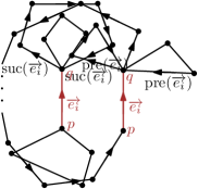
(b)

Figure 18: A schematic drawing of $\operatorname{RNG}_{i}$ and the half-edge $\overrightarrow{e_{i}}$ with head $q$ and tail $p$. (a) The vertices $p$ and $q$ are on the same face-cycle of $\operatorname{RNG}_{i}$ since by traversing the face-cycle starting from $\text{suc}(\overrightarrow{e_{i}})$ we encounter $p$. (b) The vertices $p$ and $q$ are on different face-cycles of $\operatorname{RNG}_{i}$ since by traversing the face-cycle starting from $\text{suc}(\overrightarrow{e_{i}})$ we encounter $\text{pre}(\overrightarrow{e_{i}})$, meaning that we will not reach $p$.

In the next iteration of the algorithm, we again use Lemma 3.3 to find the next batch of $s$ edges in $E_{R}$. Similarly, we perform $2s$ parallel walks for the half-edges in this batch, in order to find the edges that belong to $\operatorname{EMST}(S)$.

Since there are $O(n)$ half-edges in $\operatorname{RNG}(S)$, it takes $O(n)$ steps in each iteration to conclude all the walks, where each step of the walks takes $O(n\log s)$ time. It follows that we can process a single batch of edges in $O(n^{2}\log s)$ time which dominates the time needed for finding a batch of $s$ edges of $\operatorname{RNG}(S)$. We have $O(n/s)$ batches, so the total running time of the algorithm is $O\big{(}(n^{3}/s)\log s\big{)}$. The algorithm uses $O(s)$ cells of workspace for finding and storing a batch of $s$ edges as well as a constant number of cells per edge to perform each walk. ∎

Note that, in this algorithm, it is not essential to process edges of $\operatorname{RNG}(S)$ in sorted order of length. Thus, we can simply apply Lemma 3.1 to produce edges of $\operatorname{RNG}(S)$. However, by using Lemma 3.3 we are able to report edges of $\operatorname{EMST}(S)$ in sorted order of length, although the total running time of the algorithm will not be affected.

5 Improvement via a Compact Representation of RNGs

Theorem 4.4 is clearly not optimal: for the case of linear space $s=n$, we get a running time of $O(n^{2}\log n)$, although we know that it is possible to find $\operatorname{EMST}(S)$ in $O(n\log n)$ time. Can we do better? The bottleneck in Theorem 4.4 is the time needed to perform the walks in the partial relative neighborhood graphs $\operatorname{RNG}_{i}$. In particular, such a walk might take $\Omega(n)$ steps, leading to a running time of $\Omega(n^{2}\log s)$ for processing a single batch of $s$ edges. To avoid this, we will maintain a compressed representation of the partial relative neighborhood graphs that allows us to reduce the number of steps in each walk to $O(n/s)$.

5.1 The $s$-net Structure

Let $i\in\{1,\dots,m\}$. An $s$-net $N$ for $\operatorname{RNG}_{i}$ is a collection of half-edges, called net-edges, in $\operatorname{RNG}_{i}$ that has the following two properties: (i) Each face-cycle in $\operatorname{RNG}_{i}$ with at least $\lfloor n/s\rfloor+1$ half-edges contains at least one net-edge. (ii) For any net-edge $\overrightarrow{e}\in N$, let $F$ be the face-cycle of $\operatorname{RNG}_{i}$ that contains $\overrightarrow{e}$. Then on $F$, between the head of $\overrightarrow{e}$ and the tail of the next net-edge, there are at least $\lfloor n/s\rfloor$ and at most $2\lfloor n/s\rfloor$ other half-edges. Note that the next net-edge on $F$ after $\overrightarrow{e}$ could possibly be $\overrightarrow{e}$ itself. In particular, this implies that face-cycles with less than $\lfloor n/s\rfloor$ edges contain no net-edges; see Figure 19.

(a)

(b)

(c)

Figure 19: A schematic drawing of an $s$-net for $\operatorname{RNG}_{i}$. (a) A small face-cycle with no net-edges. (b) a face-cycle with more than $\lfloor n/s\rfloor$ and less than $2\lfloor n/s\rfloor$ half-edges which contains one net-edge. (c) A big face-cycle with four net-edges.

We note two important observations about $s$-nets.

Observation 5.1.

Let $i\in\{1,\dots,m\}$, and let $N$ be an $s$-net for $\operatorname{RNG}_{i}$. Then,

1. $N$ has $O(s)$ half-edges; and

2. let $\overrightarrow{f}$ be a half-edge of $\operatorname{RNG}_{i}$, and let $F$ be the face-cycle that contains it. Then, it takes at most $2\lfloor n/s\rfloor$ steps along $F$ from the head of $\overrightarrow{f}$ until we encounter the tail of either a net-edge or $\overrightarrow{f}$ itself.

Proof.

Property (ii) of the definition of an $s$-net implies that only face-cycles of $\operatorname{RNG}_{i}$ with at least $\lfloor n/s\rfloor+1$ half-edges contain net-edges. Furthermore, on these face-cycles, we can uniquely charge $\Theta(n/s)$ half-edges to each net-edge, again by property (ii). Since the face-cycles of $\operatorname{RNG}_{i}$ have $O(n)$ half-edges in total, we obtain the first observation which says $|N|=O(s)$.

For the second observation, we first note that if $F$ contains less than $2\lfloor n/s\rfloor$ half-edges, the claim holds trivially. Otherwise, by property (i), $F$ contains at least one net-edge. From property (ii) it follows that there are at most $2\lfloor n/s\rfloor$ half-edges between every two consecutive net-edges on $F$. Thus, in a walk on $F$ starting from $\overrightarrow{f}$, we reach a net-edge in at most $2\lfloor n/s\rfloor$ steps. ∎

Due to statement (N1) of Observation 5.1, an $s$-net can be stored in $O(s)$ cells of workspace. This makes the concept of $s$-net useful in our algorithm with a workspace of $O(s)$ cells. Therefore, we can exploit the $s$-net in order to speed up the processing of a single batch. The next lemma shows how this is done.

Lemma 5.2.

Let $i\in\{1,\dots,m\}$. Suppose we are given $E_{i,s}=e_{i},\dots,e_{i+s-1}$, a batch of $s$ edges in $E_{R}$. Furthermore, we have an $s$-net $N$ for $\operatorname{RNG}_{i}$ in our workspace. Then, we can determine which edges from $E_{i,s}$ belong to $\operatorname{EMST}(S)$ in $O\big{(}(n^{2}/s)\log s\big{)}$ time using $O(s)$ cells of workspace.

Proof.

Let $H$ be a set of half-edges defined as follows: the set $H$ is the union of all net-edges from $N$, and, for each batch-edge $e_{j}\in E_{i,s}$, the successors of the two half-edges of $e_{j}$ in $\operatorname{RNG}_{i}$; see Figure 20.

Figure 20: A schematic drawing of $\operatorname{RNG}_{i}$ with a batch of edges in $E_{R}$ (dashed red segments). The directed segments represents the half-edges in $H$. The net-edges are in green and the successors of the batch edges are in black.

By definition, we have $|H|=O(s)$, and thus it takes $O(n\log s)$ time to compute $H$. This is done by using Lemma 3.1 to find the incident edges of the head of each $e_{j}$ and Lemma 4.3 to identify the successors of each $e_{j}$.

Now starting from the half-edges in $H$, we perform parallel walks through the face-cycles of $\operatorname{RNG}_{i}$, one walk per half-edge. Each such walk proceeds until it encounters the tail of a half-edge in $H$ (including the starting half-edge itself). In each step of these walks, we use Lemma 3.1 and Lemma 4.2 to find the next half-edges on the face-cycles in $O(n\log s)$ time, and then we check whether these new half-edges belong to $H$ in $O(s\log s)$ time. Because $H$ contains the net-edges of $N$, by statement (N2) of Observation 5.1, each walk finishes after $O(n/s)$ steps, and thus, the total time for this procedure is $O\big{(}(n^{2}/s)\log s\big{)}$.

Next, we build an auxiliary undirected (multi-)graph $G$ as follows: the vertices of $G$ are the endpoints of the half-edges in $H$ and the endpoints of the half-edges of $E_{i,s}$. Furthermore, $G$ contains undirected edges for all the half-edges in $H$ and additional compressed edges, that represent the outcomes of the walks: if a walk started from the head $q$ of a half-edge in $H$ and ended at the tail $p$ of a half-edge in $H$, we add an edge from $q$ to $p$ in $G$, and we label it with the number of steps that were needed for the walk, i.e., the number of half-edges between $q$ and $p$ on that face-cycle. Thus, $G$ contains $H$-edges, and compressed edges; see Figure 21. Clearly, after all the walks have been terminated, we can construct $G$ in $O(s)$ time, using $O(s)$ cells of workspace.

Figure 21: The auxiliary graph $G$ is shown. The edge set of $G$ contains the net-edges (in green), the successors of batch-edges (in black), and the compressed edges (beige paths).

The auxiliary graph $G$ is actually a representation of the face-cycles in $\operatorname{RNG}_{i}$. Thus, by adding the batch-edges of $E_{i,s}$ one by one into $G$, we can represent the next partial relative neighborhood graphs, up to $\operatorname{RNG}_{i+s}$. Hence, we can use $G$ to identify which of the batch-edges of $E_{i,s}$ belong to $\operatorname{EMST}(S)$. This is done by applying Kruskal’s algorithm on $G$ as follows: we determine the connected components of $G$ in $O(s)$ time using depth-first search. Then, we insert the batch-edges into $G$, one after another, in sorted order. As we do this, we keep track of how the connected components of $G$ change, using a union-find data structure [15]. Whenever a new batch-edge connects two distinct connected components of $G$, we output it as an edge of $\operatorname{EMST}(S)$. Otherwise, we do nothing; see Figure 22. Note that even though one component of $\operatorname{RNG}_{i}$ might be represented by several components in $G$,, the algorithm is still correct because of Observation 4.1.

This execution of Kruskal’s algorithm and updating the structure of connected components of $G$ takes $O(s\log s)$ time, which is dominated by the running time of $O\big{(}(n^{2}/s)\log s\big{)}$ to perform the parallel walks. The space requirement for constructing and storing the set $H$ and the graph $G$ as well as the updated versions of $G$ is a total of $O(s)$ cells of workspace. ∎

Figure 22: The batch-edges of $E_{i,s}$ (in red) have been added to the auxiliary graph $G$.

5.2 Maintaining the $s$-net

Now that we have described how to use an $s$-net for $\operatorname{RNG}_{i}$ in order to process the edges $e_{i},\dots,e_{i+s}$ of $E_{R}$, we need to explain how to maintain the $s$-net during the algorithm, i.e., how to construct an $s$-net for $\operatorname{RNG}_{i+s}$ after processing the edges $e_{i},\dots,e_{i+s}$. The algorithm in the following lemma computes an $s$-net for $\operatorname{RNG}_{i+s}$, provided that we have an $s$-net for $\operatorname{RNG}_{i}$ as well as the graph $G$ as it is constructed in the proof of Lemma 5.2, for each $i\in\{1,\dots,m\}$.

Lemma 5.3.

Let $i\in\{1,\dots,m\}$, and suppose we have the graph $G$ derived from $\operatorname{RNG}_{i}$ as above, such that all batch-edges have been inserted into $G$. Then, we can compute an $s$-net $N$ for $\operatorname{RNG}_{i+s}$ in time $O\big{(}(n^{2}/s)\log s\big{)}$, using $O(s)$ cells of workspace.

Proof.

By construction, all big face-cycles of $\operatorname{RNG}_{i+s}$, i.e., those face-cycles with at least $\lfloor n/s\rfloor+1$ half-edges, appear as faces in $G$. Thus, by walking along all faces in $G$, and taking into account the labels of the compressed edges, we can determine these big face-cycles in $O(s)$ time. The big face-cycles are represented through sequences of $H$-edges, compressed edges, and batch-edges. For each such sequence, we determine the positions of the half-edges for the new $s$-net $N$, by spreading the half-edges equally at minimum distance $\lfloor n/s\rfloor$ and maximum distance $2\lfloor n/s\rfloor$ along the sequence, again taking the labels of the compressed edges into account. Since the compressed edges have length $O(n/s)$, for each of them, we create at most $O(1)$ new net-edges. Now that we have determined the positions of the new net-edges on the face-cycles of $\operatorname{RNG}_{i+s}$, we perform $O(s)$ parallel walks in $\operatorname{RNG}_{i+s}$ to actually find them. Using Lemma 3.1 and Lemma 4.2, this takes $O\big{(}(n^{2}/s)\log s\big{)}$ time; see Figure 23. ∎

(a)

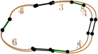
(b)

Figure 23: (a) A schematic drawing of a face-cycle in $G$ and (b) distributing the new net-edges (in green) on this face-cycle with almost equal distances.

We now have all the ingredients for our main result that provides a smooth trade-off between the cubic-time algorithm in constant workspace and the classic $O(n\log n)$-time algorithm with $O(n)$ cells of workspace. The following theorem presents this algorithm.

Theorem 5.4.

Let $S$ be a planar set of $n$ point-sites in general position stored in a read-only array. Let $s\in\{1,\dots,n\}$ be a parameter. We can report all the edges of $\operatorname{EMST}(S)$, in sorted order of length, in $O\big{(}(n^{3}/s^{2})\log s\big{)}$ time using $O(s)$ cells of workspace.

Proof.

This follows immediately from our lemmas: applying Lemma 3.3, we produce a batch of $s$ edges of $\operatorname{RNG}(S)$ in sorted order of length. Then, among them, we report the edges of $\operatorname{EMST}(S)$, using Lemma 3.3. Finally, we maintain the $s$-net structure to be used for the next batch of $s$ edges of $\operatorname{RNG}(S)$, by Lemma 5.3. All these steps are done in $O\big{(}(n^{2}/s)\log s\big{)}$ time using $O(s)$ cells of workspace. Since $\operatorname{RNG}(S)$ has $O(n)$ edges, we need to process $O(n/s)$ batches of edges of $\operatorname{RNG}(S)$, leading to an algorithm with total running time of $O\big{(}(n^{3}/s^{2})\log s\big{)}$, and total workspace usage of $O(s)$ cells. ∎

6 Conclusion

For our algorithm, it suffices to update the $s$-net every time that a new batch is considered. It is, however, possible to maintain the $s$-net and the auxiliary graph $G$ through insertions of single edges, with the same bound as in Lemma 5.3. This allows us to handle graphs constructed incrementally and to maintain their compact representation using $O(s)$ workspace cells. We believe this is of independent interest and can be used by other algorithms for planar graphs in the limited-workspace model.

Also, it remains an intriguing question whether the EMST can be computed in $o(n^{3})$ time in the constant-workspace model. Intuitively, it seems hard to improve the $O(n^{2})$-time algorithm for checking whether an individual edge belongs to the EMST, and maybe it will be possible to obtain a formal lower bound for this subproblem. However, even such a lower bound would not rule out other possible approaches towards a faster EMST-algorithm.

Acknowledgments.

This work was initiated at the Fields Workshop on Discrete and Computational Geometry, held 07.31.–08.04.2017, at Carleton university. The authors would like to thank them and all the participants of the workshop for inspiring discussions and for providing a great research atmosphere.

References

- [1] H.-K. Ahn, N. Baraldo, E. Oh, and F. Silvestri. A time-space trade-off for triangulations of points in the plane. In Proc. 23rd Internat. Comput. and Combinat. Conf. (COCOON), pages 3–12, 2017.
- [2] B. Aronov, M. Korman, S. Pratt, A. van Renssen, and M. Roeloffzen. Time-space trade-offs for triangulating a simple polygon. In Proc. 15th Scand. Symp. Work. Alg. Theory (SWAT), pages 30:1–30:12, 2016.
- [3] S. Arora and B. Barak. Computational Complexity: A Modern Approach. Cambridge University Press, Cambridge, UK, 2009.
- [4] T. Asano and D. G. Kirkpatrick. Time-space tradeoffs for all-nearest-larger-neighbors problems. In Proc. 13th Alg. and Data Struct. Symp. (WADS), pages 61–72, 2013.
- [5] T. Asano, W. Mulzer, G. Rote, and Y. Wang. Constant-work-space algorithms for geometric problems. J. of Computational Geometry, 2(1):46–68, 2011.
- [6] T. Asano, W. Mulzer, and Y. Wang. Constant-work-space algorithms for shortest paths in trees and simple polygons. J. Graph. Alg. Appl., 15(5):569–586, 2011.
- [7] Y. Bahoo, B. Banyassady, P. Bose, S. Durocher, and W. Mulzer. A time-space trade-off for computing the -visibility region of a point in a polygon. Theoret. Comput. Sci., 789:13–21, 2019.
- [8] B. Banyassady, M. Korman, and W. Mulzer. Computational geometry column 67. ACM SIGACT News, 49(2):77–94, 2018.
- [9] B. Banyassady, M. Korman, W. Mulzer, A. van Renssen, M. Roeloffzen, P. Seiferth, and Y. Stein. Improved time-space trade-offs for computing Voronoi diagrams. J. of Computational Geometry, 7(2):19–45, 2018.
- [10] L. Barba, M. Korman, S. Langerman, K. Sadakane, and R. I. Silveira. Space-time trade-offs for stack-based algorithms. Algorithmica, 72(4):1097–1129, 2015.
- [11] L. Barba, M. Korman, S. Langerman, and R. I. Silveira. Computing a visibility polygon using few variables. Comput. Geom. Theory Appl., 47(9):918–926, 2014.
- [12] M. de Berg, O. Cheong, M. van Kreveld, and M. Overmars. Computational Geometry: Algorithms and Applications. Springer-Verlag, Berlin, third edition, 2008.
- [13] T. M. Chan and E. Y. Chen. Multi-pass geometric algorithms. Discrete Comput. Geom., 37(1):79–102, 2007.
- [14] T. M. Chan, J. I. Munro, and V. Raman. Selection and sorting in the “restore” model. In Proc. 25th Annual ACM-SIAM Symp. Disc. Alg. (SODA), pages 995–1004, 2014.
- [15] T. H. Cormen, C. E. Leiserson, R. L. Rivest, and C. Stein. Introduction to Algorithms. MIT Press, Cambridge, MA, USA, third edition, 2009.
- [16] O. Darwish and A. Elmasry. Optimal time-space tradeoff for the 2D convex-hull problem. In Proc. 22nd Annual European Symp. Alg. (ESA), pages 284–295, 2014.
- [17] A. Elmasry and F. Kammer. Space-efficient plane-sweep algorithms. In Proc. 27th Annu. Internat. Sympos. Algorithms Comput. (ISAAC), pages 30:1–30:13, 2016.
- [18] S. Har-Peled. Shortest path in a polygon using sublinear space. J. of Computational Geometry, 7(2):19–45, 2016.
- [19] J. W. Jaromczyk and G. T. Toussaint. Relative neighborhood graphs and their relatives. Proceedings of the IEEE, 80:1502–1517, 1992.
- [20] M. Korman, W. Mulzer, A. van Renssen, M. Roeloffzen, P. Seiferth, and Y. Stein. Time-space trade-offs for triangulations and Voronoi diagrams. Comput. Geom. Theory Appl., 73:35–45, 2018.
- [21] J. S. B. Mitchell and W. Mulzer. Proximity algorithms. In J. E. Goodman, J. O’Rourke, and C. D. Tóth, editors, Handbook of Discrete and Computational Geometry, pages 849–874. CRC Press, third edition, 2017.
- [22] J. I. Munro and M. S. Paterson. Selection and sorting with limited storage. Theoret. Comput. Sci., 12(3):315–323, 1980.
- [23] J. I. Munro and V. Raman. Selection from read-only memory and sorting with minimum data movement. Theoret. Comput. Sci., 165(2):311–323, 1996.
- [24] J. Pagter and T. Rauhe. Optimal time-space trade-offs for sorting. In Proc. 39th IEEE Annual Symp. Found. Comp. Sci. (FOCS), pages 264–268, 1998.
- [25] F. P. Preparata and M. I. Shamos. Computational geometry. An introduction. Springer-Verlag, New York, 1985.
- [26] O. Reingold. Undirected connectivity in log-space. J. ACM, 55(4):17:1–17:24, 2008.
- [27] G. T. Toussaint. The relative neighbourhood graph of a finite planar set. Pattern Recognition, 12(4):261–268, 1980.