Abstract

The special feature of the observations is the usage of the TESIS EUV telescope. The instrument could image the solar corona in the Fe 171 Å line up to a distance of 2 $R_{\odot}$ from the center of the Sun. This allows us to trace the CME up to the LASCO/C2 field of view without losing the CME from sight.

1 Introduction

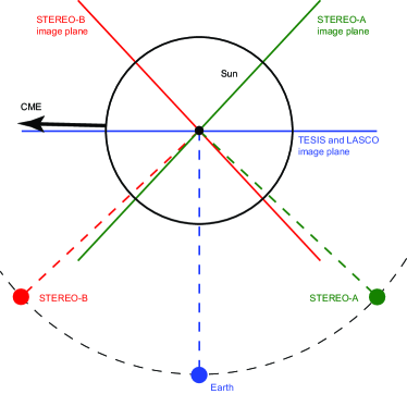
Figure 1:

2 Experimental Data

Table 1: Characteristics of the used instruments.

Satellite	Instrument	Wavelength	Resolution	Field of View	Cadence
CORONAS-PHOTON	TESIS EUV telescope	171 Å	3.4′′	$\leq 2$ $R_{\odot}$	30–60 min
		304 Å	1.7′′	$\leq 2$ $R_{\odot}$	4 min
	Mg XII spectroheliograph	8.42 Å	4.0′′	$\leq 1.6$ $R_{\odot}$	90 min
	SphinX	1–15 keV	—	—	1 min
SOHO	EIT	304 Å	5.3′′	$\leq 1.6$ $R_{\odot}$	12 min
	LASCO/C2	white light	11.4′′	2–6 $R_{\odot}$	20 min
	LASCO/C3	white light	56.0′′	4–30 $R_{\odot}$	30 min
STEREO	EUVI	171 Å	1.6′′	$\leq 1.7$ $R_{\odot}$	2.5 min
		195 Å	1.6′′	$\leq 1.7$ $R_{\odot}$	10 min
		284 Å	1.6′′	$\leq 1.7$ $R_{\odot}$	20 min
		304 Å	1.6′′	$\leq 1.7$ $R_{\odot}$	10 min
	COR1	white light	7.0′′	1.5–4 $R_{\odot}$	5–10 min
	COR2	white light	14.7′′	2.5–15 $R_{\odot}$	15 min

In this study, we the data of the TESIS EUV telescopes and the Mg XII spectroheliograph (Kuzin et al., 2011), the SphinX spectrophotometer (Gburek et al., 2011), the LASCO coronagraphs (Brueckner et al., 1995), and the data of the STEREO satellites (Howard et al., 2008).

TESIS is an instrument assembly that observed the solar corona in the soft X-ray and EUV. It worked on board the CORONAS-PHOTON satellite (Kotov, 2011). The TESIS EUV telescope imaged solar corona in the Fe 171 Å and He 304 Å lines. The special feature of the TESIS EUV telescope was its ability to image corona up to a distance of 2 $R_{\odot}$ from the Sun’s center (for details, see Reva et al., 2014). We use TESIS data to observe coronal magnetic structure and prominence evolution at high altitudes.

The Mg XII spectroheliograph was a part of the TESIS assembly. The instrument built monochromatic images of the solar corona in the Mg XII 8.42 Å line. This line emits at temperatures higher than 4 MK, and the Mg XII images contain only the signal from the hot plasma without any low temperature background. In 2009, the Sun was in the minimum of its activity cycle, and the spectroheligraph Mg XII registered sub-A class flare-like events (Kirichenko & Bogachev, 2017a, b). We use the spectroheliograph Mg XII to study the X-ray emission associated with the analyzed CME.

SphinX is a spectrophotometer that worked on board the CORONAS-PHOTON satellite. SphinX registered solar spectra in the 1–15 keV energy range. In 2009, the solar cycle was in deep minimum, and the GOES flux usually was below the sensitivity threshold. SphinX is more sensitive than GOES, and we use it to see the variation of the X-ray flux.

LASCO is a set of white-light coronagraphs that observe solar corona from 1.1 $R_{\odot}$ up to 30 $R_{\odot}$ (C1, 1.1–3 $R_{\odot}$; C2, 2–6 $R_{\odot}$; C3, 4–30 $R_{\odot}$). In 1998, LASCO C1 stopped working, and today LASCO can only image corona above 2 $R_{\odot}$. We use LASCO data to study the CME above 2 $R_{\odot}$.

STEREO is a set of two satellites: STEREO-A, which moves ahead of the Earth, and STEREO-B, which moves behind the Earth. During the period of our observations, STEREO satellites were separated from the Earth by 47^∘ (see Figure 1). STEREO satellites carry EUVI telescopes that image the solar corona in the 171, 195, 284, and 304 Å lines. We use the STEREO-B EUVI data to determine 3D orientation of the erupting prominence and observe the solar surface that is not seen from the Earth point of view.

Moreover, STEREO satellites carry white-light coronagraphs: COR1, which images corona at distances 1.3–4 $R_{\odot}$, and COR2, 2–15 $R_{\odot}$. We use the COR1 and COR2 data from both satellites to enhance the measurements of the CME kinematics.

3 Results

3.1 Outline of the Observations

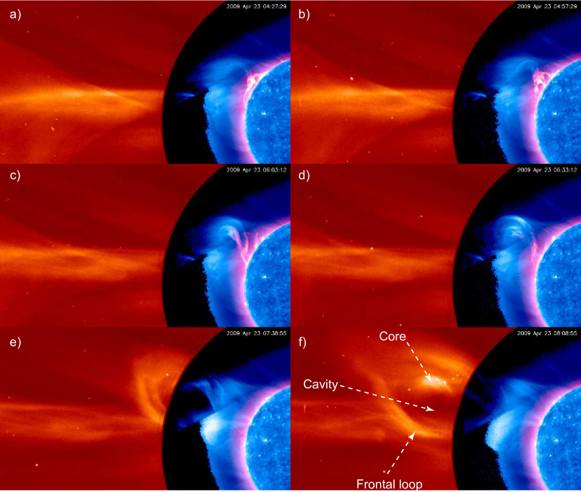
Figure 2: Blue: TESIS Fe 171 Å images; purple: TESIS He 304 Å images; red: LASCO/C2 images. An animation is available for this figure.

the prominence tore apart and drained down, while the fluxrope continued to erupt . In the LASCO/C2 images, the fluxrope corresponded to the CME core. By the time the fluxrope had reached the LASCO/C2 field of view, the prominence had already drained down to the solar surface.

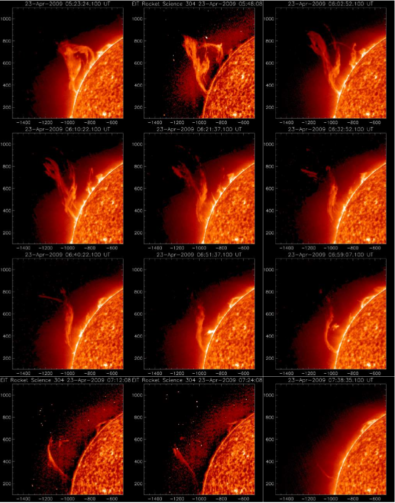
Figure 3: Draining of the prominence. These are TESIS and EIT He 304 Å images. Coordinates are measured in arcseconds. An animation is available for this figure.

. During the first acceleration phase, we observed signatures of flare reconnection: an increase in the X-ray flux and a two-ribbon flare. There were no signatures of reconnection during the second acceleration phase.

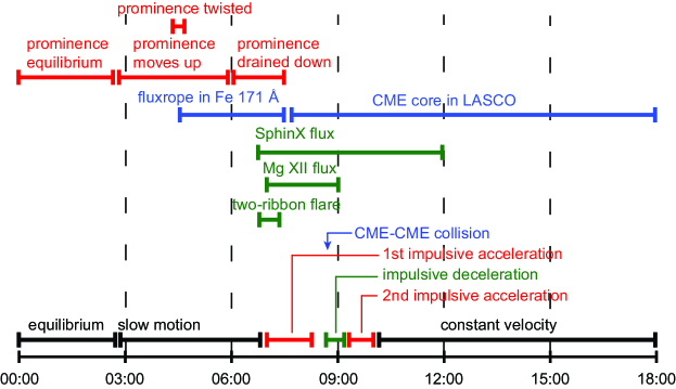
Figure 4: Summary of the observations.

Table 2: Summary of the observations.

Time, UT	Description
$\approx$ 02:51	prominence started to move up
$\approx$ 04:27	CME core appeared in the TESIS Fe 171 Å images
$\approx$ 06:02	prominence started to drain
$\approx$ 07:38	prominence drained down
$\approx$ 07:38	the core passed to the LASCO/C2 field of view
	the first impulsive acceleration phase
$\approx$ 06:45–12:00	the SphinX X-ray flux
$\approx$ 07:00–09:00	the Mg XII spectroheliograph X-ray flux
$\approx$ 06:46–07:20	motion of the flare ribbons
	the second impulsive acceleration phase

3.2 Sequence of Events

In the STEREO-B EUVI images, the prominence looked like a filament was inclined by 25^∘ to the meridian and was close to the TESIS limb (see Figure 5). the prominence eruption occurred almost entirely in the TESIS image plane (see Figure 1).

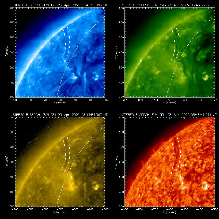
Figure 5: Erupting prominence (filament) in the STEREO EUVI-B images. Dashed lines mark the filament; solid line designates the TESIS limb.

The prominence started to lift at 02:51 UT on . At 04:28 UT, in the Fe 171 Å images, a fluxrope formed. the prominence twisted at $\approx$ 04:35 UT (see Figure 6).

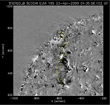
Figure 6: Twisting of the prominence. This is a running difference image the EUVI-B 195 Å channel. dashed lines indicate the prominence.

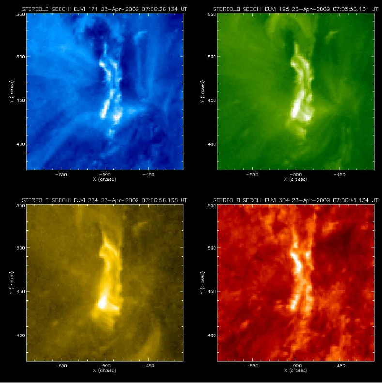
Figure 7: Two-ribbon flare observed by STEREO-B EUVI.

We observed in the Mg XII spectroheliograph images (see Figure 8). This source corresponds to the flare arcade below the CME. It was the only X-ray source on the Sun.

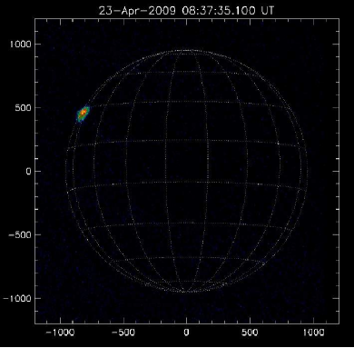
Figure 8: Coordinates are measured in arc seconds.

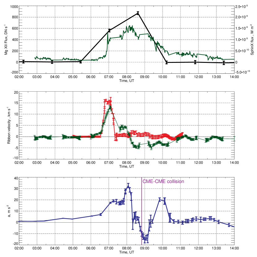
Figure 9: Black: ; green top: the SphinX flux convolved with the response function of the GOES 1–8 Å channel; green : the SphinX flux; red: the velocity of the flare ; blue: .

During the period of the observations, the GOES X-ray flux sensitivity threshold. , the SphinX registered an increase of the X-ray flux. Since the Mg XII spectroheliograph observed only one X-ray source, the increase of the SphinX flux comes entirely from the flare arcade.

We convolved the SphinX spectrum with the response function of the GOES 1–8 Å channel and obtained a synthetic GOES flux (see Figure 9, top). The studied flare arcade A0.15 GOES class.

The prominence was located in the lowest parts of the magnetic structure visible in the Fe 171 Å images. While erupting, the magnetic structure dragged the prominence up. At the altitude of 220 Mm above the solar surface, the prominence tore apart and started to drain while the fluxrope continued to erupt .

The gap between the LASCO/C2 and TESIS fields of view is small. This allows us to track the CME without losing it from sight. In the LASCO/C2 images, the CME had a three-part structure: core, cavity, and frontal loop (see Figure 2f). The CME core in the LASCO images corresponds to the fluxrope center observed in the Fe 171 Å images. When the CME core the TESIS field of view, the prominence had already drained down.

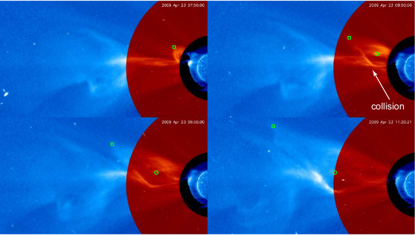
Figure 10: CME-CME collision. Outer blue: LASCO/C3 images, red: LASCO/C2 images, inner blue: TESIS Fe 171 Å images. Circle marks the CME core. Rectangle marks part of the frontal loop. Marked parts were used to measure CME kinematics. An animation is available for this figure.

3.3 Analysis

3.3.1 CME Kinematics

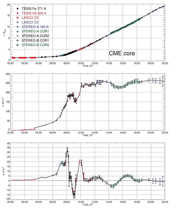
Figure 11: . $r(t)$ is the distance from the CME core to the center, $v(t)$ is the CME core radial velocity, $a(t)$ is the CME core radial acceleration.

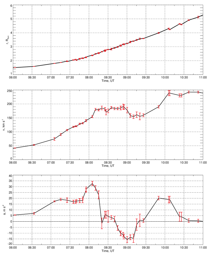
Figure 12: . $r(t)$ is the distance from the CME core to the center, $v(t)$ is the CME core radial velocity, $a(t)$ is the CME core radial acceleration.

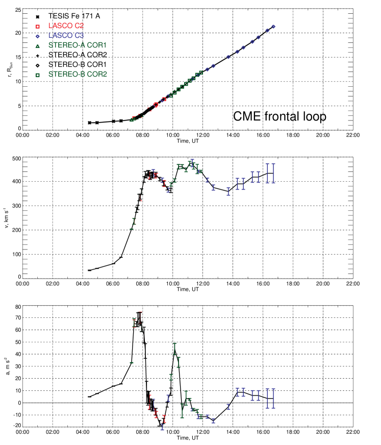
Figure 13: $r(t)$ is the distance from the CME frontal loop to the center, $v(t)$ is the CME frontal loop radial velocity, $a(t)$ is the CME frontal loop radial acceleration.

We measured the coordinates of in the TESIS Fe 171 Å and He 304 Å, LASCO C2 and C3 images a simple point and click method. times to make this method less subjective, and estimate error bars.

The studied CME was also observed by the STEREO-A (EUVI 195 Å, COR1 and COR2) and STEREO-B (COR1 and COR2). We measured the CME core trajectories in these images using the same method.

TESIS/LASCO, STEREO-A, and STEREO-B observed the event from different view-points. The instruments responded differently to temperature and density. The positions of the CME core determined subjectively. Due to these factors, if we put the values $r(t)$ measured by different instruments on the same plot, the values will slightly differ from each other (even after the correction of the projection effects).

To correct the discrepancy, we adopted the procedure from Reva et al. (2016b). First, we scaled the values obtained from STEREO-A and STEREO-B using the separation angles of the satellites. After this procedure, the STEREO points slightly deviated from the TESIS/LASCO points.

We assumed that the CME expanded uniformly, and scaled each of the STEREO channels to fit the TESIS/LASCO plot (see Table 3). As a result, we obtained a composite kinematics plot consisting of 139 points

Table 3: Kinematics scaling multiplier.

Channel	Core	Frontal loop
STEREO-A EUVI 195 Å	0.93	—
STEREO-A COR1	0.83	0.82
STEREO-A COR2	1.00	0.80
STEREO-B COR1	0.82	0.90
STEREO-B COR2	0.97	0.84

We numerically differentiate $r(t)$ and obtain radial velocity $v(t)$ and radial acceleration $a(t)$.

3.3.2 Flare Ribbons Motion

During the eruption, two-ribbon flare occurred below the CME (see Figure 7). The speed of the ribbon separation reflects the reconnection rate in the current sheet (Qiu et al., 2004). The faster the ribbons move, the higher the reconnection rate.

We measured the distance between the ribbons in the EUVI-B images using a point-and-click procedure. The main source of errors in this method is the subjectivity. To eliminate subjectivity and estimate error bars, we repeated the procedure multiple times. we corrected the result for the projection effect.

Before 06:46 UT, the two-ribbon flare was not seen in the EUVI-B images. We added “zero points” to the plot: zero values at times when the EUVI-B took images, but the two-ribbon flare was absent.

From 06:45 UT to 07:15 UT, the ribbons moved with a roughly constant speed of 15 km s^-1 (see Figure 14). After 07:15 UT, the distance between the footpoints was constant within error margins.

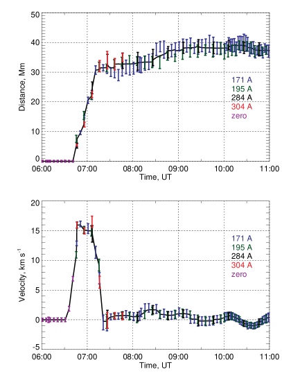
Figure 14: Blue: EUVI-B 171 Å channel; green: EUVI-B 195 Å channel; black: EUVI-B 284 Å channel; red: EUVI-B 304 Å channel; purple: “zero points” (171 Å images without flare ribbons).

3.3.3 X-ray Flux

The derivative of the soft X-ray flux reflects the reconnection rate (Neupert, 1968).

The derivative of the SphinX flux and the flare velocity have peaks that correlate with the first impulsive CME acceleration phase (see Figure 9, bottom). During the second phase, there were no .

4 Discussion

4.1 Initiation of the CME

In , a CME erupts due to the draining of mass from the CME pre-erupting structure (Fan & Low, 2003). If, for some reason, part of the CME mass drains out, , and the CME will erupt.

, the CME loses mass before an eruption. In our observations, the CME lost the mass the eruption.

4.2 Two Impulsive Acceleration Phases

The studied CME had two impulsive acceleration phases.

$$v_{A}\approx\frac{L}{\tau}\approx 250\ \text{kms^{-1},}$$ (1)

4.3 CME Core and a Prominence

In white-light coronagraph images, approximately 30% of CMEs have a three-part structure: bright core, dark cavity, and bright frontal loop (Illing & Hundhausen, 1985; Webb & Hundhausen, 1987). It is possible that more CMEs have a three-part structure, but we do not see it .

Illing & Athay (1986) compared white-light and $H_{\alpha}$ images of the SMM coronagraphs (Hundhausen, 1999), and showed that several CMEs contained cold prominence plasma inside their cores. In white-light coronagraphs images, the CME core often looks like a prominence ( long linear twisted structure; Plunkett et al., 2000). Since the core resembles the prominence and some CME cores contained prominence plasma, the core is usually interpreted as erupting prominence (House et al., 1981; Webb & Howard, 2012; Parenti, 2014).

However, a CME core could have a wide range of temperatures: cool (0.03–0.3 MK; Akmal et al., 2001; Ciaravella et al., 1997, 1999, 2000), warm ($\approx$1 MK; Ciaravella et al., 2003; Landi et al., 2010; Reva et al., 2016a), or hot (5–10 MK; Reeves & Golub, 2011; Song et al., 2014; Nindos et al., 2015). The warm and hot plasma inside the CME cores could be interpreted in two ways: the prominence is heated during the eruption (Filippov & Koutchmy, 2002) or the CME core is not a prominence. As we see, the relationship between core and the prominence is unclear.

In this work, we studied a CME with a three-part structure in the LASCO images. Its core corresponded to the fluxrope, observed in the Fe 171 Å images. However, TESIS He 304 Å images showed that the prominence drained down, before the CME reached the LASCO field of view.

5 Conclusion

During the first phase,

The studied event shows that CMEs are complex phenomena that cannot be explained only one acceleration mechanism. We should seek a combination of different mechanisms that accelerate CMEs at different stages of their evolution.

References

- Akmal et al. (2001) Akmal, A., Raymond, J. C., Vourlidas, A., et al. 2001, ApJ, 553, 922
- Alissandrakis et al. (2013) Alissandrakis, C. E., Kochanov, A. A., Patsourakos, S., et al. 2013, PASJ, 65, 8
- Antiochos et al. (1999) Antiochos, S. K., DeVore, C. R., & Klimchuk, J. A. 1999, ApJ, 510, 485
- Aulanier (2014) Aulanier, G. 2014, in IAU Symposium, Vol. 300, Nature of Prominences and their Role in Space Weather, ed. B. Schmieder, J.-M. Malherbe, & S. T. Wu, 184–196
- Bein et al. (2012) Bein, B. M., Berkebile-Stoiser, S., Veronig, A. M., Temmer, M., & Vršnak, B. 2012, ApJ, 755, 44
- Bemporad et al. (2007) Bemporad, A., Raymond, J., Poletto, G., & Romoli, M. 2007, ApJ, 655, 576
- Brueckner et al. (1995) Brueckner, G. E., Howard, R. A., Koomen, M. J., et al. 1995, Sol. Phys., 162, 357
- Byrne et al. (2014) Byrne, J. P., Morgan, H., Seaton, D. B., Bain, H. M., & Habbal, S. R. 2014, Sol. Phys., 289, 4545
- Carmichael (1964) Carmichael, H. 1964, NASA Special Publication, 50, 451
- Chen (2011) Chen, P. F. 2011, Living Reviews in Solar Physics, 8, doi:10.12942/lrsp-2011-1
- Ciaravella et al. (2003) Ciaravella, A., Raymond, J. C., van Ballegooijen, A., et al. 2003, ApJ, 597, 1118
- Ciaravella et al. (1997) Ciaravella, A., Raymond, J. C., Fineschi, S., et al. 1997, ApJ, 491, L59
- Ciaravella et al. (1999) Ciaravella, A., Raymond, J. C., Strachan, L., et al. 1999, ApJ, 510, 1053
- Ciaravella et al. (2000) Ciaravella, A., Raymond, J. C., Thompson, B. J., et al. 2000, ApJ, 529, 575
- Delaboudinière et al. (1995) Delaboudinière, J., Artzner, G. E., Brunaud, J., et al. 1995, Sol. Phys., 162, 291
- D’Huys et al. (2017) D’Huys, E., Seaton, D. B., De Groof, A., Berghmans, D., & Poedts, S. 2017, Journal of Space Weather and Space Climate, 7, A7
- Fan & Low (2003) Fan, Y., & Low, B. C. 2003, in Astronomical Society of the Pacific Conference Series, Vol. 286, Current Theoretical Models and Future High Resolution Solar Observations: Preparing for ATST, ed. A. A. Pevtsov & H. Uitenbroek, 347
- Filippov & Koutchmy (2002) Filippov, B., & Koutchmy, S. 2002, Sol. Phys., 208, 283
- Gburek et al. (2011) Gburek, S., Sylwester, J., Kowalinski, M., et al. 2011, Solar System Research, 45, 189
- Gosain et al. (2016) Gosain, S., Filippov, B., Ajor Maurya, R., & Chandra, R. 2016, ApJ, 821, 85
- Hirayama (1974) Hirayama, T. 1974, Sol. Phys., 34, 323
- Hood & Priest (1981) Hood, A. W., & Priest, E. R. 1981, Geophysical and Astrophysical Fluid Dynamics, 17, 297
- House et al. (1981) House, L. L., Wagner, W. J., Hildner, E., Sawyer, C., & Schmidt, H. U. 1981, ApJ, 244, L117
- Howard et al. (2008) Howard, R. A., Moses, J. D., Vourlidas, A., et al. 2008, Space Sci. Rev., 136, 67
- Hundhausen (1999) Hundhausen, A. 1999, in The many faces of the sun: a summary of the results from NASA’s Solar Maximum Mission., ed. K. T. Strong, J. L. R. Saba, B. M. Haisch, & J. T. Schmelz, 143
- Illing & Athay (1986) Illing, R. M. E., & Athay, G. 1986, Sol. Phys., 105, 173
- Illing & Hundhausen (1985) Illing, R. M. E., & Hundhausen, A. J. 1985, J. Geophys. Res., 90, 275
- Kirichenko & Bogachev (2017a) Kirichenko, A. S., & Bogachev, S. A. 2017a, ApJ, 840, 45
- Kirichenko & Bogachev (2017b) —. 2017b, Sol. Phys., 292, 120
- Kliem & Török (2006) Kliem, B., & Török, T. 2006, Physical Review Letters, 96, 255002
- Kopp & Pneuman (1976) Kopp, R. A., & Pneuman, G. W. 1976, Sol. Phys., 50, 85
- Kotov (2011) Kotov, Y. D. 2011, Solar System Research, 45, 93
- Kuzin et al. (2011) Kuzin, S. V., Zhitnik, I. A., Shestov, S. V., et al. 2011, Solar System Research, 45, 162
- Landi et al. (2010) Landi, E., Raymond, J. C., Miralles, M. P., & Hara, H. 2010, ApJ, 711, 75
- Lemen et al. (2011) Lemen, J. R., Title, A. M., Akin, D. J., et al. 2011, Sol. Phys., 172
- Lugaz et al. (2017) Lugaz, N., Temmer, M., Wang, Y., & Farrugia, C. J. 2017, Sol. Phys., 292, 64
- Maričić et al. (2007) Maričić, D., Vršnak, B., Stanger, A. L., et al. 2007, Sol. Phys., 241, 99
- Mierla et al. (2013) Mierla, M., Seaton, D. B., Berghmans, D., et al. 2013, Sol. Phys., 286, 241
- Neupert (1968) Neupert, W. M. 1968, ApJ, 153, L59
- Nindos et al. (2015) Nindos, A., Patsourakos, S., Vourlidas, A., & Tagikas, C. 2015, ApJ, 808, 117
- Parenti (2014) Parenti, S. 2014, Living Reviews in Solar Physics, 11, doi:10.1007/lrsp-2014-1
- Plunkett et al. (2000) Plunkett, S. P., Vourlidas, A., Šimberová, S., et al. 2000, Sol. Phys., 194, 371
- Qiu et al. (2004) Qiu, J., Wang, H., Cheng, C. Z., & Gary, D. E. 2004, ApJ, 604, 900
- Reeves & Forbes (2005) Reeves, K. K., & Forbes, T. G. 2005, in IAU Symposium, Vol. 226, Coronal and Stellar Mass Ejections, ed. K. Dere, J. Wang, & Y. Yan, 250–255
- Reeves & Golub (2011) Reeves, K. K., & Golub, L. 2011, ApJ, 727, L52
- Reva et al. (2014) Reva, A. A., Ulyanov, A. S., Bogachev, S. A., & Kuzin, S. V. 2014, ApJ, 793, 140
- Reva et al. (2016a) Reva, A. A., Ulyanov, A. S., & Kuzin, S. V. 2016a, ApJ, 832, 16
- Reva et al. (2016b) Reva, A. A., Ulyanov, A. S., Shestov, S. V., & Kuzin, S. V. 2016b, ApJ, 816, 90
- Schmieder et al. (2015) Schmieder, B., Aulanier, G., & Vršnak, B. 2015, Sol. Phys., 290, 3457
- Seaton et al. (2011) Seaton, D. B., Mierla, M., Berghmans, D., Zhukov, A. N., & Dolla, L. 2011, ApJ, 727, L10
- Shen et al. (2012a) Shen, C., Wang, Y., Wang, S., et al. 2012a, Nature Physics, 8, 923
- Shen et al. (2013) Shen, F., Shen, C., Wang, Y., Feng, X., & Xiang, C. 2013, Geophys. Res. Lett., 40, 1457
- Shen et al. (2012b) Shen, F., Wu, S. T., Feng, X., & Wu, C.-C. 2012b, Journal of Geophysical Research (Space Physics), 117, A11101
- Slemzin et al. (2008) Slemzin, V., Bougaenko, O., Ignatiev, A., et al. 2008, Annales Geophysicae, 26, 3007
- Song et al. (2014) Song, H. Q., Zhang, J., Chen, Y., & Cheng, X. 2014, ApJ, 792, L40
- Sturrock (1966) Sturrock, P. A. 1966, Nature, 211, 695
- Su et al. (2012) Su, Y., Dennis, B. R., Holman, G. D., et al. 2012, ApJ, 746, L5
- Temmer et al. (2010) Temmer, M., Veronig, A. M., Kontar, E. P., Krucker, S., & Vršnak, B. 2010, ApJ, 712, 1410
- Temmer et al. (2008) Temmer, M., Veronig, A. M., Vršnak, B., et al. 2008, ApJ, 673, L95
- Török & Kliem (2005) Török, T., & Kliem, B. 2005, ApJ, 630, L97
- Webb & Howard (2012) Webb, D. F., & Howard, T. A. 2012, Living Reviews in Solar Physics, 9, doi:10.12942/lrsp-2012-3
- Webb & Hundhausen (1987) Webb, D. F., & Hundhausen, A. J. 1987, Sol. Phys., 108, 383
- Wood (1982) Wood, G. A. 1982, Exercise and Sport Sciences Reviews, 10, 308
- Yashiro et al. (2004) Yashiro, S., Gopalswamy, N., Michalek, G., et al. 2004, Journal of Geophysical Research (Space Physics), 109, 7105
- Zhang et al. (2001) Zhang, J., Dere, K. P., Howard, R. A., Kundu, M. R., & White, S. M. 2001, ApJ, 559, 452