A Detection of the Baryon Acoustic Oscillation Features in the SDSS BOSS DR12 Galaxy Bispectrum

Abstract

We present the first high significance detection ($4.1\sigma$) of the Baryon Acoustic Oscillations (BAO) feature in the galaxy bispectrum of the twelfth data release (DR12) of the Baryon Oscillation Spectroscopic Survey (BOSS) CMASS sample ($0.43\leq z\leq 0.7$). We measured the scale dilation parameter, $\alpha$, using the power spectrum, bispectrum, and both simultaneously for DR12, plus 2048 MultiDark-patchy mocks in the North and South Galactic Caps (NGC and SGC, respectively), and the volume weighted averages of those two samples (N+SGC). The fitting to the mocks validated our analysis pipeline, yielding values consistent with the mock cosmology. By fitting to the power spectrum and bispectrum separately, we tested the robustness of our results, finding consistent values from the NGC, SGC and N+SGC in all cases. We found $D_{\mathrm{V}}=2032\pm 24(\mathrm{stat.})\pm 15(\mathrm{sys.})$ Mpc, $D_{\mathrm{V}}=2038\pm 55(\mathrm{stat.})\pm 15(\mathrm{sys.})$ Mpc, and $D_{\mathrm{V}}=2031\pm 22(\mathrm{stat.})\pm 10(\mathrm{sys.})$ Mpc from the N+SGC power spectrum, bispectrum and simultaneous fitting, respectively. Our bispectrum measurement precision was mainly limited by the size of the covariance matrix. Based on the fits to the mocks, we showed that if a less noisy estimator of the covariance were available, from either a theoretical computation or a larger suite of mocks, the constraints from the bispectrum and simultaneous fits would improve to 1.1 per cent (1.3 per cent with systematics) and 0.7 per cent (0.9 per cent with systematics), respectively, with the latter being slightly more precise than the power spectrum only constraints from the reconstructed field.

1 Introduction

The bispectrum is sensitive to non-Gaussianities in the galaxy density field from primordial physics, gravitational dynamics, velocity distortions and biasing. However, bispectrum estimates are quite noisy since one can only average over triangles of the same shape, but with different orientations. This means that the number of coherence cells that contribute to a single bispectrum measurement is relatively small (Martínez & Saar, 2002). As the volume of our surveys increases, the noise in the bispectrum should decrease, making it a potentially powerful tool in improving constraints on cosmological parameters (see Sefusatti & Scoccimarro, 2005, equations (18) & (19)). In particular, future surveys such as the Wide Field InfraRed Survey Telescope (WFIRST; Spergel et al., 2015) surveys and the Dark Energy Spectroscopic Instrument (DESI) Bright Galaxy Survey (BGS; DESI Collaboration et al., 2016), will simultaneously cover a large volume and have a high number density, making the constraining power of the bispectrum comparable to that of the power spectrum (Gagrani & Samushia, 2017).

Recent studies, making use of the Sloan Digital Sky Survey’s (SDSS) Baryon Oscillation Spectroscopic Survey (BOSS; Dawson et al., 2013) data, have used the galaxy bispectrum to help bolster constraints of various cosmological parameters. Gil-Marín et al. (2015) used the galaxy power spectrum and bispectrum monopoles to constrain a model with two bias parameters, $b_{1}$ and $b_{2}$, for a nonlinear, non-local bias model, along with the linear growth parameter, $f$. It was the additional constraining power of the bispectrum that allowed them to break the degeneracy between the bias and growth. More recently, Gil-Marín et al. (2017) used the galaxy power spectrum monopole and quadrupole along with the bispectrum monopole to perform a measurement of redshift-space distortions (RSD).

The Baryon Acoustic Oscillation (BAO) peak postion allows us to constrain the expansion rate of our Universe by measuring its size at a number of different redshifts. The measurement, in its simplest form, involves constraining a single scale dilation parameter, $\alpha$, which can then be related to the distance to a particular redshift

$$\alpha\equiv\dfrac{D_{\mathrm{V}}(z)r_{\mathrm{d}}^{\mathrm{fid}}}{D_{\mathrm{V}}^{\mathrm{fid}}(z)r_{\mathrm{d}}},$$ (1)

where $r_{\mathrm{d}}$ is the sound horizon at the drag epoch, and the superscript ‘fid’ refers to the fiducial cosmology. That is, the distance to redshift $z$, is

$$D_{\mathrm{V}}(z)=\alpha D_{\mathrm{V}}^{\mathrm{fid}}(z)\left(\dfrac{r_{\mathrm{d}}}{r_{\mathrm{d}}^{\mathrm{fid}}}\right).$$ (2)

This distance is also related to the angular diameter distance, and the Hubble parameter at the redshift of interest via

$$D_{\mathrm{V}}(z)\equiv\left[cz(1+z)^{2}D_{\mathrm{A}}^{2}(z)H^{-1}(z)\right]^{1/3}.$$ (3)

We can compute $H(z)$ simply as $H(z)=H_{0}E(z)$, with (Peebles, 1980; Martínez & Saar, 2002)

$$E^{2}(z)=\Omega_{\mathrm{M}}(1+z)^{3}+\Omega_{\Lambda}-\dfrac{kc^{2}}{H_{0}^{2}R_{0}^{2}}(1+z)^{2},$$ (4)

and $k=0$ for a spatially flat cosmology. The angular diameter distance is given, in general, by

$$D_{\mathrm{A}}(z)=\dfrac{R_{0}}{1+z}S_{k}(\omega(z)),$$ (5)

where $R_{0}$ is the radius of curvature of the Universe, and

$$S_{k}(\omega(z))=\left\{\begin{array}[]{ll}\sin\omega(z),&k=1,\\ \omega(z),&k=0,\\ \sinh\omega(z),&k=-1.\end{array}\right.$$ (6)

So, in a flat universe, $S_{k}(\omega(z))$ is simply $\omega(z)$, which is given by (see Martínez & Saar, 2002, chapter 2)

$$\omega(z)=\dfrac{c}{R_{0}H_{0}}\int_{0}^{z}\dfrac{\mathrm{d}z^{\prime}}{E(z^{\prime})},$$ (7)

giving the angular diameter distance as

$$D_{\mathrm{A}}(z)=\dfrac{c}{(1+z)H_{0}}\int_{0}^{z}\dfrac{dz^{\prime}}{E(z^{\prime})}.$$ (8)

From this, given a fiducial cosmology and a constraint on $\alpha$, we can easily calculate the distance, $D_{\mathrm{V}}(z)$.

When it comes to the BAO peak position, studies tend to focus on two point statistics – the correlation function and its Fourier transform, the power spectrum (see e.g. Anderson et al., 2012, 2014; Cuesta et al., 2016; Gil-Marín et al., 2016; Ross et al., 2017; Beutler et al., 2017). This is justified by the fact that the reconstruction of the galaxy field (Eisenstein et al., 2007) is believed to at least partially ‘move’ the information from the three point statistics – e.g. the three point correlation function or the bispectrum – into the two point statistics. However, measuring the BAO peak position from the bispectrum directly – or the combination of the non-reconstructed power spectrum and bispectrum – is still useful as the effect of the reconstruction on the information content of the higher order statistics is, at the moment, not completely clear.

In a series of recent papers (Slepian & Eisenstein, 2015; Slepian et al., 2017a, b) it was shown that the BAO peak could be measured in the galaxy three point correlation function. Specifically, Slepian et al. (2017b), using the SDSS BOSS Data Release 12 (DR12) constant mass (CMASS) sample, were able to obtain a distance to redshift $z=0.57$ with an accuracy of 1.7 per cent. Additionally, they conclude that the three point correlation function contains significant additional information on the distance scale.

Inspired by the results of Slepian et al. (2017b), we set out to investigate whether the same signal could be detected in the galaxy bispectrum. In this paper, we present constraints on the scale dialiation parameter, $\alpha$, from the SDSS BOSS DR12 CMASS power spectrum, bispectrum, and a simultaneous constraint from their combination. We did this separately for the north galactic cap (NGC), south galactic cap (SGC) and volume weighted north plus south galactic cap (N+SGC) samples for both the data and the mock galaxy catalogues used. The mock results were used as validation for our analysis pipeline and assessing systematic errors. We compared our results with the analyses of Anderson et al. (2014), Cuesta et al. (2016), Gil-Marín et al. (2016), Ross et al. (2017) and Slepian et al. (2017b), finding them to be consistent.

Our constraint on $\alpha$ from the bispectrum only fitting is weaker compared to the results presented in Slepian et al. (2017b). This is chiefly due to the number of mocks used for the covariance matrix estimation, being only about three times the number of data points in the bispectrum measurement, which inflated our uncertainty in the parameter. We show that if this additional uncertainty due to the noisy covariance was negligible, our constraints on the distance scale would be comparable to the ones derived in Slepian et al. (2017b). When combined with the power spectrum measurements the resulting constraint on $\alpha$ reached one per cent and is therefore comparable with the constraints from the power spectrum only of the reconstructed galaxy field presented in Cuesta et al. (2016). If not for the covariance matrix noise, the joint power spectrum and bispectrum constraints would be slightly superior.

The layout of the paper is as follows: In Section 2 we briefly discuss the data and mocks that were used in our analysis, and the procedures used to measure the power spectrum, bispectrum and covariance. In Section 3 we present the models that were fitted to the data and outline our fitting procedure. In Section 4 we present the main results of this paper, and then provide some discussion in Section 5.

Our fiducial cosmology was chosen to match the Planck cosmic microwave background results (Planck Collaboration et al., 2016), with $\Omega_{\mathrm{M},0}=0.3089$, $\Omega_{\Lambda,0}=0.6911$, $\Omega_{\mathrm{b}}h^{2}=0.02230$, $h=0.6774$, $n_{\mathrm{s}}=0.9667$, and $\sigma_{8}=0.8159$ (i.e. all values were taken from the last column of Table 4 in Planck Collaboration et al., 2016).

2 Data, Mocks & Measurements

We used the BOSS DR12 CMASS sample containing 777 202 galaxies in the redshift range $0.43\leq z\leq 0.7$ (see Alam et al., 2017, for more details about this sample). This sample contains luminous red galaxies (LRGs) selected as to ensure a roughly constant mass of all tracers. For the purposes of covariance estimation and analysis pipeline validation, we made use of the 2048 MultiDark-patchy mock catalogues (Kitaura et al., 2016; Rodríguez-Torres et al., 2016) released with DR12.

2.1 Measuring the Power Spectrum

To measure the galaxy power spectrum monopole, we used the standard Feldman, Kaiser & Peacock (1994, hereafter FKP) method. To start, we calculated the weight for each galaxy using the provided FKP and systematic weights via the scheme suggested by Anderson et al. (2012),

$$w(\mn@boldsymbol{r})=w_{\mathrm{FKP}}(\mn@boldsymbol{r})w_{\mathrm{sys}}(\mn@boldsymbol{r})(w_{\mathrm{rf}}+w_{\mathrm{cp}}-1),$$ (9)

where $w_{\mathrm{FKP}}$ are the usual FKP weights, $w_{\mathrm{sys}}$ are the combined systematics, $w_{\mathrm{rf}}$ and $w_{\mathrm{cp}}$ are the redshift failure and close pair weights, respectively, which are unity by default. Next we binned the galaxies and randoms onto a $512\times 1024\times 512$ grid, in a box of size $(1792\times 3584\times 1792)~{}h^{-3}~{}\mathrm{Mpc}^{3}$ using a cloud-in-cell (CIC) interpolation scheme and the weights to give $n_{\mathrm{gal}}(\mn@boldsymbol{r})$ and $n_{\mathrm{ran}}(\mn@boldsymbol{r})$, respectively. Then we calculated the over-density field

$$\delta(\mn@boldsymbol{r})=n_{\mathrm{gal}}(\mn@boldsymbol{r})-\alpha_{\mathrm{den}}n_{\mathrm{ran}}(\mn@boldsymbol{r}),$$ (10)

where $\alpha_{\mathrm{den}}$ is the ratio of the sum of the galaxy weights to the sum of the random weights. This was then Fourier transformed using the Fastest Fourier Transform in the West (fftw) library, and then averaged by frequency in bins of width $\Delta k=0.008$,

$$\hat{P}(k)=\dfrac{1}{\int\bar{n}^{2}(\mn@boldsymbol{r})w^{2}(\mn@boldsymbol{r})}\left[\left\langle|\delta(\mn@boldsymbol{k})|^{2}\right\rangle-S_{\mathrm{P}}\right]G^{2}(\mn@boldsymbol{k}).$$ (11)

Here $\bar{n}(\mn@boldsymbol{r})$ is the average number density at $\mn@boldsymbol{r}$, $S_{\mathrm{P}}$ is the shot-noise defined by

$$S_{\mathrm{P}}=\int_{\mathrm{gal}}\bar{n}(\mn@boldsymbol{r})w^{2}(\mn@boldsymbol{r})\mathrm{d}\mn@boldsymbol{r}+\alpha_{\mathrm{den}}\int_{\mathrm{ran}}\bar{n}(\mn@boldsymbol{r})w^{2}(\mn@boldsymbol{r})\mathrm{d}\mn@boldsymbol{r},$$ (12)

and $G(k)$ is the CIC binning correction (Jeong, 2010),

$$G(\mn@boldsymbol{k})=\left[\mathrm{sinc}\left(\dfrac{k_{x}L_{x}}{N_{x}}\right)\mathrm{sinc}\left(\dfrac{k_{y}L_{y}}{N_{y}}\right)\mathrm{sinc}\left(\dfrac{k_{z}L_{z}}{N_{z}}\right)\right]^{-2},$$ (13)

where $\mathrm{sinc}(x)=\sin(x)/x$, $L_{i}$ is the length of the box you placed your sample into in the $i$ direction, and $N_{i}$ is the number of grid cells in that dimension. We did not use a reconstruction procedure (Eisenstein et al., 2007) on our over-density field, as this further correlates the power spectrum and bispectrum measurements (see Slepian et al., 2017b, section 8.2) and removes most of the bispectrum signal. When combining the NGC and SGC, because of the large size of the combined power spectrum and bispectrum covariance matrix, we used a simple volume weighted averaging instead of a potentially more efficient inverse covariance matrix based weighting.

First, we calculated the effective survey volumes of the NGC and SGC via (Anderson et al., 2012),

$$V_{\mathrm{eff}}=\sum_{i}\left(\dfrac{\bar{n}(z_{i})P_{0}}{1+\bar{n}(z_{i})P_{0}}\right)^{2}\Delta V(z_{i}),$$ (14)

where $P_{0}$ is the approximate power spectrum amplitude that the FKP weights were optimizing for, $\bar{n}(z_{i})$ is the average number density of galaxies in the redshift bin $z_{i}$, and $\Delta V(z_{i})$ is the volume of the spherical shell at that redshift scaled by the fraction of the sky covered by the survey. The weights were then

$$w_{\mathrm{V},i}=\dfrac{V_{\mathrm{eff},i}}{V_{\mathrm{eff,NGC}}+V_{\mathrm{eff,SGC}}},$$ (15)

where $i$ was either NGC or SGC. The combined power spectrum measurement was then

$$\hat{P}_{\mathrm{N+SGC}}(k)=w_{\mathrm{V,NGC}}\hat{P}_{\mathrm{NGC}}(k)+w_{\mathrm{V,SGC}}\hat{P}_{\mathrm{SGC}}(k).$$ (16)

The measured power spectra are shown in Figure 1, along with the measurements normalized by equation (25) calculated with the best fitting parameter values. All of the measurements agree with each other quite well.

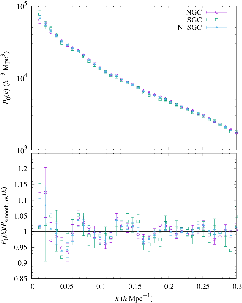
Figure 1: The measured power spectrum from the NGC, SGC, and their volume weighted average (top panel). To better see how they compare, they are also shown normalized by $P_{\mathrm{smooth,nw}}(k)$ as defined in equation (25) in the bottom panel (See the online article for a colour version of this plot.)

2.2 Measuring the Galaxy Bispectrum

We used the length of the three wave-vectors, $k_{1}$, $k_{2}$, and $k_{3}$, restricted by the triangle condition, $\mn@boldsymbol{k}_{1}+\mn@boldsymbol{k}_{2}+\mn@boldsymbol{k}_{3}=0$, to parametrize the shape of the bispectrum and averaged over two angles describing the orientation of the triangle (see e.g. Gil-Marín et al., 2015; Gagrani & Samushia, 2017). Since we were only using the monopole of the bispectrum we were able to use a Cartesian fast Fourier transform (FFT) without having to worry about the wide-angle effects (Samushia et al., 2015; Scoccimarro, 2015).

We employed a ‘brute-force’ algorithm that explicitly looked at all triplets that fell within a specific ($k_{1},k_{2},k_{3}$) bin and satisfied the triangle condition. This algorithm scales as $\mathcal{O}(N_{k}^{2})$ – where $N_{k}$ is the number of grid points in Fourier space where $k$ is in the range of interest.

It is possible to calculate the bispectrum using point-wise products of FFTs of shells of $\delta(k_{1})$, $\delta(k_{2})$ and $\delta(k_{3})$, with $\delta(k)$ being the FFT of the galaxy over-density field (see e.g. Baldauf et al., 2015, section 5.1). However, we found that it was computationally more efficient to use the ‘brute-force’ algorithm implemented on a graphics processor unit (GPU).

Our estimate of the bispectrum was (Scoccimarro, 2000; Scoccimarro et al., 2001)

$$\hat{B}(k_{1},k_{2},k_{3})=\dfrac{\left\{\langle\Re[\delta(\mn@boldsymbol{k}_{1})\delta(\mn@boldsymbol{k}_{2})\delta(\mn@boldsymbol{k}_{3})]\rangle-S_{\mathrm{B}}\right\}G(\mn@boldsymbol{k}_{1})G(\mn@boldsymbol{k}_{2})G(\mn@boldsymbol{k}_{3})}{\int\bar{n}^{3}(\mn@boldsymbol{r})w^{3}(\mn@boldsymbol{r})\mathrm{d}\mn@boldsymbol{r}}$$ (17)

where $\Re$ denotes the real part of a complex number and $\delta(\mn@boldsymbol{k})$ is the Fourier transformed over-density field used in the power spectrum calculation. The shotnoise $S_{\mathrm{B}}$, was computed using the power spectrum estimate of equation (11) (Scoccimarro, 2000; Scoccimarro et al., 2001)

$$S_{\mathrm{B}}=(\hat{P}_{1}+\hat{P}_{2}+\hat{P}_{3})\int\bar{n}^{2}(\mn@boldsymbol{r})w^{3}(\mn@boldsymbol{r})\mathrm{d}\mn@boldsymbol{r}+(1-\alpha^{2})\int\bar{n}(\mn@boldsymbol{r})w^{3}(\mn@boldsymbol{r})\mathrm{d}\mn@boldsymbol{r},$$ (18)

where $\hat{P}_{i}=\hat{P}(k_{i})$ is the estimate of the power spectrum at $k_{i}$. We computed the combined N+SGC bispectrum in the same way as we computed combined power spectrum, using the weights of equation (15) and simply replacing the power spectrum measurements in equation (16) with the bispectrum measurements.

To implement our estimator on the GPU, we first trimmed the Fourier transformed over-density field keeping only the wave numbers in our range of interest, $0.04\leq k<0.168$, to better fit in the limited memory resources of the GPUs used for the calculation. We then generated an array of $\mn@boldsymbol{k}$ values stored as integer multiples of the fundamental frequency in each coordinate direction. Each GPU thread took a single $\mn@boldsymbol{k}_{1}$ and looped over the other $\mn@boldsymbol{k}$’s as $\mn@boldsymbol{k}_{2}$, starting at $\mn@boldsymbol{k}_{1}$ and going through vectors not yet used as $\mn@boldsymbol{k}_{1}$, to avoid double counting. The value of $\mn@boldsymbol{k}_{3}$ was then computed from the triangle condition and checked to ensure it was in the range of interest.

For convenience and speed, we used the cuda types int4 and float4 (mocks) or double4 (data) for storing the $\mn@boldsymbol{k}$’s and the over-density field, respectively, allowing for four numbers of each type to be stored at a single array index. The int4 type allowed us to store the three components as well as the corresponding grid index for the over-density field, which made the lookup times negligible. For the over-density field, the first two values were the real and imaginary parts, the third value was the magnitude of $\mn@boldsymbol{k}$ at that grid point, and the fourth value was the correction for the CIC binning associated with that point.

As the GPUs used for this work had relatively low double-precision performance – really not much better than a typical CPU – to achieve high-throughput while retaining accuracy it was necessary to use mixed precision for calculating the bispectrum from the 2048 NGC and 2048 SGC mocks. Effectively, the calculation of $\mn@boldsymbol{k}_{3}$ was done as integer math, the overall grid-correction was calculated using single-precision, while the bispectrum contribution was calculated using single-precision, but stored and then binned as double-precision. The binning was done via a cuda function atomicAdd. While the double-precision version of this function is only supported on NVidia GPUs of compute capability 6 or higher, the documentation provides an implementation that can be used on GPUs of lower compute capabilities.

The reason it is not implemented on those older GPUs, however, is due to its relatively low performance, meaning that it was by far the most expensive step in the process. To reduce the impact of this step, the binning was first done in the GPU thread block shared memory, which is much lower latency than the global GPU memory. Once all of the threads in a block went through all of their $k_{2}$’s, the histogram was then binned into global memory in parallel. Naively, it may seem that the two step process would be less efficient, however, due to the lower latency of the shared memory, reduction in number of writes to global memory, and fewer bank conflicts, you can often see at least a factor of 2 speed up (Sakharnykh, 2015).

Implemented in this manner, we were able to compute the bispectrum from a single mock in $\sim$94 s, which was 15 to 20 times faster than our FFT based implementation, depending on whether a newer Intel core i7 or older AMD FX processor was used, respectively. Our full double precision implementation used for processing the data took $\sim$310 s. If we had used that implementation to process the mocks, it would have taken approximately 14.5 days to complete. Our mixed precision implementation cut that down to about 4.5 days.

We show the measured bispectrum from the NGC, SGC and N+SGC samples in Figure 2. We also show the measurements normalized by our best fitting model – see section 3.2 – to show that it is able to fit the data well.

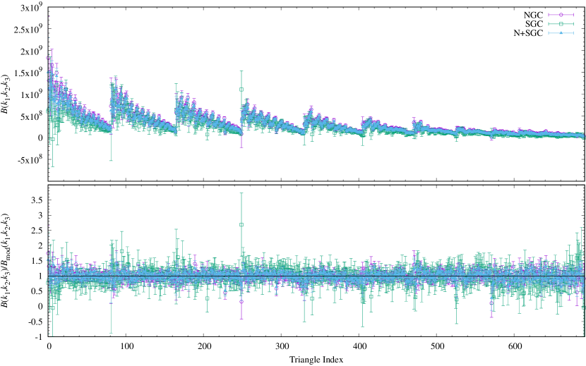
Figure 2: The measured bispectrum from the NGC, SGC, and N+SGC samples. The top panel shows the measurements with uncertainties ($\sqrt{C_{ii}}$) using the same symbols (and colours for the online version) as in Figure 1. The bottom panel shows the data normalized by the best fitting model. The fact that the normalized data are simply scattered about one shows that our model accounts for the non-linearities in the data quite well.

Unlike the power spectrum, the raw bispectrum measurements do not visibly show the BAO feature. To elucidate the type of signal our constraints come from, we provide a two-dimensional plot of the theoretical bispectrum calculated from a BAO power spectrum normalized by one calculated from a no-wiggle power spectrum as a function of two wave-vector magnitudes, averaged over the length of the third, in Figure 3 (see section 3.2). Plotted in this manner, it is possible to see clear hills and valleys coming from the BAO feature which are equivalent to the decaying oscillatory signature in the power spectrum.

Additionally, we used this plot, along with the need to keep the data vector small enough to ensure reasonable covariance matrices, to decide what bispectrum wave number range to use in our fits. The inset square (cyan in the online version) shows our selected region, which should include the equivalent of the first two ‘wiggles’ in the power spectrum, helping to maximize the BAO constraining power, while keeping the data vector reasonably sized. We note that this two-dimensional plot is merely a convenient way of displaying the BAO features in the bispectrum. Our actual constraints on the scale dilation parameter came from fitting to the three dimensional data shown in Figure 2.

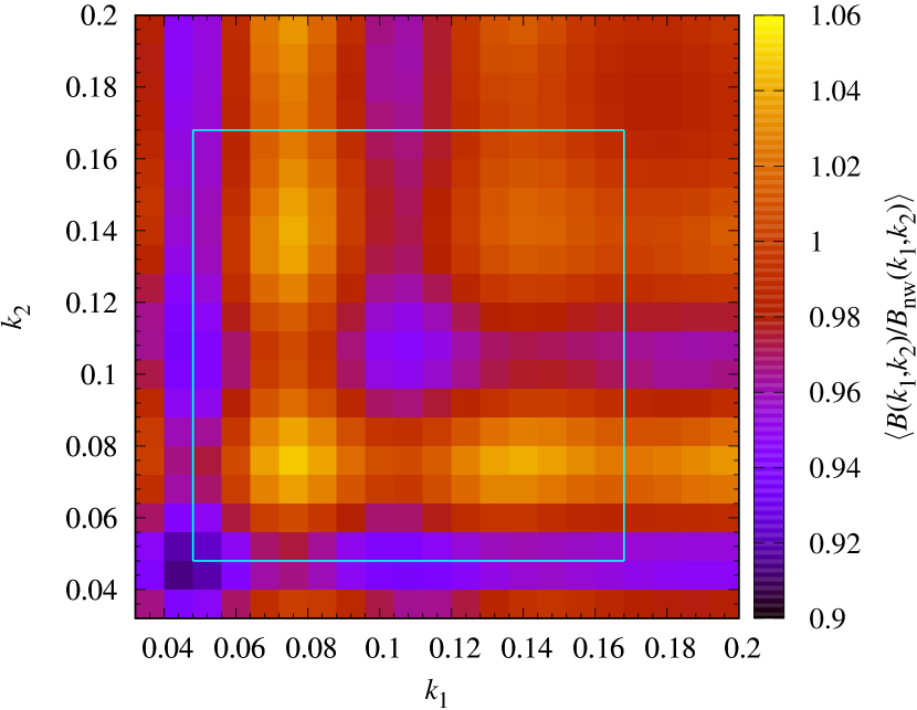
Figure 3: The theoretical bispectrum normalized by the theoretical no-wiggle bispectrum, as a function of the length of two wave-vectors, averaged over the length of the third wave-vector. The inset box (cyan in the online version) encloses the scales used in our analysis. The two dimensional sequence of local maxima and minima are manifestations of the BAO feature. (See the online article for a colour version of this plot.)

2.3 Covariance

We computed the sample covariance from the 2048 MultiDark-patchy mocks provided with DR12 (Kitaura et al., 2016; Rodríguez-Torres et al., 2016). This was the main limit to the number of triangles we could use for fitting the bispectrum data. First, we needed to estimate the covariance matrix to enough accuracy that it was not singular, if we were to invert it for our maximum likelihood fitting. Additionally, the errors in our covariance matrix carry through and affect our constraints on the model parameters. To ensure that the matrix was invertible, and that the uncertainties of its elements were kept low, we limited ourselves to $0.04\leq k_{1},k_{2},k_{3}\leq 0.168$ for the bispectrum measurements, and $0.008\leq k<0.304$ for the power spectrum. In total, we had 691 bispectrum triangles and 37 power spectrum points, which gave at most 728 elements in our data vector.

We ran all of the mocks through our data pipelines as described above, then computed the sample covariance,

$$C_{ij}=\dfrac{1}{n_{s}-1}\sum_{s}(x_{i}^{s}-\bar{x}_{i})(x_{j}^{s}-\bar{x}_{j}),$$ (19)

where $n_{s}$ is the number of mock samples, and the $s$ in the sum refers to a specific sample. We did this for the NGC, SGC and N+SGC samples with the power spectrum, bispectrum and both combined as our data vector, $\mn@boldsymbol{x}$. We plot the resulting correlation matrices, $r_{ij}=C_{ij}/(C_{ii}C_{jj})^{1/2}$, in Figures 4, and 5. All seem reasonably well behaved, with more than 90 per cent of the off-diagonal values falling between $\pm 0.2$.

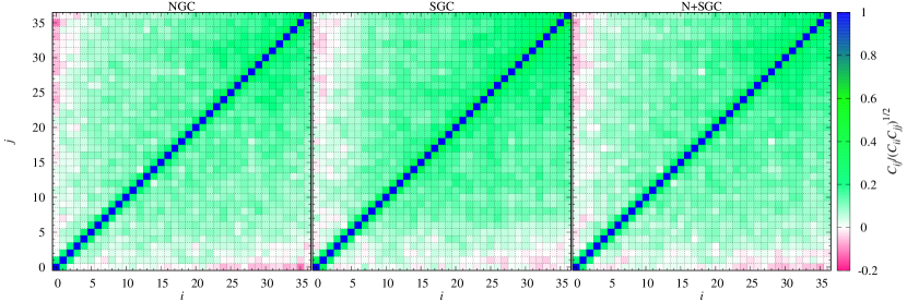
Figure 4: The correlation matrices for the power spectrum measurements calculated from 2048 Patchy mocks. The power spectra were calculated from the NGC and SGC, then a weighted average. Most of the off-diagonal values vary between $\pm 0.2$. (See the online article for a colour version of this plot.)

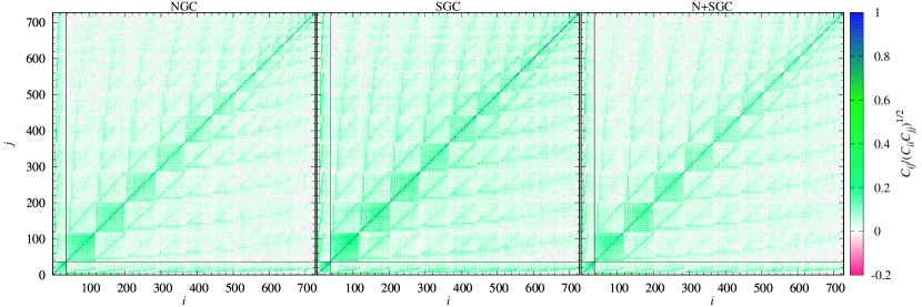
Figure 5: The correlation matrices for the power spectrum and bispectrum with cross-correlations calculated from the 2048 Patchy mocks. The vertical and horizontal solid lines divide the matrix into the power spectrum (bottom left, small square), the bispectrum (top right, large square), and their cross-correlations (vertical rectangle on the left, or horizontal rectangle on the bottom). The off-diagonal elements still mostly only vary between $\pm 0.2$. (See the online article for colour a version of this plot.)

When using the covariance matrix for our parameter fitting, we corrected for the fact that the inverse of the covariance matrix is a biased estimate of the true inverse covariance needed. This correction was simply (Hartlap et al., 2007; Percival et al., 2014)

$$\Psi=\left(\dfrac{n_{s}-n_{b}-2}{n_{s}-1}\right)\mn@boldsymbol{\mathsf{C}}^{-1}$$ (20)

where $n_{b}$ is the number of values in our data vector. Given that $n_{s}=2048$, and $n_{b}=37,~{}691$, and $728$ for the power spectrum, bispectrum, and combined data vectors, respectively, the above correction factor was then 0.981, 0.662, and 0.644, meaning our constraints on parameters from the bispectrum and the combined data were affected by the limited number of mock catalogues.

In addition to the correction above, we also had to carry through the uncertainty in the covariance matrix elements themselves due to limited number of mock catalogues (Taylor et al., 2013). This affected the variance of the parameters being constrained, increasing them by a factor of (Percival et al., 2014)

$$m_{1}=\dfrac{1+\beta(n_{b}-n_{p})}{1+A+\beta(n_{p}+1)},$$ (21)

where

$$A=\dfrac{2}{(n_{s}-n_{b}-1)(n_{s}-n_{b}-4)},$$ (22)

$$\beta=\dfrac{(n_{s}-n_{b}-2)}{(n_{s}-n_{b}-1)(n_{s}-n_{b}-4)},$$ (23)

and $n_{p}$ is the number of parameters in the model being fit to the data. For our analysis we found values of $m_{1}=1.0089,~{}1.4982$, and $1.5248$ for the power spectrum, bispectrum and combined sample, respectively. This substantially reduced the potential constraints from the bispectrum and the combined samples, highlighting a need for either a larger number of mock catalogues or a high precision theoretical model of the covariance.

3 Model & Fitting

3.1 The Power Spectrum

To model the power spectrum, we followed the method of Anderson et al. (2014), with one modification. We used the Python implementation of camb (Lewis et al., 2000) to generate a linear power spectrum with our fiducial cosmology. Then, using the fitting formula of Eisenstein & Hu (1998), we calculated a no-wiggle power spectrum to match the broadband shape of the linear power spectrum from camb. Since the data contained non-linearities, we used a smoothing polynomial to match the linear theory power spectrum to the data,

$$\mathcal{P}(k)=a_{0}k^{2}+a_{1}k+a_{2}+\dfrac{a_{3}}{k}+\dfrac{a_{4}}{k^{2}}+\dfrac{a_{5}}{k^{3}}.$$ (24)

This differs from the method used in Anderson et al. (2014) by including a term proportion to $k^{2}$. We found that including this extra term gives us a better fit. We added this polynomial to the no-wiggle power spectrum

$$P_{\mathrm{smooth,nw}}(k)=B^{2}P_{\mathrm{nw}}(k)+\mathcal{P}(k),$$ (25)

where $B$ is an amplitude parameter to account for galaxy bias and gravitational growth. This was then multiplied by an oscillatory part

$$O(k)=\left[1+\left(\dfrac{P_{\mathrm{lin}}(k/\alpha)}{P_{\mathrm{nw}}(k/\alpha)}-1\right)\exp\left(\dfrac{1}{2}\Sigma^{2}k^{2}\right)\right]$$ (26)

where $\alpha$ is defined in equation (1), and $\Sigma$ is a Finger-of-God damping parameter. This gave our final power spectrum model as

$$P_{\mathrm{mod}}(k)=P_{\mathrm{smooth,nw}}(k)O(k).$$ (27)

Figure 6 shows the average power spectrum of the 2048 mocks divided by the no-wiggle best fitting model – e.g. the average divided by equation (25) with the best fitting values of the parameters – as well as equation (26) with the best fitting parameter values.

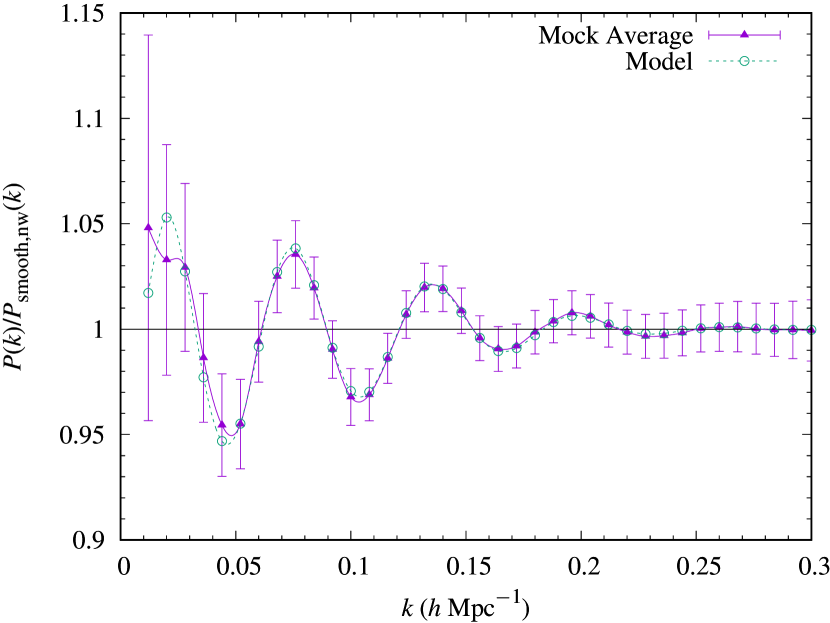
Figure 6: A comparison of the best fitting model and the average measured power spectrum from mock galaxy catalogues. The triangles show the mock average normalized by $P_{\mathrm{smooth,nw}}(k)$ defined in equation (25), calculated with the best fitting values of the $a_{i}$, and $B$ parameters, with a smooth cubic spline drawn through the points. The open circles show the model of equation (27) with the best fitting parameters normalized again by $P_{\mathrm{smooth,nw}}(k)$. The two agree quite well, particularly with respect to the BAO peak positions.

For the fitting, this model had 9 free parameters, the $a_{i}$ of equation (24), the amplitude parameter, $B$, the non-linear damping parameter, $\Sigma$, and the scale dilation parameter, $\alpha$. We used a custom Markov Chain Monte Carlo (MCMC) code which utilized the Metropolis-Hastings algorithm (Hastings, 1970). This choice was made so that when fitting simultaneously to the power spectrum and bispectrum, the exact same code and algorithm was used for both, as the bispectrum fitting had to be done with custom code in order to utilize a GPU to speed up the model calculation (see section 3.2).

3.2 The Bispectrum

To model the galaxy bispectrum we used the second-order perturbation theory model presented by Scoccimarro (2000), with some small changes to account for non-linearities in the data. The first and second-order kernels are

$$Z_{1}(\mn@boldsymbol{k})=(b_{1}+f\mu^{2})$$ (28)

and

$$\begin{array}[]{@{}l@{\:}l}Z_{2}(\mn@boldsymbol{k}_{1},\mn@boldsymbol{k}_{2})=\hfil\>&\dfrac{b_{2}}{2}+b_{1}F_{2}(\mn@boldsymbol{k}_{1},\mn@boldsymbol{k}_{2})+f\mu^{2}G_{2}(\mn@boldsymbol{k}_{1},\mn@boldsymbol{k}_{2})\\[4.30554pt] \hfil\>&+\dfrac{f\mu k}{2}\left[\dfrac{\mu_{1}}{k_{1}}Z_{1}(\mn@boldsymbol{k}_{2})+\dfrac{\mu_{2}}{k_{2}}Z_{1}(\mn@boldsymbol{k}_{1})\right],\end{array}$$ (29)

where $\mu\equiv\mn@boldsymbol{k}\cdot\hat{\mn@boldsymbol{z}}/k$, with $\mn@boldsymbol{k}\equiv\mn@boldsymbol{k}_{1}+\mn@boldsymbol{k}_{2}$, $\mu_{i}\equiv\mn@boldsymbol{k}_{i}\cdot\hat{\mn@boldsymbol{z}}/k_{i}$,

$$F_{2}(\mn@boldsymbol{k}_{1},\mn@boldsymbol{k}_{2})=\dfrac{5}{7}+\dfrac{\mn@boldsymbol{k}_{1}\cdot\mn@boldsymbol{k}_{2}}{2k_{1}k_{2}}\left(\dfrac{k_{1}}{k_{2}}+\dfrac{k_{2}}{k_{1}}\right)+\dfrac{2}{7}\left(\dfrac{\mn@boldsymbol{k}_{1}\cdot\mn@boldsymbol{k}_{2}}{k_{1}k_{2}}\right)^{2},$$ (30)

and

$$G_{2}(\mn@boldsymbol{k}_{1},\mn@boldsymbol{k}_{2})=\dfrac{3}{7}+\dfrac{\mn@boldsymbol{k}_{1}\cdot\mn@boldsymbol{k}_{2}}{2k_{1}k_{2}}\left(\dfrac{k_{1}}{k_{2}}+\dfrac{k_{2}}{k_{1}}\right)+\dfrac{4}{7}\left(\dfrac{\mn@boldsymbol{k}_{1}\cdot\mn@boldsymbol{k}_{2}}{k_{1}k_{2}}\right)^{2}.$$ (31)

From these, our model bispectrum was

$$\begin{array}[]{@{}l@{\;}l}B(\mn@boldsymbol{k}_{1},\mn@boldsymbol{k}_{2},\mn@boldsymbol{k}_{3})=&[2Z_{2}(\mn@boldsymbol{k}_{1},\mn@boldsymbol{k}_{2})Z_{1}(\mn@boldsymbol{k}_{1})Z_{1}(\mn@boldsymbol{k}_{2})P(k_{1})P(k_{2})\\ &+\;\mathrm{cyc.}]D_{\mathrm{FoG}}(\mn@boldsymbol{k}_{1},\mn@boldsymbol{k}_{2},\mn@boldsymbol{k}_{3}),\end{array}$$ (32)

where

$$D_{\mathrm{FoG}}(\mn@boldsymbol{k}_{1},\mn@boldsymbol{k}_{2},\mn@boldsymbol{k}_{3})=\dfrac{1}{1+(k_{1}^{2}\mu_{1}^{2}+k_{2}^{2}\mu_{2}^{2}+k_{3}^{2}\mu_{3}^{2})\sigma_{v}^{2}/2}$$ (33)

and $P(\mn@boldsymbol{k})$ is the non-linear power spectrum calculated for our fiducial cosmology from camb. The addition of the Finger-of-God suppression factor and the use of a non-linear power spectrum were the changes we made to better fit the data. Even though this model has been shown to be inadequate for fitting the full nonlinear bispectrum shape (Gil-Marín et al., 2015; Gil-Marín et al., 2017) we found it to be adequate for the range of $k$ that we consider (e.g. $0.04\leq k\leq 0.168$) in our analysis. Since we were only interested in the position of the BAO peak we could afford to marginalize over smooth systematic effects in the bispectrum shape without properly modelling them. We found that this was enough to get unbiased estimates of $\alpha$ and no extra smoothing polynomials seemed to be necessary to achieve a good fit to the bispectrum data.

Since we were examining the bispectrum monopole, equation (32) was spherically averaged by integrating over two angles: the angle of $\mn@boldsymbol{k}_{1}$ with the line of sight, $\mu_{1}$, and the azimuthal angle of $\mn@boldsymbol{k}_{2}$ around $\mn@boldsymbol{k}_{1}$, $\phi$ (see e.g. Gagrani & Samushia, 2017, section 3.1). This gave the model as

$$B(k_{1},k_{2},k_{3})=\dfrac{1}{4\pi}\int_{-1}^{1}\mathrm{d}\mu_{1}\int_{0}^{2\pi}\mathrm{d}\phi B(\mn@boldsymbol{k}_{1},\mn@boldsymbol{k}_{2},\mn@boldsymbol{k}_{3}).$$ (34)

The values of $\mu_{2}$ and $\mu_{3}$ could easily be calculated from the value of the two angles above. We took the Alcock-Paczynski effect (Alcock & Paczynski, 1979; Kaiser, 1987; Ballinger et al., 1996; Simpson & Peacock, 2010; Samushia et al., 2011) into account by transforming the measured $k$’s and $\mu$’s as

$$k_{i}\longrightarrow\dfrac{k_{i}}{\alpha_{\perp}}\left[1+\mu_{i}^{2}\left(\dfrac{\alpha_{\perp}^{2}}{\alpha_{\parallel}^{2}}-1\right)\right]^{1/2},$$ (35)

$$\mu_{i}\longrightarrow\dfrac{\alpha_{\perp}}{\alpha_{\parallel}}\mu_{i}\left[1+\mu_{i}^{2}\left(\dfrac{\alpha_{\perp}^{2}}{\alpha_{\parallel}^{2}}-1\right)\right]^{-1/2},$$ (36)

where

$$\alpha_{\parallel}=\dfrac{H^{\mathrm{fid}}(z)r_{\mathrm{d}}^{\mathrm{fid}}}{H(z)r_{\mathrm{d}}},$$ (37)

and

$$\alpha_{\perp}=\dfrac{D_{A}(z)r_{\mathrm{d}}^{\mathrm{fid}}}{D_{A}^{\mathrm{fid}}(z)r_{\mathrm{d}}},$$ (38)

along with renormalizing the power spectrum by a factor of $1/\alpha_{\perp}^{2}\alpha_{\parallel}$ and due to equation (32), the bispectrum by the same factor squared. From equations (1), (3), (37) and (38), it can be seen that $\alpha_{\parallel}$ and $\alpha_{\perp}$ are related to $\alpha$ via

$$\alpha^{3}=\alpha_{\perp}^{2}\alpha_{\parallel}.$$ (39)

Since the double-integral of equation (34) had to be evaluated for each of our 691 $k$-triplets a very large number of times for the MCMC fitting procedure, it had to be implemented in a numerically efficient manner. For this we again turned to the GPU allowing us to calculate the double-integral using a couple of levels of parallelism.

While it is possible to implement adaptive quadrature on the GPU, the error estimation steps can introduce significant overhead, and most algorithms rely on recursion which is not well suited for GPUs (Thuerck et al., 2014). Given this, we instead opted for the much easier to implement, fixed Gaussian quadrature rules. Since Gaussian quadrature can give an exact result for polynomials of degree $2n-1$ or less, it can allow very accurate numerical integration with relatively few function evaluations. Given that the exact shape of the above integrand can be difficult to predict, keeping $n$ as large as possible was desirable. Additionally, we again ran into the fact that commodity GPUs achieve the highest throughput for single precision floating point calculations. This made the use of mixed-precision necessary, where many of the calculations are done and variables stored as single precision floats.

Extending Gaussian quadrature in two-dimensions was done simply by setting up a two-dimensional grid such that

$$\int f(x,y)\mathrm{d}x\mathrm{d}y\cong\sum_{i=1}^{n}\sum_{j=1}^{n}w_{i}w_{j}f(x_{i},x_{j}),$$ (40)

where $x_{i}$ are the points to evaluate your function determined from your Gaussian quadrature rule, and $w_{i}$ are their associated weights, both of which can be readily found in handbooks. Combine the need for a two-dimensional grid, the unknown shape of the integrand, the need to use mixed precision and the fact that the maximum number of threads per GPU thread block is 1024, and $n=32$ becomes a natural choice.

This allowed us to have one thread block per $k$-triplet, where the integral was then approximated by a two-dimensional $32\times 32$-point Gaussian quadrature rule. Each thread then computed one contribution to the integral, and stored the result in block shared memory, with the final summing done in a two step reduction. To reduce the impact of mixed precision, we stored all the calculations of equations (28) – (31) as single precision and the calculations of equation (32) and (33) as double-precision. We then perform the final summing over the two-dimensional grid using those double-precision values and return the result as double-precision. In our tests, a complete double-precision calculation using the exact same algorithm has a relative difference – e.g. $(B_{\mathrm{MP}}-B_{\mathrm{DP}})/B_{\mathrm{DP}}$ – from our mixed-precision calculation of $\sim$10^-7. Given the relatively large uncertainties in the measured bispectrum, this loss of precision was well worth $\sim$12$\times$ speed-up of the model evaluation.

For the fitting, we used six free parameters: the three from equations (28) and (29), e.g. $b_{1}$, linear bias, $b_{2}$, second-order bias, and $f$, the linear growth factor with the two Alcock-Paczynski effect (Alcock & Paczynski, 1979; Kaiser, 1987; Ballinger et al., 1996; Simpson & Peacock, 2010; Samushia et al., 2011) parameters, $\alpha_{\parallel}$ and $\alpha_{\perp}$, and the Finger-of-God velocity dispersion parameter, $\sigma_{v}^{2}$. Since our model was only validated for the purposes of measuring the BAO feature we did not attach any cosmologically meaningful interpretation to the estimates of the parameters $b_{1}$, $b_{2}$, $f$, or $\sigma_{v}^{2}$. They were reasonably close to the linear model expectations but were very likely strongly affected by systematics and we therefore do not quote them as useful cosmological constraints in this work.

Since we were only fitting to the spherically averaged bispectrum monopole, we didn’t expect to be able to reliably constrain both $\alpha_{\parallel}$ and $\alpha_{\perp}$. Instead, as in the case of the spherically averaged two point statistics (see e.g. Anderson et al., 2012, 2014), we expected to only constrain the value of the single scale dilation parameter, $\alpha$. We elected to keep the fit in terms of $\alpha_{\parallel}$ and $\alpha_{\perp}$. Then we calculated the value of $\alpha$ via equation (39) for each of our accepted parameter realizations in the MCMC chain. It is not immediately obvious that the best constrained combination of $\alpha$s in the bispectrum is the same as for the power spectrum. By inspecting our MCMC chains we were able to verify that the two are in fact very close. Figure 7 shows one of our MCMC chains projected onto the $\alpha_{\parallel}$-$\alpha_{\perp}$ plane and the principle axis of the likelihood ellipse is very well aligned with the direction of $\alpha$ in equation (39).

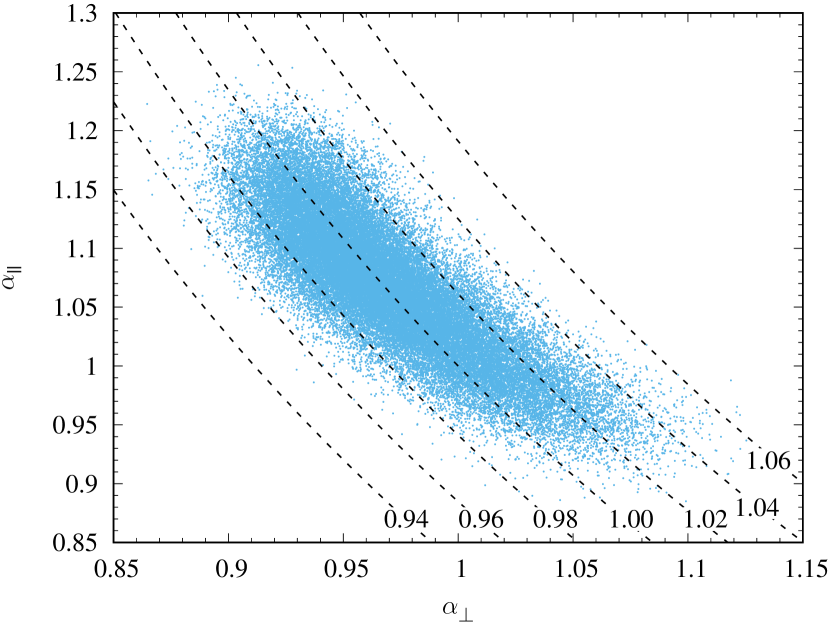
Figure 7: Accepted realizations from one of our MCMC chains fitting to the mock average N+SGC bispectrum projected onto $\alpha_{\parallel}$-$\alpha_{\perp}$ plane. The dashed lines correspond to fixed values of $\alpha^{3}\equiv\alpha_{\perp}^{2}\alpha_{\parallel}$.

We ran our MCMC chains with no priors aside from the loose requirement the $f$ remain positive. We used our own custom MCMC software utilizing the Metropolis-Hastings algorithm (Hastings, 1970), which was easier to interface with the model calculation on the GPU. Given that only one GPU was available for the model calculation and the GPU’s constant memory was used to store the values of the parameters for each model evaluation, we simply ran a single chain for many millions of realizations instead of running multiple, simultaneous chains needed to test for convergence. We built our code with the option to resume a chain should our post-processing reveal that it had not sufficiently explored the parameter space.

3.3 The Combined Power Spectrum and Bispectrum Model

For the joint fit our data vector simply became the 37 power spectrum values, followed by the 691 bispectrum values. The model was then simply calculating the first 37 values using the power spectrum model of section 3.1 and the next 691 values with the bispectrum model of section 3.2.

The main difference here came in the free parameters, particularly $\alpha$, $\alpha_{\perp}$ and $\alpha_{\parallel}$. Instead of letting all three be free, we instead only let $\alpha_{\perp}$ and $\alpha_{\parallel}$ vary freely with $\alpha$ for the power spectrum model then being fixed by equation (39). In all, for the combined model we ended up with 14 free parameters: $B$, $\Sigma$, $a_{0}$ – $a_{5}$, $b_{1}$, $b_{2}$, $f$, $\alpha_{\perp}$, $\alpha_{\parallel}$, and $\sigma_{\mathrm{v}}$. This likely could have been reduced by relating the power spectrum amplitude parameter $B$ to the biases, $b_{1}$ and $b_{2}$, and the linear growth factor, $f$. However, since we were only concerned with the constraints on $\alpha$ in the end, all other parameters were treated as nuisance parameters, and marginalized against anyway. We again ran our MCMC chains with only loose constraints to ensure that parameters that enter the models as squares remained positive.

4 Results

We performed a number of fittings to the power spectrum, bispectrum and their combination, analysing the NGC and SGC samples separately before fitting to the volume weighted averages. This was done to ensure that the results from any one fitting were consistent with the results from others. We additionally fit the models to the average power spectrum and bispectrum from the mock catalogues for the purposes of verifying our analysis pipeline and assessing systematic errors.

Our fiducial cosmology was virtually identical to that of the MultiDark-patchy mock catalogues. As such, we would expect that $\alpha$ should have been very nearly one when fit to the ensemble of mocks – the exact expected value is $\alpha_{\mathrm{mock}}=1.00005$. Looking at Table 1, we can see that this indeed turned out to be the case. We take the largest per cent deviation from the expected value of $\alpha$ for each of the fittings – e.g. the power spectrum, bispectrum and joint fittings – to indicate our systematic error. These errors were $\sim$0.7 per cent for the power spectrum and bispectrum, and $\sim$0.5 per cent for the combined fitting.

For the DR12 measurements, our results for the NGC and SGC separately are in agreement with Ross et al. (2017), who also analysed the NGC and SGC separately, finding a slightly lower value for the NGC and a slightly larger one for the SGC, and the combined result being closer to one. We also note the agreement of our power spectrum and bispectrum results. The largest difference is for the SGC measurements, which likely had to do with the smaller volume resulting in a noisier measurement of the bispectrum.

Table 1: The results of the MCMC fittings for the BAO scale parameter, $\alpha$. Both the values measured from the mocks and the data for the two galactic cap samples, as well as the volume weight averages, are presented. The standard deviations have been scaled due to the covariance uncertainty.

Data	Sample	$\alpha$ (mock)	$\alpha$ (DR12)
$P(k)$	NGC	$1.007\pm 0.018$	$0.976\pm 0.012$
	SGC	$1.003\pm 0.025$	$1.025\pm 0.021$
	N+SGC	$1.003\pm 0.013$	$0.988\pm 0.012$
$B(k_{1},k_{2},k_{3})$	NGC	$1.002\pm 0.020$	$0.978\pm 0.031$
	SGC	$1.007\pm 0.030$	$1.086\pm 0.072$
	N+SGC	$1.001\pm 0.017$	$0.991\pm 0.027$
$P(k)+B(k_{1},k_{2},k_{3})$	NGC	$1.001\pm 0.016$	$0.982\pm 0.011$
	SGC	$1.005\pm 0.020$	$1.020\pm 0.020$
	N+SGC	$1.002\pm 0.010$	$0.988\pm 0.011$

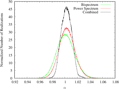
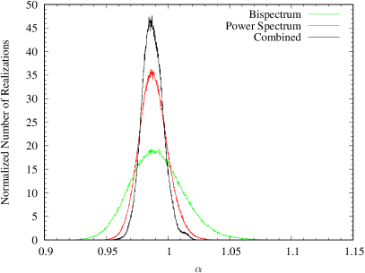
Figure 8: Histograms of the MCMC realizations from fitting to the bispectrum only, the power spectrum only, and the combination for the N+SGC. The left hand panel shows the results from fitting to the average of the mocks. The right hand panel shows the results from fitting to the measurments from the data. (See the online article for a colour version of this plot.)

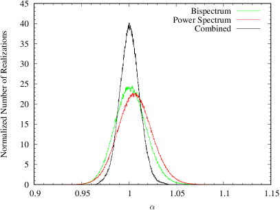
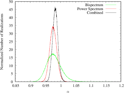
Figure 9: Histograms of the MCMC realizations from fitting to the bispectrum only, the power spectrum only, and the combination for the NGC CMASS sample. The panels are the same as in Figure 8. (See the online article for a colour version of this plot.)

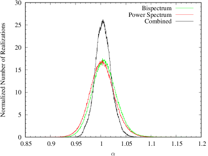
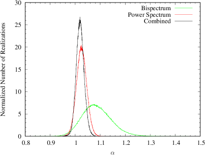
Figure 10: Histograms of the MCMC realizations from fitting to the bispectrum only, the power spectrum only, and the combination for the SGC CMASS sample. The panels are the same as in Figure 8. (See online article for colour version of this plot.)

We show the histograms for $\alpha$ from all of our MCMC fittings in Figures 8, 9, and 10 for the N+SGC, NGC, and SGC samples, respectively. In all of the figures, the results of fitting to the mocks is shown on the left, and the fitting to the data on the right, and all histograms have been normalized so that the area under the curves is equal to one. All of the histograms are very close to Gaussian and encapsulate all regions of relatively high likelihood suggesting that $\alpha$ parameter space was well explored by our MCMC chains. These plots have not been broadened by the $m_{1}$ factor of equation (21).

The standard deviations listed in Table 1 have been broadened by the $m_{1}$ factors. The effect is quite apparent in the full sample, N+SGC, combined power spectrum-bispectrum fitting. Without carrying the covariance uncertainty through, the standard deviation would be 0.0087, a $\sim$27 per cent tighter constraint than the power spectrum alone, and a better constraint than the one from the power spectrum of the reconstructed field. However, after multiplying by the square root of $m_{1}$, this become 0.0108 which still represents a $\sim$10 per cent tighter constraint than our power spectrum fitting.

To test how the constraints may improve given a more precise estimation of the covariance matrix, we ran chains fitting to the average of the mocks with the assumption that our covariance was drawn from one-million mock catalogues, which would make the effects both the covariance scaling and $m_{1}$ factor negligible. We did this for both the bispectrum and joint fitting, finding that the standard deviation for $\alpha$ dropped to 0.011 and 0.007 from 0.014 and 0.010, respectively. This indicates that given a less noisy estimate of the covariance, from either more mock catalogues, a high-precision theoretical calculation, or a hybrid approach like the one used by Slepian et al. (2017a, b), could improve constraints on the distance scale by 30 per cent.

We note that we achieve a significantly better fit by using a ‘wiggle’ power spectrum in our bispectrum model than a ‘no-wiggle’ power spectrum, with a $\chi^{2}$ penalty for the no-wiggle model of $\Delta\chi^{2}=20.64$. This implies a $4.1\sigma$ detection of the BAO features in the BOSS DR12 galaxy bispectrum, comparable to the significance of the detection by Slepian et al. (2017b).

Of course, $\alpha$ itself is merely a means to measure the distance to the survey redshift via equation (2). First it was necessary to compute $D_{\mathrm{V}}^{\mathrm{fid}}(z)$, which requires calculating $D_{\mathrm{A}}^{\mathrm{fid}}(z)$, and $H^{\mathrm{fid}}(z)$. For our fiducial cosmology, these come out to $H^{\mathrm{fid}}(z=0.57)=93.04~{}\mathrm{km}~{}\mathrm{s}^{-1}~{}\mathrm{Mpc}^{-1}$, $D_{\mathrm{A}}^{\mathrm{fid}}(z=0.57)=1386.01~{}\mathrm{Mpc}$, and $D_{\mathrm{V}}^{\mathrm{fid}}(z=0.57)=2056.45~{}\mathrm{Mpc}$. We also note that the drag radius for our fiducial cosmology was $r_{\mathrm{d}}^{\mathrm{fid}}=147.59~{}\mathrm{Mpc}$ as calculated from the fitting formula of Hu & Sugiyama (1996) and Eisenstein & Hu (1998). The values of $D_{\mathrm{V}}$ for the various fittings are reported in Table 2, where the $r_{\mathrm{d}}^{\mathrm{fid}}/r_{\mathrm{d}}$ was omitted from the column headings for brevity.

Table 2: The $D_{\mathrm{V}}$ values from the various fittings in Table 1. While the columns are labeled as $D_{\mathrm{V}}$ we note that they actually represent $(r_{\mathrm{d}}^{\mathrm{fid}}/r_{\mathrm{d}})D_{\mathrm{V}}$ values. The values for DR12 reported here agree remarkably well with the values reported by other analyses, and the values from the fittings to the mocks agree with our expectations.

Data	Sample	$D_{\mathrm{V}}$ (mock)	$D_{\mathrm{V}}$ (DR12)
		(Mpc)	(Mpc)
$P(k)$	NGC	$2070\pm 38$	$2007\pm 24$
	SGC	$2063\pm 51$	$2108\pm 42$
	N+SGC	$2063\pm 26$	$2032\pm 24$
$B(k_{1},k_{2},k_{3})$	NGC	$2060\pm 42$	$2012\pm 63$
	SGC	$2071\pm 62$	$2233\pm 148$
	N+SGC	$2059\pm 36$	$2038\pm 55$
$P(k)+B(k_{1},k_{2},k_{3})$	NGC	$2058\pm 27$	$2020\pm 23$
	SGC	$2066\pm 41$	$2097\pm 41$
	N+SGC	$2061\pm 21$	$2031\pm 22$

We take the measurement from the combined power spectrum plus bispectrum fitting to the N+SGC data as our main result,

$$D_{\mathrm{V}}(z=0.57)=2031\pm 22~{}\mathrm{Mpc}~{}\left(\dfrac{r_{\mathrm{d}}}{r_{\mathrm{d}}^{\mathrm{fid}}}\right).$$ (41)

We compared our result to that of other works to test its robustness, after converting those results to be consistent with our fiducial cosmology. Anderson et al. (2014) found

$$D_{\mathrm{V}}^{\mathrm{A14}}(z=0.57)=2032\pm 20~{}\mathrm{Mpc}~{}\left(\dfrac{r_{\mathrm{d}}}{r_{\mathrm{d}}^{\mathrm{fid}}}\right),$$ (42)

from their analysis of the DR11 CMASS sample. In analysing the DR12 CMASS sample Cuesta et al. (2016) found

$$D_{\mathrm{V}}^{\mathrm{C16}}(z=0.57)=2035\pm 20~{}\mathrm{Mpc}~{}\left(\dfrac{r_{\mathrm{d}}}{r_{\mathrm{d}}^{\mathrm{fid}}}\right),$$ (43)

Gil-Marín et al. (2016) found

$$D_{\mathrm{V}}^{\mathrm{G16}}(z=0.57)=2035\pm 19~{}\mathrm{Mpc}~{}\left(\dfrac{r_{\mathrm{d}}}{r_{\mathrm{d}}^{\mathrm{fid}}}\right),$$ (44)

Ross et al. (2017) found,

$$D_{\mathrm{V}}^{\mathrm{R17}}(z=0.57)=2022\pm 17~{}\mathrm{Mpc}~{}\left(\dfrac{r_{\mathrm{d}}}{r_{\mathrm{d}}^{\mathrm{fid}}}\right),$$ (45)

and Slepian et al. (2017b) found

$$D_{\mathrm{V}}^{\mathrm{S17m}}(z=0.57)=2036\pm 33~{}\mathrm{Mpc}~{}\left(\dfrac{r_{\mathrm{d}}}{r_{\mathrm{d}}^{\mathrm{fid}}}\right),$$ (46)

from their ‘minimal’ model and

$$D_{\mathrm{V}}^{\mathrm{S17t}}(z=0.57)=2026\pm 29~{}\mathrm{Mpc}~{}\left(\dfrac{r_{\mathrm{d}}}{r_{\mathrm{d}}^{\mathrm{fid}}}\right),$$ (47)

from their ‘tidal’ model. Our main result deviates the most from that of Ross et al. (2017), and even then the disagreement is within $\sim$0.5$\sigma$.

Additionally, Ross et al. (2017) gave results for the NGC and SGC separately, allowing for a more detailed comparison. Their fitting to the two-point correlation function gave

$$D_{\mathrm{V}}^{\mathrm{R17,NGC}}(z=0.57)=2006\pm 21~{}\mathrm{Mpc}~{}\left(\dfrac{r_{\mathrm{d}}}{r_{\mathrm{d}}^{\mathrm{fid}}}\right),$$ (48)

and

$$D_{\mathrm{V}}^{\mathrm{R17,SGC}}(z=0.57)=2090\pm 41~{}\mathrm{Mpc}~{}\left(\dfrac{r_{\mathrm{d}}}{r_{\mathrm{d}}^{\mathrm{fid}}}\right).$$ (49)

These values agree remarkably well with our analysis, showing a somewhat lower value from the NGC and a higher value from the SGC.

Similar to Slepian et al. (2017b), we assessed our systematic errors by examining the bias of our results of fitting to the mocks. We take the largest deviation from the expected value of $\alpha$ in each of the fittings, finding systematic errors of $\pm 15$ Mpc for the power spectrum and bispectrum fittings, and $\pm 10$ Mpc for the combined fitting. This gives our main result as

$$D_{\mathrm{V}}(z=0.57)=2031\pm 22~{}\mathrm{(stat.)}\pm 10~{}\mathrm{(sys.)}~{}\mathrm{Mpc}~{}\left(\dfrac{r_{\mathrm{d}}}{r_{\mathrm{d}}^{\mathrm{fid}}}\right).$$ (50)

5 Conclusions

We report an independent measurement of the distance to the BOSS DR12 CMASS sample of $D_{\mathrm{V}}(z=0.57)=2032\pm 24~{}\mathrm{Mpc}~{}(r_{\mathrm{d}}/r_{\mathrm{d}}^{\mathrm{fid}})$ from the power spectrum, $D_{\mathrm{V}}(z=0.57)=2038\pm 55~{}\mathrm{Mpc}~{}(r_{\mathrm{d}}/r_{\mathrm{d}}^{\mathrm{fid}})$ from the bispectrum, and $D_{\mathrm{V}}(z=0.57)=2031\pm 22~{}\mathrm{Mpc}~{}(r_{\mathrm{d}}/r_{\mathrm{d}}^{\mathrm{fid}})$ from the combined analysis. These values are in remarkable agreement with each other, and with the analyses of Anderson et al. (2014), Cuesta et al. (2016), Gil-Marín et al. (2016), Ross et al. (2017) and Slepian et al. (2017b). The power spectrum gives a $\sim$1.2 per cent constraint ($\sim$1.4 per cent with systematics), and the bispectrum gives a $\sim$2.7 per cent constraint ($\sim$2.8 per cent with systematics). The combined analyses gives a $\sim$1.1 per cent constraint ($\sim$1.2 per cent with systematics), mainly limited by the number mocks available for covariance estimation. However, when combined the constraint still improves by $~{}\sim$10 per cent compared to the power spectrum only constraints.

Our bispectrum constraints from the mocks were tighter than the ones from the data, suggesting that this specific realisation of the DR12 CMASS volume is slightly noisier than typical from the point of view of the bispectrum monopole estimator. When fitting to the mean of the mocks we get a 1.7 per cent constraint from the bispectrum only and a 1 per cent constraint from the joint fit to the power spectrum and bispectrum. The numbers in table 1 suggest that if a better model for the covariance were available the joint constraints from the power spectrum and the bispectrum would be comparable to the constraints from reconstructed power spectrum even at the current level of systematics.

The main limiting factor to the precision of the bispectrum measurements is a relatively small number of mock catalogues available for the covariance estimation. Having only 2048 mocks means that the values in our inverse covariance matrix estimate were all substantially reduced – by a factor of 0.662 for the bispectrum and 0.644 for the combined data – leading to broader posterior likelihoods. Having a better estimate of the bispectrum and joint covariance matrices would reduce the error on the $\alpha$ parameter from the joint fit by an extra $\sim$30 per cent. These improved estimates could come from either a larger number of mocks or analytic calculations.

Looking at Figure 11, we can clearly see that the power spectrum constraints will not really benefit from an increased number of mock catalogues, while the constraints from the bispectrum and the combined data can see dramatic improvements with $\sim$10 000 mocks. With $\sim$40 000 mocks, the additional uncertainty due to noise in the inverse covariance matrix would become negligible.

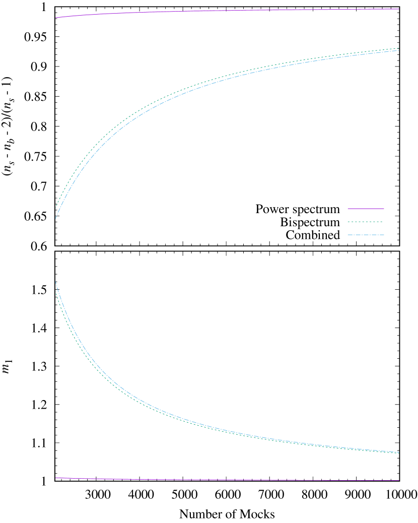
Figure 11: The effects of the limited number of mock catalogues. The top panel shows the factor that multiplies the inverse sample covariance, and the bottom panel shows how much the variance of parameter constraints should be inflated. The solid line (purple online) shows the quantities for the power spectrum, the dashed line (green online) shows them for the bispectrum, and the dot-dashed line (cyan online) shows them for the combined data vector. The horizontal axis starts at the number of mocks used in this work. It is clear that increasing the number of mocks will have little effect on the power spectrum, but a dramatic effect on bispectrum and combined data.

However, generating that number of mock catalogues is a computationally expensive proposition, which is only going to be exacerbated by the increased volumes and number densities of future redshift surveys such as, the upcoming DESI (Schlegel et al., 2011; Levi et al., 2013; DESI Collaboration et al., 2016) survey, Large Synoptic Survey Telescope (LSST; LSST Science Collaboration et al., 2009) surveys, Euclid satellite mission surveys (Laureijs et al., 2011), and WFIRST (Green et al., 2012) surveys. Monaco (2016) estimates that for these future surveys, generating 1000 mock realizations with the fastest of the popular mock codes currently in use would take $\sim$1 000 000 CPU hours since, unfortunately, the cheapest mock catalogues to produce, the lognormal mocks (Coles & Jones, 1991; Beutler et al.,, 2011; Pearson, Samushia & Gagrani, 2016), do not adequately reproduce the three-point statistics (see White et al., 2014, Figure 9).

It would also be interesting to test if various methods of reducing the uncertainties in the covariance matrix such as shrinkage estimation (Pope & Szapudi, 2008), estimation from fitting formula (Pearson & Samushia, 2016), or calculating the expected covariance from theory (Xu et al., 2012), could work for the bispectrum. Slepian et al. (2017a, b) used a hybrid approach, fitting a theoretical model to the sample covariance from a 299 mocks, which may also be a useful approach for the bispectrum.

Lastly, although we find our theoretical template to be unbiased for this analysis, it would be interesting to test if using a more complex bispectrum model, such as the one used by Gil-Marín et al. (2015) and Gil-Marín et al. (2017), would affect the constraints. We leave these matters for exploration in future works.

References

- Alam et al. (2017) Alam S., et al., 2017, MNRAS, 470, 2617
- Alcock & Paczynski (1979) Alcock C., Paczynski B., 1979, Nature, 281, 358
- Anderson et al. (2012) Anderson L., et al., 2012, MNRAS, 427, 3435
- Anderson et al. (2014) Anderson L., et al., 2014, MNRAS, 441, 24
- Baldauf et al. (2015) Baldauf T., Mercolli L., Mirbabayi M., Pajer E., 2015, J. Cosmology Astropart. Phys., 5, 007
- Ballinger et al. (1996) Ballinger W. E., Peacock J. A., Heavens A. F., 1996, MNRAS, 282, 877
- Beutler et al. (2011) Beutler F., et al., 2011, MNRAS, 416, 3017
- Beutler et al. (2017) Beutler F., et al., 2017, MNRAS, 464, 3409
- Coles & Jones (1991) Coles P., Jones B., 1991, MNRAS, 248, 1
- Cuesta et al. (2016) Cuesta A. J., et al., 2016, MNRAS, 457, 1770
- DESI Collaboration et al. (2016) DESI Collaboration et al., 2016, preprint, (arXiv:1611.00036)
- Dawson et al. (2013) Dawson K. S., et al., 2013, AJ, 145, 10
- Eisenstein & Hu (1998) Eisenstein D. J., Hu W., 1998, ApJ, 496, 605
- Eisenstein et al. (2007) Eisenstein D. J., Seo H.-J., Sirko E., Spergel D. N., 2007, ApJ, 664, 675
- Feldman et al. (1994) Feldman H. A., Kaiser N., Peacock J. A., 1994, ApJ, 426, 23
- Gagrani & Samushia (2017) Gagrani P., Samushia L., 2017, MNRAS, 467, 928
- Gil-Marín et al. (2015) Gil-Marín H., Noreña J., Verde L., Percival W. J., Wagner C., Manera M., Schneider D. P., 2015, MNRAS, 451, 539
- Gil-Marín et al. (2016) Gil-Marín H., et al., 2016, MNRAS, 460, 4210
- Gil-Marín et al. (2017) Gil-Marín H., Percival W. J., Verde L., Brownstein J. R., Chuang C.-H., Kitaura F.-S., Rodríguez-Torres S. A., Olmstead M. D., 2017, MNRAS, 465, 1757
- Green et al. (2012) Green J., et al., 2012, preprint, (arXiv:1208.4012)
- Hartlap et al. (2007) Hartlap J., Simon P., Schneider P., 2007, A&A, 464, 399
- Hastings (1970) Hastings W. K., 1970, Biometrika, 57, 97
- Hu & Sugiyama (1996) Hu W., Sugiyama N., 1996, ApJ, 471, 542
- Jeong (2010) Jeong D., 2010, PhD thesis, University of Texas at Austin
- Kaiser (1987) Kaiser N., 1987, MNRAS, 227, 1
- Kitaura et al. (2016) Kitaura F.-S., et al., 2016, MNRAS, 456, 4156
- LSST Science Collaboration et al. (2009) LSST Science Collaboration et al., 2009, preprint, (arXiv:0912.0201)
- Laureijs et al. (2011) Laureijs R., et al., 2011, preprint, (arXiv:1110.3193)
- Levi et al. (2013) Levi M., et al., 2013, preprint, (arXiv:1308.0847)
- Lewis et al. (2000) Lewis A., Challinor A., Lasenby A., 2000, ApJ, 538, 473
- Martínez & Saar (2002) Martínez V. J., Saar E., 2002, Statistics of the Galaxy Distribution. Chapman & Hall/CRC
- Monaco (2016) Monaco P., 2016, Galaxies, 4, 53
- Pearson & Samushia (2016) Pearson D. W., Samushia L., 2016, MNRAS, 457, 993
- Pearson et al. (2016) Pearson D. W., Samushia L., Gagrani P., 2016, MNRAS, 463, 2708
- Peebles (1980) Peebles P. J. E., 1980, The large-scale structure of the universe. Princeton University Press
- Percival et al. (2014) Percival W. J., et al., 2014, MNRAS, 439, 2531
- Planck Collaboration et al. (2016) Planck Collaboration et al., 2016, A&A, 594, A13
- Pope & Szapudi (2008) Pope A. C., Szapudi I., 2008, MNRAS, 389, 766
- Rodríguez-Torres et al. (2016) Rodríguez-Torres S. A., et al., 2016, MNRAS, 460, 1173
- Ross et al. (2017) Ross A. J., et al., 2017, MNRAS, 464, 1168
- Sakharnykh (2015) Sakharnykh N., 2015, GPU Pro Tip: Fast Histograms Using Shared Atomics on Maxwell, https://devblogs.nvidia.com/parallelforall/gpu-pro-tip-fast-histograms-using-shared-atomics-maxwell/ (Accessed on November 27, 2017)
- Samushia et al. (2011) Samushia L., et al., 2011, MNRAS, 410, 1993
- Samushia et al. (2015) Samushia L., Branchini E., Percival W. J., 2015, MNRAS, 452, 3704
- Schlegel et al. (2011) Schlegel D., et al., 2011, preprint, (arXiv:1106.1706)
- Scoccimarro (2000) Scoccimarro R., 2000, ApJ, 544, 597
- Scoccimarro (2015) Scoccimarro R., 2015, Phys. Rev. D, 92, 083532
- Scoccimarro et al. (2001) Scoccimarro R., Feldman H. A., Fry J. N., Frieman J. A., 2001, ApJ, 546, 652
- Sefusatti & Scoccimarro (2005) Sefusatti E., Scoccimarro R., 2005, Phys. Rev. D, 71, 063001
- Simpson & Peacock (2010) Simpson F., Peacock J. A., 2010, Phys. Rev. D, 81, 043512
- Slepian & Eisenstein (2015) Slepian Z., Eisenstein D. J., 2015, MNRAS, 454, 4142
- Slepian et al. (2017a) Slepian Z., et al., 2017a, MNRAS, 468, 1070
- Slepian et al. (2017b) Slepian Z., et al., 2017b, MNRAS, 469, 1738
- Spergel et al. (2015) Spergel D., et al., 2015, preprint, (arXiv:1503.03757)
- Taylor et al. (2013) Taylor A., Joachimi B., Kitching T., 2013, MNRAS, 432, 1928
- Thuerck et al. (2014) Thuerck D., Widmer S., Kuijper A., Goesele M., 2014, Efficient Heuristic Adaptive Quadrature on GPUs: Design and Evaluation. Springer Berlin Heidelberg, Berlin, Heidelberg, pp 652–662, doi:10.1007/978-3-642-55224-3_61, https://doi.org/10.1007/978-3-642-55224-3_61
- White et al. (2014) White M., Tinker J. L., McBride C. K., 2014, MNRAS, 437, 2594
- Xu et al. (2012) Xu X., Padmanabhan N., Eisenstein D. J., Mehta K. T., Cuesta A. J., 2012, MNRAS, 427, 2146