A long-term numerical energy-preserving analysis of symmetric and/or symplectic extended RKN integrators for efficiently solving highly oscillatory Hamiltonian systems

Abstract

The primary objective of this paper is to present a long-term numerical energy-preserving analysis of one-stage explicit symmetric and/or symplectic extended Runge–Kutta–Nyström (ERKN) integrators for highly oscillatory Hamiltonian systems. We study the long-time numerical energy conservation not only for symmetric integrators but also for symplectic integrators. In the analysis, we neither assume symplecticity for symmetric methods, nor assume symmetry for symplectic methods. It turns out that these both kinds of ERKN integrators have a near conservation of the total and oscillatory energy over a long term. To prove the result for symmetric integrators, a relationship between symmetric ERKN integrators and trigonometric integrators is established by using Strang splitting and based on this connection, the long-time conservation is derived. For the long-term analysis of symplectic ERKN integrators, the above approach does not work anymore and we use the technology of modulated Fourier expansion developed in SIAM J. Numer. Anal. 38 (2000) by Hairer and Lubich. By taking some novel adaptations of this essential technology for non-symmetric methods, we derive the modulated Fourier expansion for symplectic ERKN integrators. Moreover, it is shown that the symplectic ERKN integrators have two almost-invariants and then the near energy conservation over a long term is obtained.

Keywords: Long-time energy conservationModulated Fourier expansionsSymmetric or symplectic methodsExtended RKN integratorsHighly oscillatory Hamiltonian systems

MSC: 65P10, 65L05

1 Introduction

In this paper, we are concerned with the numerical energy-preserving analysis over a long term of extended Runge–Kutta–Nyström (ERKN) integrators when applied to the following highly oscillatory Hamiltonian system

$$\left\{\begin{aligned} &\dot{q}=\nabla_{p}H(q,p),\qquad\ \ q(0)=q^{0},\\ &\dot{p}=-\nabla_{q}H(q,p),\qquad p(0)=p^{0},\end{aligned}\right.$$ (1)

with the Hamiltonian

$$H(q,p)=\frac{1}{2}\big{(}\left\|p\right\|^{2}+\left\|\Omega q\right\|^{2}\big{)}+U(q),$$ (2)

where the vectors $p=(p_{1},p_{2})\in\mathbb{R}^{d_{1}}\times\mathbb{R}^{d_{2}}$ and $q=(q_{1},q_{2})\in\mathbb{R}^{d_{1}}\times\mathbb{R}^{d_{2}}$ are partitioned subject to the partition of the square matrix

$$\Omega=\left(\begin{array}[]{cc}0_{d_{1}\times d_{1}}&0_{d_{2}\times d_{2}}\\ 0_{d_{1}\times d_{1}}&\omega I_{d_{2}\times d_{2}}\\ \end{array}\right),$$ (3)

and $\omega$ is a large positive parameter. It is assumed in this paper that the initial values of (1) satisfy the condition

$$\frac{1}{2}\left\|p(0)\right\|^{2}+\frac{1}{2}\left\|\Omega q(0)\right\|^{2}\leq E,$$ (4)

where the constant $E$ is independent of $\omega$. As is known, the oscillatory energy of the system (1) is

$$I(q,p)=\frac{1}{2}p_{2}^{\intercal}p_{2}+\frac{1}{2}\omega^{2}q_{2}^{\intercal}q_{2}.$$ (5)

These highly oscillatory Hamiltonian systems frequently arise in a wide variety of applications including applied mathematics, quantum physics, classical mechanics, molecular biology, chemistry, astronomy, and electronics (see, e.g. [28, 30, 43, 46]). Over the past two decades (and earlier), some novel approaches have been extensively studied for the highly oscillatory Hamiltonian system and we refer the reader to [12, 19, 24, 29, 32, 33, 37, 39, 40] as well as the references contained therein.

The numerical long-time near-conservation of energy for such equations has already been researched for various numerical integrators, such as for symmetric trigonometric integrators in [6, 7, 22, 28], for the Störmer–Verlet method in [21], for an implicit-explicit method in [34, 36], and for heterogeneous multiscale methods in [35]. The essential technology used in the analysis is the modulated Fourier expansion, which was firstly developed in [22] to show long-time almost conservation properties of numerical methods for highly oscillatory Hamiltonian systems. A similar modulated Fourier expansion was independently presented in [20] on the spectral formulation of the Nekhoroshev theorem for quasi-integrable Hamiltonian systems. Following those pioneering researches, modulated Fourier expansions have been developed as an important mathematical tool in studying the long-time behaviour of numerical methods and differential equations (see, e.g. [4, 13, 14, 24, 25, 26, 31]). With this technology, much work has been done about different numerical methods for various systems. Besides the work stated above for the highly oscillatory Hamiltonian system (2), the numerical energy conservation for other kinds of systems has also been researched in many publications, such as for multi-frequency Hamiltonian systems in [8, 11], wave equations in [9, 10, 16, 23], Schrödinger equations in [5, 17, 18], highly oscillatory Hamiltonian systems without any non-resonance condition in [15], and Hamiltonian systems with a solution-dependent high frequency in [27].

On the other hand, in order to effectively solve (2) in the sense of structure-preservation, the authors in [45] formulated a standard form of extended Runge–Kutta–Nyström (ERKN) integrators and derived the corresponding order conditions by the B-series theory associated with the extended Nyström trees. In [41], the error bounds for explicit ERKN integrators were researched. Recently, symplecticity conditions of ERKN integrators were derived in [44] and symmetry conditions were derived in [46]. Based on these conditions, some practical symmetric or/and symplectic ERKN integrators were constructed and analyzed in [42]. The results of numerical experiments appearing in the work mentioned above have shown that the symmetric or/and symplectic ERKN integrators behave very well even in a long-time interval. However, the theoretical analysis of energy behaviour over a long term of symmetric or symplectic ERKN integrators has not been considered and researched yet in the literature, which motives this paper.

The main contributions of this work are to show the long-time energy behaviour not only for one-stage explicit symmetric ERKN integrators but also for symplectic ERKN integrators and to derive modulated Fourier expansions for non-symmetric methods. Similar results have been obtained for symmetric trigonometric integrators in [6, 8, 22, 28]. However, in this paper we prove the long-time result for more diverse methods than that for those considered previously. In particular, we present the analysis for both symmetric and symplectic ERKN integrators. We neither assume symplecticity for symmetric methods, nor assume symmetry for symplectic methods. It follows from the analysis that both symmetry and symplecticity can produce a good long-time energy conservation for ERKN integrators, which means that symmetry and symplecticity play a similar role in the numerical energy-preserving behaviour. This is a new discovery which is of great importance to geometric integration for highly oscillatory Hamiltonian systems. Moreover, in contrast to [6, 8, 22, 28], in the long-term analysis of symplectic integrators, the formulation of modulated Fourier expansions does not rely on the symmetry of the methods. This is of major importance in the context of long-term analysis of non-symmetric methods. It is also a main conceptual difference in comparison with [6, 8, 22, 28].

For the analysis of symmetric integrators, we have noted that some ERKN integrators can be formulated as a Strang splitting method applied to an averaged equation (see, [1]). Very recently, the authors in [2] proved second-order error bounds of trigonometric integrators on the basis of the interpretation of trigonometric integrators as splitting methods for averaged equations. Following this way, the long-term analysis of symmetric ERKN integrators will be proved concisely by exploring the connection between symmetric ERKN integrators and trigonometric integrators researched in [6, 8, 22, 28]. However, in the analysis of symplectic ERKN integrators, we do not require the symmetry of methods and it is known that the symmetry plays an important role in the construction of modulated Fourier expansions and long-term analysis given in [6, 8, 22, 28]. Therefore, unfortunately, the approach used for symmetric ERKN integrators does not apply to symplectic ERKN integrators any more. In order to overcome this difficulty, we will use the technology of modulated Fourier expansion developed by Hairer and Lubich in [22] with some novel adaptations for non-symmetric methods. The modulated Fourier expansion of symplectic ERKN integrators will be derived and two almost-invariants will be shown. Then the long-term result can be obtained.

This paper is organized as follows. We first present some preparatories of ERKN integrators in Section 2. The main results as well as an illustrative numerical experiment are given in Section 3. Then in Section 4, the result for symmetric integrators is proved by exploring the connection between symmetric ERKN integrators and trigonometric integrators and by using the previous results of symmetric trigonometric integrators shown in [6, 8, 22, 28]. Section 5 gives the proof of long-term result for symplectic ERKN integrators, where the modulated Fourier expansion is constructed for symplectic integrators and two almost-invariants of the modulated Fourier expansions are studied. The concluding remarks are made in the last section.

2 ERKN integrators

The highly oscillatory Hamiltonian system (2) can be rewritten as the following system of second-order differential equations

$$q^{\prime\prime}(t)+\Omega^{2}q(t)=g(q(t)),\qquad q(0)=q^{0},\ \ q^{\prime}(0)=p^{0},$$ (6)

where $g$ is the negative gradient of a real-valued function $U(q)$. ERKN integrators were first formulated for integrating (6) in [45] and here we summarize the scheme of one-stage ERKN integrators as follows.

Definition 2.1

(See [45]) A one-stage explicit ERKN integrator for solving (6) is defined by

$$\begin{array}[c]{ll}Q^{n+c_{1}}&=\phi_{0}(c_{1}^{2}V)q^{n}+hc_{1}\phi_{1}(c_{1}^{2}V)p^{n},\\ q^{n+1}&=\phi_{0}(V)q^{n}+h\phi_{1}(V)p^{n}+h^{2}\bar{b}_{1}(V)g(Q^{n+c_{1}}),\\ p^{n+1}&=-h\Omega^{2}\phi_{1}(V)q^{n}+\phi_{0}(V)p^{n}+h\textstyle b_{1}(V)g(Q^{n+c_{1}}),\end{array}$$ (7)

where $h$ is a stepsize, $c_{1}\in[0,1]$ is a real constant, $b_{1}(V)$ and $\bar{b}_{1}(V)$ are matrix-valued and bounded functions of $V\equiv h^{2}\Omega^{2}$, and

$$\phi_{j}(V):=\sum\limits_{k=0}^{\infty}\dfrac{(-1)^{k}V^{k}}{(2k+j)!},\qquad j=0,1.$$ (8)

From (8), it is clear that

$$\phi_{0}(V)=\cos(\sqrt{V})=\cos(h\Omega),\qquad\phi_{1}(V)=\sin(\sqrt{V})(\sqrt{V})^{-1}=\mathrm{sinc}(h\Omega),$$

where $\mathrm{sinc}(h\Omega)=\sin(h\Omega)(h\Omega)^{-1}.$ Thence the scheme of one-stage explicit ERKN integrators for (6) can be reformulated as follows.

Definition 2.2

The one-stage explicit ERKN integrator for integrating (6) is given by

$$Q^{n+c_{1}} =\cos(c_{1}h\Omega)q^{n}+c_{1}h\mathrm{sinc}(c_{1}h\Omega)p^{n},$$ (9)

$$q^{n+1} =\cos(h\Omega)q^{n}+h\mathrm{sinc}(h\Omega)p^{n}+h^{2}\bar{b}_{1}(h\Omega)g(Q^{n+c_{1}}),$$

$$p^{n+1} =-h\Omega^{2}\mathrm{sinc}(h\Omega)q^{n}+\cos(h\Omega)p^{n}+h\textstyle b_{1}(h\Omega)g(Q^{n+c_{1}}),$$

where the functions $\bar{b}_{1}(h\Omega)$ and $b_{1}(h\Omega)$ are real-valued and bounded functions of $h\Omega$.

As shown in [44, 46], we obtain the following conditions for the integrator (9) to be symmetric and symplectic.

Theorem 2.3

The ERKN integrator (9) is symmetric if and only if

$$c_{1}=1/2,\quad(I+\cos(h\Omega))\bar{b}_{1}(h\Omega)=\mathrm{sinc}(h\Omega)b_{1}(h\Omega).$$ (10)

Proof. It follows from the symmetry conditions given in [46] that this integrator is symmetric if and only if

$$c_{1}=1/2,\ \bar{b}_{1}(V)=\phi_{1}(V)b_{1}(V)-\phi_{0}(V)\bar{b}_{1}(V),$$ (11)

$$\phi_{0}(c_{1}^{2}V)\bar{b}_{1}(V)=c_{1}\phi_{1}(c_{1}^{2}V)b_{1}(V).$$

By solving the second equation in (LABEL:1s2con1), we obtain the second result of (LABEL:sym_cond). It can also be verified that under the condition (LABEL:sym_cond), the third equation of (LABEL:1s2con1) is true.

Theorem 2.4

For any real number $d_{1}$, if the coefficients are determined by

$$b_{1}(h\Omega)=d_{1}\cos((1-c_{1})h\Omega),\ \ \ \bar{b}_{1}(h\Omega)=d_{1}(1-c_{1})\mathrm{sinc}((1-c_{1})h\Omega),$$ (12)

then the ERKN integrator (9) is symplectic.

Proof. According to the symplectic conditions given in [44], we know that this method is symplectic if the following equations

$$\begin{array}[c]{ll}\phi_{0}(V)b_{1}(V)+V\phi_{1}(V)\bar{b}_{1}(V)=d_{1}\phi_{0}(c_{1}^{2}V),\ \ \ d_{1}\in\mathbb{R},\\ \phi_{1}(V)b_{1}(V)-\phi_{0}(V)\bar{b}_{1}(V)=c_{1}d_{1}\phi_{1}(c_{1}^{2}V),\end{array}$$

are satisfied. The result is directly obtained by solving these two equations.

Remark 2.5

These two theorems confirm the fact that an ERKN integrator can be symmetric and symplectic, or symmetric but not symplectic, or symplectic but not symmetric.

As some examples of ERKN integrators with certain structure characteristics, we present six practical one-stage explicit integrators and their coefficients are listed in Table 1. By Theorems 2.3 and 2.4, it can be verified that ERKN1 is neither symmetric nor symplectic, ERKN2 is symmetric and symplectic, ERKN3-4 are symmetric but not symplectic, and ERKN5-6 are symplectic but not symmetric.

$$\begin{array}[]{|c|c|c|c|c|c|c|c|}\hline\cr\text{Methods}&c_{1}&\bar{b}_{1}(h\omega)&b_{1}(h\omega)&\text{Symmetric}&\text{Symplectic}\\ \hline\cr\text{ERKN1}&\frac{1}{2}&\frac{1}{2}\textmd{sinc}^{2}(\frac{h\omega}{2})&\cos(\frac{h\omega}{2})&\text{Non}&\text{Non}\cr\text{ERKN1}&\frac{1}{2}&\frac{1}{2}\textmd{sinc}(\frac{h\omega}{2})&\cos(\frac{h\omega}{2})&\text{Symmetric}&\text{Symplectic}\cr\text{ERKN3}&\frac{1}{2}&\frac{1}{2}\textmd{sinc}(h\omega)\cos(\frac{h\omega}{2})&\cos^{3}(\frac{h\omega}{2})&\text{Symmetric}&\text{Non}\cr\text{ERKN4}&\frac{1}{2}&\frac{1}{2}\textmd{sinc}^{2}(\frac{h\omega}{2})&\textmd{sinc}(\frac{h\omega}{2})\cos(\frac{h\omega}{2})&\text{Symmetric}&\text{Non}\cr\text{ERKN5}&\frac{2}{5}&\frac{3}{5}\textmd{sinc}(\frac{3h\omega}{5})&\cos(\frac{3h\omega}{5})&\text{Non}&\text{Symplectic}\cr\text{ERKN6}&\frac{1}{5}&\frac{4}{5}\textmd{sinc}(\frac{4h\omega}{5})&\cos(\frac{4h\omega}{5})&\text{Non}&\text{Symplectic}\cr\hline\cr\end{array}$$

Table 1: Six one-stage explicit ERKN integrators.

3 Main results and numerical examples

Before presenting the main results of this paper, we make the following assumptions.

Assumption 3.1

• Assume that the initial values satisfy (4).

• The numerical solution is assumed to stay in a compact set.

• A lower bound on the stepsize is posed as:

  $$h\omega\geq c_{0}>0.$$ (13)

• The numerical non-resonance condition is assumed to be held

  $$|\sin(\frac{1}{2}kh\omega)|\geq c\sqrt{h}\ \ \mathrm{for}\ \ k=1,2,\ldots,N\ \ \mathrm{with}\ \ N\geq 2.$$ (14)

  For a given $h$ and $\omega$, this condition imposes a restriction on $N$. In the following, $N$ is a fixed integer such that (14) holds.

• For the coefficients of the ERKN integrators, it is assumed that the function

  $$\sigma(\nu)=\frac{\mathrm{sinc}(\nu)\cos(\frac{1}{2}\nu)}{2\bar{b}_{1}(\nu)}+\nu^{2}\mathrm{sinc}(\nu)\frac{\frac{1}{2}\mathrm{sinc}(\frac{1}{2}\nu)}{2b_{1}(\nu)}$$ (15)

  is bounded from below and above:

  $$0<c_{1}\leq\sigma(\nu)\leq C_{1}\quad\mathrm{for}\quad\nu=0,h\omega,$$ (16)

  or the same estimate holds for $-\sigma$ instead of $\sigma$.

It is noted that the first four assumptions are considered by many publications in the energy analysis of symmetric trigonometric integrators for the Hamiltonian system (1) (see, e.g. [4, 6, 22, 28]). The last assumption is obtained in the remainder analysis of this paper and it is similar to Assumption B proposed in [6].

With regard to the long-time total and oscillatory energy conservation along symmetric or symplectic ERKN integrators, we have the following two main results of this paper, which will be proved in detail in the next two sections, respectively.

Theorem 3.2

Under the conditions given in Assumption 3.1 and the symmetry condition (LABEL:sym_cond), for one-stage explicit symmetric ERKN integrators, it holds that

$$H(q^{n},p^{n}) =H(q^{0},p^{0})+\mathcal{O}(h),$$

$$I(q^{n},p^{n}) =I(q^{0},p^{0})+\mathcal{O}(h)$$

for $0\leq nh\leq h^{-N+1}.$ The constants symbolized by $\mathcal{O}$ depend on $N,T$ and the constants in the assumptions, but are independent of $n,\ h,\ \omega$.

Theorem 3.3

Under the conditions of Assumption 3.1 without the requirement (16) and the symplecticity condition (LABEL:symple_cond) with $d_{1}=1$, for one-stage explicit symplectic ERKN integrators, we have

$$H(q^{n},p^{n}) =H(q^{0},p^{0})+\mathcal{O}(h),$$

$$I(q^{n},p^{n}) =I(q^{0},p^{0})+\mathcal{O}(h),$$

where $0\leq nh\leq h^{-N+1}.$ The constants symbolized by $\mathcal{O}$ depend on $N,T$ and the constants in the assumptions, but are independent of $n,\ h,\ \omega$.

As an important nonlinear model, we consider the Fermi–Pasta–Ulam problem. This model describes classical and quantum systems of interacting particles in the physics of nonlinear phenomena. Denote by $x_{i}$ a scaled displacement of the $i$th stiff spring and by $x_{m+i}$ a scaled expansion or compression of the $i$th stiff spring. Their corresponding velocities are expressed in $y_{i}$ and $y_{m+i}$, respectively. Then the problem can be formulated by a Hamiltonian system with the Hamiltonian

$$\begin{array}[c]{ll}H(y,x)=&\dfrac{1}{2}\textstyle\sum\limits_{i=1}^{2m}y_{i}^{2}+\dfrac{\omega^{2}}{2}\textstyle\sum\limits_{i=1}^{m}x_{m+i}^{2}+\dfrac{1}{4}[(x_{1}-x_{m+1})^{4}\\ &+\textstyle\sum\limits_{i=1}^{m-1}(x_{i+1}-x_{m+i-1}-x_{i}-x_{m+i})^{4}+(x_{m}+x_{2m})^{4}].\end{array}$$

Following [28], we choose $m=3$ and

$$\ x_{1}(0)=1,\ y_{1}(0)=1,\ x_{4}(0)=\dfrac{1}{\omega},\ y_{4}(0)=1$$

with zero for the remaining initial values. First, the system is integrated in the interval $[0,10000]$ with $h=0.1$ and $\omega=50$. The errors of the total energy $H$ and oscillatory energy $I$ against $t$ for different ERKN integrators are shown in Fig. 1. Then we increase the size of $\omega$ to $200$ and see Fig. 2 for the results. It can be observed that the performance of ERKN1 is affected by $\omega$ and the corresponding errors become large as $\omega$ increases. However, the other methods are nearly not affected by $\omega$. Finally, we use a smaller stepsize $h=0.01$ and the results are presented in Figs. 3-4. Under this situation, all the methods behave better than the former.

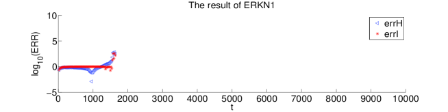
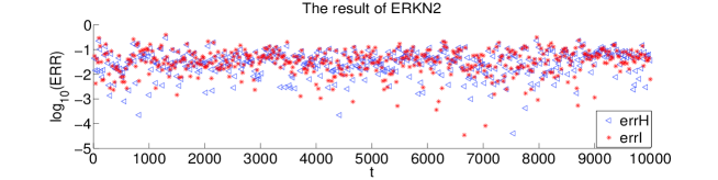
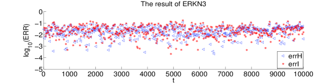
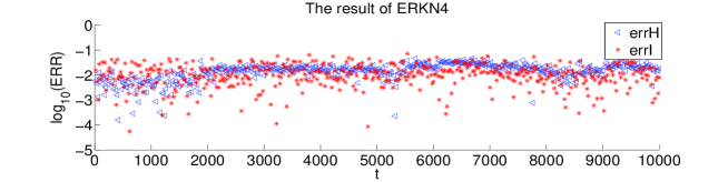
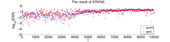
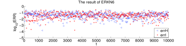
Figure 1: The logarithm of the errors ($ERR$) of $H$ and $I$ against $t$ with $h=0.1$ and $\omega=50$.

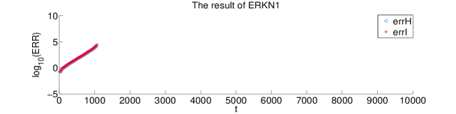
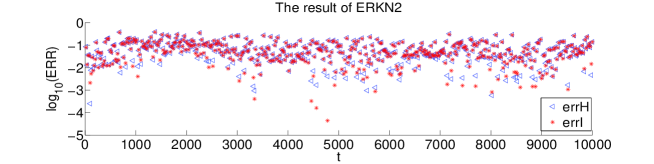
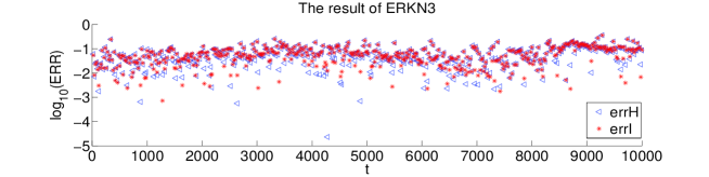
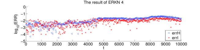
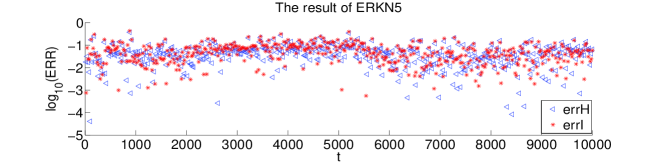
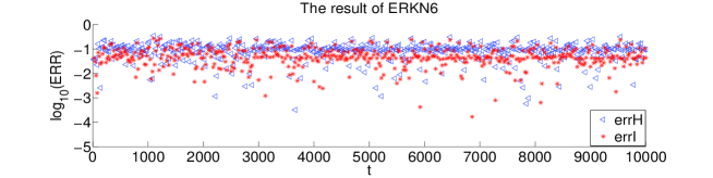
Figure 2: The logarithm of the errors ($ERR$) of $H$ and $I$ against $t$ with $h=0.1$ and $\omega=200$.

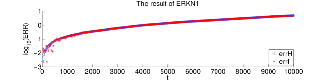
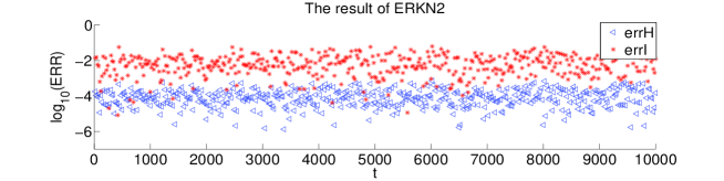
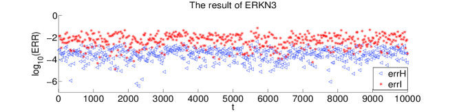
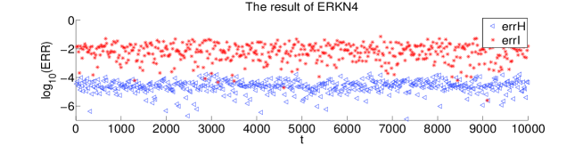
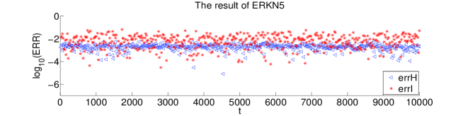
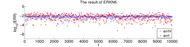
Figure 3: The logarithm of the errors ($ERR$) of $H$ and $I$ against $t$ with $h=0.01$ and $\omega=50$.

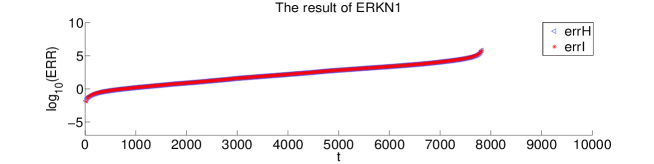
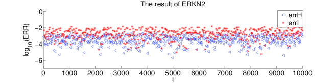
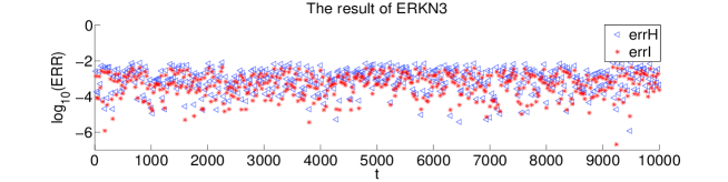
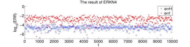
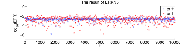
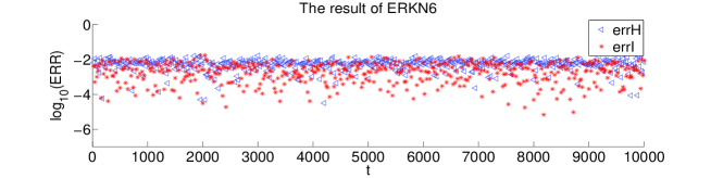
Figure 4: The logarithm of the errors ($ERR$) of $H$ and $I$ against $t$ with $h=0.01$ and $\omega=200$.

It follows from all the results that the integrators ERKN2-6 approximately conserve $H$ and $I$ quite well over a long term for different stepsizes and $\omega$. ERKN1 does not approximately conserve $H$ and $I$. In the light of the results, it seems that the symmetry or symplecticity is essential for the conservation of $H$ and $I$. All these numerical behaviours can be explained by the theoretical conclusions. According to Theorems 3.2 and 3.3, it can be concluded that if ERKN integrators are symmetric or symplectic, they have a near conservation of $H$ and $I$ over a long term. This is the theoretical reason for the behaviour shown in this numerical experiment.

4 Proof for symmetric integrators

In this section, we prove the result of long-time total and oscillatory energy conservation for symmetric ERKN integrators.

4.1 One important connection

We denote the numerical flow of a one-stage explicit symmetric ERKN integrator (9) with the symmetry condition (LABEL:sym_cond) by $\Phi_{h}$, i.e.,

$$(q^{n+1},p^{n+1})=\Phi_{h}(q^{n},p^{n}).$$

We now consider a Strang splitting applied to an averaged equation. More precisely, let $\Phi_{h,\textmd{L}}$ be the time $h$ flow of the linear equation $\frac{d}{dt}(q,p)=(p,\Omega^{2}q)$ and $\Phi_{h,\textmd{NL}}$ be the time $h$ flow of the nonlinear equation $\frac{d}{dt}(q,p)=(0,\Upsilon(h\Omega)g(q))$. We then consider the following Strang splitting method

$$\begin{array}[c]{ll}&\textmd{1. }(q_{+}^{n},p_{+}^{n})=\Phi_{h/2,\textmd{L}}(q^{n},p^{n}):\\ &\left(\begin{array}[]{c}q_{+}^{n}\\ p_{+}^{n}\\ \end{array}\right)=\left(\begin{array}[]{cc}\cos(\frac{h\Omega}{2})&\Omega^{-1}\sin(\frac{h\Omega}{2})\\ -\Omega\sin(\frac{h\Omega}{2})&\cos(\frac{h\Omega}{2})\\ \end{array}\right)\left(\begin{array}[]{c}q^{n}\\ p^{n}\\ \end{array}\right),\\ &\textmd{2. }(q_{-}^{n},p_{-}^{n})=\Phi_{h,\textmd{NL}}(q_{+}^{n},p_{+}^{n}):\\ &\left(\begin{array}[]{c}q_{-}^{n}\\ p_{-}^{n}\\ \end{array}\right)=\left(\begin{array}[]{c}q_{+}^{n}\\ p_{+}^{n}+h\Upsilon(h\Omega)g(q_{-}^{n})\\ \end{array}\right),\\ &\textmd{3. }(q^{n+1},p^{n+1})=\Phi_{h/2,\textmd{L}}(q_{-}^{n},p_{-}^{n}):\\ &\left(\begin{array}[]{c}q^{n+1}\\ p^{n+1}\\ \end{array}\right)=\left(\begin{array}[]{cc}\cos(\frac{h\Omega}{2})&\Omega^{-1}\sin(\frac{h\Omega}{2})\\ -\Omega\sin(\frac{h\Omega}{2})&\cos(\frac{h\Omega}{2})\\ \end{array}\right)\left(\begin{array}[]{c}q_{-}^{n}\\ p_{-}^{n}\\ \end{array}\right).\end{array}$$

It can be straightly verified that this Strang splitting method is identical to the ERKN integrator $\Phi_{h}$, i.e.,

$$\Phi_{h}=\Phi_{h/2,\textmd{L}}\circ\Phi_{h,\textmd{NL}}\circ\Phi_{h/2,\textmd{L}}$$ (17)

if and only if the following conditions hold

$$\frac{1}{2}\textmd{sinc}(\frac{1}{2}h\Omega)\Upsilon(h\Omega)=\bar{b}_{1}(h\Omega),\ \ \cos(\frac{1}{2}h\Omega)\Upsilon(h\Omega)=b_{1}(h\Omega).$$ (18)

For general ERKN integrators, these two conditions may not hold simultaneously. However, it is noted that under the symmetry condition (LABEL:sym_cond), (18) is true. In this particular case, the function $\Upsilon$ has the form

$$\Upsilon(h\Omega)=b_{1}(h\Omega)\cos^{-1}(\frac{1}{2}h\Omega)=2\bar{b}_{1}(h\Omega)\textmd{sinc}^{-1}(\frac{1}{2}h\Omega).$$ (19)

On the other hand, if we consider the Strang splitting in another way:

$$\hat{\Phi}_{h}=\Phi_{h/2,\textmd{NL}}\circ\Phi_{h,\textmd{L}}\circ\Phi_{h/2,\textmd{NL}},$$

which yields a class of trigonometric integrators

$$\begin{array}[c]{ll}&q^{n+1}=\cos(h\Omega)q^{n}+h\textmd{sinc}(h\Omega)p^{n}+\frac{1}{2}h^{2}\textmd{sinc}(h\Omega)\Upsilon(h\Omega)g(q^{n}),\\ &p^{n+1}=-\Omega\sin(h\Omega)q^{n}+\cos(h\Omega)p^{n}+\frac{1}{2}h\big{(}\cos(h\Omega)\Upsilon(h\Omega)g(q^{n})+\Upsilon(h\Omega)g(q^{n+1})\big{)}.\end{array}$$ (20)

It is noted that this is exactly a trigonometric integrator (a form of (XIII.2.7)-(XIII.2.8) given on p.481 of [28]) with the following coefficients

$$\begin{array}[c]{ll}\Phi(h\Omega)=1,\qquad\Psi(h\Omega)=\textmd{sinc}(h\Omega)\Upsilon(h\Omega),\\ \Psi_{0}(h\Omega)=\cos(h\Omega)\Upsilon(h\Omega),\ \ \Psi_{1}(h\Omega)=\Upsilon(h\Omega).\end{array}$$ (21)

In terms of the symmetry condition proposed in [28], it is clear that this trigonometric integrator is symmetric.

On the basis of the above analysis, the following important connection between symmetric ERKN integrators and symmetric trigonometric integrators is obtained.

Proposition 4.1

For the one-stage explicit symmetric ERKN integrator (9) and the symmetric trigonometric integrator (20), they are related by

$$\Phi_{h}=\Phi_{-h/2,\textmd{L}}\circ\Phi_{-h/2,\textmd{NL}}\circ\hat{\Phi}_{h}\circ\Phi_{h/2,\textmd{NL}}\circ\Phi_{h/2,\textmd{L}}.$$ (22)

The function $\Upsilon$ appearing in the averaged equation and in (21) is determined by (19). Moreover, it is true that

$$\underbrace{\Phi_{h}\circ\cdots\circ\Phi_{h}}_{n\ \textmd{times}}= \Phi_{-h/2,\textmd{L}}\circ\Phi_{-h/2,\textmd{NL}}\circ\big{(}\underbrace{\hat{\Phi}_{h}\circ\cdots\circ\hat{\Phi}_{h}}_{n\ \textmd{times}}\big{)}\circ\Phi_{h/2,\textmd{NL}}\circ\Phi_{h/2,\textmd{L}}$$ (23)

$$= \Phi_{h/2,\textmd{L}}\circ\Phi_{h/2,\textmd{NL}}\circ\big{(}\underbrace{\hat{\Phi}_{h}\circ\cdots\circ\hat{\Phi}_{h}}_{n-1\ \textmd{times}}\big{)}\circ\Phi_{h/2,\textmd{NL}}\circ\Phi_{h/2,\textmd{L}}.$$

4.2 Proof of Theorem 3.2

Since the long-time behaviour of symmetric trigonometric integrators is well understood (see [6, 22, 28]), the long-time near conservation of total and oscillatory energy of one-stage explicit symmetric ERKN integrators can be derived by using the relation (23). To be very precise, according to the analysis of [6, 22, 28], one has to verify the following four key points.

• I. If $(q^{0},p^{0})$ satisfies (4), the following initial value

  $$(\tilde{q}^{0},\tilde{p}^{0}):=\Phi_{h/2,\textmd{NL}}\circ\Phi_{h/2,\textmd{L}}(q^{0},p^{0})$$

  for $\big{(}\underbrace{\hat{\Phi}_{h}\circ\cdots\circ\hat{\Phi}_{h}}_{n-1\ \textmd{times}}\big{)}$ satisfies the finite-energy condition

  $$\frac{1}{2}\left\|\tilde{p}^{0}\right\|^{2}+\frac{1}{2}\left\|\Omega\tilde{q}^{0}\right\|^{2}\leq E.$$ (24)

• II. For any $j\in\mathbb{N}^{+}$, $\big{(}\underbrace{\hat{\Phi}_{h}\circ\cdots\circ\hat{\Phi}_{h}}_{j\ \textmd{times}}\big{)}\circ\Phi_{h/2,\textmd{NL}}\circ\Phi_{h/2,\textmd{L}}(q^{0},p^{0})$ stays in a compact set if $\big{(}\underbrace{\Phi_{h}\circ\cdots\circ\Phi_{h}}_{j\ \textmd{times}}\big{)}(q^{0},p^{0})$ does.

• III. The two additional steps with $\Phi_{h/2,\textmd{L}}$ and $\Phi_{h/2,\textmd{NL}}$ only introduce an $\mathcal{O}(h)$ deviation in the total and oscillatory energy, provided that the corresponding initial values $(\tilde{q},\tilde{p})$ are bounded and also $\Omega\tilde{q}$ is bounded.

• IV. The condition of [6] on $\Phi$ and $\Psi$ has to be satisfied for the choice (21).

In what follows, we show that the above four conditions are completely true.

• For the point I, according to the splitting method, it is easy to obtain that

  $$\tilde{q}^{0}=\cos(\frac{h\Omega}{2})q^{0}+\Omega^{-1}\sin(\frac{h\Omega}{2})p^{0},$$

  $$\tilde{p}^{0}=-\Omega\sin(\frac{h\Omega}{2})q^{0}+\cos(\frac{h\Omega}{2})p^{0}+\frac{1}{2}h\Upsilon(\frac{h\Omega}{2})g(\tilde{q}^{0}).$$

  Thus (24) is clear by considering (4).

• It follows from (22) that

  $$\big{(}\underbrace{\hat{\Phi}_{h}\circ\cdots\circ\hat{\Phi}_{h}}_{j\ \textmd{times}}\big{)}\circ\Phi_{h/2,\textmd{NL}}\circ\Phi_{h/2,\textmd{L}}(q^{0},p^{0})$$

  $$=\Phi_{h/2,\textmd{NL}}\circ\Phi_{h/2,\textmd{L}}\circ\big{(}\underbrace{\Phi_{h}\circ\cdots\circ\Phi_{h}}_{j\ \textmd{times}}\big{)}(q^{0},p^{0}),$$

  which gives the statement of II.

• The third result is clear in the light of the definitions of $\Phi_{h/2,\textmd{L}}$ and $\Phi_{h/2,\textmd{NL}}$.

• We remark that the long-term analysis of [22, 28] requires

  $$|\Phi(h\omega)|\geq C|\textmd{sinc}(\frac{1}{2}h\omega)|.$$

  However, for the trigonometric integrator (20) with $\Phi=1$, it does not satisfy the above requirement. Therefore, the long-term analysis of [22, 28] can not be used here. Recently, the authors in [6] improved the analysis and presented a long-term analysis of numerical integrators for oscillatory Hamiltonian systems under minimal non-resonance conditions. A more relaxed restriction on $\Phi$ was given there. In terms of that restriction and the relations (18) and (22), the statement of IV holds provided (16) is true.

Based on the above analysis and the long-time result of symmetric trigonometric integrators given in [6, 22, 28], Theorem 3.2 is immediately obtained.

5 Proof for symplectic integrators

In this section, we are devoted to the analysis of long-time conservation of the total and oscillatory energy along symplectic ERKN integrators. To do this, we begin with defining the operators

$$\begin{array}[c]{ll}\mathcal{L}_{1}(hD)=&\big{(}e^{hD}-\cos(h\Omega)-h^{2}\Omega^{2}\mathrm{sinc}(h\Omega)\bar{b}_{1}(h\Omega)b^{-1}_{1}(h\Omega)\big{)}\\ &\big{(}\bar{b}_{1}(h\Omega)b^{-1}_{1}(h\Omega)(e^{hD}-\cos(h\Omega))+\mathrm{sinc}(h\Omega)\big{)}^{-1},\\ \mathcal{L}_{2}(hD)=&\cos(c_{1}h\Omega)+c_{1}\mathrm{sinc}(c_{1}h\Omega)\mathcal{L}_{1}(hD),\\ \mathcal{L}(hD)=&\big{(}e^{hD}-\cos(h\Omega)-\mathrm{sinc}(h\Omega)\mathcal{L}_{1}(hD)\big{)}(\bar{b}_{1}(h\Omega)\mathcal{L}_{2}(hD))^{-1},\end{array}$$

where $D$ is the differential operator (see [27]). The following property will be used in this section.

Proposition 5.1

Under the symplecticity condition (LABEL:symple_cond) with $d_{1}=1$ of one-stage explicit ERKN integrators, the operator $\mathcal{L}(hD)$ can be simplified as

$$\mathcal{L}(hD)=-2h\Omega(\cos(h\Omega)-\cosh(hD))\csc(h\Omega).$$

Moreover, the Taylor expansions of the operator $\mathcal{L}(hD)$ are

$$\mathcal{L}(hD)= 2h\Omega\tan(\frac{1}{2}h\Omega)+h\Omega\csc(h\Omega)(hD)^{2}+\cdots,$$

$$\mathcal{L}(hD+\mathrm{i}h\omega)= \left(\begin{array}[]{cc}-4\sin^{2}(\frac{1}{2}h\omega))&\\ &0\\ \end{array}\right)+\left(\begin{array}[]{cc}2\sin(h\omega)&\\ &2h\omega\\ \end{array}\right)(\mathrm{i}hD)+\cdots,$$

$$\mathcal{L}(hD+\mathrm{i}kh\omega)= -4h\Omega\csc(h\Omega)\sin\big{(}\frac{kh\omega I+h\Omega}{2}\big{)}\sin\big{(}\frac{kh\omega I-h\Omega}{2}\big{)}$$

$$+2h\Omega\csc(h\Omega)\sin(kh\omega)(\mathrm{i}hD)+\cdots,\ \textmd{where}\ \left|k\right|>1.$$

5.1 Modulated Fourier expansion

We now derive the modulated Fourier expansions of symplectic ERKN integrators and present the bounds of the modulated Fourier functions.

Theorem 5.2

Under the conditions of Theorem 3.3 and for $0\leq t=nh\leq T$, the numerical solution of the one-stage explicit symplectic ERKN integrator (9) admits the following modulated Fourier expansions

$$q^{n}=\sum\limits_{|k|<N}\mathrm{e}^{\mathrm{i}k\omega t}\zeta_{h}^{k}(t)+R_{h,N}(t),$$ (25)

$$p^{n}=\sum\limits_{|k|<N}\mathrm{e}^{\mathrm{i}k\omega t}\eta_{h}^{k}(t)+S_{h,N}(t),$$

where the remainder terms are bounded by

$$R_{h,N}(t)=\mathcal{O}(th^{N}),\ \ \ \ S_{h,N}(t)=\mathcal{O}(th^{N-1}).\\$$ (26)

The coefficient functions $\zeta_{h}^{k}$ as well as all their derivatives are bounded by

$$\begin{array}[]{ll}\ddot{\zeta}^{0}_{h,1}=\mathcal{O}(1),\quad\ \zeta_{h,1}^{1}=\mathcal{O}(h^{2}),\ \ \zeta_{h,1}^{k}=\mathcal{O}(h^{\left|k\right|+1}),\\ \zeta^{0}_{h,2}=\mathcal{O}(h^{\frac{3}{2}}),\ \ \dot{\zeta}_{h,2}^{1}=(h),\quad\ \ \ \zeta_{h,2}^{k}=\mathcal{O}(h^{\left|k\right|+1}),\end{array}$$ (27)

for $\left|k\right|>1$ and further bounded by

$$\zeta^{0}_{h,1}=\mathcal{O}(1),\quad\ \ \zeta_{h,2}^{1}=\mathcal{O}(h).$$ (28)

Moreover, we have the following results for coefficient functions $\eta_{h}^{k}$

$$\begin{array}[]{ll}\eta_{h,1}^{0}=\dot{\zeta}_{h,1}^{0}+\mathcal{O}(h),\ \ \eta_{h,1}^{1}=\mathcal{O}(h),\qquad\qquad\ \eta_{h,1}^{k}=\mathcal{O}(h^{\left|k\right|}),\\ \eta_{h,2}^{0}=\mathcal{O}(h^{\frac{1}{2}}),\qquad\quad\eta_{h,2}^{1}=\mathrm{i}\omega\zeta_{h,2}^{1}+\mathcal{O}(h),\ \ \eta_{h,2}^{k}=\mathcal{O}(h^{\left|k\right|}),\end{array}$$ (29)

where $\left|k\right|>1$. Moreover, we have $\zeta^{-k}=\overline{\zeta^{k}}$ and $\eta^{-k}=\overline{\eta^{k}}$. The constants symbolized by the notation are independent of $h$ and $\omega$, but depend on the constants from Assumption 3.1 and the final time $T$.

Proof. The proof follows that used in the modulated Fourier expansions of previous publications (see [6, 8, 22, 28]) but with some novel adaptations for non-symmetric methods. The proof of this theorem does not rely on the symmetry of the methods, which is a main conceptual difference in comparison with that in [6, 8, 22, 28].

We will prove that there exist two functions

$$q_{h}(t)=\sum\limits_{|k|<N}\mathrm{e}^{\mathrm{i}k\omega t}\zeta_{h}^{k}(t),\ \ p_{h}(t)=\sum\limits_{|k|<N}\mathrm{e}^{\mathrm{i}k\omega t}\eta_{h}^{k}(t)$$ (30)

with smooth (in the sense that all their derivatives are bounded independently of $h$ and $\omega$) coefficients $\zeta_{h}^{k},\eta_{h}^{k}$, such that, for $t=nh$,

$$q^{n}=q_{h}(t)+\mathcal{O}(h^{N}),\qquad p^{n}=p_{h}(t)+\mathcal{O}(h^{N-1}).$$

Construction of the coefficients functions. According to the second and third formulae of (9), it is arrived that

$$q^{n+1}-\big{(}\cos(h\Omega)+h^{2}\Omega^{2}\mathrm{sinc}(h\Omega)\bar{b}_{1}(h\Omega)b^{-1}_{1}(h\Omega)\big{)}q^{n}$$

$$= h\bar{b}_{1}(h\Omega)b^{-1}_{1}(h\Omega)p^{n+1}+h\big{(}\mathrm{sinc}(h\Omega)-\bar{b}_{1}(h\Omega)b^{-1}_{1}(h\Omega)\cos(h\Omega)\big{)}p^{n}.$$

Comparing the coefficients of $\mathrm{e}^{\mathrm{i}k\omega t}$ and considering the definition of $\mathcal{L}_{1}$ implies the relationship between $\zeta_{h}^{k}$ and $\eta_{h}^{k}$ as follows:

$$\mathcal{L}_{1}(hD)\zeta_{h}^{0}=h\eta_{h}^{0},$$ (31)

$$\mathcal{L}_{1}(hD+\mathrm{i}kh\omega)\zeta_{h}^{k}=h\zeta_{h}^{k}\qquad\textmd{for}\ \ \ \left|k\right|>0.$$

For the first formula of the ERKN integrator (9), we look for the function

$$\tilde{q}_{h}(t):=\sum\limits_{|k|<N}\mathrm{e}^{\mathrm{i}k\omega t}\xi_{h}^{k}(t)$$ (32)

as the modulate Fourier expansion of $Q^{n+\frac{1}{2}}$ at $t=(n+c_{1})h$. Inserting (30)-(32) into the first formula of (9) and comparing the coefficients of $\mathrm{e}^{\mathrm{i}k\omega t}$ yields

$$\mathcal{L}_{2}(hD)\zeta_{h}^{0}=\xi_{h}^{0},$$ (33)

$$\mathcal{L}_{2}(hD+\mathrm{i}kh\omega)\zeta_{h}^{k}=\xi_{h}^{k}\qquad\textmd{for}\ \ \ \left|k\right|>0,$$

which gives the relationship between the coefficient functions $\xi_{h}^{k}$ and $\zeta_{h}^{k}$.

We insert the above expansions into the second equation of (9), expand the nonlinear function into its Taylor series and compare the coefficients of $\mathrm{e}^{\mathrm{i}k\omega t}$. We then obtain

$$\mathcal{L}_{2}(hD)\zeta_{h}^{0}=h^{2}\Big{(}g(\zeta_{h}^{0})+\sum\limits_{s(\alpha)=0}\frac{1}{m!}g^{(m)}(\zeta_{h}^{0})(\zeta_{h})^{\alpha}\Big{)},$$

$$\mathcal{L}_{2}(hD+\mathrm{i}kh\omega)\zeta_{h}^{k}=h^{2}\sum\limits_{s(\alpha)=k}\frac{1}{m!}g^{(m)}(\zeta_{h}^{0})(\zeta_{h})^{\alpha},$$

where $\left|k\right|>0$, the sum ranges over $m\geq 0$, the multi-indices $\alpha=(\alpha_{1},\ldots,\alpha_{m})$ with integer $\alpha_{i}$ satisfying $0<|\alpha_{i}|<N$ have a given sum $s(\alpha)=\sum\limits_{j=1}^{m}\alpha_{j},$ and $(\zeta_{h})^{\alpha}$ is an abbreviation for the $m$-tuple $(\zeta^{\alpha_{1}}_{h},\ldots,\zeta^{\alpha_{m}}_{h})$.

Comparing the dominate terms in the relations for the coefficients functions $\zeta^{k}_{h}$ motivates the following ansatz of the modulated Fourier functions:

$$\begin{array}[]{ll}\ddot{\zeta}^{0}_{h,1}=\big{(}\mathcal{G}_{10}(\cdot)+\cdots\big{)},&\zeta^{0}_{h,2}=\frac{h^{2}\cos(\frac{1}{2}h\omega)}{2h\omega\sin(\frac{1}{2}h\omega)}\mathcal{G}_{20}(\cdot)+\cdots,\\ \zeta_{h,1}^{1}=\frac{h^{2}}{-4\sin^{2}(\frac{1}{2}h\omega))}\big{(}\mathcal{F}^{1}_{10}(\cdot)+\cdots\big{)},&\dot{\zeta}_{h,2}^{1}=\frac{h^{2}}{2\mathrm{i}h^{2}\omega}\big{(}\mathcal{F}^{1}_{20}(\cdot)+\cdots\big{)},\\ \zeta^{k}=\frac{h^{2}\sin(h\Omega)}{-4h\Omega\sin\big{(}\frac{kh\omega I+h\Omega}{2}\big{)}\sin\big{(}\frac{kh\omega I-h\Omega}{2}\big{)}}\big{(}\mathcal{F}^{k}_{0}(\cdot)+\cdots\big{)}&\textmd{for}\ \left|k\right|>1,\end{array}$$ (34)

where the dots stand for power series in $\sqrt{h}$. Since the series in the ansatz usually diverge, in this paper we truncate them after the $\mathcal{O}(h^{N+1})$ terms (see [22]).

Initial values. In this part, we derive the initial values for the differential equations appearing in the ansatz (34). On the basis of the conditions $p_{h}(0)=p^{0}$ and $q_{h}(0)=q^{0}$, it can be deduced that

$$p^{0}_{1}=\eta^{0}_{h,1}(0)+\mathcal{O}(h)=\dot{\zeta}^{0}_{h,1}(0)+\mathcal{O}(h),\ p^{0}_{2}=2\mathrm{Re}(\eta^{1}_{h,2}(0))+\mathcal{O}(h^{\frac{1}{2}}),$$ (35)

$$q^{0}_{1}=\zeta^{0}_{h,1}(0)+\mathcal{O}(h^{2}),\ q^{0}_{2}=2\mathrm{Re}(\zeta^{1}_{h,2}(0))+\mathcal{O}(h^{\frac{3}{2}}).$$

On the other hand, we have

$$p_{h,1}(h)=p^{1}_{1},\ \ p_{h,2}(h)=p^{1}_{2},\ \ q_{h,1}(h)=q^{1}_{1},\ \ q_{h,2}(h)=q^{1}_{2}.$$

It follows from the scheme of the method (9) that

$$q_{2}^{1}-\cos(h\omega)q_{2}^{0}=h\mathrm{sinc}(h\omega)p_{2}^{0}+h^{2}\bar{b}_{1}(h\omega)g_{2}(Q^{n+c_{1}}),$$ (36)

where we have used the notation:

$$g(Q^{n+c_{1}})=\big{(}g_{1}(Q^{n+c_{1}})^{\intercal},g_{2}(Q^{n+c_{1}})^{\intercal}\big{)}^{\intercal}.$$

By computing $q_{2}^{1}-\cos(h\omega)q_{2}^{0}$, we get

$$q_{2}^{1}-\cos(h\omega)q_{2}^{0}=q_{h,2}(h)-\cos(h\omega)q_{h,2}(0)$$

$$= \sum\limits_{|k|<N}\big{(}\mathrm{e}^{\mathrm{i}k\omega h}\zeta_{h,2}^{k}(h)-\cos(h\omega)\zeta_{h,2}^{k}(0)\big{)}$$

$$= \zeta^{0}_{h,2}(h)+\mathrm{e}^{\mathrm{i}\omega h}\zeta_{h,2}^{1}(h)+\mathrm{e}^{-\mathrm{i}\omega h}\zeta_{h,2}^{-1}(h)$$

$$-\cos(h\omega)\Big{(}\zeta^{0}_{h,2}(0)+\zeta_{h,2}^{1}(0)+\zeta_{h,2}^{-1}(0)\Big{)}+\mathcal{O}(h^{2}).$$

Expanding the functions $\zeta^{0}_{h,2}(h),\ \zeta_{h,2}^{1}(h),\ \zeta_{h,2}^{-1}(h)$ at $h=0$ yields

$$q_{2}^{1}-\cos(h\omega)q_{2}^{0}= (1-\cos(h\omega))\zeta^{0}_{h,2}(0)+\mathrm{i}\sin(h\omega)(\zeta_{h,2}^{1}(0)-\zeta_{h,2}^{-1}(0))+\mathcal{O}(h^{2})$$

$$= 2\sin^{2}(h\omega/2)\zeta^{0}_{h,2}(0)+\mathrm{i}\sin(h\omega)(\zeta_{h,2}^{1}(0)-\zeta_{h,2}^{-1}(0))+\mathcal{O}(h^{2})$$

$$= \mathrm{i}\sin(h\omega)(\zeta_{h,2}^{1}(0)-\zeta_{h,2}^{-1}(0))+\mathcal{O}(h^{2}),$$

where we have used the result of $\zeta^{0}_{h,2}$ presented in (34). Now the formula (36) becomes

$$\mathrm{i}\sin(h\omega)(\zeta_{h,2}^{1}(0)-\zeta_{h,2}^{-1}(0))=h\mathrm{sinc}(h\omega)p_{2}^{0}+h^{2}\bar{b}_{1}(h\omega)g_{2}(Q^{n+c_{1}})+\mathcal{O}(h^{2}),$$

which confirms that

$$2\mathrm{Im}(\zeta_{h,2}^{1}(0))=\omega^{-1}p_{2}^{0}+\mathcal{O}(\omega^{-1}).$$ (37)

Therefore, using the implicit function theorem, conditions (35) and (37) yield the desired initial values $\zeta^{0}_{h,1}(0),\ \dot{\zeta}^{0}_{h,1}(0),\ \zeta_{h,2}^{1}(0)$ for the differential equations appearing in the ansatz (34).

Bounds of the coefficients functions. Based on the ansatz and Assumption 3.1, it is easy to get the bounds (27). From the condition (4), it follows that $q^{0}_{2}=\mathcal{O}(h).$ Then by this result, (37) and the fourth formula of (35), we get $\zeta_{h,2}^{1}(0)=\mathcal{O}(h).$ This implies that $\zeta^{1}_{h,2}(t)=\mathcal{O}(h)$ by considering $\dot{\zeta}^{1}_{h,2}=\mathcal{O}(\omega^{-1}).$ Similarly, one arrives at that $\zeta^{0}_{h,1}(0)=\mathcal{O}(1),\dot{\zeta}^{0}_{h,1}(0)=\mathcal{O}(1)$ and then $\zeta^{0}_{h,1}(t)=\mathcal{O}(1).$ Therefore (28) is obtained. The bounds (29) can be derived easily by considering (31) and the bounds of $\zeta_{h}^{k}$.

Defect. As the last part of the proof, we analyze the defect. Firstly, define the components of the defect, for $t=nh$,

$$d_{1}(t+h)= q_{h,1}(t+h)-q_{h,1}(t)-hp_{h,1}(t)-h^{2}\bar{b}_{1}(0)g_{1}(\tilde{q}_{h}(t+c_{1}h)),$$

$$d_{2}(t+h)= p_{h,1}(t+h)-p_{h,1}(t)-hb_{1}(0)g_{1}(\tilde{q}_{h}(t+c_{1}h)),$$

$$d_{3}(t+h)= q_{h,2}(t+h)-\cos(h\omega)q_{h,2}(t)-h\mathrm{sinc}(h\omega)p_{h,2}(t)$$

$$-h^{2}\bar{b}_{1}(h\omega)g_{2}(\tilde{q}_{h}(t+c_{1}h)),$$

$$d_{4}(t+h)= p_{h,2}(t+h)-\cos(h\omega)p_{h,2}(t)+\omega\sin(h\omega)q_{h,2}(t)$$

$$-hb_{1}(h\omega)g_{2}(\tilde{q}_{h}(t+c_{1}h)).$$

By the definition of the coefficient functions $\zeta^{k}_{h},\ \eta^{k}_{h},\ \xi_{h}^{k}$, the following results are true

$$d_{1}=\mathcal{O}(h^{N+1}),\ d_{2}=\mathcal{O}(h^{N+1}),\ d_{3}=\mathcal{O}(h^{N+1}),\ d_{4}=\mathcal{O}(h^{N+1}).$$

We are now in a position to estimate the remainders (26). To do this, we begin with defining

$$R_{k}^{n}=p_{k}^{n}-p_{h,k}(t),\quad S_{k}^{n}=q_{k}^{n}-q_{h,k}(t)$$

for $k=1,2,$ and the norm

$$\left\|(S_{1}^{n},R_{1}^{n},S_{2}^{n},R_{2}^{n})\right\|_{\ast}=\left\|(S_{1}^{n},R_{1}^{n},\omega S_{2}^{n},R_{2}^{n})\right\|.$$

We first estimate the remainder for the difference $Q^{n+c_{1}}-\tilde{q}_{h}(t+c_{1}h).$ By the first two equations in (9) and the first equation in (32), if the function $g$ satisfies a Lipschitz condition, one obtains

$$\left\|Q^{n+c_{1}}-\tilde{q}_{h}(t+c_{1}h)\right\|\leq\left\|S^{n}\right\|+c_{1}h\left\|R^{n}\right\|\triangleq\alpha^{n}.$$

For the remainders, on noticing the scheme of the ERKN integrators, we then have

$$\left\|(S_{1}^{n+1},R_{1}^{n+1},S_{2}^{n+1},R_{2}^{n+1})\right\|_{\ast}\leq \left\|(S_{1}^{n},R_{1}^{n},S_{2}^{n},R_{2}^{n})\right\|_{\ast}+h\kappa_{1}\left\|(S_{1}^{n},R_{1}^{n},S_{2}^{n},R_{2}^{n})\right\|_{\ast}$$ (38)

$$+h\kappa_{2}\alpha^{n}+\kappa_{3}h^{N+1},$$

where $\kappa_{1},\ \kappa_{2},\ \kappa_{3}$ are constants. From the definition of the initial values, it follows that $\left\|(S_{1}^{0},R_{1}^{0},S_{2}^{0},R_{2}^{0})\right\|_{\ast}=\mathcal{O}(h^{N+1}).$ By using the relation (38) repeatedly, we obtain the following estimate for the remainders $\left\|(S_{1}^{n},R_{1}^{n},S_{2}^{n},R_{2}^{n})\right\|_{\ast}\leq Cnh^{N+1},$ which yields (26).

We complete the proof of this theorem.

5.2 The first almost-invariant

Let

$$\vec{\zeta}=\big{(}\zeta^{-N+1}_{h},\cdots,\zeta^{-1}_{h},\zeta^{0}_{h},\zeta^{1}_{h},\cdots,\zeta^{N-1}_{h}\big{)},$$

$$\vec{\eta}=\big{(}\eta^{-N+1}_{h},\cdots,\eta^{-1}_{h},\eta^{0}_{h},\eta^{1}_{h},\cdots,\eta^{N-1}_{h}\big{)}.$$

We have the first almost-invariant of the modulated Fourier functions as follows.

Theorem 5.3

Under the conditions of Theorem 5.2, there exists a function $\widehat{\mathcal{H}}[\vec{\zeta},\vec{\eta}]$ such that the coefficient functions of the modulated Fourier expansion of symplectic ERKN integrators satisfy

$$\widehat{\mathcal{H}}[\vec{\zeta},\vec{\eta}](t)=\widehat{\mathcal{H}}[\vec{\zeta},\vec{\eta}](0)+\mathcal{O}(th^{N})$$ (39)

for $0\leq t\leq T.$ Moreover, this can be expressed as

$$\widehat{\mathcal{H}}[\vec{\zeta},\vec{\eta}]=\frac{1}{2}(\eta^{0}_{h,1})^{\intercal}\eta^{0}_{h,1}+2\omega^{2}\big{(}\zeta_{h,2}^{-1}\big{)}^{\intercal}\zeta_{h,2}^{1}+U(\zeta^{0}_{h}(t))+\mathcal{O}(h^{2}).$$ (40)

Proof. With Theorem 5.2, we obtain

$$\mathcal{L}(hD)q_{h}(t)=h^{2}g(q_{h}(t))+\mathcal{O}(h^{N+2}),$$

where the following denotations are used:

$$q_{h}(t)=\sum\limits_{|k|<N}q^{k}_{h}(t)\ \ \ \textmd{with}\ \ \ q^{k}_{h}(t)=\mathrm{e}^{\mathrm{i}k\omega t}\zeta_{h}^{k}(t).$$

Considering the definition of $q_{h}$ and comparing the coefficients of $\mathrm{e}^{\mathrm{i}k\omega t}$ yields the resulting equations in terms of $q_{h}^{k}:$

$$\mathcal{L}(hD)q^{k}_{h}(t)=-h^{2}\nabla_{q^{-k}}\mathcal{U}(\vec{q}_{h}(t))+\mathcal{O}(h^{N+2}),$$ (41)

where $\mathcal{U}(\vec{q}_{h}(t))$ is defined as

$$\mathcal{U}(\vec{q}_{h}(t))=U(q^{0}_{h}(t))+\sum\limits_{s(\alpha)=0}\frac{1}{m!}U^{(m)}(q^{0}_{h}(t))(q_{h}(t))^{\alpha},$$ (42)

and $\vec{q}_{h}(t)$ is given by

$$\vec{q}_{h}(t)=\big{(}q^{-N+1}_{h}(t),\ldots,q^{-1}_{h}(t),q^{0}_{h}(t),q^{1}_{h}(t),\ldots,q^{N}_{h}(t)\big{)}.$$

Multiplying the equation (41) with $\big{(}\dot{q}_{h}^{-k}\big{)}^{\intercal}$ and summing up conforms

$$\frac{1}{h^{2}}\sum\limits_{|k|<N}\big{(}\dot{q}_{h}^{-k}\big{)}^{\intercal}\mathcal{L}(hD)q^{k}_{h}+\frac{d}{dt}\mathcal{U}(\vec{q}_{h})=\mathcal{O}(h^{N}).$$

We switch to the quantities $\zeta_{h}^{k}(t)$ and get the equivalent relation

$$\mathcal{O}(h^{N})= \frac{1}{h^{2}}\sum\limits_{|k|<N}\big{(}\dot{\zeta}_{h}^{-k}-\textmd{i}k\omega\zeta_{h}^{-k}\big{)}^{\intercal}\mathcal{L}(hD+\mathrm{i}hk\omega)\zeta_{h}^{k}+\frac{d}{dt}\mathcal{U}(\vec{\zeta})$$ (43)

$$= \frac{1}{h^{2}}\sum\limits_{|k|<N}\big{(}\dot{\bar{\zeta}}_{h}^{k}-\textmd{i}k\omega\bar{\zeta}_{h}^{k}\big{)}^{\intercal}\mathcal{L}(hD+\mathrm{i}hk\omega)\zeta_{h}^{k}+\frac{d}{dt}\mathcal{U}(\vec{\zeta}).$$

With the Taylor expansions of $\mathcal{L}(hD)$ and $\mathcal{L}(hD+\textmd{i}kh\omega)$ given in Proposition 5.1 and the “magic formulas” on p. 508 of [28], we know that the following part appearing in (43) is a total derivative

$$\sum\limits_{|k|<N}\big{(}\dot{\bar{\zeta}}_{h}^{k}-\textmd{i}k\omega\bar{\zeta}_{h}^{k}\big{)}^{\intercal}\mathcal{L}(hD+\mathrm{i}hk\omega)\zeta_{h}^{k}.$$

Thus, the right-hand side of (43) is a total derivative. Therefore, by (43) and the above analysis, it can be confirmed that there exists a function $\widehat{\mathcal{H}}$ such that $\frac{d}{dt}\widehat{\mathcal{H}}[\vec{\zeta},\vec{\eta}](t)=\mathcal{O}(h^{N})$ and an integration yields the statement (39) of the theorem.

By the previous analysis, the bounds of Theorem 5.2, Proposition 5.1 and the analysis given in [28], we obtain the construction of $\widehat{\mathcal{H}}$ as

$$\widehat{\mathcal{H}}[\vec{\zeta},\vec{\eta}]= \frac{1}{2}(\dot{\zeta}^{0}_{h})^{\intercal}\frac{h\Omega}{\sin(h\Omega)}\dot{\zeta}^{0}_{h}+2\frac{\omega}{2h^{2}}2h^{2}\omega\big{(}\zeta_{h,2}^{-1}\big{)}^{\intercal}\zeta_{h,2}^{1}+U(\zeta^{0}_{h})+\mathcal{O}(h^{2})$$

$$= \frac{1}{2}(\dot{\zeta}^{0}_{h,1})^{\intercal}\dot{\zeta}^{0}_{h,1}+2\omega^{2}\big{(}\zeta_{h,2}^{-1}\big{)}^{\intercal}\zeta_{h,2}^{1}+U(\zeta^{0}_{h})+\mathcal{O}(h^{2})$$

$$= \frac{1}{2}(\eta^{0}_{h,1})^{\intercal}\eta^{0}_{h,1}+2\omega^{2}\big{(}\zeta_{h,2}^{-1}\big{)}^{\intercal}\zeta_{h,2}^{1}+U(\zeta^{0}_{h})+\mathcal{O}(h^{2}),$$

where the fact that $\dot{\zeta}^{0}_{h,1}=\eta^{0}_{h,1}+\mathcal{O}(h)$ from (29) is used. The proof is complete.

5.3 The second almost-invariant

Theorem 5.4

Under the conditions of Theorem 5.3, there exists a function $\widehat{\mathcal{I}}[\vec{\zeta},\vec{\eta}]$ such that the coefficient functions of the modulated Fourier expansion of symplectic ERKN integrators satisfy

$$\widehat{\mathcal{I}}[\vec{\zeta},\vec{\eta}](t)=\widehat{\mathcal{I}}[\vec{\zeta},\vec{\eta}](0)+\mathcal{O}(th^{N})$$ (44)

for $0\leq t\leq T.$ Moreover, this can be expressed as

$$\widehat{\mathcal{I}}[\vec{\zeta},\vec{\eta}]= 2\omega^{2}\big{(}\zeta_{h,2}^{-1}\big{)}^{\intercal}\zeta_{h,2}^{1}+U(\zeta^{0}_{h})+\mathcal{O}(h^{2}).$$ (45)

Proof. Define the vector function $\vec{q}(\lambda,t)$ of $\lambda$ as

$$\vec{q}(\lambda,t)=\big{(}\mathrm{e}^{\mathrm{i}(-N+1)\lambda\omega}q^{-N+1}_{h}(t),\cdots,q^{0}_{h}(t),\cdots,\mathrm{e}^{\mathrm{i}(N-1)\lambda\omega}q^{N-1}_{h}(t)\big{)}.$$

Then it follows from the definition (42) that $\mathcal{U}(\vec{q}(\lambda,t))$ does not depend on $\lambda$. Thus, its derivative with respect to $\lambda$ yields

$$0= \frac{d}{d\lambda}\mathcal{U}(\vec{q}(\lambda,t))=\sum\limits_{|k|<N}\mathrm{i}k\omega\mathrm{e}^{\mathrm{i}k\lambda\omega}(q^{k}_{h}(t))^{\intercal}\nabla_{q^{k}}\mathcal{U}(\vec{q}(\lambda,t)).$$

Letting $\lambda=0$ yields $\sum\limits_{|k|<N}\mathrm{i}k\omega(q^{k}_{h}(t))^{\intercal}\nabla_{q^{k}}\mathcal{U}(\vec{q}_{h}(t))=0.$ Therefore, one obtains

$$0= \sum\limits_{|k|<N}\mathrm{i}k\omega(q^{-k}_{h}(t))^{\intercal}\nabla_{q^{-k}}\mathcal{U}(\vec{q}_{h}(t))$$

$$= \frac{\mathrm{i}\omega}{h^{2}}\sum\limits_{|k|<N}k\big{(}q^{-k}_{h}(t)\big{)}^{\intercal}\mathcal{L}(hD)q^{k}_{h}(t)+\mathcal{O}(h^{N}).$$

Rewritten in the $\zeta_{h}^{k}(t)$ variables, this becomes

$$\frac{\mathrm{i}\omega}{h^{2}}\sum\limits_{|k|<N}k\big{(}\zeta_{h}^{-k}(t)\big{)}^{\intercal}\mathcal{L}(hD+\textmd{i}k\omega h)\zeta^{k}_{h}(t)=\mathcal{O}(h^{N}).$$

As in the proof of Theorem 5.3, the left-hand expression of this equation can be written as the time derivative of a function. Therefore, we get $\frac{d}{dt}\widehat{\mathcal{I}}[\vec{\zeta},\vec{\eta}](t)=\mathcal{O}(h^{N})$ and an integration yields statement (44) of the theorem.

According to the above analysis and the bounds of Theorem 5.2, the construction of $\widehat{\mathcal{I}}[\vec{\zeta},\vec{\eta}](t)$ is obtained, which concludes the proof.

5.4 Long-time near-conservation of total and oscillatory energy

Theorem 3.3 will be proved in this subsection. Before that, we give the following theorem.

Theorem 5.5

Under the conditions of Theorem 5.3, it holds that

$$\widehat{\mathcal{H}}[\vec{\zeta},\vec{\eta}](nh)=H(q_{n},p_{n})+\mathcal{O}(h),$$

$$\widehat{\mathcal{I}}[\vec{\zeta},\vec{\eta}](nh)=I(q_{n},p_{n})+\mathcal{O}(h),$$

where the constants symbolized by $\mathcal{O}$ depend on $N,\ T$ and the constants in the assumptions, and $\sigma(h\omega)$ is given by (15).

Proof. In terms of the analysis given in Section XIII of [28] and the bounds presented in Theorem 5.2, one arrives at

$$H(q^{n},p^{n})=\frac{1}{2}(\eta^{0}_{h,1})^{\intercal}\eta^{0}_{h,1}+2\omega^{2}\big{(}\zeta_{h,2}^{-1}\big{)}^{\intercal}\zeta_{h,2}^{1}+U(\zeta^{0}_{h})+\mathcal{O}(h),$$ (46)

$$I(q^{n},p^{n})=2\omega^{2}\big{(}\zeta_{h,2}^{-1}\big{)}^{\intercal}\zeta_{h,2}^{1}+\mathcal{O}(h).$$

A comparison between (40), (45) and (46) gives the stated relations of this theorem.

On the basis of previous analysis given in this section and following the approach used in Chapter XIII of [28], Theorem 3.3 is easily proved by patching together the local near-conservation result.

6 Conclusions

In this paper, the long-time total and oscillatory energy conservation behaviour of one-stage explicit ERKN integrators was studied when applied to highly oscillatory Hamiltonian systems. It turned out that a good long-time energy conservation holds not only for symmetric integrators but also for symplectic integrators. A relationship between symmetric ERKN integrators and symmetric trigonometric integrators was established and on the basis of which, the long-time conservation for symmetric ERKN integrators was proved. In order to show the result for symplectic ERKN integrators, modulated Fourier expansions were developed with some novel adaptations for symplectic (not necessarily symmetric) methods. Using this technique, we proved that one-stage symplectic ERKN integrators have two almost-invariants and approximately conserve the energy over long times.

This is a preliminary research on the long-time behaviour of ERKN integrators for highly oscillatory Hamiltonian systems and the authors are clearly aware that there are still some issues which will be further considered.

• The long-time behaviour of symmetric or symplectic ERKN integrators for multi-frequency highly oscillatory Hamiltonian systems will be discussed in another work.

• The energy conservation behaviour of symmetric or symplectic ERKN integrators in other ODEs such as Hamiltonian systems with a solution-dependent high frequency or without any non-resonance condition will also be considered.

• Another issue for future exploration is the near-conservation of energy, momentum and actions along symmetric or symplectic ERKN integrators of Hamiltonian wave equations.

• We only consider one-stage symmetric or symplectic ERKN integrators in this paper. The extension of this paper’s analysis to higher-stage ERKN integrators is not obvious since there is the technical difficulty which needs to be overcome. This issue will be considered in future investigations.

References

• [1] S. Blanes, Explicit symplectic RKN methods for perturbed non-autonomous oscillators: splitting, extended and exponentially fitting methods, Comput. Phys. Commun., 193 (2015), pp. 10-18.
• [2] S. Buchholz, L. Gauckler, V. Grimm, M. Hochbruck, and T. Jahnke, Closing the gap between trigonometric integrators and splitting methods for highly oscillatory differential equations, IMA J. Numer. Anal., (2017/2018) doi:10.1093/imanum/drx007.
• [3] D. Cohen, Analysis and numerical treatment of highly oscillatory differential equations, Ph.D. Thesis, University of Geneva, (2004) www.unige.ch/cyberdocuments/theses2004/CohenD/meta.html
• [4] D. Cohen, Conservation properties of numerical integrators for highly oscillatory Hamiltonian systems, IMA J. Numer. Anal., 26 (2006), pp. 34-59.
• [5] D. Cohen and L. Gauckler, One-stage exponential integrators for nonlinear Schrödinger equations over long times, BIT, 52 (2012), pp. 877-903.
• [6] D. Cohen, L. Gauckler, E. Hairer, and C. Lubich, Long-term analysis of numerical integrators for oscillatory Hamiltonian systems under minimal non-resonance conditions, BIT, 55 (2015), pp. 705-732.
• [7] D. Cohen, E. Hairer, and C. Lubich, Modulated Fourier expansions of highly oscillatory differential equations, Found. Comput. Math., 3 (2003), pp. 327-345.
• [8] D. Cohen, E. Hairer, and C. Lubich, Numerical energy conservation for multi-frequency oscillatory differential equations, BIT, 45 (2005), pp. 287-305.
• [9] D. Cohen, E. Hairer, and C. Lubich, Long-time analysis of nonlinearly perturbed wave equations via modulated Fourier expansions, Arch. Ration. Mech. Anal., 187 (2008), pp. 341-368.
• [10] D. Cohen, E. Hairer, and C. Lubich, Conservation of energy, momentum and actions in numerical discretizations of nonlinear wave equations, Numer. Math., 110 (2008), pp. 113-143.
• [11] D. Cohen, T. Jahnke, K. Lorenz, and C. Lubich, Numerical integrators for highly oscillatory Hamiltonian systems: a review, in Analysis, Modeling and Simulation of Multiscale Problems (A. Mielke, ed.), Springer, Berlin, (2006), pp. 553-576.
• [12] J.M. Franco, New methods for oscillatory systems based on ARKN methods, Appl. Numer. Math., 56 (2006), pp. 1040-1053.
• [13] B. García-Archilla, J. M. Sanz-Serna, and R. D. Skeel, Long-time-step methods for oscillatory differential equations, SIAM J. Sci. Comput., 20 (1999), pp. 930-963.
• [14] L. Gauckler, Geometric numerical integration of nonlinear Schrödinger and nonlinear wave equations), Habilitationsschrift (habilitation thesis), Technische Universität Berlin, (2017) http://userpage.fu-berlin.de/gauckler/habil-web.pdf
• [15] L. Gauckler, E. Hairer, and C. Lubich, Energy separation in oscillatory Hamiltonian systems without any non-resonance condition, Comm. Math. Phys., 321 (2013), pp. 803-815.
• [16] L. Gauckler, E. Hairer, and C. Lubich, Long-term analysis of semilinear wave equations with slowly varying wave speed, Comm. Part. Diff. Equa., 41 (2016), pp. 1934-1959.
• [17] L. Gauckler and C. Lubich, Splitting integrators for nonlinear Schrödinger equations over long times, Found. Comput. Math., 10 (2010), pp. 275-302.
• [18] L. Gauckler and C. Lubich, Nonlinear Schrödinger equations and their spectral semi-discretizations over long times, Found. Comput. Math., 10 (2010), pp. 141-169.
• [19] V. Grimm and M. Hochbruck, Error analysis of exponential integrators for oscillatory second-order differential equations, J. Phys. A: Math. Gen., 39 (2006), pp. 5495-5507.
• [20] M. Guzzo and G. Benettin, A spectral formulation of the Nekhoroshev theorem and its relevance for numerical and experimental data analysis, Disc. Dyn. Syst. Ser. B, 1 (2001), pp. 1-28.
• [21] E. Hairer and C. Lubich, Energy conservation by Störmer-type numerical integrators, Numerical Analysis 1999 (D. F. Griffiths G. A. Watson, ed.), CRC Press LLC, (2000), pp. 169-190.
• [22] E. Hairer and C. Lubich, Long-time energy conservation of numerical methods for oscillatory differential equations, SIAM J. Numer. Anal., 38 (2000), pp. 414-441.
• [23] E. Hairer and C. Lubich, Spectral semi-discretisations of weakly nonlinear wave equations over long times, Found. Comput. Math., 8 (2008), pp. 319-334.
• [24] E. Hairer and C. Lubich, Oscillations over long times in numerical Hamiltonian systems, in Highly oscillatory problems (B. Engquist, A. Fokas, E. Hairer, A. Iserles, eds.), London Mathematical Society Lecture Note Series 366, Cambridge Univ. Press (2009).
• [25] E. Hairer and C. Lubich, Modulated Fourier expansions for continuous and discrete oscillatory systems, Foundations of Computational Mathematics: Budapest 2011 (F. Cucker et al., eds.), Cambridge Univ. Press, (2012), pp. 113-128.
• [26] E. Hairer and C. Lubich, Long-term control of oscillations in differential equations, Internat, Math. Nachr., 223 (2013), pp. 1-16.
• [27] E. Hairer and C. Lubich, Long-term analysis of the Störmer-Verlet method for Hamiltonian systems with a solution-dependent high frequency, Numer. Math., 134 (2016), pp. 119-138.
• [28] E. Hairer, C. Lubich, and G. Wanner, Geometric Numerical Integration: Structure-Preserving Algorithms for Ordinary Differential Equations, 2nd edn. Springer-Verlag, Berlin, Heidelberg, 2006.
• [29] M. Hochbruck and C. Lubich, A Gautschi-type method for oscillatory second-order differential equations, Numer. Math., 83 (1999), pp. 403-426.
• [30] M. Hochbruck and A. Ostermann, Exponential integrators, Acta Numer., 19 (2010), pp. 209-286.
• [31] A. Iserles and S.P. Nørsett, From high oscillation to rapid approximation I: Modified Fourier expansions, IMA J. Numer. Anal. 28 (2008), pp. 862-887.
• [32] Y.W. Li and X. Wu, Exponential integrators preserving first integrals or Lyapunov functions for conservative or dissipative systems, SIAM J. Sci. Comput., 38 (2016), pp. 1876-1895.
• [33] Y.W. Li and X. Wu, Functionally fitted energy-preserving methods for solving oscillatory nonlinear Hamiltonian systems, SIAM J. Numer. Anal., 54 (2016), pp. 2036-2059.
• [34] R.I. McLachlan and A. Stern, Modified trigonometric integrators, SIAM J. Numer. Anal., 52 (2014), pp. 1378-1397.
• [35] J.M. Sanz-Serna, Modulated Fourier expansions and heterogeneous multiscale methods, IMA J. Numer. Anal., 29 (2009), pp. 595-605.
• [36] A. Stern and E. Grinspun, Implicit-explicit variational integration of highly oscillatory problems, Multi. Model. Simul., 7 (2009), pp. 1779-1794.
• [37] B. Wang, A. Iserles, and X. Wu, Arbitrary-order trigonometric Fourier collocation methods for multi-frequency oscillatory systems, Found. Comput. Math., 16 (2016), pp. 151-181.
• [38] B. Wang, F. Meng, and Y. Fang, Efficient implementation of RKN-type Fourier collocation methods for second-order differential equations, Appl. Numer. Math., 119 (2017), pp. 164-178.
• [39] B. Wang, X. Wu, and F. Meng, Trigonometric collocation methods based on Lagrange basis polynomials for multi-frequency oscillatory second-order differential equations, J. Comput. Appl. Math., 313 (2017), pp. 185-201.
• [40] B. Wang, X. Wu, F. Meng, and Y. Fang, Exponential Fourier collocation methods for solving first-order differential equations, J. Comput. Math., 35 (2017), pp. 711-736.
• [41] B. Wang, X. Wu, and J. Xia, Error bounds for explicit ERKN integrators for systems of multi-frequency oscillatory second-order differential equations, Appl. Numer. Math., 74 (2013), pp. 17-34.
• [42] B. Wang, H. Yang, and F. Meng, Sixth order symplectic and symmetric explicit ERKN schemes for solving multi-frequency oscillatory nonlinear Hamiltonian equations, Calcolo, 54 (2017), pp. 117-140.
• [43] X. Wu and B. Wang, Recent Developments in Structure-Preserving Algorithms for Oscillatory Differential Equations, Springer Nature Singapore Pte Ltd, 2018.
• [44] X. Wu, B. Wang, and J. Xia, Explicit symplectic multidimensional exponential fitting modified Runge-Kutta-Nyström methods, BIT, 52 (2012), pp. 773-795.
• [45] X. Wu, X. You, W. Shi, and B. Wang, ERKN integrators for systems of oscillatory second-order differential equations, Comput. Phys. Comm., 181 (2010), pp. 1873-1887.
• [46] X. Wu, X. You, and B. Wang, Structure-preserving algorithms for oscillatory differential equations, Springer-Verlag, Berlin, Heidelberg, 2013.