Fractal dimension of interfaces in Edwards-Anderson spin glasses for up to six space dimensions

Abstract

The fractal dimension of domain walls produced by changing the boundary conditions from periodic to anti-periodic in one spatial direction is studied using both the strong-disorder renormalization group and the greedy algorithm for the Edwards-Anderson Ising spin-glass model for up to six space dimensions. We find that for five or less space dimensions, the fractal dimension is less than the space dimension. This means that interfaces are not space filling, thus implying replica symmetry breaking is absent in space dimensions fewer than six. However, the fractal dimension approaches the space dimension in six dimensions, indicating that replica symmetry breaking occurs above six dimensions. In two space dimensions, the strong-disorder renormalization group results for the fractal dimension are in good agreement with essentially exact numerical results, but the small difference is significant. We discuss the origin of this close agreement. For the greedy algorithm there is analytical expectation that the fractal dimension is equal to the space dimension in six dimensions and our numerical results are consistent with this expectation.

I Introduction

One of the outstanding problems of statistical physics is the nature of the ordered phase of spin glasses. While this problem is primarily of interest to researchers in statistical and condensed matter physics, spin-offs from its study have found their way into different fields of research, such as computer science and neural networks. Unfortunately, standard methods used in condensed matter physics, such as the renormalization group and mean-field theory, have resulted in a confusing situation for the nature of the spin-glass state. The picture that derives from mean-field theory—valid for infinite-dimensional systems—is that of replica symmetry breaking (RSB) Parisi (1979, 1983); Rammal et al. (1986); Mézard et al. (1987); Parisi (2008). However, results using real-space renormalization group (RG) methods—which are better for low-dimensional systems—suggest a spin-glass state with replica symmetry Moore et al. (1998); Monthus (2015); Wang et al. (2017); Angelini and Biroli (2015, 2017). The purpose of this work is to present additional numerical results beyond those presented in Ref. Wang et al. (2017) that suggest that in space dimension $d\leq 6$ the low-temperature phase of spin glasses is replica symmetric, and that it is only for dimensions $d>6$ that RSB prevails.

In the absence of RSB, the droplet picture (DP) McMillan (1984); Bray and Moore (1986); Fisher and Huse (1988) is expected, i.e., when $d\leq 6$. In the DP the low-temperature phase is replica symmetric and there is no de Almeida-Thouless line de Almeida and Thouless (1978) in the presence of an applied field. Its properties are determined by the excitation of droplets whose free-energy cost on a length scale $\ell$ goes as $\ell^{\theta}$ and which have fractal dimension $d_{\rm s}<d$. In the RSB picture there exist system-size excitations which have a free-energy cost of $O(1)$ and which are space filling, i.e., have $d_{\rm s}=d$. Thus by investigating the value of $d_{\rm s}$ of interfaces in the low-temperature phase, it is possible to determine whether the low-temperature state is best described by RSB or DP. Direct Monte Carlo simulations to determine the value of $d_{\rm s}$ in $d=3$ have proved inconclusive (see, for example, Ref. Katzgraber et al. (2001) and references therein). This is because the numerically accessible system sizes in equilibrated simulations are just too small to distinguish RSB Marinari and Parisi (2000); Billoire et al. (2012) from DP behavior Wang et al. (2017). One advantage of using real-space RG methods such as the strong-disorder renormalization group (SDRG) method is that one can study much larger system sizes than can be thermalized in Monte Carlo simulations. Therefore, in this study we use SDRG, as well as a greedy algorithm to estimate $d_{\rm s}$ for spin glasses in different space dimensions $d$.

The paper is structured as follows. In Sec. II we introduce the model studied, and describe how by studying the link overlap one can determine the fractal dimension of interfaces. In Sec. III we give some details of the SDRG procedure as developed by Monthus Monthus (2015) and outline why it is expected to work better in two dimensions than in six space dimensions. Our results for $d_{\rm s}$ in dimensions $d=2$, $3$, $4$, $5$, and $6$ are reported in Sec. IV. The greedy algorithm (GA) used here as well is described in Sec. V. We conclude with a brief discussion in Sec. VI.

II Model and observables

We study the Edwards-Anderson (EA) Ising spin-glass model Edwards and Anderson (1975) on a $d$-dimensional hypercubic lattice of linear extent $L$ described by the Hamiltonian

$$H=-\sum_{\langle ij\rangle}J_{ij}S_{i}S_{j},$$ (1)

where the summation is over nearest-neighbor bonds and the random couplings $J_{ij}$ are chosen from a standard Gaussian distribution of unit variance and zero mean. The Ising spins take the values $S_{i}\in\{\pm 1\}$ with $i=1,2,\ldots,L^{d}$.

The fractal dimension $d_{\rm s}$ can be obtained from the link overlap

$$q_{\ell}=\frac{1}{N_{b}}\sum_{\langle ij\rangle}S_{i}^{(\pi)}S_{j}^{(\pi)}S_{i}^{(\overline{\pi})}S_{j}^{(\overline{\pi})}\left(2\delta_{J_{ij}^{\pi},J_{ij}^{\overline{\pi}}}-1\right).$$ (2)

Here $S_{i}^{(\pi)}$ and $S_{i}^{(\overline{\pi})}$ denote the ground states found with periodic $(\pi)$ and antiperiodic $(\overline{\pi})$ boundary conditions, respectively. One can change from periodic to antiperiodic boundary conditions by flipping the sign of the bonds crossing a hyperplane of the lattice. $N_{b}$ is the number of nearest-neighbor bonds in the lattice which for a $d$-dimensional hypercube is given by $N_{b}=dL^{d}$. The $L$ dependence of the quantity $\Gamma$ determines $d_{\rm s}$ via

$$\Gamma\equiv 1-q_{\ell}=\frac{2\Sigma^{\rm DW}}{dL^{d}}\sim L^{d_{\rm s}-d},$$ (3)

where $\Sigma^{DW}$ is the number of bonds crossed by the domain wall bounding the flipped spins Hartmann and Young (2002). The domain wall could be fractal, i.e., its “length” $\Sigma^{DW}\sim AL^{d_{\rm s}}$. If the interface were straight across the system, its length would be $\sim L^{d-1}$. In the RSB phase $d_{\rm s}=d$, so that $d-1\leq d_{\rm s}\leq d$. The SDRG (and also the GA) methods are just means by which one can determine the (approximate) ground states needed in Eqs. (2) and (3).

III The SDRG algorithm

In this Section we outline the SDRG method as described by Monthus in Ref. Monthus (2015). For each spin $S_{i}$, the local field is

$$h^{\rm loc}_{i} =\sum_{j}J_{ij}S_{j}.$$ (4)

The SDRG focuses on the largest term in absolute value in the sum corresponding to some index $j_{\rm max}(i)$

$$\max_{j}(|J_{ij}|)\equiv|J_{i,j_{\rm max}(i)}|.$$ (5)

The question for the accuracy of the SDRG is whether the local field $h^{\rm loc}_{i}$

$$h^{\rm loc}_{i} =J_{i,j_{\rm max}(i)}S_{j_{\rm max}(i)}+\sum_{j\neq j_{\rm max}(i)}J_{ij}S_{j}$$ (6)

is dominated by the first term.

The “worst case” is when the spins $S_{j}$ of the second term in Eq. (6) are such that $(J_{ij}S_{j})$ all have the same sign; their contribution to the local field is then maximal. Monthus introduced the difference

$$\Delta_{i} \equiv|J_{i,j_{\rm max}(i)}|-\sum_{j\neq j_{\rm max}(i)}|J_{ij}|.$$ (7)

For $\Delta_{i_{0}}>0$, the sign of the local field $h^{\rm loc}_{i_{0}}$ is determined by the sign of the first term $J_{i_{0}j_{\rm max}(i_{0})}S_{j_{\rm max}(i_{0})}$ for all values taken by the other spins $S_{j}$ with $j\neq j_{\rm max}(i_{0})$;

$${\rm sgn}(h^{\rm loc}_{i_{0}}) =S_{j_{\rm max}({i_{0}})}{\rm sgn}\left[J_{{i_{0}},j_{\rm max}({i_{0}})}\right].$$ (8)

Then the spin $S_{i_{0}}$ can be eliminated via

$$S_{{i_{0}}}=S_{j_{\rm max}({i_{0}})}{\rm sgn}\left[J_{{i_{0}}j_{\rm max}({i_{0}})}\right]$$ (9)

so that Eq. (1) becomes

$$H = -|J_{{i_{0}}j_{\rm max}({i_{0}})}|-\sum_{(i,j)\neq i_{0}}J_{ij}^{\rm R}S_{i}S_{j},$$ (10)

where the renormalized couplings connected to the spin $S_{j_{\rm max}(i_{0})}$ are

$$J^{\rm R}_{j_{\rm max}(i_{0}),j}=J_{j_{\rm max}(i_{0}),j}+J_{i_{0},j}{\rm sgn}\left[J_{i_{0}j_{\rm max}(i_{0})}\right].$$ (11)

Let $z$ be the number of neighbors of a site, where $z=2d$. Then in $d=1$, $z=2$, and the difference $\Delta_{i_{0}}$ defined in Eq. (7) would be always positive, i.e., the SDRG would be exact. Alas it fails to be exact in higher dimensions as $\Delta_{i0}$ is not always positive.

Monthus argued that “the worst is not always true.” Indeed, in a frustrated spin glass, the worst case discussed above where all the spins $S_{j}$ are such that $(J_{ij}S_{j})$ have all the same sign, is atypical. It is much more natural to compare with a sum of random terms of absolute values $J_{ij}$ and of random signs, i.e., to replace the difference $\Delta_{i}$ of Eq. (7) by

$$\Omega_{i} \equiv|J_{i,j_{\rm max}(i)}|-\sqrt{\sum_{j\neq j_{\rm max}(i)}|J_{ij}|^{2}}.$$ (12)

Note that for the case of $z=2$ neighbors, $\Omega_{i}$ actually coincides with $\Delta_{i}$, so that the exactness discussed above is the same. But for $z>2$, it is expected that $\Omega_{i}$ is a better indicator of the relative dominance of the maximal coupling for the different spins. Monthus’ version of the SDRG procedure was based on the variable $\Omega_{i}$.

At each step, the spin-glass Hamiltonian is similar to that of Eq. (1). The variable $\Omega_{i}$ of Eq. (12) is computed from the couplings $J_{ij}$ connected to $S_{i}$. The iterative renormalization procedure is defined by the following decimation steps.

(1) Find the spin $i_{0}$ with the maximal $\Omega_{i}$, i.e.,

$$\Omega_{i_{0}}\equiv\max_{i}(\Omega_{i}).$$ (13)

(2) The elimination of the spin $S_{i_{0}}$ proceeds via Eq. (9) and all its couplings $J_{i_{0},j}$ with $j\neq j_{\rm max}(i_{0})$ are transferred to the spin $S_{j_{\rm max}(i_{0})}$ via the renormalization rule of Eq. (11).

(3) The procedure ends when only a single spin $S_{\rm last}$ is left. The two values $S_{\rm last}=\pm 1$ label the two ground states related by a global flip of all the spins.

From the choice $S_{\rm last}=+1$, one can reconstruct all the values of the decimated spins via the rule of Eq. (9).

Monthus Monthus (2015) studied how the value of $\Omega_{i}$ evolves with each iteration for the EA model for $d=2$ and $d=3$. For the SDRG to be exact one needs $\Delta_{i}$ to be always positive and hopefully $\Omega_{i}$ acts as a useful proxy for $\Delta_{i}$. She found that for the early iterations the $\Omega_{i}$ were indeed positive but turned negative for the later stages of the iteration procedure, indicating that the SDRG was failing. She suggested that the fractal dimension $d_{\rm s}$ was dominated by the early stages of the iteration, which correspond to long length scales. We have extended her studies of $\Omega_{i}$ up to $d=6$ and have found that as the dimension $d$ increases, the crossover where the SDRG would appear to become steadily worse (i.e., where the $\Omega_{i}$ turn negative) occurs at successively earlier stages of the RG iterations. Figure 1 shows the form of the $\Omega_{i}$ in $d=2$ and $d=6$ space dimensions. Because the SDRG could be exact only if $\Omega_{i}>0$ for all $i$, the data for $d=6$ are far from satisfying this criterion.

A defect of the SDRG is that when it terminates it can give a spin state in which not all the spins are even parallel to their local fields. We have investigated the problem carefully in two dimensions and found a small fraction of spins fail to be parallel to their local fields, and these seem to be the spins which sit in very small values of the local field. We have generated from these states a one-spin flip stable state by flipping these spins and their neighbours thereon until there are no spins left that are not parallel to their local fields. With these new states we find that the coefficient $A$ in $\Sigma^{DW}\sim AL^{d_{s}}$ is slightly modified: Its logarithm $\ln(\Gamma)$ is shifted by a small amount (of order $0.005$) for a wide range of $L$ values. Because it does not seem to significantly influence the value of $d_{s}$, we choose not to investigate this problem in greater detail here.

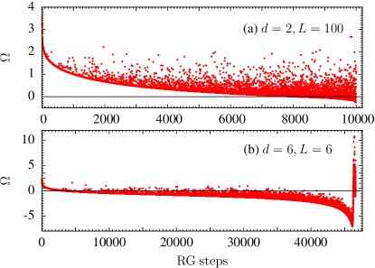
Figure 1: Representative evolution of $\Omega_{i}$ of the decimated spin as a function of the RG step, which corresponds to the number of spins which have been decimated for the EA model for (a) $d=2$ and (b) $d=6$. Over most of the iteration range for $d=2$, $\Omega_{i}$ is positive. The SDRG estimate for the exponent $d_{\rm s}$ is also quite accurate in this case. As $d$ increases, the values of $\Omega_{i}$ turn negative after a decreasing number of iterations, suggesting that the SDRG becomes less accurate in higher dimensions, as can be seen for $d=6$ [panel (b)]. Note the different horizontal scales.

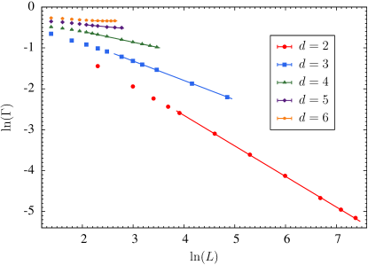
Figure 2: $\ln\Gamma$ for various space dimensions $d$ as a function of $\ln L$ computed using the SDRG algorithm. Note that $\Gamma\sim L^{d_{\rm s}-d}$. Our estimate of $d_{\rm s}$ is determined by the slope of the straight lines drawn through the points at large-$L$ values. Note how the data for $d=6$ level off, i.e., $d_{\rm s}\to d$. (See Fig. 3 for an enlarged figure in six dimensions). Error bars are smaller than the symbols.

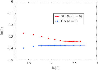
Figure 3: $\ln\Gamma$ for $d=6$ as a function of $\ln L$ computed using the SDRG and GA algorithms. Our estimate of $d_{\rm s}$ is determined by the slope of the straight lines drawn through the points at large-$L$ values. Using $\Gamma\sim L^{d_{\rm s}-d}$ the levelling off of the lines at the larger values of $L$ implies that $d_{\rm s}\to d$ in six dimensions. Error bars are smaller than the symbols.

Table 1: Dimensionality $d$, system size $L$, and the number of disorder realizations $M$ studied using the GA and SDRG methods. Part of the SDRG data used here are taken from Ref. Wang et al. (2017).

Method	$d$	$L$	$M$
SDRG	$2$	$\{10,20,30,40,50,100,200,400,800\}$	$10000$
SDRG	$2$	$1200$	$3000$
SDRG	$2$	$1600$	$1000$
SDRG	$3$	$\{4,6,8,10,12,16,20,24,32\}$	$3000$
SDRG	$3$	$\{64,128\}$	$1000$
SDRG	$4$	$\{4,5,6,7,8,9,10,12,16,20,24\}$	$3000$
SDRG	$4$	$28$	$717$
SDRG	$4$	$32$	$121$
SDRG	$5$	$\{4,5,6,7,8,9,10,12,14\}$	$3000$
SDRG	$5$	$16$	$1000$
SDRG	$6$	$\{4,5,6,7,8\}$	$3000$
SDRG	$6$	$9$	$1843$
SDRG	$6$	$10,11,12$	$1000$
SDRG	$6$	$\{13,14\}$	$200$
GA	$2$	$\{4,8,12,16,32,64,128,256,512\}$	$3000$
GA	$3$	$\{4,6,8,10,12,16,20,24,32,64\}$	$3000$
GA	$4$	$\{4,6,8,10,12,16,20,24,32\}$	$3000$
GA	$5$	$\{4,5,6,7,8,9,10\}$	$6000$
GA	$5$	$\{12,14,16\}$	$3000$
GA	$6$	$\{4,5,6,7,8,9,10\}$	$3000$
GA	$6$	$\{12,14\}$	$1000$

IV SDRG results

In Fig. 2 we plot $\ln\Gamma$ versus $\ln L$ using the SDRG method of Monthus Monthus (2015) to compute the link overlap. One change from our previous work in Ref. Wang et al. (2017) is that we have added more data. Especially for $d=6$ we have increased the largest system studied from $L=10$ to $L=14$. The new data show that for $d=6$ the curve is levelling off, implying that $d_{\rm s}\to d$. We have also increased the values of $L$ studied in $d=2$ and $3$, going far beyond the system sizes studied in Ref. Monthus (2015). Table 1 lists simulation parameters, such as the number of bond configurations $M$ for each value of the linear system size $L$ in space dimension $d$.

The SDRG seems to give quite accurate results for the value of $d_{\rm s}$ at least in low space dimensions. Thus, in $d=2$, Monthus found from the SDRG a value of $d_{\rm s}\approx 1.27$ from $L$ values up to $340$, a result which is similar to a recent study of systems up to $L=10^{4}$ Khoshbakht and Weigel (2018) based on fast polynomial time algorithms for finding ground states (which, however, only work in two space dimensions) which gives $d_{\rm s}=1.27319(9)$. In $d=3$, Monthus finds $d_{\rm s}=2.55$ for systems of size up to $L=45$. In Ref. Wang et al. (2017) a value of $2.57$ is quoted from studies on systems up to $L=12$. The SDRG is just an algorithm which attempts to find the ground-state spin configuration. It is exact in one space dimension. While it seems to give excellent values for $d_{\rm s}$, it gives poor values for the actual ground-state energy itself and the energy cost of the interface. If the domain-wall energy scales $\sim L^{\theta}$, then Monthus reports $\theta\approx 0$ whereas the recent high-precision calculations show that $\theta=-0.2793(3)$ Khoshbakht and Weigel (2018).

Because Monthus’ value for $d_{\rm s}$ in $d=2$ seemed to be compatible with the high-precision calculations Khoshbakht and Weigel (2018), we speculated in Ref. Wang et al. (2017) that the SDRG might be accurate because the interface is a self-similar fractal Mandelbrot (1967). The SDRG seems to be accurate in the early stages of the RG process where the $\Omega_{i}$ are positive (see Fig. 1) where a coarse approximation of the domain lengths is performed (see Fig. 4). In the later stages of determining the domain length, the SDRG’s accuracy will decrease. In particular, in the relation $\Sigma^{DW}\sim AL^{d_{\rm s}}$ we suspect that the SDRG might determine $d_{\rm s}$ quite accurately, but that the coefficient $A$ might be obtained with less accuracy. To estimate $A$ to high accuracy would require an RG process accurate on all length scales, both short and long. In this paper we have extended the system sizes studied far beyond those studied by Monthus in $d=2$, and find that $d_{\rm s}=1.2529(14)$ which indicates that the SDRG is not exact for $d_{\rm s}$ in $d=2$, but just a good approximation. Our estimate of $A$ is $1.4040(106)$ whereas the recent high-precision estimate is $1.222(3)$ Khoshbakht and Weigel (2018).

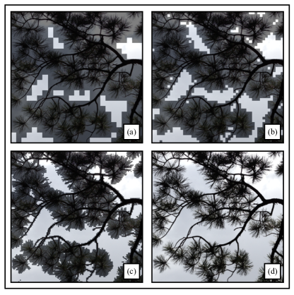
Figure 4: The bifurcation of a tree is a self-similar fractal. The four figures are measurements of its length using square domains whose linear size is reduced at each step of the renormalization. For a self-similar fractal, like the ponderosa pine depicted here, the scaling dimension $d_{\rm s}$ is the same no matter what length scale is used to determine it. Panel (a) shows the coarsest measurements which are successively refined by reducing the size of the squares in panels (b) – (d). Note that the domains are smaller than the image resolution in panel (d). The fractal dimension of the ponderosa pine is approximately $1.88$. One could in principle obtain the correct fractal dimension by studies at the coarsest length scales which is why we suspect that the SDRG, which works better on the coarsest length scales, is capable of getting accurate answers for $d_{\rm s}$.

We have also extended Monthus’ work in $d=3$ from $L=45$ to $L=128$ and find $d_{\rm s}=2.5256(30)$. If we had only system sizes up to $12$ in $d=3$, as in the Monte Carlo studies of Ref. Wang et al. (2017), then because of finite-size effects (visible in Fig. 2), we would have reported a value of $d_{\rm s}\approx 2.6093(50)$. A value of $2.57$ was reported in Ref. Wang et al. (2017) based on the same range of $L$ values up to $L=12$.

The SDRG is not an analytical treatment, but a numerical technique and in high dimensions (e.g., $d=5$ and $6$) this limits us to studying rather small linear system sizes. As a consequence, estimates of exponents can be affected by finite-size corrections as aforementioned for $d=3$. Thus, it is hard to be certain that $d_{\rm s}=d$ in six dimensions. We therefore decided to also use a greedy algorithm (GA) to complement the SDRG results. It is already known from analytical studies that $6$ is the ”upper critical dimension” for the GA, at least for the fractal dimension associated with minimum spanning trees. Jackson and Read (2010, 2010). Here, we want to know whether numerical studies of the value of $d_{\rm s}$ would also show that six is a similarly special dimension for the fractal dimension of domain walls with the GA algorithm.

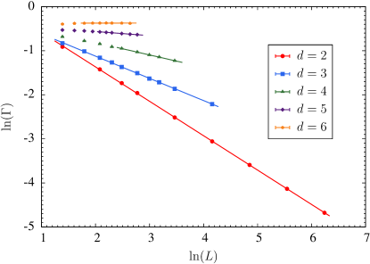
Figure 5: $\ln\Gamma$ for various space dimensions $d$ for the EA model as a function of $\ln L$ computed using the GA. Note that $\Gamma\sim L^{d_{\rm s}-d}$. Our estimate of $d_{\rm s}$ is determined by the slope of the straight lines drawn through the points at large $L$-values. Error bars are smaller than the symbols.

V The greedy algorithm

The GA (also studied by Monthus Monthus (2015)) works as follows. The bonds in the order of decreasing absolute magnitude are satisfied in turn, unless a closed loop appears then the bond is skipped, until the relative orientation of all the spins is determined. In Table 1, we have given details of the system sizes and numbers of different bond realizations which we have studied in dimensions $d=2$, $\cdots$, $6$. In Fig. 5 we plot $\ln\Gamma$ versus $\ln L$ determining the link overlap using the GA. Notice that the corrections to scaling in $d=6$ seem smaller for the GA than for the SDRG method, because the data seem independent of $L$ even for the smallest system sizes.

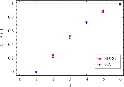
Figure 6: Greedy algorithm (GA) results (blue pentagons) compared with strong-disorder renormalization group (SDRG) results (red squares) for $d=2$, $3$, $4$, $5$, and $6$. The upper bound $d_{\rm s}-d+1$ at unity is marked by a horizontal blue line, while the lower bound at zero is marked with a horizontal red line. The value $d_{\rm s}=0$ for $d=1$ is exact and given by both methods. Only statistical errors are included and error bars are smaller than the symbols. Numerical values are summarized in Table. 2.

Like the SDRG procedure, the GA is just a way of finding the spin configuration for a putative ground state of the system. There is no bond renormalization as in the SDRG [see Eq. (11)]. It is just as poor for the ground-state energy and the exponent $\theta$ as the SDRG Monthus (2015). In $d=2$ we obtain $d_{\rm s}^{\rm GA}\simeq 1.2196(11)$, which is comparable with Ref. Sweeney and Middleton (2013) who quote $d_{\rm s}^{\rm GA}=1.216(1)$. Note that the SDRG value for $d_{\rm s}$ is in much better agreement with the high-precision value of Ref. Khoshbakht and Weigel (2018). In $d=3$ the GA result is $d_{\rm s}^{\rm GA}\simeq 2.4962(19)$, which is closer to that of the SDRG. An earlier estimate in three dimensions is that of Ref. Cieplak et al. (1994) who quote $d_{\rm s}^{\rm GA}\simeq 2.5\pm 0.05$. In Fig. 6 we have plotted $d_{\rm s}-d+1$ versus $d$ using the $d_{\rm s}$ from both the GA and SDRG algorithms. As the dimension $d$ approaches $6$ the two estimates appear to merge and give $d_{\rm s}=d$ in $d=6$. The analytical expectation of Refs. Jackson and Read (2010, 2010) was that $6$ is the upper critical dimension for the fractal dimension of minimum spanning trees within the GA. Our numerical work suggests that within the GA, domain walls also have $6$ as their upper critical dimension.

VI Discussion

Table 2: Numerical estimates of the fractal dimension $d_{s}$ of the SDRG and GA methods. $d_{s}$=0 for $d=1$, as both methods are exact for the one-dimensional model. Error bars are statistical errors.

Method	$d=2$	$d=3$	$d=4$	$d=5$	$d=6$
SDRG	1.2529(14)	2.5256(30)	3.7358(36)	4.884(60)	5.9899(60)
GA	1.2196(11)	2.4962(19)	3.7190(47)	4.9068(32)	6.0023(22)

We have obtained numerical results (Fig. 6) using a strong-disorder renormalization group method and a greedy algorithm that are consistent with $6$ being a special space dimension above which the conventional EA model with a Gaussian bond distribution has RSB behavior and summarized them in Table 2. For $d\leq 6$, we have found that within our numerical procedures that the EA model is behaving according to droplet model expectations because $d_{\rm s}<d$. That $6$ is a special dimension for the behavior of spin glasses is in accord with some older expectations based on analytical results Bray and Moore (1980); Moore and Bray (2011), but these have been controversial Parisi and Temesvári (2012); Moore and Read (2018). Because both the GA and the SDRG are approximations, we regard the results presented here as not decisive.

We note, however, that real-space RG methods such as the SDRG are capable of endless refinements. Monthus Monthus (2015) herself discussed a variant, the “box” method, which improved the value of the zero-temperature exponent $\theta$ in $d=2$ from the very poor value $\theta\approx 0$ obtained by the SDRG method described in this paper to at least a negative value of $\theta\approx-0.09$ [the high-precision estimate of Ref. Khoshbakht and Weigel (2018) is $\theta=-0.2793(3)$]; note that the value of $d_{\rm s}$ was hardly altered. It might be possible to find a real-space RG procedure that gives accurate numbers on all quantities of interest for three-dimensional spin glasses. The SDRG and the GA have a common feature in that they both recognize that the largest bonds are likely to be satisfied in the ground state. We suspect that will be an ingredient of any future successful RG scheme for spin-glass systems.