A viscosity-independent error estimate
of a pressure-stabilized Lagrange–Galerkin scheme
for the Oseen problem

Abstract

We consider a pressure-stabilized Lagrange–Galerkin scheme for the transient Oseen problem with small viscosity. In the scheme we use the equal-order approximation of order $k$ for both the velocity and pressure, and add a symmetric pressure stabilization term. We show an error estimate for the velocity with a constant independent of the viscosity if the exact solution is sufficiently smooth. Numerical examples show high accuracy of the scheme for problems with small viscosity.

Keywords:

Transient Oseen problem, Lagrange–Galerkin scheme, Finite element method, Equal-order elements, Symmetric pressure stabilization, Dependence on viscosity

1 Introduction

We consider a finite element scheme for the transient Oseen problem, known as linearizion of the Navier–Stokes problem, with small viscosity. In this paper we construct a pressure-stabilized Lagrange–Galerkin (LG) scheme with higher-order elements, and show an error estimate independent of the viscosity.

When the viscosity is small, the finite element method suffers from two kinds of instabilities. We begin with the issue of the material derivative. In such case the convection is dominated and it is important to put weight on information in the upwind direction to make schemes stable. We here focus on the LG method, e.g. [25, 26, 28, 31, 33], which is a combination of the characteristics method and the finite element method. One of the advantages of it is that the resultant matrix is symmetric, which allows us to use efficient linear solvers [3]. Recently a LG method with a locally linearized velocity [34] has been developed [33] and convergence has been shown. The locally linearized velocity overcomes the difficulty in computing composite function term that appears in LG schemes. In [33] inf-sup stable elements [6] were used.

Besides the inf-sup stable elements, $\mathrm{P}_{1}/\mathrm{P}_{1}$-element with a pressure stabilization term has been also used in LG methods, where $\mathrm{P}_{k}/\mathrm{P}_{l}$ shows that we use the conforming triangular or tetrahedral element of order $k$ for the velocity and order $l$ for the pressure. Notsu and Tabata have been proposed a LG scheme using the stabilization term of Brezzi and Pitkäranta [8] for the Navier–Stokes problem [23, 24], and analyzed the scheme for the Oseen problem and Navier–Stokes problem [25, 26]. Jia et al. [20] have been proposed and analyzed a LG scheme using the stabilization term of Bochev et al. [5].

Here we extend the $\mathrm{P}_{1}/\mathrm{P}_{1}$ pressure-stabilized LG scheme to higher-order elements. Simple symmetric stabilization terms for higher-order elements have been presented and applied to stationary problems in, e.g., [2, 7, 9, 14, 30] and to the transient Stokes problem in [10]. On the other hand, classical stabilization terms based on the residual of the momentum equations also have been studied for stationary problems in, e.g., [15, 16, 19] and for the transient Stokes problem in [22]. These terms are, however, rather complicated to implement compared to the symmetric stabilization especially for transient problems.

Apart from the issue of the material derivative in the Oseen or Navier–Stokes problems, dependence on the viscosity appears even in the Stokes problems. Numerical solutions of the velocities contain approximation errors of the pressures multiplied by the inverse of the viscosity in standard finite element methods (e.g. [21]). The grad-div stabilization [17] is a choice to improve stability. Error analyses independent of the viscosity were performed in [27] for the Stokes problem and in [13] for the transient Oseen problem relying on this term. In [4] a LG scheme was developed for the Navier–Stokes problem with local projection stabilization that includes the grad-div term.

In this paper we use $\mathrm{P}_{k}/\mathrm{P}_{k}$-element, $k\geq 1$, and pressure-stabilization in the LG scheme for the transient Oseen problem, and show an error estimate independent of the viscosity. In the scheme the symmetric pressure stabilization of Burman [9] is used and symmetry of the LG method is inherited. Although a pressure stabilized scheme for the transient Stokes problem has been analyzed by Burman and Fernández [10], we here pay attention to the constant of the stabilization term. We consider the case where the viscosity $\nu$ is small and the exact solution is sufficiently smooth. The error bound presented here is of order $\Delta t+h^{2}+h^{k}$ in the $L^{2}$-norm for the velocity and for $\nu^{1/2}$ times the gradient of the velocity, with constants independent of $\nu$. Here, $\Delta t$ is a time increment, $h$ is a spacial mesh size. This scheme is essentially unconditionally stable, that is, we can take $\Delta t$ and $h$ independently. The grad-div stabilization is not needed in our analysis. The technique used in our estimate is a projection of the exact solution of the velocity with the error independent of $\nu$. A similar way was used by de Frutos et al. [13].

This paper is organized as follows. In the next section, after preparing notation, we state the Oseen problem and a pressure-stabilized LG scheme. In Section 3 we show an error estimate with a constant independent of the viscosity and give a proof. In Section 4 we give some numerical results that show high accuracy for small viscosity and large pressures, and additionally show results of the Navier–Stokes problem. In Section 5 we give conclusions. In Appendix we recall some lemmas used in the LG methods.

2 A pressure-stabilized LG scheme for the Oseen problem

We prepare notation used throughout this paper, state the Oseen problem and then introduce our scheme.

Let $\Omega$ be a polygonal or polyhedral domain of $\mathbb{R}^{d}~{}(d=2,3)$. We use the Sobolev spaces $W^{m,p}(\Omega)$ equipped with the norm $\|\cdot\|_{m,p}$ and the semi-norm $|\cdot|_{m,p}$ for $p\in[1,\infty]$ and a non-negative integer $m$. We denote $W^{0,p}(\Omega)$ by $L^{p}(\Omega)$. $W^{1,p}_{0}(\Omega)$ is the subspace of $W^{1,p}(\Omega)$ consisting of functions whose traces vanish on the boundary of $\Omega$. When $p=2$, we denote $W^{m,2}(\Omega)$ by $H^{m}(\Omega)$ and drop the subscript $2$ in the corresponding norm and semi-norm. For the vector-valued function $w\in W^{1,\infty}(\Omega)^{d}$ we define the semi-norm $|w|_{1,\infty}$ by

$$\biggl{\lVert}\biggl{[}\sum_{i,j=1}^{d}\left(\frac{\partial w_{i}}{\partial x_{j}}\right)^{2}\biggr{]}^{1/2}\biggr{\rVert}_{0,\infty}.$$

The pair of parentheses $(\cdot,\cdot)$ shows the $L^{2}(\Omega)^{i}$-inner product for $i=1,d$ or $d\times d$. $L^{2}_{0}(\Omega)$ is the space of functions $q\in L^{2}(\Omega)$ satisfying $(q,1)=0$. We also use the notation $|\cdot|_{m,K}$ and $(\cdot,\cdot)_{K}$ for the semi-norm and the inner product on a set $K$.

Let $T>0$ be a time. For a Sobolev space $X(\Omega)^{i}$, $i=1,d$, we use the abbreviations $H^{m}(X)=H^{m}(0,T;X(\Omega)^{i})$ and $C(X)=C([0,T];X(\Omega)^{i})$. We define the function space $Z^{m}$ by

$$\begin{split}Z^{m}&:=\{v\in H^{j}(0,T;H^{m-j}(\Omega)^{d});~{}j=0,\dots,m,\|v\|_{Z^{m}}<\infty\},\\ \|v\|_{Z^{m}}&:=\biggl{(}\sum_{j=0}^{m}\|v\|_{H^{j}(0,T;H^{m-j}(\Omega)^{d})}^{2}\biggr{)}^{1/2}.\end{split}$$

We also use the notation $H^{m}(t_{1},t_{2};X)$ and $Z^{m}(t_{1},t_{2})$ for spaces on a time interval $(t_{1},t_{2})$.

We consider the Oseen problem: find $(u,p):\Omega\times(0,T)\to\mathbb{R}^{d}\times\mathbb{R}$ such that

$$\begin{split}\frac{\partial u}{\partial t}+(w\cdot\nabla)u-\nu\Delta u+\nabla p=f&\quad\text{in}\quad\Omega\times(0,T),\\ \nabla\cdot u=0&\quad\text{in}\quad\Omega\times(0,T),\\ u=0&\quad\text{on}\quad\partial\Omega\times(0,T),\\ u(\cdot,0)=u^{0}&\quad\text{in}\quad\Omega,\end{split}$$ (1)

where $\partial\Omega$ represents the boundary of $\Omega$, the constant $0<\nu\leq 1$ represents a viscosity, and $w,f:\Omega\times(0,T)\to\mathbb{R}^{d}$ and $u^{0}:\Omega\to\mathbb{R}^{d}$ are given functions.

We define the bilinear forms $a$ on $H^{1}_{0}(\Omega)^{d}\times H^{1}_{0}(\Omega)^{d}$ and $b$ on $H^{1}_{0}(\Omega)^{d}\times L^{2}_{0}(\Omega)$ by

$$a(u,v):=\nu(\nabla u,\nabla v),\quad b(v,q):=-(\nabla\cdot v,q).$$

Then, we can write the weak form of (1) as follows: find $(u,p):(0,T)\to H^{1}_{0}(\Omega)^{d}\times L^{2}_{0}(\Omega)$ such that for $t\in(0,T)$,

$$\left(\Bigl{(}\frac{\partial u}{\partial t}+(w\cdot\nabla)u\Bigr{)}(t),v\right)+a(u(t),v)+b(v,p(t)) =(f(t),v),$$ (2a)

$$\forall v\in H^{1}_{0}(\Omega)^{d},$$

$$b(u(t),q)=0,\quad \forall q\in L^{2}_{0}(\Omega),$$ (2b)

with $u(0)=u^{0}$.

We introduce time discretization. Let $\Delta t>0$ be a time increment, $N_{T}:=\lfloor T/\Delta t\rfloor$ the number of time steps, $t^{n}:=n\Delta t$, and $\psi^{n}:=\psi(\cdot,t^{n})$ for a function $\psi$ defined in $\Omega\times(0,T)$. For a set of functions $\psi=\{\psi^{n}\}_{n=0}^{N_{T}}$ we use two norms $\|\cdot\|_{\ell^{\infty}(L^{2})}$ and $\|\cdot\|_{\ell^{2}(L^{2})}$ defined by

$$\begin{split}\|\psi\|_{\ell^{\infty}(L^{2})}&:=\max\left\{\|\psi^{n}\|_{0};n=0,\dots,N_{T}\right\},\\ \|\psi\|_{\ell^{2}(L^{2})}&:=\biggl{(}\Delta t\sum_{n=1}^{N_{T}}\|\psi^{n}\|_{0}^{2}\biggr{)}^{1/2}.\end{split}$$

Let $w$ be smooth. The characteristic curve $X(t;x,s)$ is defined by the solution of the system of the ordinary differential equations,

$$\begin{split}\frac{dX}{dt}(t;x,s)&=w(X(t;x,s),t),\quad t<s,\\ X(s;x,s)&=x.\end{split}$$ (3)

Then, we can write the material derivative term $\frac{\partial u}{\partial t}+(w\cdot\nabla)u$ as follows:

$$\left(\frac{\partial u}{\partial t}+(w\cdot\nabla)u\right)(X(t),t)=\frac{d}{dt}u(X(t),t).$$

For $w^{*}:\Omega\to\mathbb{R}^{d}$ we define the mapping $X_{1}(w^{*}):\Omega\to\mathbb{R}^{d}$ by

$$(X_{1}(w^{*}))(x):=x-w^{*}(x)\Delta t.$$ (4)

Remark 1.

The image of $x$ by $X_{1}(w(\cdot,t))$ is nothing but the approximate value of $X(t-\Delta t;x,t)$ obtained by solving (3) by the backward Euler method.

Then, it holds that

$$\frac{\partial u^{n}}{\partial t}+(w^{n}\cdot\nabla)u^{n}=\frac{u^{n}-u^{n-1}\circ X_{1}(w^{n-1})}{\Delta t}+O(\Delta t),$$

where the symbol $\circ$ stands for the composition of functions, e.g., $(g\circ f)(x):=g(f(x))$.

We next introduce spacial discretization. Let $\{\mathcal{T}_{h}\}_{h\downarrow 0}$ be a regular family of triangulations of $\overline{\Omega}$ [11], $h_{K}:=\operatorname{diam}(K)$ for an element $K\in\mathcal{T}_{h}$, and $h:=\max_{K\in\mathcal{T}_{h}}h_{K}$. For a positive integer $m$, the finite element space of order $m$ is defined by

$$W_{h}^{(m)}:=\{\psi_{h}\in C(\overline{\Omega});~{}\psi_{h|K}\in\mathrm{P}_{m}(K),~{}\forall K\in\mathcal{T}_{h}\},$$

where $\mathrm{P}_{m}(K)$ is the set of polynomials on $K$ whose degrees are equal to or less than $m$. Let $\Pi_{h}^{(m)}:C(\overline{\Omega})\to W_{h}^{(m)}$ be the Lagrange interpolation operator, which is naturally extended to vector-valued functions.

We begin with a scheme using the standard $\mathrm{P}_{k}/\mathrm{P}_{k-1}$-finite element, which is called (generalized) Taylor–Hood element. Let

$$V_{h}\times\overline{Q}_{h}:=((W_{h}^{(k)})^{d}\cap H_{0}^{1}(\Omega)^{d})\times(W_{h}^{(k-1)}\cap L_{0}^{2}(\Omega))$$ (5)

be the $\mathrm{P}_{k}/\mathrm{P}_{k-1}$-finite element space for $k\geq 2$. The LG scheme with a locally linearized velocity and this Taylor–Hood element for the Oseen problem (OsTH) is stated as follows:

Scheme OsTH.

Let $u_{h}^{0}\in V_{h}$ be an approximation of $u^{0}$. Find $\{(u_{h}^{n},p_{h}^{n})\}_{n=1}^{N_{T}}\subset V_{h}\times\overline{Q}_{h}$ such that

$$\biggl{(}\frac{u_{h}^{n}-u_{h}^{n-1}\circ X_{1}(\Pi_{h}^{(1)}w^{n-1})}{\Delta t},v_{h}\biggr{)}+a(u_{h}^{n},v_{h})+ b(v_{h},p_{h}^{n})\qquad$$

$$=(f^{n},v_{h}),~{} \forall v_{h}\in V_{h},$$ (6a)

$$b(u_{h}^{n},q_{h}) =0,~{} \forall q_{h}\in\overline{Q}_{h},$$ (6b)

When $k=2$, this type of scheme for the Navier–Stokes problem has already been introduced and analyzed in [33]. In the mapping $X_{1}(\cdot)$, a locally linearized velocity $\Pi_{h}^{(1)}w^{n-1}$ is used instead of the original velocity $w^{n-1}$. If the original velocity is used, it is difficult to evaluate the exact value of integration. The next proposition assures that the scheme with the locally linearized velocity is exactly computable.

Proposition ([32, 33]).

Let $u_{h}$, $v_{h}\in(W_{h}^{(m)})^{d}$ for a positive integer $m$. Suppose that

$$w^{*}\in W^{1,\infty}_{0}(\Omega)^{d}\quad\text{and}\quad\alpha_{*}\Delta t|w^{*}|_{1,\infty}<1,$$ (7)

where $\alpha_{*}$ is the constant defined in (11) below. Then, $\int_{\Omega}(u_{h}\circ X_{1}(\Pi_{h}^{(1)}w^{*}))\cdot v_{h}dx$ is exactly computable.

With the assumption (7) for $w^{*}=w^{n-1}$ at each step $n$, (6) is exactly computable thanks to Proposition. In [33] the authors have analyzed the scheme to show the estimates

$$\|\nabla(u_{h}-u)\|_{\ell^{\infty}(L^{2})},~{}\|p_{h}-p\|_{\ell^{2}(L^{2})}\leq c(\nu^{-1})(\Delta t+h^{2}),$$

where the constant $c$ depends on $\nu^{-1}$ exponentially.

Here we use the equal-order element with pressure stabilization. Let

$$V_{h}\times Q_{h}:=((W_{h}^{(k)})^{d}\cap H_{0}^{1}(\Omega)^{d})\times(W_{h}^{(k)}\cap L_{0}^{2}(\Omega))$$

be the equal-order $\mathrm{P}_{k}/\mathrm{P}_{k}$-finite element space for $k\geq 1$. We define a pressure stabilization term $\mathcal{C}_{h}:Q_{h}\times Q_{h}\to\mathbb{R}$, which enables us to use the equal-order element, by

$$\begin{split}\mathcal{C}_{h}(p_{h},q_{h}):=\sum_{K\in\mathcal{T}_{h}}h_{K}^{2k}\sum_{|\alpha|=k}(D^{\alpha}p_{h},D^{\alpha}q_{h})_{K},\end{split}$$

where $\alpha$ is the multi-index and $D^{\alpha}$ is the partial differential operator. We define the corresponding semi-norm on $Q_{h}$ by

$$|q_{h}|_{h}:=\mathcal{C}_{h}(q_{h},q_{h})^{1/2}=\left(\sum_{K\in\mathcal{T}_{h}}h_{K}^{2k}|q_{h}|_{k,K}^{2}\right)^{1/2}.$$ (8)

Remark 2.

The term $\mathcal{C}_{h}$ introduced by Burman [9] is an extension of that by Brezzi and Pitkäranta [8] for the $\mathrm{P}_{1}/\mathrm{P}_{1}$-element to higher order elements. For the stabilization term, instead of $\mathcal{C}_{h}$, we can also choose another positive semi-definite bilinear form whose corresponding semi-norm is equivalent to (8). Examples include the terms in [2, 14, 30], as pointed out in [9].

We are now in position to state a pressure-stabilized LG scheme for the Oseen problem (OsPstab).

Scheme OsPstab.

Let $u_{h}^{0}\in V_{h}$ be an approximation of $u^{0}$. Find $\{(u_{h}^{n},p_{h}^{n})\}_{n=1}^{N_{T}}\subset V_{h}\times Q_{h}$ such that

$$\biggl{(}\frac{u_{h}^{n}-u_{h}^{n-1}\circ X_{1}(\Pi_{h}^{(1)}w^{n-1})}{\Delta t},v_{h}\biggr{)}+a(u_{h}^{n},v_{h})+b(v_{h},p_{h}^{n})\qquad$$

$$=(f^{n},v_{h}),~{}\forall v_{h}\in V_{h},$$ (9a)

$$b(u_{h}^{n},q_{h})-\delta_{0}\mathcal{C}_{h}(p_{h}^{n},q_{h})=0,~{}\forall q_{h}\in Q_{h},$$ (9b)

where $\delta_{0}>0$ is a stabilization parameter.

With the assumption (7) for $w^{*}=w^{n-1}$ at each step $n$, (9) is exactly computable and has a unique solution $(u_{h}^{n},p_{h}^{n})$ thanks to Proposition and the stabilization term $\mathcal{C}_{h}$ [9]. The error introduce by the locally linearized velocity is properly estimated in Theorem below.

Remark 3.

1. In Scheme OsPstab, the resultant matrix to be solved is symmetric, which enables us to use efficient linear solvers [3].

2. When $k=1$, Notsu and Tabata [25] proposed and analyzed a pressure-stabilized LG scheme, where the locally linearized velocity was not introduced.

3. Burman and Fernández [10] proposed and analyzed a scheme for the transient Stokes problem using a same type of pressure stabilization. Since in their choice the stabilization parameter $\delta_{0}$ is proportional to $1/\nu$, it seems to be difficult to get error estimates independent of $\nu$, which we will show in the next section.

3 An error estimate focused on the viscosity for the Oseen problem

Before stating the result we introduce hypotheses.

Hypothesis 1.

The velocity $w$ and the exact solution $(u,p)$ of the Oseen problem (1) satisfies

$$w\in C(W^{1,\infty}_{0}\cap W^{2,\infty})\cap H^{1}(L^{\infty}),~{}u\in Z^{2}\cap H^{1}(H^{k+1}),~{}p\in C(H^{k+1}).$$

Hypothesis 2.

The time increment $\Delta t$ satisfies $0<\Delta t\leq\Delta t_{0}$, where

$$\Delta t_{0}:=\frac{1}{4\alpha_{*}|w|_{C(W^{1,\infty})}},$$

and $\alpha_{*}$ is the constant defined in (11) below.

Hypothesis 3 (Triangulation).

Every element $K\in\mathcal{T}_{h}$ has at least one internal vertex.

Hypothesis 4 (Choice of the initial value).

There exists a positive constant $c$ independent of $h$ such that

$$\|u_{h}^{0}-u^{0}\|_{0}\leq ch^{k}|u^{0}|_{k}.$$

Remark 4.

1. Hypothesis 1 implies that $u\in C(H^{k+1})$ and $u^{0}\in H^{k+1}(\Omega)^{d}$.

2. Under Hypotheses 1 and 2, the property (7) for $w^{*}=w^{n-1}$ at each step $n$ is clearly satisfied.

3. Hypothesis 4 is satisfied if we take $u_{h}^{0}$ as the Lagrange interpolation of $u^{0}$, for example.

Theorem.

Let $V_{h}\times Q_{h}$ be the $\mathrm{P}_{k}/\mathrm{P}_{k}$-finite element space for $k\geq 1$. Suppose Hypotheses 1–4. Let $(u_{h},p_{h}):=\{(u_{h}^{n},p_{h}^{n})\}_{n=0}^{N_{T}}$ be the solution of Scheme OsPstab. Then there exists a positive constant $c_{*}$ independent of $\nu$, $h$, $\Delta t$ such that

$$\|u_{h}-u\|_{\ell^{\infty}(L^{2})},\sqrt{\nu}\|\nabla(u_{h}-u)\|_{\ell^{2}(L^{2})}\leq c_{*}(\Delta t+h^{2}+h^{k}).$$ (10)

Remark 5.

1. The constant $c_{*}$ depends on Sobolev norms of $w,u$ and $p$, and the stabilization parameter $\delta_{0}$. Note also that we assumed that $\nu\leq 1$. The parameter $\delta_{0}$ should not depend on $\nu$ from the viewpoint of this estimate.

2. If $\mathrm{P}_{k}/\mathrm{P}_{k-1}$-element is employed, we have an estimate of the same order $\Delta t+h^{2}+h^{k}$, but it seems to be difficult to remove the dependence on the viscosity, which is observed in the numerical experiments in Section 4.

3. The term $h^{2}$ appears in (10) because of the introduction of the locally linearized velocity.

4. It seems to be difficult to derive the estimate $h^{k+1}$ for the spacial discretization in $\ell^{\infty}(L^{2})$ independent of the viscosity. Although another type of Stokes projection yields an estimate of order $h^{k+1}$, e.g. [25], the projection error contains the dependence. de Frutos et al. [13] derived the same order $h^{k}$ as ours independent of the viscosity for the backward Euler method or the BDF2 formula with the grad-div stabilization.

5. Here we do not discuss a estimate for the pressure. de Frutos et al. [13] used inf-sup stable elements and show an estimate for the pressure independent of the viscosity. However, further discussion seems to be necessary for the pressure-stabilized method.

6. When $k=1$, Notsu and Tabata [25] analyzed the pressure-stabilized LG scheme without the locally linearized velocity. They derived the estimates

   $$\|\nabla(u_{h}-u)\|_{\ell^{\infty}(L^{2})},~{}\|p_{h}-p\|_{\ell^{2}(L^{2})}\leq c(\nu^{-1})(\Delta t+h),$$

   where the constant $c$ depends on $\nu^{-1}$ exponentially.

Before the proof we prepare some lemmas. First we recall a discrete version of the Gronwall inequality.

Lemma 1 (discrete Gronwall inequality).

Let $a_{0}$ and $a_{1}$ be non-negative numbers, $\Delta t\in(0,\frac{1}{2a_{0}}]$ be a real number, and $\{x^{n}\}_{n\geq 0},\{y^{n}\}_{n\geq 1}$ and $\{b^{n}\}_{n\geq 1}$ be non-negative sequences. Suppose

$$\frac{x^{n}-x^{n-1}}{\Delta t}+y^{n}\leq a_{0}x^{n}+a_{1}x^{n-1}+b^{n},~{}\forall n\geq 1.$$

Then, it holds that

$$x^{n}+\Delta t\sum_{i=1}^{n}y^{i}\leq\exp[(2a_{0}+a_{1})n\Delta t]\left(x^{0}+\Delta t\sum_{i=1}^{n}b^{i}\right),~{}\forall n\geq 1.$$

Lemma 1 is shown by using the inequalities

$$\frac{1}{1-a_{0}\Delta t}\leq 1+2a_{0}\Delta t\leq\exp(2a_{0}\Delta t).$$

In Lemmas 2–4 below, the constants $c$ are independent of $h$.

We recall the fundamental properties of Lagrange and Clément interpolations [11, 12].

Lemma 2.

Suppose that $\{\mathcal{T}_{h}\}_{h\downarrow 0}$ is a regular family of triangulations of $\overline{\Omega}$.
(i) Let $\Pi_{h}^{(m)}:C(\overline{\Omega})^{i}\to(W_{h}^{(m)})^{i}$, $i=1,d$, be the Lagrange interpolation operator to $\mathrm{P}_{m}$-finite element space for a positive integer $m$. Then there exist positive constants $\alpha_{*}\geq 1$ and $c$ independent of $h$ such that

$$|\Pi_{h}^{(1)}w|_{1,\infty} \leq\alpha_{*}|w|_{1,\infty},\quad\forall w\in W^{1,\infty}(\Omega)^{d},$$ (11)

$$\|\Pi_{h}^{(1)}w-w\|_{0,\infty} \leq ch^{2}|w|_{2,\infty},~{}\forall w\in W^{2,\infty}(\Omega)^{d},$$

$$\|\Pi_{h}^{(m)}w-w\|_{0,K} \leq ch_{K}^{m+1}|w|_{m+1,K},~{}\forall K\in\mathcal{T}_{h},\forall w\in H^{m+1}(K)^{i},i=1,d.$$

(ii) Let $\Pi_{h,C}^{(m)}:L^{2}(\Omega)\to W_{h}^{(m)}$ be the Clément interpolation operator to $\mathrm{P}_{m}$-finite element space for a positive integer $m$. Then there exists a positive constants $c$ such that

$$|\Pi_{h,C}^{(m)}\psi-\psi|_{1} \leq ch^{m}|\psi|_{m+1}, ~{}\forall\psi\in H^{m+1}(\Omega),$$

$$\biggl{(}\sum_{K\in\mathcal{T}_{h}}|\Pi_{h,C}^{(m)}\psi|_{m,K}^{2}\biggr{)}^{1/2} \leq c|\psi|_{m}, ~{}\forall\psi\in H^{m}(\Omega).$$

When $k\geq 2$, we use the auxiliary $\mathrm{P}_{k-1}$-pressure space $\overline{Q}_{h}$ defined in (5), and $(\widehat{z}_{h},\widehat{r}_{h})\in V_{h}\times\overline{Q}_{h}$ be the Stokes projection of $(z,r)\in H^{1}_{0}(\Omega)^{d}\times L^{2}_{0}(\Omega)$ for the fixed viscosity $\nu=1$ defined by

$$(\nabla\widehat{z}_{h},\nabla v_{h})-(\nabla\cdot v_{h},\widehat{r}_{h}) =(\nabla z,\nabla v_{h})-(\nabla\cdot v_{h},r),\quad \forall v_{h}\in V_{h},$$ (12a)

$$-(\nabla\cdot\widehat{z}_{h},\overline{q}_{h}) =-(\nabla\cdot z,\overline{q}_{h}), \forall\overline{q}_{h}\in\overline{Q}_{h}.$$ (12b)

Lemma 3.

Suppose that $\{\mathcal{T}_{h}\}_{h\downarrow 0}$ is a regular family of triangulations of $\overline{\Omega}$ and Hypothesis 3. Let $V_{h}\times\overline{Q}_{h}$ be the $\mathrm{P}_{k}/\mathrm{P}_{k-1}$-finite element space for $k\geq 2$. Then, there exists a positive constant $c$ such that

$$\|\widehat{z}_{h}-z\|_{1},\|\widehat{r}_{h}-r\|_{0}\leq ch^{k}(|z|_{k+1}+|r|_{k}),$$ (13)

where $(\widehat{z}_{h},\widehat{r}_{h})\in V_{h}\times\overline{Q}_{h}$ is the Stokes projection of $(z,r)\in(H^{1}_{0}(\Omega)^{d}\cap H^{k+1}(\Omega)^{d})\times(L^{2}_{0}(\Omega)\cap H^{k}(\Omega))$ defined in (12).

This estimate is a direct consequence of the inf-sup stability for the $\mathrm{P}_{k}/\mathrm{P}_{k-1}$-element [6]. Since in (12) the fixed viscosity is used, we have the estimate of the projection independent of the viscosity.

Lemma 4.

Suppose that $z\in H^{k+1}(\Omega)^{d}$ satisfies $\nabla\cdot z=0$, $\{\mathcal{T}_{h}\}_{h\downarrow 0}$ is a regular family of triangulations of $\overline{\Omega}$ and Hypothesis 3. Let $V_{h}\times Q_{h}$ be the $\mathrm{P}_{k}/\mathrm{P}_{k}$-finite element space for $k\geq 1$. Let $z_{h}\in V_{h}$ be the Lagrange interpolation of $z$ when $k=1$, or the first component of the Stokes projection of $(z,0)$ defined in (12) when $k\geq 2$. Then, there exists a positive constant $c$ such that

$$b(z_{h},q_{h})\leq ch^{k}|z|_{k+1}|q_{h}|_{h},~{}\forall q_{h}\in Q_{h},$$ (14)

where the semi-norm $|\cdot|_{h}$ is defined in (8)

Proof.

When $k=1$, by using $\nabla\cdot z=0$, the integration by part and Lemma 2, we get the estimate (14) as follows:

$$\begin{split}b(z_{h},q_{h})&=b(z_{h}-z,q_{h})=(z_{h}-z,\nabla q_{h})\leq c\sum_{K\in\mathcal{T}_{h}}h_{K}^{2}|z|_{2,K}\|\nabla q_{h}\|_{0,K}\\ &\leq ch|z|_{2}|q_{h}|_{h}.\end{split}$$

When $k\geq 2$, it holds that from (12b) and Lemma 2

$$b(z_{h},\overline{q}_{h})=b(z,\overline{q}_{h})=0,~{}\forall\overline{q}_{h}\in\overline{Q}_{h},\text{ and }$$

$$\|q_{h}-\overline{\Pi}_{h}^{(k-1)}q_{h}\|_{0}\leq\|q_{h}-\Pi_{h}^{(k-1)}q_{h}\|_{0}\leq c\left(\sum_{K\in\mathcal{T}_{h}}h_{K}^{2k}|q_{h}|_{k,K}^{2}\right)^{1/2},$$

where $\overline{\Pi}_{h}^{(k-1)}q_{h}\in\overline{Q}_{h}$ is the Lagrange interpolation of $q_{h}$ with the correction of the constant so that $\overline{\Pi}_{h}^{(k-1)}q_{h}\in L^{2}_{0}(\Omega)$. By Lemma 3 we get the estimate (14) as follows:

$$\begin{split}&b(z_{h},q_{h})=b(z_{h},q_{h}-\overline{\Pi}_{h}^{(k-1)}q_{h})\\ \leq&\|\nabla\cdot(z_{h}-z)\|_{0}\|q_{h}-\overline{\Pi}_{h}^{(k-1)}q_{h}\|_{0}\leq ch^{k}|z|_{k+1}|q_{h}|_{h}.\end{split}$$

∎

We now begin the proof of Theorem, where we also refer to Lemmas 6–9 in Appendix for properties of the mapping $X_{1}(\cdot)$.

Proof of Theorem.

Here we simply write $X_{1h}^{n-1}=X_{1}(\Pi_{h}^{(1)}w^{n-1})$. We use $c$ to represent a generic positive constant that is independent of $\nu$, $\Delta t$ and $h$ but depends on Sobolev norms $\|u\|_{C(H^{1})}$ and $\|w\|_{C(W^{2,\infty})}$, and may take a different value at each occurrence.

Let $z_{h}(t)\in V_{h}$ be, as in Lemma 4, the Lagrange interpolation of $u(t)$ when $k=1$, or the first component of the Stokes projection of $(u(t),0)$ defined in (12) when $k\geq 2$, and let $r_{h}(t)\in Q_{h}$ be the Clément interpolation of $p(t)$ with the correction of the constant so that $r_{h}(t)\in L^{2}_{0}(\Omega)$. We define the error terms by

$$(e_{h}^{n},\varepsilon_{h}^{n}):=(u_{h}^{n}-z_{h}^{n},p_{h}^{n}-r_{h}^{n}),~{}\eta(t):=u(t)-z_{h}(t).$$

From (9a), (2a) with $t=t^{n}$ and $v=v_{h}$, and (9b), we have an error equations in $(e_{h}^{n},\varepsilon_{h}^{n})$:

$$\left(\frac{e_{h}^{n}-e_{h}^{n-1}\circ X_{1h}^{n-1}}{\Delta t},v_{h}\right)+a(e_{h}^{n},v_{h})+b(v_{h},\varepsilon_{h}^{n})$$

$$=(R^{n},v_{h})+a(\eta^{n},v_{h})+b(v_{h},p^{n}-r_{h}^{n}), \forall v_{h}\in V_{h},$$ (15a)

$$b(e_{h}^{n},q_{h})-\delta_{0}\mathcal{C}_{h}(\varepsilon_{h}^{n},q_{h})=-b(z_{h}^{n},q_{h})+\delta_{0}\mathcal{C}_{h}(r_{h}^{n},q_{h}), \forall q_{h}\in Q_{h},$$ (15b)

for $n=1,\dots,N_{T}$, where $R^{n}:=R^{n}_{1}+R^{n}_{2}+R^{n}_{3}$,

$$\begin{split}R_{1}^{n}&:=\frac{\partial u^{n}}{\partial t}+(w^{n}\cdot\nabla)u^{n}-\frac{u^{n}-u^{n-1}\circ X_{1}(w^{n-1})}{\Delta t},\\ R_{2}^{n}&:=\frac{u^{n-1}\circ X_{1h}^{n-1}-u^{n-1}\circ X_{1}(w^{n-1})}{\Delta t},\\ R_{3}^{n}&:=\frac{\eta^{n}-\eta^{n-1}\circ X_{1h}^{n-1}}{\Delta t}.\end{split}$$ (16)

Substituting $(v_{h},q_{h})=(e_{h}^{n},\varepsilon_{h}^{n})$ in (15) and using the identity $(a-b)a=1/2(a^{2}-b^{2}+(a-b)^{2})$ yields

$$\begin{split}&\frac{1}{2\Delta t}\bigl{(}\|e_{h}^{n}\|_{0}^{2}-\|e_{h}^{n-1}\circ X_{1h}^{n-1})\|_{0}^{2}+\|e_{h}^{n}-e_{h}^{n-1}\circ X_{1h}^{n-1}\|_{0}^{2}\bigr{)}+\nu\|\nabla e_{h}^{n}\|_{0}^{2}+\delta_{0}|\varepsilon_{h}^{n}|_{h}^{2}\\ &=(R^{n},e_{h}^{n})+a(\eta^{n},e_{h}^{n})+b(e_{h}^{n},p^{n}-r_{h}^{n})+b(z_{h}^{n},\varepsilon_{h}^{n})-\delta_{0}\mathcal{C}_{h}(r_{h}^{n},\varepsilon_{h}^{n}).\end{split}$$ (17)

We now estimate the terms in (17). With Hypothesis 2 and the properties

$$\Pi_{h}^{(1)}w^{n-1}\in W^{1,\infty}_{0}(\Omega)^{d}\quad\text{and}\quad|\Pi_{h}^{(1)}w^{n-1}|_{1,\infty}\Delta t\leq\alpha_{*}|w^{n-1}|_{1,\infty}\Delta t\leq 1/4,$$ (18)

we use Lemma 6 in Appendix to have

$$\|e_{h}^{n-1}\circ X_{1h}^{n-1}\|_{0}^{2}\leq(1+c\Delta t)\|e_{h}^{n-1}\|_{0}^{2}.$$ (19)

After applying Schwarz’s inequality to $(R^{n},e_{h}^{n})$, we estimate $\|R_{i}^{n}\|_{0}$, $i=1,2,3$. By Lemma 7 in Appendix,

$$\|R_{1}^{n}\|_{0}\leq c\sqrt{\Delta t}\biggl{(}\|u\|_{Z^{2}(t^{n-1},t^{n})}+\left\|\frac{\partial w}{\partial t}\right\|_{L^{2}(t^{n-1},t^{n};L^{\infty})}\biggr{)}.$$ (20)

By Lemma 8 in Appendix with $q=2$, $p=\infty$, $p^{\prime}=1$, $w_{1}=\Pi_{h}^{(1)}w^{n-1}$, $w_{2}=w^{n-1}$ and $v=u^{n-1}$, and by Lemma 2,

$$\|R_{2}^{n}\|_{0}\leq c\|\Pi_{h}^{(1)}w^{n-1}-w^{n-1}\|_{0,\infty}\leq ch^{2}.$$ (21)

By Lemma 9 in Appendix with $v=\eta$ and $w^{*}=\Pi_{h}^{(1)}w^{n-1}$, and by Lemma 2 or 3,

$$\begin{split}\|R_{3}^{n}\|_{0}&\leq\frac{c}{\sqrt{\Delta t}}\biggl{(}\left\|\frac{\partial\eta}{\partial t}\right\|_{L^{2}(t^{n-1},t^{n};L^{2})}+\|\nabla\eta\|_{L^{2}(t^{n-1},t^{n};L^{2})}\biggr{)}\\ &\leq\frac{ch^{k}}{\sqrt{\Delta t}}\biggl{(}\|u\|_{H^{1}(t^{n-1},t^{n};H^{k+1})}\biggr{)}.\end{split}$$ (22)

An estimate for $a$ is easily obtained by Lemma 2 or 3:

$$a(\eta^{n},e_{h}^{n})\leq\frac{\nu}{2}\|\nabla\eta^{n}\|_{0}^{2}+\frac{\nu}{2}\|\nabla e_{h}^{n}\|_{0}^{2}\leq ch^{2k}|u^{n}|_{k+1}^{2}+\frac{\nu}{2}\|\nabla e_{h}^{n}\|_{0}^{2},$$ (23)

where we note that we assumed $\nu\leq 1$. The integration by part and Lemma 2-(ii) yields

$$\begin{split}b(e_{h}^{n},p^{n}-r_{h}^{n})&=(e_{h}^{n},\nabla(p^{n}-r_{h}^{n}))\leq\frac{1}{2}\|e_{h}^{n}\|_{0}^{2}+\frac{1}{2}\|\nabla(p^{n}-r_{h}^{n})\|_{0}^{2}\\ &\leq\frac{1}{2}\|e_{h}^{n}\|_{0}^{2}+ch^{2k}|p^{n}|_{k+1}^{2}.\end{split}$$ (24)

By Lemma 4,

$$\begin{split}b(z_{h}^{n},\varepsilon_{h}^{n})\leq ch^{k}|u^{n}|_{k+1}|\varepsilon_{h}^{n}|_{h}\leq\frac{c}{\delta_{0}}h^{2k}|u^{n}|_{k+1}^{2}+\frac{\delta_{0}}{2}|\varepsilon_{h}^{n}|_{h}^{2}.\end{split}$$ (25)

By using stability of Clément interpolation (Lemma 2-(ii)),

$$-\delta_{0}\mathcal{C}_{h}(r_{h}^{n},\varepsilon_{h}^{n})\leq\delta_{0}|r_{h}^{n}|_{h}|\varepsilon_{h}^{n}|_{h}\leq\frac{\delta_{0}}{2}|r_{h}^{n}|_{h}^{2}+\frac{\delta_{0}}{2}|\varepsilon_{h}^{n}|_{h}^{2}\leq\frac{c\delta_{0}}{2}h^{2k}|p^{n}|_{k}^{2}+\frac{\delta_{0}}{2}|\varepsilon_{h}^{n}|_{h}^{2}.$$ (26)

Gathering the estimates (19)–(26), from (17) we get

$$\frac{1}{2\Delta t}(\|e_{h}^{n}\|_{0}^{2}-\|e_{h}^{n-1}\|_{0}^{2})+\frac{\nu}{2}\|\nabla e_{h}^{n}\|_{0}^{2}\leq c\|e_{h}^{n-1}\|_{0}^{2}+\varepsilon_{0}\|e_{h}^{n}\|_{0}^{2}$$

$$+c\biggl{\{}\Delta t\Bigl{(}\|u\|_{Z^{2}(t^{n-1},t^{n})}^{2}+\left\|\frac{\partial w}{\partial t}\right\|_{L^{2}(t^{n-1},t^{n};L^{\infty})}^{2}\Bigr{)}$$

$$\qquad+\frac{h^{2k}}{\Delta t}\|u\|_{H^{1}(t^{n-1},t^{n};H^{k+1})}^{2}+h^{4}+h^{2k}[(1+\delta_{0}^{-1})\|u^{n}\|_{k+1}^{2}+(1+\delta_{0})\|p^{n}\|_{k+1}^{2}]\biggr{\}},$$

where the positive constant $\varepsilon_{0}$ has been chosen so that $\Delta t_{0}\leq\frac{1}{4\varepsilon_{0}}$. We now apply the discrete Gronwall’s inequality (Lemma 1) to get for $1\leq n\leq N_{T}$

$$\|e_{h}^{n}\|_{0}^{2}+\nu\Delta t\sum_{j=1}^{n}\|\nabla e_{h}^{j}\|_{0}^{2}$$

$$\leq c\exp\{c^{\prime}n\Delta t\}(\Delta t^{2}+h^{2k}+h^{4})\biggl{[}\left\|\frac{\partial w}{\partial t}\right\|_{L^{2}(0,t^{n};L^{\infty})}^{2}+\|u\|_{Z^{2}(0,t^{n})}^{2}+\|u\|_{H^{1}(0,t^{n};H^{k+1})}^{2}$$

$$+(1+\delta_{0}^{-1})\Delta t\sum_{j=1}^{n}\|u^{j}\|_{k+1}^{2}+(1+\delta_{0})\Delta t\sum_{j=1}^{n}\|p^{j}\|_{k+1}^{2}+\|u^{0}\|_{k+1}^{2}\biggr{]},$$

where we have used Hypothesis 4 for the initial value. We have the conclusion by the triangle inequalities,

$$\|u_{h}-u\|_{\ell^{\infty}(L^{2})} \leq\|e_{h}\|_{\ell^{\infty}(L^{2})}+\|\eta\|_{\ell^{\infty}(L^{2})}$$

$$\leq\|e_{h}\|_{\ell^{\infty}(L^{2})}+ch^{k}\|u\|_{\ell^{\infty}(H^{k+1})},$$

$$\|\nabla(u_{h}-u)\|_{\ell^{2}(L^{2})} \leq\|\nabla e_{h}\|_{\ell^{2}(L^{2})}+\|\nabla\eta\|_{\ell^{2}(L^{2})}$$

$$\leq\|\nabla e_{h}\|_{\ell^{2}(L^{2})}+ch^{k}\|u\|_{\ell^{2}(H^{k+1})}.$$

∎

Remark 6.

Our analysis need that $Q_{h}$ is $\mathrm{P}_{k}$-finite element space in the estimate (24) to have $O(h^{k})$ in $H^{1}$-norm.

4 Numerical results

We consider test problems given by manufactured solutions in $d=2$. We compare Schemes OsTH and OsPstab with $k=2$ for the Oseen problem (1) to show higher accuracy of Scheme OsPstab for small viscosity and large pressures. We additionally show numerical results of the Navier–Stokes problem, which is given by replacing $w$ by the unknown $u$ in (1). The corresponding Schemes NSTH and NSPstab are given by replacing $w^{n-1}$ by $u_{h}^{n-1}$ in Schemes OsTH and OsPstab.

Scheme NSTH.

Let $u_{h}^{0}\in V_{h}$ be an approximation of $u^{0}$. Find $\{(u_{h}^{n},p_{h}^{n})\}_{n=1}^{N_{T}}\subset V_{h}\times\overline{Q}_{h}$ such that

$$\biggl{(}\frac{u_{h}^{n}-u_{h}^{n-1}\circ X_{1}(\Pi_{h}^{(1)}u_{h}^{n-1})}{\Delta t},v_{h}\biggr{)}+a(u_{h}^{n},v_{h})+ b(v_{h},p_{h}^{n})\qquad$$

$$=(f^{n},v_{h}),~{} \forall v_{h}\in V_{h},$$

$$b(u_{h}^{n},q_{h}) =0,~{} \forall q_{h}\in\overline{Q}_{h}.$$

Scheme NSPstab.

Let $u_{h}^{0}\in V_{h}$ be an approximation of $u^{0}$. Find $\{(u_{h}^{n},p_{h}^{n})\}_{n=1}^{N_{T}}\subset V_{h}\times Q_{h}$ such that

$$\biggl{(}\frac{u_{h}^{n}-u_{h}^{n-1}\circ X_{1}(\Pi_{h}^{(1)}u_{h}^{n-1})}{\Delta t},v_{h}\biggr{)}+a(u_{h}^{n},v_{h})+b(v_{h},p_{h}^{n})\qquad$$

$$=(f^{n},v_{h}),~{}\forall v_{h}\in V_{h},$$

$$b(u_{h}^{n},q_{h})-\delta_{0}\mathcal{C}_{h}(p_{h}^{n},q_{h})=0,~{}\forall q_{h}\in Q_{h}.$$

In the four schemes we set the initial value as $u_{h}^{0}=\Pi_{h}^{(2)}u^{0}$, where $\Pi_{h}^{(2)}$ is the interpolation operator to the $\mathrm{P}_{2}$-element.

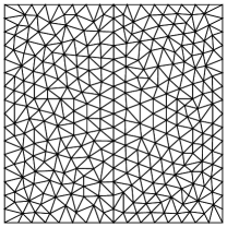
Figure 1: The triangulation of $\overline{\Omega}$ for $N=16$ used in Examples 1 and 2.

Example 1.

We consider the Oseen problem and the Navier–Stokes problem. Let $\Omega=(0,1)^{2}$, $T=1$. The functions $f$ and $u^{0}$ are defined so that the exact solution is

$$\begin{split}u_{1}(x,t)&=\phi(x_{1},x_{2},t),\\ u_{2}(x,t)&=-\phi(x_{2},x_{1},t),\\ p(x,t)&=C_{p}\sin(\pi(x_{1}+2x_{2})+1+t),\end{split}$$ (28)

where

$$\phi(a,b,t)=-\sin(\pi a)^{2}\sin(\pi b)\{\sin(\pi(a+t))+3\sin(\pi(a+2b+t))\}.$$

For the Oseen problem we set $w:=u$. We consider the four cases $\nu=10^{-2}$, $10^{-4}$, $C_{p}=1$, $10$.

For triangulations of domains FreeFem++ [18] is used. Let $N=16,23,32,45$ and $64$ be the division number of each side of $\overline{\Omega}$, and we set $h=1/N$. Figure 1 shows the triangulation of $\overline{\Omega}$ when $N=16$. The time increment $\Delta t$ is set to be $\Delta t=h^{2}$ so that we can observe the convergence behavior of order $h^{2}$. The purpose of the choice $\Delta t=O(h^{2})$ is to examine the theoretical convergence order, but it is not based on the stability condition. We set the stabilization parameter $\delta_{0}=10^{-1}$ for Schemes OsPstab and NSPstab.

The relative error $E_{X}$ is defined by

$$E_{X}(\phi)=\frac{\|\Pi_{h}^{(m)}\phi-\phi_{h}\|_{X}}{\|\Pi_{h}^{(m)}\phi\|_{X}},$$

for $\phi=u$ in $X=\ell^{\infty}(L^{2})$ and $\ell^{2}(H_{0}^{1})$ with $m=2$, and for $\phi=p$ in $X=\ell^{2}(L^{2})$ with $m=l$ when $\mathrm{P}_{2}/\mathrm{P}_{l}$-element is used. Here $\Pi_{h}^{(m)}$ is the Lagrange interpolation operator to the $\mathrm{P}_{m}$-finite element space. Table 1 shows the symbols used in graphs. Since every graph of the relative error $E_{X}$ versus $h$ is depicted in the logarithmic scale, the slope corresponds to the convergence order.

Table 1: Symbols used in Example 1.

$\phi$	$u$	$u$	$p$
$X$	$\ell^{\infty}(L^{2})$	$\ell^{2}(H^{1}_{0})$	$\ell^{2}(L^{2})$
TH	$\blacktriangle$	$\bullet$	$\blacksquare$
Pstab	$\vartriangle$	$\circ$	$\square$

Case (a)

Let $C_{p}=1$ in (28). We consider the Oseen problem and compare Schemes OsTH and OsPstab.

Figure 2: Case (a). Relative errors versus $h$ for $\nu=10^{-2}$ (left) and $\nu=10^{-4}$ (right).

Figure 2 shows the graphs of the errors $E_{\ell^{\infty}(L^{2})}(u)$ ($\blacktriangle$,$\vartriangle$), $E_{\ell^{2}(H^{1}_{0})}(u)$ ($\bullet$,$\circ$) and $E_{\ell^{2}(L^{2})}(p)$ ($\blacksquare$,$\square$) versus $h$. When $\nu=10^{-2}$, all convergence orders are almost two and there are no significant differences in both schemes.

When $\nu=10^{-4}$, the convergence orders of $E_{\ell^{\infty}(L^{2})}(u)$ ($\blacktriangle$,$\vartriangle$) are almost two in both schemes and there are no significant differences. The values of them are almost 1.5 times larger than those for $\nu=10^{-2}$. We also get results for $\nu=10^{-6}$, whose graph is omitted here, to observe that increases of the errors compared to $\nu=10^{-4}$ are less than two percent. The convergence order of $E_{\ell^{2}(H^{1}_{0})}(u)$ in Scheme OsTH ($\bullet$) is less than two, while the convergence order is almost two in OsPstab ($\circ$) and the value for $N=64$ is four times smaller than that in Scheme OsTH. In order to obtain the convergence order two in Scheme OsTH, finer meshes seem to be necessary. The convergence order of the error $E_{\ell^{2}(L^{2})}(p)$ ($\blacksquare$,$\square$) is almost two in both schemes and the values are almost same as those for $\nu=10^{-4}$. However, we do not have theoretical estimates for $p$ independent of the viscosity.

We observe that, although in Case (a) there are no significant differences between the both schemes in the errors $E_{\ell^{\infty}(L^{2})}(u)$ ($\blacktriangle$,$\vartriangle$), Scheme OsPstab shows higher accuracy for $\nu=10^{-4}$ in the errors $E_{\ell^{2}(H^{1}_{0})}(u)$ ($\circ$).

We consider the problem where the pressure value is larger.

Case (b)

Let $C_{p}=10$ in (28). We consider the Oseen problem and compare Schemes OsTH and OsPstab.

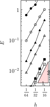
Figure 3: Case (b). Relative errors versus $h$ for $\nu=10^{-2}$ (left) and $\nu=10^{-4}$ (right).

Figure 3 shows the graphs of the errors. When $\nu=10^{-2}$, the values of $E_{\ell^{\infty}(L^{2})}(u)$ ($\blacktriangle$,$\vartriangle$) are almost same as Case (a). We observe differences in $E_{\ell^{2}(H^{1}_{0})}(u)$ in the two schemes. The values of errors in Scheme OsTH ($\bullet$) are about 1.5 times as large as those in Scheme OsPstab ($\circ$), and the values in the both schemes are about two to three times as large as in Case (a). The values of relative errors $E_{\ell^{2}(L^{2})}(p)$ ($\blacksquare$,$\square$) are, conversely, smaller than those in Case (a).

When $\nu=10^{-4}$, differences of the schemes appear more clearly in $E_{\ell^{\infty}(L^{2})}(u)$ and $E_{\ell^{2}(H^{1}_{0})}(u)$ than Case (a). The values of $E_{\ell^{\infty}(L^{2})}(u)$ in Scheme OsTH ($\blacktriangle$) are almost two to three times as large as those in Scheme OsPstab ($\vartriangle$). The values in Scheme OsPstab ($\vartriangle$) are almost 1.5 times larger than those for $\nu=10^{-2}$. We also get results for $\nu=10^{-6}$, whose graph is omitted here, to observe that increases of the errors compared to $\nu=10^{-4}$ are less than 15 percent. For $N=16$ and $23$ the values of $E_{\ell^{2}(H^{1}_{0})}(u)$ in Scheme OsTH ($\bullet$) are too large to be plotted in the graph, and for $N=32,45$ and $64$ the values are almost four to seven times as large as those in Scheme OsPstab ($\circ$). The values of relative errors $E_{\ell^{2}(L^{2})}(p)$ ($\blacksquare$,$\square$) are, conversely, smaller than those in Case (a).

We additionally consider the Navier–Stokes problems.

Case (c)

Let $C_{p}=1$ in (28). We consider the Navier–Stokes problem and compare Schemes NSTH and NSPstab.

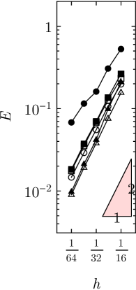
Figure 4: Case (c). Relative errors versus $h$ for $\nu=10^{-2}$ (left) and $\nu=10^{-4}$ (right).

Although in [33] numerical results of Scheme NSTH have already shown, we display them for the sake of completeness. Figure 4 shows the graphs of the errors. We observe the almost same behavior of the errors $E_{\ell^{\infty}(L^{2})}(u)$ ($\blacktriangle$,$\vartriangle$) and $E_{\ell^{2}(H^{1}_{0})}(u)$ ($\bullet$,$\circ$) as in Case (a) while the values of $E_{\ell^{2}(L^{2})}(p)$ ($\blacksquare$,$\square$) are almost 1.5 to 2 times as large as in Case (a).

Case (d)

Let $C_{p}=10$ in (28). We consider the Navier–Stokes problem and compare Schemes NSTH and NSPstab.

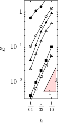
Figure 5: Case (d). Relative errors versus $h$ for $\nu=10^{-2}$ (left) and $\nu=10^{-4}$ (right).

Figure 5 shows the graphs of the errors. When $\nu=10^{-2}$, we observe the almost same behavior as in Case (b). When $\nu=10^{-4}$, the values of $E_{\ell^{\infty}(L^{2})}(u)$ ($\blacktriangle$,$\vartriangle$) and $E_{\ell^{2}(L^{2})}(p)$ ($\blacksquare$,$\square$) are almost two to four times as large as in Case (b), while the values of $E_{\ell^{2}(H^{1}_{0})}(u)$ ($\bullet$,$\circ$) are almost same as in Case (b).

Example 2.

In the Navier–Stokes problem we set

$$\Omega=(0,1)^{2},\quad T=40,\quad\nu=10^{-4},\quad f(x,t)=(0,10\sin(2\pi x_{2}))^{T},\quad u^{0}=0,$$

and compare Schemes NSTH and NSPstab.

We can easily check that the solution is $(u,p)(x,t)=(0,-\frac{5}{\pi}\cos(2\pi x_{2}))$. We use the mesh shown in Fig. 1 and take $\Delta t=0.01$. We set the stabilization parameter $\delta_{0}=10^{-3}$ for Scheme NSPstab.

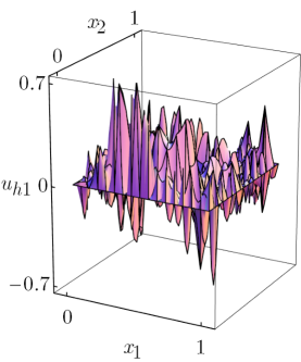
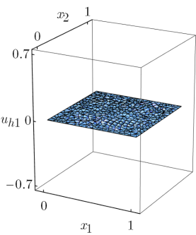
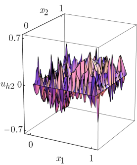
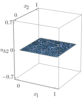
Figure 6: Example 2. Stereographs of $u_{h1}^{n}$ (top) and $u_{h2}^{n}$ (bottom) at $t^{n}=40$ by Scheme NSTH (left) and Scheme NSPstab (right).

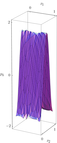
Figure 7: Example 2. Stereographs of $p_{h}^{n}$ at $t^{n}=40$ by Scheme NSTH (left) and Scheme NSPstab (right).

Figures 6 and 7 show the stereographs of the solutions $(u_{h}^{n},p_{h}^{n})$ at $t^{n}=40$ by the both schemes. In Scheme NSTH, oscillation is clearly observed for both components of the velocity and they are far from the constant zero, while in Scheme NSPstab the velocity is almost zero although small ruggedness is observed. For the pressure, difference between the two schemes is small compared to the velocity but the solution by Scheme NSPstab is better.

5 Concluding remarks

We constructed a pressure-stabilized Lagrange–Galerkin scheme for the Oseen problem with high-order elements, and showed an error estimate with the constant independent of the viscosity. The numerical examples showed the scheme has higher accuracy than the scheme with Taylor–Hood element especially for problems with small viscosity and large pressures. (i) Choice of the stabilization parameter in the pressure stabilization term, (ii) extension of the discussion to the Navier–Stokes problems, and (iii) numerical experiments of physically relevant problems will be future works.

Acknowledgements

The author would like to express his gratitude to Professor Emeritus Masahisa Tabata of Kyushu University for valuable discussions and encouragements. This work was supported by Japan Society for the Promotion of Science (JSPS) under Grant-in-Aid for JSPS Fellows, No. 26$\cdot$964, and under the Japanese-German Graduate Externship (Mathematical Fluid Dynamics), and by CREST, Japan Science and Technology Agency.

Appendix A Estimates for LG schemes

Lemma 5 is shown in [33, Lemma 5.7].

Lemma 5.

Let $w^{*}\in W^{1,\infty}(\Omega)^{d}$ and $X_{1}(w^{*})$ be the mapping defined in (4). Under the condition $\Delta t|w^{*}|_{1,\infty}\leq 1/4$, the estimate

$$\frac{1}{2}\leq\det\biggl{(}\frac{\partial X_{1}(w^{*})}{\partial x}\biggr{)}\leq\frac{3}{2}$$

holds, where $\det(\partial X_{1}(w^{*})/\partial x)$ is the Jacobian of $X_{1}(w^{*})$.

Lemma 6 is shown in [29, Lemma 1].

Lemma 6.

Let $w^{*}\in W^{1,\infty}_{0}(\Omega)^{d}$ and $X_{1}(w^{*})$ be the mapping defined in (4). Under the condition $\Delta t|w^{*}|_{1,\infty}\leq 1/4$, there exists a positive constant $c$ independent of $\Delta t$ such that for $v\in L^{2}(\Omega)^{d}$

$$\|v\circ X_{1}(w^{*})\|_{0}^{2}\leq(1+c|w^{*}|_{1,\infty}\Delta t)\|v\|_{0}^{2}.$$

We now show an estimate for $R_{1}^{n}$ in Lemma 7, or tools for estimating $R_{2}^{n}$ and $R_{3}^{n}$ in Lemmas 8 and 9, where $R_{i}^{n}$, $i=1,2,3$, are defined in (16). Although these estimates are frequently used in the analysis of the LG method, e.g. [25, 33], we show proofs of Lemmas 7 and 9 for completeness.

Lemma 7.

Suppose that $u\in Z^{2}$, $w\in C(W^{1,\infty}_{0})\cap H^{1}(L^{\infty})$ and $\Delta t|w|_{C(W^{1,\infty})}\leq 1/4$. Then

$$\|R_{1}^{n}\|_{0}\leq\sqrt{\Delta t}\left[\sqrt{\frac{2}{3}}(\|w^{n-1}\|_{0,\infty}^{2}+1)\|u\|_{Z^{2}(t^{n-1},t^{n})}+\left\|\frac{\partial w}{\partial t}\right\|_{L^{2}(t^{n-1},t^{n};L^{\infty})}\|\nabla u^{n}\|_{0}\right].$$

Proof.

We estimate $\|R_{1}^{n}\|_{0}$ by dividing

$$R_{1}^{n} =\left(\frac{\partial u^{n}}{\partial t}+(w^{n-1}\cdot\nabla)u^{n}-\frac{u^{n}-u^{n-1}\circ X_{1}(w^{n-1})}{\Delta t}\right)+\left((w^{n}\cdot\nabla)u^{n}-(w^{n-1}\cdot\nabla)u^{n}\right)$$

$$=:R_{11}^{n}+R_{12}^{n}.$$

For $R_{11}^{n}$, by setting

$$y(x,s):=x-sw^{n-1}(x)\Delta t,~{}t(s):=t^{n}-s\Delta t,$$

we use Taylor’s theorem to get

$$(u^{n-1}\circ X_{1}(w^{n-1}))(x)=u^{n}(x)-\Delta t\left(\frac{\partial u^{n}}{\partial t}+(w^{n-1}\cdot\nabla)u^{n}\right)(x)$$

$$\quad+\Delta t^{2}\int_{0}^{1}(1-s)\left(\frac{\partial}{\partial t}+w^{n-1}(x)\cdot\nabla\right)^{2}u(y(x,s),t(s))ds.$$

We then have

$$\|R_{11}^{n}\|_{0} \leq\Delta t\int_{0}^{1}(1-s)\left\|\left(\frac{\partial}{\partial t}+w^{n-1}(\cdot)\cdot\nabla\right)^{2}u(y(\cdot,s),t(s))\right\|_{0}ds$$

$$\leq\sqrt{2/3}\sqrt{\Delta t}(\|w^{n-1}\|_{0,\infty}^{2}+1)\|u\|_{Z^{2}(t^{n-1},t^{n})}.$$

where we have used the transformation of independent variables from $x$ to $y$ and $s$ to $t$, and the estimate $|\det(\partial x/\partial y)|\leq 2$ by virtue of Lemma 5. It is easy to show

$$\|R_{12}^{n}\|_{0}\leq\sqrt{\Delta t}\left\|\frac{\partial w}{\partial t}\right\|_{L^{2}(t^{n-1},t^{n};L^{\infty})}\|\nabla u^{n}\|_{0}.$$

Combining the two estimate, we have the conclusion. ∎

Lemma 8 is a direct consequence of [1, Lemma 4.5] and Lemma 5.

Lemma 8.

Let $1\leq q<\infty$, $1\leq p\leq\infty$, $1/p+1/p^{\prime}=1$ and $w_{i}\in W_{0}^{1,\infty}(\Omega)^{d}$, $i=1,2$. Under the condition $\Delta t|w_{i}|_{1,\infty}\leq 1/4$, it holds that, for $v\in W^{1,qp^{\prime}}(\Omega)^{d}$,

$$\|v\circ X_{1}(w_{1})-v\circ X_{1}(w_{2})\|_{0,q}\leq 2^{1/(qp^{\prime})}\Delta t\|w_{1}-w_{2}\|_{0,pq}\|\nabla v\|_{0,qp^{\prime}},$$

where $X_{1}(\cdot)$ is defined in (4).

Lemma 9.

Suppose that $v\in H^{1}(H^{1})$, $w^{*}\in W^{1,\infty}_{0}(\Omega)^{d}$, and $\Delta t|w^{*}|_{1,\infty}\leq 1/4$. Then

$$\left\|v^{n}-v^{n-1}\circ X_{1}(w^{*})\right\|_{0}\leq\sqrt{2\Delta t}\biggl{(}\left\|\frac{\partial v}{\partial t}\right\|_{L^{2}(t^{n-1},t^{n};L^{2})}+\|w^{*}\|_{0,\infty}\|\nabla v\|_{L^{2}(t^{n-1},t^{n};L^{2})}\biggr{)},$$

where $X_{1}(\cdot)$ is defined in (4).

Proof.

Similarly to the proof of Lemma 7 by defining

$$y(x,s):=x-sw^{*}(x)\Delta t,~{}t(s):=t^{n}-s\Delta t,$$

we have the estimate

$$\left\|v^{n}-v^{n-1}\circ X_{1}(w^{*})\right\|_{0}\leq\Delta t\int_{0}^{1}\left\|\left(\frac{\partial}{\partial t}+(w^{*}(\cdot)\cdot\nabla)\right)v(y(\cdot,s),t(s))\right\|_{0}ds.$$

The conclusion follows from the transformation of independent variables from $x$ to $y$ and $s$ to $t$, and the estimate $|\det(\partial x/\partial y)|\leq 2$ by virtue of Lemma 5. ∎

References

- [1] Y. Achdou and J.-L. Guermond. Convergence analysis of a finite element projection/Lagrange–Galerkin method for the incompressible Navier–Stokes equations. SIAM Journal on Numerical Analysis, 37(3):799–826, 2000.
- [2] R. Becker and M. Braack. A finite element pressure gradient stabilization for the Stokes equations based on local projections. Calcolo, 38(4):173–199, 2001.
- [3] M. Benzi, G.H. Golub, and J. Liesen. Numerical solution of saddle point problems. Acta Numerica, 14:1–137, 2005.
- [4] R. Bermejo and L. Saavedra. A second order in time local projection stabilized Lagrange–Galerkin method for Navier–Stokes equations at high Reynolds numbers. Computers and Mathematics with Applications, 72(4):820–845, 2016.
- [5] P.B. Bochev, C.R. Dohrmann, and M.D. Gunzburger. Stabilization of low-order mixed finite elements for the Stokes equations. SIAM Journal on Numerical Analysis, 44(1):82–101, 2006.
- [6] D. Boffi, F. Brezzi, and M. Fortin. Mixed Finite Element Methods and Applications. Springer, Berlin Heidelberg, 2013.
- [7] F. Brezzi and M. Fortin. A minimal stabilisation procedure for mixed finite element methods. Numerische Mathematik, 89(3):457–491, 2001.
- [8] F. Brezzi and J. Pitkäranta. On the stabilization of finite element approximations of the Stokes equations. In W. Hackbusch, editor, Efficient Solutions of Elliptic Systems, pages 11–19. Vieweg, 1984.
- [9] E. Burman. Pressure projection stabilizations for Galerkin approximations of Stokes’ and Darcy’s problem. Numerical Methods for Partial Differential Equations, 24(1):127–143, 2008.
- [10] E. Burman and M. A. Fernández. Galerkin finite element methods with symmetric pressure stabilization for the transient Stokes equations: Stability and convergence analysis. SIAM Journal on Numerical Analysis, 47(1):409–439, 2009.
- [11] P. G. Ciarlet. The Finite Element Method for Elliptic Problems, volume 40 of Classics in Applied Mathematics. SIAM, 2002.
- [12] Ph. Clément. Approximation by finite element functions using local regularization. RAIRO Analyse numérique, 9(2):77–84, 1975.
- [13] J. de Frutos, B. García-Archilla, V. John, and J. Novo. Grad-div stabilization for the evolutionary Oseen problem with inf-sup stable finite elements. Journal of Scientific Computing, 66(3):991–1024, 2016.
- [14] C. R. Dohrmann and P. B. Bochev. A stabilized finite element method for the Stokes problem based on polynomial pressure projections. International Journal for Numerical Methods in Fluids, 46(2):183–201, 2004.
- [15] J. Douglas, Jr. and Junping Wang. An absolutely stabilized finite element method for the Stokes problem. Mathematics of Computation, 52:495–508, 1989.
- [16] L.P. Franca and R. Stenberg. Error analysis of some Galerkin least squares methods for the elasticity equations. SIAM Journal on Numerical Analysis, 28(6):1680–1697, 1991.
- [17] R. Glowinski and P. Le Tallec. Augmented Lagrangian and Operator-Splitting Methods in Nonlinear Mechanics. SIAM, 1989.
- [18] F. Hecht. New development in FreeFem++. Journal of Numerical Mathematics, 20(3-4):251–265, 2012.
- [19] T. J. R. Hughes, L. P. Franca, and M. Balestra. A new finite element formulation for computational fluid dynamics: V. circumventing the Babuška–Brezzi condition: a stable Petrov–Galerkin formulation of the Stokes problem accommodating equal-order interpolations. Computer Methods in Applied Mechanics and Engineering, 59(1):85–99, 1986.
- [20] H. Jia, K. Li, and S. Liu. Characteristic stabilized finite element method for the transient Navier–Stokes equations. Computer Methods in Applied Mechanics and Engineering, 199(45–48):2996–3004, 2010.
- [21] V. John, A. Linke, C. Merdon, M. Neilan, and L.G. Rebholz. On the divergence constraint in mixed finite element methods for incompressible flows. SIAM Review, 59(3):492–544, 2017.
- [22] V. John and J. Novo. Analysis of the pressure stabilized Petrov–Galerkin method for the evolutionary Stokes equations avoiding time step restrictions. SIAM Journal on Numerical Analysis, 53(2):1005–1031, 2015.
- [23] H. Notsu. Numerical computations of cavity flow problems by a pressure stabilized characteristic-curve finite element scheme. Transactions of the Japan Society for Computational Engineering and Science, 2008. ONLINE ISSN: 1347-8826.
- [24] H. Notsu and M. Tabata. A combined finite element scheme with a pressure stabilization and a characteristic-curve method for the Navier-Stokes equations. Transactions of the Japan Society for Industrial and Applied Mathematics, 18(3):427–445, 2008. (In Japanese.).
- [25] H. Notsu and M. Tabata. Error estimates of a pressure-stabilized characteristics finite element scheme for the Oseen equations. Journal of Scientific Computing, 65(3):940–955, 2015.
- [26] H. Notsu and M. Tabata. Error estimates of a stabilized Lagrange–Galerkin scheme for the Navier–Stokes equations. ESAIM: Mathematical Modelling and Numerical Analysis, 50(2):361–380, 2016.
- [27] M.A. Olshanskii and A. Reusken. Grad-div stablilization for Stokes equations. Mathematics of Computation, 73:1699–1718, 2004.
- [28] O. Pironneau. On the transport-diffusion algorithm and its applications to the Navier-Stokes equations. Numerische Mathematik, 38(3):309–332, 1982.
- [29] H. Rui and M. Tabata. A second order characteristic finite element scheme for convection-diffusion problems. Numerische Mathematik, 92(1):161–177, 2002.
- [30] D. Silvester. Optimal low order finite element methods for incompressible flow. Computer Methods in Applied Mechanics and Engineering, 111(3–4):357–368, 1994.
- [31] E. Süli. Convergence and nonlinear stability of the Lagrange-Galerkin method for the Navier-Stokes equations. Numerische Mathematik, 53(4):459–483, 1988.
- [32] M. Tabata and S. Uchiumi. A genuinely stable Lagrange–Galerkin scheme for convection-diffusion problems. Japan Journal of Industrial and Applied Mathematics, 33(1):121–143, 2016.
- [33] M. Tabata and S. Uchiumi. An exactly computable Lagrange–Galerkin scheme for the Navier–Stokes equations and its error estimates. Mathematics of Computation, 87:39–67, 2018.
- [34] K. Tanaka, A. Suzuki, and M. Tabata. A characteristic finite element method using the exact integration. Annual Report of Research Institute for Information Technology of Kyushu University, 2:11–18, 2002. (In Japanese.).