A memory based random walk model to understand diffusion in crowded heterogeneous environment

Abstract

We study memory based random walk models to understand diffusive motion in crowded heterogeneous environment. The models considered are non-Markovian as the current move of the random walk models is determined by randomly selecting a move from history. At each step, particle can take right, left or stay moves which is correlated with the randomly selected past step. There is a perfect stay-stay correlation which ensures that the particle does not move if the randomly selected past step is a stay move. The probability of traversing the same direction as the chosen history or reversing it depends on the current time and the time or position of the history selected. The time or position dependent biasing in moves implicitly corresponds to the heterogeneity of the environment and dictates the long-time behavior of the dynamics that can be diffusive, sub or super diffusive. A combination of analytical solution and Monte Carlo simulation of different random walk models gives rich insight on the effects of correlations on the dynamics of a system in heterogeneous environment.

I INTRODUCTION

Diffusion has always been a subject of interest due to its wide applicability in physics, chemistry and biology Frey and Kroy (2005); Hasnain, Jacobson, and Bandyopadhyay (2014); George and Thomas (2001); Kastantin, Walder, and Schwartz (2012); Plastino et al. (2004). The diffusion of molecules can be under the influence of concentration gradient or because of thermal motion of the molecules. The diffusive motion of particles can be categorized as normal or anomalous depending on the variation of mean square displacement (MSD) with time (t). The diffusion is said to be normal when MSD varies linearly with time i.e. $MSD\propto t$. However, when the MSD varies with t as $MSD\propto t^{\alpha}$($\alpha$ is called the diffusion exponent) and $\alpha\neq 1$, diffusion is said to be anomalous. When $0<\alpha<1$, the diffusion is said to be subdiffusive and it is superdiffusive when $\alpha>1$. The subdiffusive dynamics can be due to crowding in a concentrated system which can make the system heterogeneous and disordered Ghosh et al. (2016). The crowded environment obstructs the diffusing particle and generally gives rise to subdiffusion Vercammen, Maertens, and Engelborghs (2007); Pan et al. (2009); Szymanski and Weiss (2009); Ernst et al. (2012); Jeon et al. (2013); Grebenkov et al. (2013); Grebenkov and Vahabi (2014); Ernst, Köhler, and Weiss (2014); Lee et al. (2014); Shin, Cherstvy, and Metzler (2015). Biological systems are good examples of crowded and heterogeneous environments and have been extensively studied Höfling and Franosch (2013); Jeon et al. (2011); Seisenberger et al. (2001); Skaug, Faller, and Longo (2011); Weigel et al. (2011); Sahl et al. (2010); Hasnain et al. (2014); McGuffee and Elcock (2010); Nicolau, Hancock, and Burrage (2007); Janmey et al. (1986); Xie et al. (2008); Hammar et al. (2012). Experimental studies confirmed the presence of subdiffusion while studying the motion of macromolecules inside different biological cells Golding and Cox (2006); Weiss et al. (2004); Banks and Fradin (2005); Kues, Peters, and Kubitscheck (2001); Brown et al. (1999); Wachsmuth, Waldeck, and Langowski (2000). However, the observed subdiffusion can be a transient one, meaning that the subdiffusion $\alpha<1$ becomes normal $\alpha=1$ at long time, or a persistent one, where $\alpha$ always remains less than one.
Experimental signatures of both transient and persistent subdiffusion have been observed. For instance, in the experimental study by Golding and Cox Golding and Cox (2006), the motion of fluorescently labeled mRNA molecule has been tracked inside a live E. coli cell and is found to be persistently subdiffusive with MSD varying as $MSD\propto t^{0.70}$ . The studies mentioned in references Skaug, Faller, and Longo (2011); Golding and Cox (2006); Banks and Fradin (2005); Brown et al. (1999); Wachsmuth, Waldeck, and Langowski (2000) confirm the presence of persistent subdiffusion with constant diffusion exponent over all time scales. Transient subdiffusion has been observed by Javanainen et al. Javanainen et al. (2013) in the study of lateral diffusion of proteins in a crowded lipid membrane. Similar results have also been found in references Berezhkovskii, Dagdug, and Bezrukov (2014a, b) and Hasnain et al. (2014). In a recent work Jeon et al. (2016), extensive molecular dynamics simulations have been performed to determine the effect of protein crowding on membrane dynamics. The simulation study of lipids in the presence of protein or cholesterol as crowding particles shows persistent anomalous subdiffusion dynamics for both lipids and membrane-embedded proteins, which is governed by a non-Gaussian distribution Metzler, Jeon, and Cherstvy (2016).
Theoretical models like Fractional Brownian motion Mandelbrot and Van Ness (1968), Continuous time random walk, Metzler and Klafter (2000) and Obstructed diffusion Havlin and Ben-Avraham (1987) have been utilized by previous studies to understand subdiffusion in crowded environment. Mandelbrot and Van Ness Mandelbrot and Van Ness (1968) showed that when the direction of motion of a particle is determined from the history in a power law fashion, which can be either correlated or anti-correlated, diffusion is found to be anomalous and is termed as Fractional Brownian Motion. The origin of anomaly in this case is long-range temporal rather than spatial correlation. Power laws occur frequently in the diffusion in heterogeneous environments with multi-scale features but differing in their origin Fish (2010); Coppens and Dammers (2006). Previously Hasnain et al. Hasnain et al. (2014) found transient subdiffusion for protein diffusion in a cytoplasm. The random walk model described in reference Hasnain and Bandyopadhyay (2015) is appropriate for transient sub-diffusion in crowded environment but not for describing persistent sub-diffusion.
In the current work, we study microscopic random walk models to describe persistent subdiffusion in heterogeneous environment. The main motivation behind our study is to incorporate effects of dynamic heterogeneity to the existing model by introducing dynamic correlations between the current step and the history. Our starting point is the model developed by Kumar et al. Kumar, Harbola, and Lindenberg (2010)(henceforth this model will be referred as Kumar’s model). In that model, the authors developed a memory based random walk model in which the current step depends on the randomly selected past step. At each step, the particle can take one of the three steps; left, right and stay (i.e. does not move). In the model, the stay moves are perfectly correlated which implies that if the past step selected is a stay move, then the particle will stay at its position with probability one. However, if the past step selected is right (left), the particle has the probability to take right (left) move with probability ‘p’ or chooses to reverse its direction with probability ‘q’. It can also stay at its position with probability ‘r’. The parameters ‘p’ and ‘q’ are taken as constants and are independent of the current step and the past step selected. The model can describe all types of diffusion, namely superdiffusion, normal and subdiffusion. In a similar work by Harbola et al. Harbola, Kumar, and Lindenberg (2014), the authors proposed a minimal- option model for the walker. A walker can take either forward or stay move with perfect correlation in the stay moves. The model also shows all types of diffusion such as subdiffusive, superdiffusive and normal. However, the random walk models discussed above Kumar, Harbola, and Lindenberg (2010); Harbola, Kumar, and Lindenberg (2014) do not account for the heterogeneity of the environment and its effect on the dynamics of particle. In the present work, we show that the heterogeneity of the environment can give rise to qualitative changes in dynamics which has not been discussed in previous literature.
In the current work, we have implicitly included the effects of heterogeneity of the system and crowding on the dynamics of diffusing particle both in an average manner and as local crowding. First, the average crowding in the environment has been included by allowing the particle to stay at the current position with probability (r) which is the probability of the occupancy of the neighboring lattice sites. Secondly, the probabilities (p and q) to choose the direction of the next step are considered as functions of the current and the past times and positions (i.e. there are two different models for temporal and spatial dependence). This tries to take care of local (dynamic) crowding since the presence of local heterogeneity in the system may lead to spatial and temporal correlation between the past and present moves. The randomly chosen steps from immediate past are sometimes followed with lower probability than those chosen from the distant past and vice versa. The current model differs from Kumar’s model in the sense that, in the present model, the environment heterogeneity dynamically influences the efficiency with which the particle follows a past step. As we discuss below, this heterogeneity effect leads to qualitative changes in the dynamics predicted by the Kumar’s model.
One of the models proposed here give all three types of diffusion but the other two models give only subdiffusion. Hence, the dynamical behaviors depend on the type of correlation induced by heterogeneity. The paper is organized in the following manner. Methodology section describes Kumar’s model and our extension of it. In the method section, we have also given analytical formulation and Monte Carlo simulation schemes performed. Result section gives the features of the models using MSD, diffusion exponent ( $\alpha$) and probability distribution function (PDF). A summary of the three models and their connection to the heterogeneity of the environment has also been discussed. The paper ends with a conclusion and possible future work.

II METHODOLOGY

Several random walk models have been proposed to understand the mechanism of subdiffusion in crowded environment Metzler and Klafter (2000); Bouchaud and Georges (1990); Ben-Avraham and Havlin (2000); Metzler et al. (2014); Meroz and Sokolov (2015); Saxton (1997); Vilaseca et al. (2011); Isvoran et al. (2008). A simple random walk consists of a series of right and left moves along a one-dimensional lattice Chandrasekhar (1943) with equal probability which is independent of the previous steps taken. This type of motion with independent steps gives rise to normal diffusion at long times where MSD varies linearly with time. However, when the walk is biased in a direction, leading to drift in that direction, it is said to be a biased random walk Berg (1993). If the steps are correlated it is called a correlated random walk Montroll and Weiss (1965); Konno (2009) which may give rise to anomalous diffusion, i.e., subdiffusion and superdiffusion. Several theoretical and computational models have been developed in the past which can produce transient subdiffusion Hasnain et al. (2014); Berezhkovskii, Dagdug, and Bezrukov (2014a, b); Ando and Skolnick (2010); Ridgway et al. (2008) . However, only few microscopic models are known Kumar, Harbola, and Lindenberg (2010); Harbola, Kumar, and Lindenberg (2014) to explain normal diffusion, persistent subdiffusion and superdiffusion within the same scheme.

II.1 Kumar’s Model

This model consists of a random walker moving on a one-dimensional infinite lattice where the lattice points are unit distance apart. The starting step ($\sigma_{1}$) is selected in the right or left direction with probability s or (1-s), respectively where $s>0$ . The subsequent steps can be right, left or stay which is decided as the following. At each step, a past step is selected uniformly from the history which decides the current move of the particle. If the past step selected is a stay move, then the particle remains at the present position with probability 1. However, if the past step selected is right or left, then the particle has the tendency to move in the same or reverse direction with probability p and q, respectively. It can also stay in the same point with probability r. In this model p is said to be the probability of going in the same direction and q is the probability of reversing the direction and these values are taken as constants, independent of the current and past steps. At each step, the sum of p, q and r should be equal to 1. The model gives subdiffusion, superdiffusion and normal diffusion depending on the asymmetry parameter $\gamma$ where $\gamma=p-q$ . The position $x_{n+1}$ of the particle at step n+1 is given as ( $x_{n}$ is the position after step n)

$$x_{n+1}=x_{n}+\sigma_{n+1}$$ (1)

where $\sigma_{n+1}=\pm 1,0$ is the current move at ${n+1}^{th}$ step which is decided from a randomly selected past step from the history $\left\{\sigma_{1},\sigma_{2},\sigma_{3},....,\sigma_{n}\right\}$ with uniform probability 1/n. For the first step, $\sigma_{1}=\pm 1$
If $\sigma_{k}$ is the randomly selected past step, then
$\sigma_{n+1}=\sigma_{k}$ with probability p
$\sigma_{n+1}=-\sigma_{k}$ with probability q
$\sigma_{n+1}=0$ with probability r
It is crucial to have perfect correlation between the stay moves, otherwise only normal and transient subdiffusive or superdiffusive dynamics is predicted by this model Harbola, Kumar, and Lindenberg (2014).
The random walk with the given probabilities can be described as the following. For the first step at time t=1, the probability that $\sigma_{1}=\sigma$ is given by

$$P[\sigma_{1}=\sigma]=\frac{1}{2}[1+(2s-1)\sigma]\,,\mbox{where}\,\sigma=\pm 1$$ (2)

For time t+1 ($t\geq 1$), the conditional probability to make a move $\sigma(=1,-1,0)$ is given as

$$P[\sigma_{t+1}=\sigma|{\sigma_{t}}]=1-\sigma^{2}+\frac{1}{2t}\sum_{k=1}^{t}\sigma_{k}^{2}(3\sigma^{2}-2)(1-r)+\sigma\sigma_{k}\gamma$$ (3)

Here $\gamma=p-q$ . Using Eq. 3, the first two moments of the displacement after time t can be obtained as shown in previous works Kumar, Harbola, and Lindenberg (2010); Harbola, Kumar, and Lindenberg (2014).

II.2 Extension of Kumar’s model to incorporate environmental heterogeneity

In the current work, we are proposing a model to understand anomalous diffusion in complex heterogeneous environment. In our model, we associate the stay probability (r) to the occupancy of the lattice sites i.e. the fractional volume occupancy of a crowded system. This implicitly includes the effect of crowding in an average manner. In Kumar’s model p and q are constants which do not describe the heterogeneity of the environment of the diffusing particle. To account for the heterogeneity of the environment, we consider p and q as functions of current time t, and the history selected. Note that the time t is analogous to the step number. The time dependence of p and q accounts for the local heterogeneity of the system. We have kept r fixed for a particular study so only one independent parameter p (or q) is required to specify the model. For the current study we have taken three different cases for the selection of probability p which are given below

II.2.1 Model 1:

$$p(t,k)={(\frac{t-k}{t})}^{\beta}(1-r)\,\mbox{,where}\,\beta>0$$ (4)

where $t$ is the current time, $k$ is the time of randomly selected past step, r is the stay probability and $\beta$ is a parameter determining the heterogeneity of the environment. From the above expression, it can be said that $p(t,k)$ will have higher value when the selected step k is far from the present time compared to the case where k is close to the present time. The parameter $\beta$ determines how efficiently particle follows the past i.e. in this case the far history is followed with more probability than the close one.

II.2.2 Model 2:

$$p(t,k)={\exp{(-(t-k)^{2})}}(1-r)$$ (5)

This represents a Gaussian time-correlation between present and past selected moves. From the above expression, it can be said that $p(t,k)$ with a randomly selected step closer to the present time has higher value than the other case.

II.2.3 Model 3:

$$p(t,k)=(1+(t-k)^{2})^{-\epsilon}(1-r)$$ (6)

where $\epsilon$ is a parameter having value greater than zero. This model also shows that $p(t,k)$ will have larger value for randomly selected step close to the current state.
For the above three models, $p(t,k)$ is a function of time only and hence we call it as temporal dependence henceforth. However, we shall also analyze the cases when probabilities of taking moves are functions of positions at times t and k . We shall call this as spatial dependence. For brevity, henceforth we shall write $p(t)$ (or $p(x)$, when it is a function of position) as p only.
Let $p(t,k)[q(k,t)]$ be the probability to follow [reverse] a randomly chosen $k^{th}$ step at time $t$, if $\sigma_{k}=\pm 1$. Then the conditional probability, $P[\sigma_{t+1}=+1|\{\sigma_{t}\}]$, to have step $\sigma_{t+1}=+1$ for a given history $\{\sigma_{t}\}$ can be written as,

$$P[\sigma_{t+1}=+1|\{\sigma_{t}\}]=\frac{1}{t}\sum_{k=1}^{t}\left[\delta_{\sigma_{k},+1}p(t+1,k)+\delta_{\sigma_{k},-1}q(t+1,k)\right]$$ (7)

where $\delta_{\sigma_{k},\pm 1}$ is the kronecker delta function between $\sigma_{k}$ and $\pm 1$. Since $\sigma_{k}=\pm 1$ or $0$, we can re-express the above equation in terms of $\sigma_{k}$ as,

$$P[\sigma_{t+1}=+1|\{\sigma_{t}\}]=\frac{1}{2t}\sum_{k=1}^{t}\sigma_{k}\left[(1+\sigma_{k})p(t+1,k)-\sigma_{k}(1-\sigma_{k})q(t+1,k)\right]$$ (8)

This can be rearranged to

$$P[\sigma_{t+1}=+1|\{\sigma_{t}\}]=\frac{1}{2t}\sum_{k=1}^{t}\left(\frac{}{}\sigma_{k}^{2}[p(t+1,k)+q(t+1,k)]+\sigma_{k}[p(t+1,k)-q(t+1,k)]\frac{}{}\right)$$ (9)

Similarly, for $P[\sigma_{t+1}=-1|\{\sigma_{t}\}]$, we obtain,

$$P[\sigma_{t+1}=-1|\{\sigma_{t}\}]=\frac{1}{2t}\sum_{k=1}^{t}\left(\frac{}{}\sigma_{k}^{2}[p(t+1,k)+q(t+1,k)]-\sigma_{k}[p(t+1,k)-q(t+1,k)]\frac{}{}\right)$$ (10)

Since $P[\sigma_{t+1}=0|\{\sigma_{t}\}]=1-P[\sigma_{t+1}=+1|\{\sigma_{t}\}]-P[\sigma_{t+1}=-1|\{\sigma_{t}\}]$, one obtains,

$$P[\sigma_{t+1}=0|\{\sigma_{t}\}]=1-\frac{1-r}{t}\sum_{k=1}^{t}\sigma_{k}^{2}.$$ (11)

We can combine Eqs. (9)-(11) in to a single equation as,

$$P[\sigma_{t+1}=\sigma|\{\sigma_{t}\}]=1-\sigma^{2}+\frac{1-r}{2t}\sum_{k=1}^{t}\left[\frac{}{}(3\sigma^{2}-2)\sigma_{k}^{2}+\frac{\sigma\sigma_{k}}{1-r}(2p(t+1,k)-1+r)\frac{}{}\right]$$ (12)

where $\sigma=0,\pm 1$. Several things can be derived starting from Eq. (12). Let $p_{\pm}(t)$ be the probability of the $t^{th}$ step to be $\pm 1$, and similarly $p_{0}(t)$ for the $t^{th}$ step to be zero. These probabilities are then obtained by averaging Eq. (12) over all histories. For example,

$$p_{\pm 1}(t+1)=\frac{1-r}{2t}\sum_{k=1}^{t}\left[\frac{}{}\langle\sigma_{k}^{2}\rangle+\frac{\sigma\langle\sigma_{k}\rangle}{1-r}(2p(t+1,k)-1+r)\frac{}{}\right]$$ (13)

Note that averages, $\langle\sigma_{k}\rangle$ and $\langle\sigma_{k}^{2}\rangle$ can be expressed in terms of $p_{\pm}(k)$ as $\langle\sigma_{k}\rangle=p_{+}(k)-p_{-}(k)$ and $\langle\sigma_{k}^{2}\rangle=p_{+}(k)+p_{-}(k)$. Using this in Eq. (13) and the fact that $p_{0}(t)=1-p_{+}(t)-p_{-}(t)$, we obtain a recursive relation for $p_{0}(t)$,

$$p_{0}(t)=\frac{r}{t-1}+\frac{t-r-1}{t-1}p_{0}(t-1).$$ (14)

It can be solved to obtain,

$$p_{0}(t)=1-\frac{\Gamma(t-r)}{\Gamma(t)\Gamma(1-r)}$$ (15)

where $\Gamma$ refers to the gamma function and $t>1$. This immediately gives,

$$p_{+}(t)+p_{-}(t)=\frac{\Gamma(t-r)}{\Gamma(t)\Gamma(1-r)}$$ (16)

when $t>1$. We next start from Eq. (13) to calculate $\Delta p(t)=p_{+}(t)-p_{-}(t)$. We get,

$$\Delta p(t+1)=\frac{1}{t}\left[2p(t+1,t)+r+t-2\right]\Delta p(t)+\frac{2}{t}\sum_{k=1}^{t-1}\Delta p(k)[p(t+1,k)-p(t,k)].$$ (17)

Since $\Delta p(1)=2s-1$, from Eq. (17), all $\Delta p(k)$ are proportional to $2s-1$. Thus for $s=1/2$, $\Delta p(k)=0~{}\forall k>0$. Thus for $s=1/2$,

$$p_{+}(t)=p_{-}(t)=\frac{\Gamma(t-r)}{2\Gamma(t)\Gamma(1-r)}.$$ (18)

Indeed this immediately leads to

$$\langle\sigma_{k}\rangle = 0$$ (19)

$$\langle\sigma_{k}^{2}\rangle = \frac{\Gamma(k-r)}{\Gamma(k)\Gamma(1-r)}$$ (20)

and therefore $\langle x_{t}\rangle=0$ $\forall$ t. Because of the complexity of the expressions, it has not been possible to derive the expression for the second moment of displacement. The second moment of displacement has been calculated numerically using Monte Carlo simulation scheme.

II.3 Monte Carlo Simulations

Because of the complexity of the models in the current work, we have used Monte Carlo (MC) simulations to the dynamic behavior for different models as given in Eq. 4-6. For each model, corresponding to each walk length, we have run 9 million MC simulations. The MSD and diffusion exponent ($\alpha$) have been calculated for each model. From each case, our focus is on understanding the diffusive behavior at different values of volume occupancy (given by r) and the environmental heterogeneity (given by the time or spatial dependence of p and q). For comparison, we have run MC simulations for Kumar’s model with the appropriate parameters. For $p-q<0$, Kumar’s model Kumar, Harbola, and Lindenberg (2010) always gives rise to subdiffusion with $\alpha=1-r$. For comparison, we took p=0.2 and q=0.6 and the stay probability, r=0.2 for Kumar’s model to compare the models developed in our work (where stay probability r is taken as 0.2). Our models’ p and q are determined from Eqs. 4-6 corresponding to model 1, 2 and 3 respectively.
In the next section, we discuss simulation results for each model and make comparison with Kumar’s model wherever possible.

III RESULTS

III.1 Model 1

For model 1, we have calculated the second moment of displacement for different values of stay probability ‘r’ and heterogeneity parameter ‘$\beta$’. Figure 1 shows mean square displacement (MSD) plotted againt N for stay probability r=0.2, 0.4 and heterogeneity parameter $\beta=1.0.,2.0$. Figure shows decrease in the value of MSD with increase in heterogeneity parameter and stay probability. With increase in the value of $\beta$, the probability of reversing the history increases with leads to the decrease in the value of MSD.

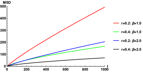
Figure 1: Figure shows MSD, obtained from model 1, plotted against time (t) at stay probability (r=0.2, 0.4) and heterogeneity parameter ($\beta=1.0,2.0$).

In Fig. 2, we show the diffusion exponent ($\alpha$) plotted against time (t) for r=0.2, 0.4 and $\beta=0.1,0.9$. We observe that, initially, the diffusion exponent decreases with increase in t (except for the blue curve, which increases at short time), until it converges to some constant value. For r=0.2, superdiffusive motion (with $\alpha=1.38$) is observed at $\beta=0.1$ and is subdiffusive (with $\alpha=0.88$) at $\beta=0.9$. Similar qualitative behavior is observed for r=0.4, that is superdiffusive (with $\alpha=1.08$) at $\beta=0.1$ and is subdiffusive (with $\alpha=0.74$) at $\beta=0.9$.
For a given value of r the dynamics changes significantly with change in value of $\beta$ . The change in $\beta$ , implicitly representing the heterogeneity of the environment, is leading to qualitative changes in dynamics. Figure 2 also shows comparison of the current model with Kumar’s model for two values of stay probability. From Kumar’s model, for r=0.2, persistent subdiffusion is observed with exponent $\alpha=1-r=0.8$ when $p-q<0$. From the current model, at r=0.2 we get superdiffusion, normal (not shown in the figure) or subdiffusion with exponent depending on value of $\beta$ which incorporates effect of environment. Similarly, for r=0.4, we see a qualitative effect of heterogeneity which changes the long-time dynamics from superdiffusion, at $\beta=0.1$, to subdiffusion, at $\beta=0.9$, and differentiates the dynamics from Kumar’s model Kumar, Harbola, and Lindenberg (2010).

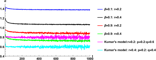
Figure 2: Figure shows diffusion exponent ($\alpha$), for model 1, plotted against time (t) for different values of stay probability (r) and heterogeneity parameter ($\beta$).

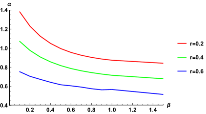
Figure 3: Figure shows variation of diffusion exponent ($\alpha$) for model 1 plotted against heterogeneity parameter ($\beta$) for different values of stay probability (r).

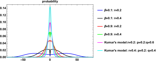
Figure 4: Figure shows probability distribution function for walk of length t=100 steps at different values of stay probability (r) and heterogeneity parameter ($\beta$) obtained under model 1.

In Fig. 3, we show simulation results for diffusion exponent ($\alpha$) plotted against $\beta$ for different values of r. The exponent $\alpha$ decreases with increase in $\beta$ . For small values of $\beta$ , $\alpha$ decreases sharply and then gradually settles to a constant value. For r=0.2 and r=0.4, we see qualitative change in the dynamics with increase in the value of beta. For smaller values of $\beta$ motion is superdiffusive and it goes to subdiffusive as $\beta$ value increases. For any given value of volume occupancy (r), increase in the parameter $\beta$ leads to a decrease in ‘p’ and consequently increase in the value of ‘q’. The increase in the value of ‘q’ allows the particle to reverse its direction more for any chosen history, which can shift the qualitative behavior of diffusion from superdiffusive to subdiffusive as shown in figure 3. However, for large volume occupancy r=0.6, we observe subdiffusive motion for all values of $\beta$. We next look at the heterogeneity effects on the full probability distribution of position of the walker. In Fig. 4, we show PDF for different values of stay probability (r) and heterogeneity parameter ($\beta$) for walks of length up to 100 steps obtained from MC simulations. The distribution is symmetric around the origin with two peaks on each side of the origin. The symmetry is due to the choice $s=1/2$ which implies that the probabiility of the first step is taken as $1/2$ in both right and left direction. With the increase in the stay probability r, the distribution becomes more and more peaked around the origin with two peaks getting closer to each other, and the dip at the origin becomes deeper. An increase in $\beta$ also makes the distribution more confined around the origin. This is understandable as diffusion becomes slower ($\alpha$ decreases) with increase in r and $\beta$. To understand the dip at x=0 we consider the extreme case when $\beta=0$ which gives $p(t)=(1-r)$ i.e. $q(t)=0.0$ (see Eq 4). This makes the particle to move in the direction of the first step which is always away from the origin ($\sigma_{1}=\pm 1$), giving zero probability for particle to be at x=0. With increase in the value of $\beta$, the probability of reversing direction increases in time which increases the probability at position x=0 but is always less than its neighboring positions which are more probable. The figure also shows PDF obtained from Kumar’s model at r=0.2 and 0.4 at p=0.2. From the figure, we see that for a given value of ‘r’, the distributions obtained from Kumar’s model are more peaked than the one obtained from our model at different values of parameter $\beta$. The difference in PDF is due to the change in the value of ‘p’ due to the heterogeneity parameter in our model, unlike Kumar’s model which has a constant value of ‘p’.

III.2 Model 2

The MC simulations have been performed using Eq.5 as the probability of following a randomly selected past step. The probability of following or reversing the selected history depends on the current time (t) and the history selected ( k ). Figure 5 shows diffusion exponent ($\alpha$) , obtained from MC simulations, plotted against time (t) at r=0.2 and r=0.4 . From the figure, we see that the diffusion exponent ($\alpha$) in each cases converges to 1-r with increase in time ‘t’. The dynamics for this model is similar to Kumar’s model with $p-q<0.5$ and $r<1-2(p-q)$ where the motion is subdiffusive with exponent $\alpha=1-r$. With increase in time, the difference $t-k$ increases, which causes decrease in value of ‘p’. The value of ‘p’ at somes point becomes negligible in comparison to q (=1-p-r) which corresponds to subdiffusive ($\propto t^{(1-r)}$) kind of dynamics mentioned in reference Kumar, Harbola, and Lindenberg (2010).

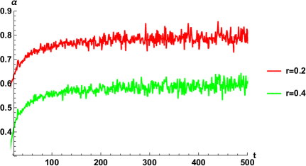
Figure 5: Figure shows variation of diffusion exponent ($\alpha$) for model 2 plotted against time (t) for different values of stay probability (r).

Using MC simulations, we also study the case when the probability of following a selected history, p, is a function of the current position and the position at the randomly selected history. The walk with space dependent probability, p(x), is termed here as spatially correlated walk. The spatial correlation was not considered for model 1 because the function p(x) is not defined if the particle is at x=0 at any time. For spatially correlated walk, the probability of following the selected past step is defined as

$$p=\exp(-(x(t-1)-x(k))^{2})(1-r)$$ (21)

where $x(t)$ is the position at time t. Note that with this form, p becomes more fluctuating quantity than its temporal counterpart.

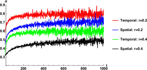
Figure 6: Figure shows variation of diffusion exponent ($\alpha$) for spatial and temporal correlated walks under model 2 plotted against time (t) for different values of stay probability (r).

Figure 6 shows time dependence of the diffusion exponent for the spatially and the temporally correlated dynamics at r=0.2 and r=0.4. For both spatial and temporal correlations, the increase in volume occupancy ‘r’ gives rise to more subdiffusive behavior with smaller value of diffusion exponent $\alpha$ as shown in the figure. For spatial dependence, diffusion exponent is found to be lower than temporal dependence. At any time, t, x(t)-x(k) is less than or equal to t-k which makes the probability ‘p’ for spatially correlated walk to be larger than temporally correlated one, $p(x(t))>p(t)$, the effect of which is observed in simulations. For temporal correlated walk, diffusion exponent $\alpha$ converges to $1-r$ at long time unlike the spatial correlated walk which converges to lower value. The exponent in case of spatial correlated walk is not just dependent on r but also the values of p and q. Figure 7 compares probability distribution function for the spatially and the temporally correlated walks. For points farther from the origin, probability for spatial dependent walk is more than that of temporal dependent walk. Since $p(x(t))>p(t)$, this may account for the higher probability for points far from the origin. On the other hand, probability conservation requires that the points close to the origin have comparatively less probability, as seen in the figure. The probability of finding the walker at any position x(t) at time t depends both on number of paths leading to that position and the probability of each path. For position x=0, the number of paths are always larger than its neighboring position but the sum of probabilities of paths is less than those of the neighboring positions, which leads to a dip at x=0. Figure also shows PDF obtained from Kumar’s model at r=0.2 and r=.4 and p=0.2. For temporal correlated walk (in each case r=0.2 and r=0.4), the PDF is closer to the one obtained from Kumar’s model but have higher peak at the mean position and less displacement around the mean position. The difference in the distribution is due to the difference in ‘p’ values in the current model and in Kumar’s model. In the current model, unlike Kumar’s model ‘p’ changes at each step and is a function of current step and the history selected which in general decreases with time leading to more direction reversal and more confined motion around the mean position.

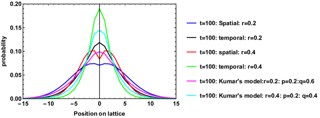
Figure 7: Figure shows probability distribution function for walk of length t=100 steps for model 2 using spatial and temporal correlations at stay probability r=0.2 and r=0.4

III.3 Model 3

The MC simulations have been performed using p given in Eq. 6, where $\epsilon$ is a parameter that determines change in the value of p with time. MSD and $\alpha$ are calculated from the simulation. Figure 8 shows changes in $\alpha$ against time t as obtained from MC simulations at $\epsilon=1$ and $\epsilon=2$. For a fixed value of r, dynamics changes significantly with $\epsilon$. However, this change is significant only over the transient dynamics. The diffusion exponent ($\alpha$) approaches the value 1-r asymptotically for the given values of $\epsilon$ , as shown in figure. For small values of $\epsilon$ , it takes longer time to reach the constant $\alpha$ value. For all values of $\epsilon$ considered, model 3, similar to model 2, gives only subdiffusion with exponent, $\alpha=1-r$. This is due to the decrease in the value of ‘p’ with increase in time and hence results in increase in the value of ‘q’. The subdiffuive dynamics with exponent exponent $1-r$ is in accordance with the Kumar’s model when $p-q<0.5$.
We next consider spatial correlation for model 3. The corresponding probability p for spatial correlated walk is given as

$$p=(1+(x(t-1)-x(k))^{2})^{(-\epsilon)}(1-r)$$ (22)

Using Eq. 22 for the biasing probability ‘$p$’ we performed MC simulations to calculate MSD and diffusion exponent ($\alpha$ ) for walks of lengths up to 1000 steps.
Figure 9 shows comparison of $\alpha$ values for spatial and temporal correlations at $\epsilon=1/6,r=0.2$. For temporal correlated walk, the diffusion exponent ($\alpha$) first decreases and then increases till it attains diffusion exponent $\sim 0.7$ within the given time interval of time(however at long time as mentioned it goes to 1-r). However, for spatial correlated walk, diffusion exponent decrease monotonically till it reaches a constant value $\sim 0.5$ . The exponent value in case of spatially correlated walk is found to be lower than the temporal correlated walk. However, for spatial correlated walk the value of p is larger than the temporally correlated walk. For spatial correlation, it is expected that the change in value of p is slower in case of temporally correlated walk which is due the fact that number of distinct positions covered (from time $1$ to $t-1$) is always less than the number of time steps covered (history positions are very few in comparison to time of history which is from $1$ to $t-1$). The slow rate of decrease of p is also responsible for slow rate of increase of MSD with time. The slow rate of change of MSD suggests higher subdiffusive behavior in spatial correlated walk in comparison to temporal correlated walk. Figure 9 also shows comparison of diffusion exponent ($\alpha$) from the given model and Kumar’s model at stay probability of 0.2. From the figure, it can be seen for same value of $\epsilon$ spatial correlation gives lower value of $\alpha$ in comparison to temporal correlation and Kumar’s model at stay probability of 0.2.

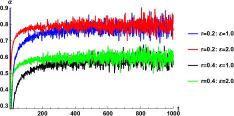
Figure 8: Figure shows variation of diffusion exponent ($\alpha$) for model 3 plotted against time (t) for stay probability r=0.2 and r=0.4 with heterogeneity parameter $\epsilon=1.0$ and $\epsilon=2.0$.

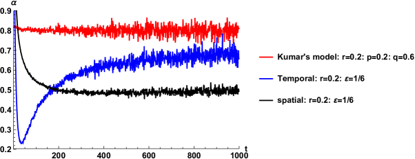
Figure 9: Figure shows variation of diffusion exponent ($\alpha$) for model 3 plotted against time (t) at $\epsilon=1/6$ for both spatial and temporal correlated walk at stay probability r=0.2.

Summary of the models

The models discussed in this work for the probability of following the past step hold importance in the dynamics of a particle. The model 1 describes the dynamics when the environment induced temporal correlations are such that the steps which are farther are followed with larger probability than the steps closer to the current time. This leads to the motion with all three types of dynamics, normal diffusion, superdiffusion, and subdiffusion and shows a rich phase diagram. However, model 2, where the distant steps have a lower probability to be followed than the ones closer to the current step, always shows subdiffusive behavior and the average position of the particle remains unchanged at long times. The effect of environment has also been introduced in model 2 by including the correlation between the current position and the position of particle at randomly selected past step. This can implicitly account for disordered environment providing correlation between positions of particle. The qualitative behavior of model 3 is similar model 2. In the model 3 also, the distant history is followed with less probability than the immediate one which may be the reason that for both models 2 and 3 we always get subdiffusion. Like model 2, the effect of spatial correlation has also been determined for model 3. For temporal correlation in model 3, the local heterogeneity is not of consequence for large time dynamics and only the average crowding (r) dictates the diffusive dynamics.

IV CONCLUSION

In the current work, we proposed random walk based models to understand diffusion in crowded and heterogeneous environment. The crowding and heterogeneity of the environments have been implicitly considered by introducing biasing and temporal and spatial correlations in between the past and present moves. The probability of particle following the past steps and their dependence on time and space relates the motion of particle to the environment in which particle undergoes diffusive motion. The models discussed in our study can produce both normal and anomalous (subdiffusive and superdiffusive) diffusion with different set of parameters incorporated to account for memory that is induced due to heterogeneity of the environment. The Gaussian correlation induced due to environment does not lead to superdiffusion while a power law correlation may or may not give rise to superdiffusion depending on the type of the power law behavior as in model 1 and 3 introduced in the study. The models developed in our study can be utilized to reproduce subdiffusion observed in the various biological processes that involve motion of a particle in a crowded complex environment. The complexity of the environment can be incorporated in the time and/or spatial dependence of the probability of following a selected past step.
Using three models, we can implicitly relate to the heterogeneity of the environment depending on how well particle remembers and follows the history. The correlation and the memory of history related problems have its significance in the problems related to stochastic modeling of animal movement. Large number of studies are there in the animal movement to specific regions is based on the history of how strongly they remember their past movements which depends on factors like food, environment, safely etc. Worton (1987); Smouse et al. (2010); Horne et al. (2007). Depending on the how strongly particle remembers near and far history the three models can be used in different cases. For the system in which the particle has strong memory of far history, model 1 can be employed. However, for the systems for which particle remembers near history more strongly, then model 2 or 3 can be used.