On the nonparametric maximum likelihood estimator for Gaussian location mixture densities with application to Gaussian denoising

Supplement to “On the nonparametric maximum likelihood estimator for Gaussian location mixture densities with application to Gaussian denoising”

Abstract

We study the Nonparametric Maximum Likelihood Estimator (NPMLE) for estimating Gaussian location mixture densities in $d$-dimensions from independent observations. Unlike usual likelihood-based methods for fitting mixtures, NPMLEs are based on convex optimization. We prove finite sample results on the Hellinger accuracy of every NPMLE. Our results imply, in particular, that every NPMLE achieves near parametric risk (up to logarithmic multiplicative factors) when the true density is a discrete Gaussian mixture without any prior information on the number of mixture components. NPMLEs can naturally be used to yield empirical Bayes estimates of the Oracle Bayes estimator in the Gaussian denoising problem. We prove bounds for the accuracy of the empirical Bayes estimate as an approximation to the Oracle Bayes estimator. Here our results imply that the empirical Bayes estimator performs at nearly the optimal level (up to logarithmic factors) for denoising in clustering situations without any prior knowledge of the number of clusters.

journalname

and

t1Supported by NSF CAREER Grant DMS-16-54589

1 Introduction

In this paper, we study the performance of the Nonparametric Maximum Likelihood Estimator (NPMLE) for estimating a Gaussian location mixture density in multiple dimensions. We also study the performance of the empirical Bayes estimator based on the NPMLE for estimating the Oracle Bayes estimator in the problem of Gaussian denoising.

By a Gaussian location mixture density in ${\mathbb{R}}^{d},d\geq 1$, we refer to a density of the form

$$f_{G}(x):=\int\phi_{d}(x-\theta)dG(\theta)$$ (1.1)

for some probability $G$ on ${\mathbb{R}}^{d}$ where $\phi_{d}(z):=(2\pi)^{-d/2}\exp\left(-\|z\|^{2}/2\right)$ is the standard $d$-dimensional normal density ($\|z\|$ is the usual Euclidean norm of $z$). Note that $f_{G}$ is the density of the random vector $X=\theta+Z$ where $\theta$ and $Z$ are independent $d$-dimensional random vectors with $\theta$ having distribution $G$ (i.e., $\theta\sim G$) and $Z$ having the Gaussian distribution with zero mean and identity covariance matrix (i.e., $Z\sim N(0,I_{d})$). We let ${\mathcal{M}}$ to be the class of all Gaussian location mixture densities i.e., densities of the form $f_{G}$ as $G$ varies over all probability measures on ${\mathbb{R}}^{d}$.

Given $n$ independent $d$-dimensional data vectors $X_{1},\dots,X_{n}$ (throughout the paper, we assume that $n\geq 2$) generated from an unknown Gaussian location mixture density $f^{*}\in{\mathcal{M}}$, we study the problem of estimating $f^{*}$ from $X_{1},\dots,X_{n}$. This problem is fundamental to the area of estimation in mixture models to which a number of books (see, for example, Everitt and Hand [22], Titterington et al. [57], Lindsay [36], Böhning [7], McLachlan and Peel [44], Schlattmann [52]) and papers have been devoted. We focus on the situation where $d$ is small or moderate, $n$ is large and where no specific prior information is available about the mixing measure corresponding to $f^{*}$. Consistent estimation in the case where $d$ is comparable in size to $n$ needs simplifying assumptions on $f^{*}$ (such as that the mixing measure is discrete with a small number of atoms and that it is concentrated on a set of sparse vectors in ${\mathbb{R}}^{d}$) which we do not make in this paper. Let us also note here that we focus on the problem of estimating $f^{*}$ and not on estimating the mixing measure corresponding to $f^{*}$.

There are two well-known likelihood-based approaches to estimating Gaussian location mixtures: (a) the first approach involves fixing an integer $k$ and performing maximum likelihood estimation over ${\mathcal{M}}_{k}$ which is the collection of all densities $f_{G}\in{\mathcal{M}}$ where $G$ is discrete and has at most $k$ atoms, and (b) the second approach involves performing maximum likelihood estimation over the entire class ${\mathcal{M}}$. This results in the Nonparametric Maximum Likelihood Estimator (NPMLE) for $f^{*}$ and is the focus of this paper.

The first approach (maximum likelihood estimation over ${\mathcal{M}}_{k}$ for a fixed $k$) is quite popular. However, it suffers from the two well-known issues: choosing $k$ is non-trivial and, moreover, maximizing likelihood over ${\mathcal{M}}_{k}$ results in a non-convex optimization problem. This non-convex algorithm is usually approximately solved by the EM algorithm (see, for example, Dempster et al. [15], McLachlan and Krishnan [43], Watanabe and Yamaguchi [61]). Recent progress on obtaining a theoretical understanding of the behaviour of the non-convex EM algorithm has been made by Balakrishnan et al. [2]. Analyzing these estimators for data-dependent choices of $k$ is well-known to be difficult. Maugis and Michel [41] (see also Maugis-Rabusseau and Michel [42]) proposed a penalization likelihood criterion to choose $k$ by suitably employing the general theory of non-asymptotic model selection via penalization due to Birgé and Massart [5], Barron et al. [3] and Massart [39] and, moreoever, Maugis and Michel [41] established nonasymptotic risk properties of the resulting estimator. The computational aspects of their estimator are quite involved however (see Maugis and Michel [40]) as their estimators are based on solving multiple non-convex optimization problems.

The present paper studies the second likelihood-based approach involving nonparametric maximum likelihood estimation of $f^{*}$. This method is unaffected by non-convexity and the need for choosing $k$. Formally, by an NPMLE, we mean any maximizer $\hat{f}_{n}$ of $\sum_{i=1}^{n}\log f(X_{i})$ as $f$ varies over ${\mathcal{M}}$:

$$\hat{f}_{n}\in\mathop{\rm argmax}_{f\in{\mathcal{M}}}\frac{1}{n}\sum_{i=1}^{n}\log f(X_{i}).$$ (1.2)

Note that because the maximization is over the entire class ${\mathcal{M}}$ of all Gaussian location mixtures (and not on any non-convex subset such as ${\mathcal{M}}_{k}$), the optimization in $\eqref{kw}$ is a convex problem. Indeed, the objective function in (1.2) is concave in $f$ and the constraint set ${\mathcal{M}}$ is a convex class of densities.

The idea of using NPMLEs for estimating mixture densities has a long history (see, for example, the classical references Kiefer and Wolfowitz [29], Lindsay [34, 35, 36], Böhning [7]). The optimization problem (1.2) and its solutions have been studied by many authors. It is known that maximizers of $f\mapsto\sum_{i=1}^{n}\log f(X_{i})$ exist over ${\mathcal{M}}$ which implies that NPMLEs exist. Maximizers are non-unique however so there exist multiple NPMLEs. Nevertheless, for every NPMLE $\hat{f}_{n}$, the values $\hat{f}(X_{i})$ for $i=1,\dots,n$ are unique (this is essentially because the objective function in the optimization (1.2) only depends on $f$ through the values $f(X_{1}),\dots,f(X_{n})$). Proofs of these basic facts can be found, for example, in Böhning [7, Chapter 2].

There exist many algorithms in the literature for approximately solving the optimization (1.2) (note that though (1.2) is a convex optimization problem, it is infinite-dimensional which is probably why exact algorithms seem to be unavailable). These algorithms range from: (a) vertex direction methods and vertex exchange methods (see the review papers: Böhning [6], Lindsay and Lesperance [37] and the references therein), (b) EM algorithms (see Laird [31] and Jiang and Zhang [27]), and (c) modern large-scale interior point methods (see Koenker and Mizera [30] and Feng and Dicker [23]). Most of these methods focus on the case $d=1$ and involve maximizing the likelihood over mixture densities where the mixing measure is supported on a fixed fine grid in the range of the data. The algorithm of Koenker and Mizera [30] is highly scalable (relying on the commercial convex optimization library Mosek [45]) and can obtain an approximate NPMLE efficiently even for large sample sizes ($n$ of the order $100,000$). See Section 5 for more algorithmic and implementation details as well as some simulation results.

Let us now describe the main objectives and contributions of the current paper. Our first goal is to investigate the theoretical properties of NPMLEs. In particular, we study the accuracy of $\hat{f}_{n}$ as an estimator of the density $f^{*}$ from which the data $X_{1},\dots,X_{n}$ are generated. We shall use, as our loss function, the squared Hellinger distance:

$${\mathfrak{H}}^{2}(f,g):=\int\left(\sqrt{f(x)}-\sqrt{g(x)}\right)^{2}dx,$$ (1.3)

which is one of the most commonly used loss functions for density estimation problems. We present a detailed analysis of the risk, ${\mathbb{E}}{\mathfrak{H}}^{2}(\hat{f}_{n},f^{*})$, of every NPMLE (the expectation here is taken with respect to $X_{1},\dots,X_{n}$ distributed independently according to $f^{*}$). The other common loss function used in density estimation is the total variation distance. The total variation distance is bounded from above by a constant multiple of ${\mathfrak{H}}$ so that upper bounds for risk under the squared Hellinger distance automatically imply upper bounds for risk in squared total variation distance.

Our results imply that, for a large class of true densities $f^{*}\in{\mathcal{M}}$, the risk of every NPMLE $\hat{f}_{n}$ is parametric (i.e., $n^{-1}$) up to multiplicative factors that are logarithmic in $n$. In particular, our results imply that when $f^{*}\in{\mathcal{M}}_{k}$ for some $1\leq k\leq n$, then every NPMLE has risk $k/n$ up to a logarithmic multiplicative factor in $n$. It is not hard to see that the minimax risk over ${\mathcal{M}}_{k}$ is bounded from below by $k/n$ which implies therefore that every NPMLE is nearly minimax over ${\mathcal{M}}_{k}$ (ignoring logarithmic factors in $n$) for every $k\geq 1$. This is interesting because NPMLEs do not use any a priori knowledge of $k$. The price in squared Hellinger risk that is paid for not knowing $k$ in advance is only logarithmic in $n$. Our results are non-asymptotic and the bounds for risk over ${\mathcal{M}}_{k}$ hold even when $k=k(n)$ grows with $n$. Our results also imply that NPMLEs have parametric risk (again up to multiplicative logarithmic factors) when the mixing measure of $f^{*}$ is supported on a fixed compact subset of ${\mathbb{R}}^{d}$. Note that we have assumed that the covariance matrix of every Gaussian component of mixture densities in the class ${\mathcal{M}}$ is the identity matrix. Our results can be extended to the case of arbitrary and unknown covariance matrices provided a lower bound on the eigenvalues is available (see Theorem 2.5) (on the other hand, when no a priori information on the covariance matrices is available, it is well-known that likelihood-based approaches are infeasible). These results are described in Section 2.

Previous results on the Hellinger accuracy of NPMLEs were due to Zhang [66] (see also Ghosal and van der Vaart [25] for related results) who dealt with the univariate ($d=1$) case. Here the Hellinger accuracy was analyzed under conditions on the moments of the mixing measure corresponding to $f^{*}$. The accuracy of NPMLEs in the interesting case when $f^{*}\in{\mathcal{M}}_{k}$ does not appear to have been studied previously even in $d=1$. We study the Hellinger risk of NPMLEs for all $d\geq 1$ and also under a much broader set of assumptions on $f^{*}$ compared to existing papers.

We would like to mention here that numerous papers have appeared in the theoretical computer science community establishing rigorous theoretical results for estimating densities in ${\mathcal{M}}_{k}$. For example, the papers Daskalakis and Kamath [14], Suresh et al. [54], Bhaskara et al. [4], Chan et al. [12, 11], Acharya et al. [1], Li and Schmidt [33] have results on estimating densities in ${\mathcal{M}}_{k}$ with rigorous bounds on the error in estimation. The estimation error is mostly measured in terms of the total variation distance which is smaller (up to constant multiplicative factors) compared to the Hellinger distance used in the present paper. Their sample complexity results imply rates of estimation of $k/n$ up to logarithmic factors in $n$ for densities in ${\mathcal{M}}_{k}$ in terms of the squared total variation distance and hence these results are comparable to our results for the NPMLE. The estimation procedures used in these papers range from (a) hypothesis selection over a set of candidate estimators via an improved version of the Scheffé estimate ([14, 54]; see Devroye and Lugosi [16, Chapter 6] for background on the Scheffé estimate), (b) reduction to finding sparse solutions to a non-negative linear systems ([4]), and (c) fitting piecewise polynomial densities ([12, 11, 1, 33]; these papers have the sharpest results). These methods are very interesting and, remarkably, come with precise time complexity guarantees. They are not based on likelihood maximization however and, in our opinion, conceptually more involved compared to the NPMLE. An additional minor difference between our work and this literature is that $k$ is taken to be a constant (and sometimes even known) in these papers while we allow $k=k(n)$ to grow with $n$ and, moreover, the NPMLE does not need any prior knowledge of $k$.

Let us now describe briefly the proof techniques underlying our risk results for the NPMLEs. Our technical arguments are based on standard ideas from the literature on empirical processes for assessing the performance of maximum likelihood estimators (see Van der Vaart and Wellner [59], Wong and Shen [63], Zhang [66]). These techniques involve bounding the covering numbers of the space of Gaussian location mixture densities. For each compact subset $S\subseteq{\mathbb{R}}^{d}$, we prove covering number bounds for ${\mathcal{M}}$ under the supremum distance ($L_{\infty}$) on $S$. Our bounds can be seen as extensions of the one-dimensional covering number results of Zhang [66] (which are themselves enhancements of corresponding results in Ghosal and van der Vaart [25]). The covering number results of Zhang [66] can be viewed as special instances of our bounds for the case when $S=[-M,M]$. The extension to arbitrary compact sets $S$ is crucial for dealing with rates for densities in ${\mathcal{M}}_{k}$. For proving the final Hellinger risk bounds of $\hat{f}_{n}$ from these $L_{\infty}$ covering numbers, we use appropriate modifications of tail arguments from Zhang [66]. A sketch of these ideas is given in Subsection 4.1.

The second goal of the present paper is to use NPMLEs to yield empirical Bayes estimates in the Gaussian denoising problem. By Gaussian denoising, we refer to the problem of estimating vectors $\theta_{1},\dots,\theta_{n}\in{\mathbb{R}}^{d}$ from independent $d$-dimensional observations $X_{1},\dots,X_{n}$ generated as

$$X_{i}\sim N(\theta_{i},I_{d})\qquad\text{for $i=1,\dots,n$}.$$ (1.4)

The naive estimator in this denoising problem simply estimates each $\theta_{i}$ by $X_{i}$. It is well-known that, depending on the structure of the unknown $\theta_{1},\dots,\theta_{n}$, it is possible to achieve significant improvement over the naive estimator by using information from $X_{j},j\neq i$ in addition to $X_{i}$ for estimating $\theta_{i}$. An ideal prototype for such information sharing across observations is given by the Oracle Bayes estimator which will be denoted by $\hat{\theta}_{1}^{*},\dots,\hat{\theta}_{n}^{*}$ and is defined in the following way:

$$\hat{\theta}_{i}^{*}:={\mathbb{E}}\left(\theta|X=X_{i}\right)\qquad\text{where $\theta\sim\bar{G}_{n}$ and $X|\theta\sim N(\theta,I_{d})$}$$

and $\bar{G}_{n}$ is the empirical measure corresponding to the true set of parameters $\theta_{1},\dots,\theta_{n}$. In other words, $\hat{\theta}_{i}^{*}$ is the posterior mean of $\theta$ given $X=X_{i}$ under the model $X|\theta\sim N(\theta,I_{d})$ and the prior $\theta\sim\bar{G}_{n}$. This is an Oracle estimator that is infeasible in practice as it uses information on the unknown parameters $\theta_{1},\dots,\theta_{n}$ via their empirical measure $\bar{G}_{n}$. It has the important well-known property (see, for example, Robbins [49]) that $\hat{\theta}_{i}^{*}$ can be written as $T^{*}(X_{i})$ for each $i=1,\dots,n$ where $T^{*}:{\mathbb{R}}^{d}\rightarrow{\mathbb{R}}^{d}$ minimizes

$${\mathbb{E}}\left[\frac{1}{n}\sum_{i=1}^{n}\|T(X_{i})-\theta_{i}\|^{2}\right]$$ (1.5)

over all possible functions $T:{\mathbb{R}}^{d}\rightarrow{\mathbb{R}}^{d}$. Estimators for $\theta_{1},\dots,\theta_{n}$ which are of the form $T(X_{1}),\dots,T(X_{n})$ for a single non-random function $T$ are known as separable estimators and the best separable estimator is given by $\hat{\theta}_{1}^{*},\dots,\hat{\theta}_{n}^{*}$. We shall show that $\hat{\theta}_{1}^{*},\dots,\hat{\theta}_{n}^{*}$ can be estimated accurately by a natural estimator constructed using any NPMLE (1.2) based on $X_{1},\dots,X_{n}$.

To motivate the estimator, observe first that it is well-known (see, for example, Robbins [50], Brown [9], Stein [53], Efron [19]) that $\hat{\theta}_{i}^{*}$ has the following alternative expression as a consequence of Tweedie’s formula:

$$\hat{\theta}_{i}^{*}=X_{i}+\frac{\nabla f_{\bar{G}_{n}}(X_{i})}{f_{\bar{G}_{n}}(X_{i})}$$ (1.6)

where $f_{\bar{G}_{n}}$ is the Gaussian location mixture density with mixing measure $\bar{G}_{n}$ (defined as in (1.1)). From the above expression, it is clear that the Oracle Bayes estimator can be estimated from the data $X_{1},\dots,X_{n}$ provided one can estimate the Gaussian location mixture density, $f_{\bar{G}_{n}}$, from the data $X_{1},\dots,X_{n}$. For this purpose, as insightfully observed in Jiang and Zhang [27], any NPMLE, $\hat{f}_{n}$, as in (1.2) can be used. Indeed, if $\hat{f}_{n}$ denotes any NPMLE based on the data $X_{1},\dots,X_{n}$, then Jiang and Zhang [27] argued that $\hat{f}_{n}$ is a good estimator for $f_{\bar{G}_{n}}$ under (1.4) so that $\hat{\theta}_{i}^{*}$ is estimable by

$$\hat{\theta}_{i}:=X_{i}+\frac{\nabla\hat{f}_{n}(X_{i})}{\hat{f}_{n}(X_{i})}.$$ (1.7)

This yields a completely tuning-free solution to the Gaussian denoising problem (note however that the noise distribution is assumed to be completely known as $N(0,I_{d})$). This is the General Maximum Likelihood empirical Bayes estimator of Jiang and Zhang [27] who proposed it and studied its theoretical properties in detail for estimating sparse univariate normal means. To the best of our knowledge, the properties of the estimator (1.7) for multidimensional denoising problems have not been previously explored. More generally, the empirical Bayes approach to the Gaussian denoising problem goes back to Robbins [48, 49, 51]. The effectiveness of nonparametric empirical Bayes estimators for estimating sparse normal means has been explored by many authors including Johnstone and Silverman [28], Brown and Greenshtein [10], Jiang and Zhang [27], Donoho and Reeves [18], Koenker and Mizera [30] but most work seems restricted to the univariate setting. On the other hand, there exists prior work on parametric empirical Bayes methods in the multivariate Gaussian denoising problem (see, for example, [20, 21]) but the role of nonparametric empirical Bayes methods in multivariate Gaussian denoising does not seem to have been explored previously.

We perform a detailed study of the accuracy of $\hat{\theta}_{i}$ in (1.7) as an estimator of the Oracle Bayes estimator $\hat{\theta}_{i}^{*}$ for $i=1,\dots,n$ in terms of the following squared error risk measure:

$${\mathfrak{R}}_{n}(\hat{\theta},\hat{\theta}^{*}):={\mathbb{E}}\left[\frac{1}{n}\sum_{i=1}^{n}\|\hat{\theta}_{i}-\hat{\theta}_{i}^{*}\|^{2}\right]$$ (1.8)

where the expectation is taken with respect to $X_{1},\dots,X_{n}$ generated independently according to (1.4). The risk ${\mathfrak{R}}_{n}(\hat{\theta},\hat{\theta}^{*})$ depends on the configuration of the unknown parameters $\theta_{1},\dots,\theta_{n}$ and we perform a detailed study of the risk for natural configurations of the points $\theta_{1},\dots,\theta_{n}\in{\mathbb{R}}^{d}$. Our results imply that, under natural assumptions on $\theta_{1},\dots,\theta_{n}$, the risk ${\mathfrak{R}}_{n}(\hat{\theta},\hat{\theta}^{*})$ is bounded by the parametric rate $1/n$ up to logarithmic multiplicative factors. For example, when the number of distinct vectors among $\theta_{1},\dots,\theta_{n}$ equals $k=k(n)$ for some $k\leq n$ (an assumption which makes sense in clustering situations), we prove that the risk ${\mathfrak{R}}_{n}(\hat{\theta},\hat{\theta}^{*})$ is bounded from above by the parametric rate $k/n$ up to logarithmic multiplicative factors in $n$. This result is especially remarkable because the estimator (1.7) is tuning free and does not have knowledge of $k$. We also prove that the analogous minimax risk over this class is bounded from below by $k/n$ implying that the empirical Bayes estimate is minimax up to logarithmic multiplicative factors. Our result also implies that when $\theta_{1},\dots,\theta_{n}$ take values in a bounded region on ${\mathbb{R}}^{d}$, then also the risk ${\mathfrak{R}}_{n}(\hat{\theta},\hat{\theta}^{*})$ is nearly parametric. Summarizing, our results imply that, under a wide range of assumptions on $\theta_{1},\dots,\theta_{n}$, the empirical Bayes estimator $\hat{\theta}_{i}$ performs comparably to the Oracle Bayes estimator $\hat{\theta}_{i}^{*}$ for denoising. We also prove some results about denoising in the heteroscedastic setting where the data $X_{1},\dots,X_{n}$ are independently generated according to $X_{i}\sim N(\theta_{i},\Sigma_{i})$ for more general unknown covariance matrices $\Sigma_{1},\dots,\Sigma_{n}$. These results are in Section 3. The results and the proof techniques are inspired by the arguments of Jiang and Zhang [27] who studied the univariate denoising problem under sparsity assumptions. We generalize their arguments to multidimensions; a sketch of our proof techniques is provided in Subsection 4.2.

In addition to theoretical results, we also present simulation evidence for the effectiveness of $\hat{\theta}_{i}$ in the Gaussian denoising problem in Section 5 (where we also present some implementation and algorithmic details for computing approximate NPMLEs). Here, we illustrate the performance of (1.7) for denoising when the true parameter vectors $\theta_{1},\dots,\theta_{n}$ take values in certain natural regions in ${\mathbb{R}}^{2}$. We also numerically analyze the performance of (1.7) in clustering situations when $\theta_{1},\dots,\theta_{n}$ take $k$ distinct values for some small $k$ (these results are given in Section G of the technical appendix at the end of the paper). Here we compare the performance of (1.7) to other natural procedures such as $k$-means with $k$ selected via the gap statistic (see Tibshirani et al. [56]). We argue that (1.7) performs efficiently in terms of the risk ${\mathfrak{R}}_{n}(\hat{\theta},\hat{\theta}^{*})$. In terms of a purely clustering based comparison index (such as the Adjusted Rand Index), we argue that the performance of (1.7) is still reasonable.

The rest of the paper is organized in the following manner. In Section 2, we state our results on the Hellinger accuracy of NPMLEs for estimating Gaussian location mixture densities. Section 3 has statements of our results on the risk ${\mathfrak{R}}_{n}(\hat{\theta},\hat{\theta}^{*})$ in the denoising problem. An overview of the key ideas in the proofs of the main results is given in Section 4. Section 5 has algorithmic details and simulation evidence for the effectiveness of (1.7) for denoising. Complete proofs of all the results in the paper are given in the technical appendix at the end of the paper. Specifically, proofs for results in Section 2 are given in Section A while proofs for Section 3 are in Section B. Some additional observations on the heteroscedastic Gaussian denoising problem are in the Section C of the technical appendix. Metric entropy results for multivariate Gaussian location mixture densities play a crucial rule in the proofs of the main results; these results are proved in Section D. Section E contains the statement and proof for a crucial ingredient for the proof of the main denoising theorem. Finally, additional technical results needed in the proofs of the main results are collected in Section F together with their proofs while additional simulation results are in Section G.

2 Hellinger Accuracy of NPMLE

For data $X_{1},\dots,X_{n}$, let $\hat{f}_{n}$ be any NPMLE defined as in (1.2). In this section, we study the accuracy of $\hat{f}_{n}$ in terms of the squared Hellinger distance (defined in (1.3)). All the results in this section are fully proved in Section A while Subsection 4.1 contains a sketch of the key ideas in the proof of Theorem 2.1 (which is the main result of this section).

For investigations into the performance of $\hat{f}_{n}$, it is most natural to assume that the data $X_{1},\dots,X_{n}$ are independent observations having common density $f^{*}\in{\mathcal{M}}$ in which case we seek bounds on ${\mathfrak{H}}^{2}(\hat{f}_{n},f^{*})$. However, following Zhang [66], we work under the more general assumption that $X_{1},\dots,X_{n}$ are independent but not identically distributed and that each $X_{i}$ has a density that belongs to the class ${\mathcal{M}}$. This additional generality will be used in Section 3 for proving results on the Empirical Bayes estimator (1.7) for the Gaussian denoising problem.

Specifically, we assume that $X_{1},\dots,X_{n}$ are independent and that each $X_{i}$ has density $f_{G_{i}}$ for some probability measures $G_{1},\dots,G_{n}$ on ${\mathbb{R}}^{d}$. This distributional assumption on the data $X_{1},\dots,X_{n}$ includes the following two important special cases: (a) $G_{1},\dots,G_{n}$ are all identically equal to $G$ (say): in this case, the observations $X_{1},\dots,X_{n}$ are identically distributed with common density $f^{*}=f_{G}\in{\mathcal{M}}$, and (b) Each $G_{i}$ is degenerate at some $\theta_{i}\in{\mathbb{R}}^{d}$: here each data point $X_{i}$ is normal with $X_{i}\sim N_{d}(\theta_{i},I_{d})$ and this has been referred to as the compound decision setting by Robbins.

We let $\bar{G}_{n}:=(G_{1}+\dots+G_{n})/n$ to be the average of the probability measures $G_{1},\dots,G_{n}$. In the case when $G_{1},\dots,G_{n}$ are all identically equal to $G$, then clearly $\bar{G}_{n}=G$. On the other hand, when each $G_{i}$ is degenerate at some $\theta_{i}\in{\mathbb{R}}^{d}$ (i.e., the compound decision setting), then $\bar{G}_{n}$ equals the empirical measure corresponding to $\theta_{1},\dots,\theta_{n}$.

Under the above independent but not identically distributed assumption on $X_{1},\dots,X_{n}$, it has been insightfully pointed out by Zhang [66] that every NPMLE $\hat{f}_{n}$ based on $X_{1},\dots,X_{n}$ (defined as in (1.2)) is really estimating $f_{\bar{G}_{n}}$. Note that $f_{\bar{G}_{n}}$ denotes the average of the densities of $X_{1},\dots,X_{n}$.

In this section, we shall prove bounds for the accuracy of any NPMLE $\hat{f}_{n}$ as an estimator for $f_{\bar{G}_{n}}$ under the Hellinger distance i.e., for ${\mathfrak{H}}(\hat{f}_{n},f_{\bar{G}_{n}})$. In order to state our main theorem, we need to introduce the following notation. For nonempty sets $S\subseteq{\mathbb{R}}^{d}$, we define the function ${\mathfrak{d}_{S}}:{\mathbb{R}}^{d}\rightarrow[0,\infty)$ by

$${\mathfrak{d}_{S}}(x):=\inf_{u\in S}\left\lVert x-u\right\rVert\qquad\text{for $x\in{\mathbb{R}}^{d}$}$$ (2.1)

where $\left\lVert\cdot\right\rVert$ is the usual Euclidean norm on ${\mathbb{R}}^{d}$. Also for $S\subseteq{\mathbb{R}}^{d}$, we let

$$S^{1}:=\left\{x:{\mathfrak{d}_{S}}(x)\leq 1\right\}.$$ (2.2)

Our bound on ${\mathfrak{H}}(\hat{f}_{n},f_{\bar{G}_{n}})$ will be controlled by the following quantity. For every probability measure $G$ on ${\mathbb{R}}^{d}$, every non-empty compact set $S\subseteq{\mathbb{R}}^{d}$ and every $M\geq\sqrt{10\log n}$, let $\epsilon_{n}(M,S,G)$ be defined via

$$\begin{split}\epsilon^{2}_{n}(M,S,G)&:=\mathrm{Vol}(S^{1})\frac{M^{d}}{n}\left(\sqrt{\log n}\right)^{d+2}\\ &+\left(\log n\right)\inf_{p\geq\frac{d+1}{2\log n}}\left(\frac{2\mu_{p}(\mathfrak{d}_{S},G)}{M}\right)^{p}\end{split}$$ (2.3)

where $S^{1}$ is defined in (2.2) and $\mu_{p}({\mathfrak{d}_{S}},G)$ is defined as the moment

$$\mu_{p}(\mathfrak{d}_{S},G):=\left(\int_{{\mathbb{R}}^{d}}\left(\mathfrak{d}_{S}(\theta)\right)^{p}d{G}(\theta)\right)^{1/p}\qquad\text{for $p>0$}.$$

Note that the moments $\mu_{p}({\mathfrak{d}_{S}},G)$ quantify how the probability (under $G$) decays as one moves away from the set $S$.

The next theorem proves that ${\mathfrak{H}}^{2}(\hat{f}_{n},f_{\bar{G}_{n}})$ is bounded (with high probability and in expectation) by a constant (depending on $d$) multiple of $\epsilon_{n}^{2}(M,S,\bar{G}_{n})$ for every estimator $\hat{f}_{n}$ having the property that the likelihood of the data at $\hat{f}_{n}$ is not too small compared to the likelihood at $f_{\bar{G}_{n}}$ (made precise in inequality (2.4)). Every NPMLE trivially satisfies this condition (as it maximizes likelihood) but the theorem also applies to certain approximate likelihood maximizers.

The bound given the following theorem holds for every compact set $S\subseteq{\mathbb{R}}^{d}$ and $M\geq\sqrt{10\log n}$. As will be seen later in this section, under some simplifying assumptions on $\bar{G}_{n}$, our bound for ${\mathfrak{H}}(\hat{f}_{n},f_{\bar{G}_{n}})$ can be optimized over $S$ and $M$ to produce an explicit bound.

Theorem 2.1.

Let $X_{1},\dots,X_{n}$ be independent random vectors with $X_{i}\sim f_{G_{i}}$ and let $\bar{G}_{n}:=(G_{1}+\dots+G_{n})/n$. Fix $M\geq\sqrt{10\log n}$ and a non-empty compact set $S\subseteq{\mathbb{R}}^{d}$ and let $\epsilon_{n}(M,S,\bar{G}_{n})$ be defined via (2.3). Then there exists a positive constant $C_{d}$ (depending only on $d$) such that for every estimator $\hat{f}_{n}$ based on the data $X_{1},\dots,X_{n}$ satisfying

$$\prod_{i=1}^{n}\frac{\hat{f}_{n}(X_{i})}{f_{\bar{G}_{n}}(X_{i})}\geq\exp\left[\frac{C_{d}(\beta-\alpha)}{\min(1-\alpha,\beta)}n\epsilon_{n}^{2}(M,S,\bar{G}_{n})\right]$$ (2.4)

for some $0<\beta\leq\alpha<1$, we have

$${\mathbb{P}}\left\{{\mathfrak{H}}(\hat{f}_{n},f_{\bar{G}_{n}})\geq\frac{t\epsilon_{n}(M,S,\bar{G}_{n})\sqrt{C_{d}}}{\sqrt{\min(1-\alpha,\beta)}}\right\}\leq 2n^{-t^{2}}$$ (2.5)

for every $t\geq 1$ and, moreover,

$${\mathbb{E}}{\mathfrak{H}}^{2}(\hat{f}_{n},f_{\bar{G}_{n}})\leq\frac{4C_{d}}{\min(1-\alpha,\beta)}\epsilon_{n}^{2}(M,S,\bar{G}_{n}).$$ (2.6)

Theorem 2.1 asserts that the risk ${\mathbb{E}}{\mathfrak{H}}^{2}(\hat{f}_{n},\bar{f}_{\bar{G}_{n}})$ is bounded from above by a constant (depending on $d$, $\alpha$ and $\beta$) multiple of $\epsilon^{2}_{n}(M,S,\bar{G}_{n})$ for every $M\geq\sqrt{10\log n}$ and compact subset $S\subseteq{\mathbb{R}}^{d}$. This is true for every estimator $\hat{f}_{n}$ satisfying (2.4). Every NPMLE satistfies (2.4) with $\alpha=\beta=0.5$ (note that the right hand side of (2.4) is always less than or equal to one because $\beta\leq\alpha$).

Theorem 2.1 is novel to the best of our knowledge. When $d=1$ and $S$ is taken to be $[-R,R]$ for some $R\geq 0$, then the conclusion given by Theorem 2.1 appears implicitly in Zhang [66, Proof of Theorem 1]. The presence of an arbitrary compact set $S$ allows the derivation of interesting adaptation results for discrete mixing distributions (as will be clear from the special cases of Theorem 2.1 that are given below). Such results cannot be derived if the arbitrary $S$ is replaced by only a box or a ball such as $[-R,R]$ as in the univariate result of Zhang [66]. Indeed, suppose that $\bar{G}_{n}$ is a discrete measure gives equal probability to the two points $R$ and $-R$ for a large value of $R$. Then the bound of Zhang [66] gives a multiplicative factor involving $R$ in the risk bounds which make them quite suboptimal when $R$ is large. On the other hand, Theorem 2.1 applied with $S=\{-R,R\}$ gives a near-parametric risk bound (see Theorem 2.3 below). One can further think of the support of $\bar{G}_{n}$ being a collection of discrete points, curves and regions (all the while being bounded) for general $d\geq 2$, where a direct extension of Zhang’s result would produce an upper bound directly proportional to the volume of the bounding box of the shapes mentioned above; while our result will depend on the total volume of the fattenings of each of the shapes described above. In cases where the total fattened volume is a constant while the separation between the different shapes increases as a function $n$, our result will yield a tighter upper bound (as a negative power of $n$) than Zhang’s result and its naive multi-dimensional extension.

Our proof of Theorem 2.1 (given in Section A) is greatly inspired by Zhang [66, Proof of Theorem 1]. An overview of this proof is provided in Subsection 4.1 where we explain the main ideas as well as points of departure between our proof and the arguments in Zhang [66, Proof of Theorem 1].

To get the best rate for ${\mathfrak{H}}(\hat{f}_{n},f_{\bar{G}_{n}})$ from Theorem 2.1, we need to choose $M$ and $S$ so that $\epsilon_{n}(M,S,\bar{G}_{n})$ is small. These choices obviously depend on $\bar{G}_{n}$ and in the next result, we describe how to choose $M$ and $S$ based on reasonable assumptions on $\bar{G}_{n}$. This leads to explicit rates for ${\mathfrak{H}}(\hat{f}_{n},f_{\bar{G}_{n}})$. Note that, more generally, Theorem 2.1 implies that $\hat{f}_{n}$ is consistent (in the Hellinger distance) for $f_{\bar{G}_{n}}$ provided $\bar{G}_{n}$ is such that

$$\inf_{S\text{ compact},M\geq\sqrt{10\log n}}\epsilon_{n}(M,S,\bar{G}_{n})\rightarrow 0\qquad\text{as $n\rightarrow\infty$}.$$

For simplicity, we shall assume, for the next result, that $\hat{f}_{n}$ is an NPMLE so that (2.4) is satisfied with $\alpha=\beta=0.5$. We shall also only state the results on the risk ${\mathbb{E}}{\mathfrak{H}}^{2}(\hat{f}_{n},f_{\bar{G}_{n}})$.

Corollary 2.2.

Let $X_{1},\dots,X_{n}$ be independent random vectors with $X_{i}\sim f_{G_{i}}$ and let $\bar{G}_{n}:=(G_{1}+\dots+G_{n})/n$. Let $\hat{f}_{n}$ be an NPMLE based on $X_{1},\dots,X_{n}$ defined as in (1.2). Below $C_{d}$ denotes a positive constant depending on $d$ alone.

1. Suppose that $\bar{G}_{n}$ is supported on a compact subset $S$ of ${\mathbb{R}}^{d}$. Then

   $${\mathbb{E}}{\mathfrak{H}}^{2}(\hat{f}_{n},f_{\bar{G}_{n}})\leq C_{d}\frac{{\mathrm{Vol}}(S^{1})}{n}(\log n)^{d+1}.$$ (2.7)

2. Suppose there exist a compact subset $S\subseteq{\mathbb{R}}^{d}$ and real numbers $0<\alpha\leq 2$ and $K\geq 1$ such that

   $$\mu_{p}({\mathfrak{d}_{S}},\bar{G}_{n})\leq Kp^{1/\alpha}\qquad\text{for all $p\geq 1$}.$$ (2.8)

   Then

   $${\mathbb{E}}{\mathfrak{H}}^{2}(\hat{f}_{n},f_{\bar{G}_{n}})\leq C_{d}\frac{{\mathrm{Vol}}(S^{1})(Ke^{1/\alpha})^{d}}{n}\left(\sqrt{\log n}\right)^{(2d/\alpha)+d+2}.$$ (2.9)

3. Suppose there exists a compact set $S\subseteq{\mathbb{R}}^{d}$ and real numbers $\mu>0$ and $p>0$ such that $\mu_{p}({\mathfrak{d}_{S}},\bar{G}_{n})\leq\mu$. Then there exists a positive constant $C_{d,\mu,p}$ (depending only on $d,\mu$ and $p$) such that

   $${\mathbb{E}}{\mathfrak{H}}^{2}(\hat{f}_{n},f_{\bar{G}_{n}})\leq C_{d,\mu,p}\left(\frac{{\mathrm{Vol}}(S^{1})}{n}\right)^{\frac{p}{p+d}}\left(\sqrt{\log n}\right)^{\frac{2d+2p+dp}{p+d}}.$$ (2.10)

Corollary 2.2 is a generalization of Zhang [66, Theorem 1] as the latter result can be seen as a special case of Corollary 2.2 for $d=1$ and $S=[-R,R]$ for some $R\geq 0$. The fact that $S$ can be arbitrary in Corollary 2.2 allows us to deduce the following important adaptation results of NPMLEs for estimating Gaussian mixtures whose mixing measures are discrete. These results are, to the best of our knowledge, novel.

Theorem 2.3 (Near parametric risk for discrete Gaussian mixtures).

Let $X_{1},\dots,X_{n}$ be independent random vectors with $X_{i}\sim f_{G_{i}}$ and let $\bar{G}_{n}:=(G_{1}+\dots+G_{n})/n$. Let $\hat{f}_{n}$ be an NPMLE based on $X_{1},\dots,X_{n}$ defined as in (1.2). Then there exists a positive constant $C_{d}$ depending only on $d$ such that whenever $\bar{G}_{n}$ is a discrete probability measure that is supported on a set of cardinality $k$, we have

$${\mathbb{E}}{\mathfrak{H}}^{2}(\hat{f}_{n},f_{\bar{G}_{n}})\leq C_{d}\left(\frac{k}{n}\right)(\log n)^{d+1}.$$ (2.11)

Note that (2.11) directly follows from (2.7). Indeed, when $\bar{G}_{n}$ is supported on a finite set $S$ of cardinality $k$, we can apply inequality (2.7) to this $S$. It is easy to see then that ${\mathrm{Vol}}(S^{1})\leq C_{d}k$ which proves (2.11).

The significance of Theorem 2.3 is the following. The right hand side of (2.11) is the parametric risk $k/n$ up to an additional multiplicative factor that is logarithmic in $n$. This inequality shows important adaptation properties of NPMLEs. When the true unknown Gaussian mixture $f_{\bar{G}_{n}}$ is a discrete mixture having $k$ Gaussian components, then every NPMLE nearly (up to logarithmic factors) achieves the parametric squared Hellinger risk $k/n$. For a fixed $k$, it is well-known that fitting a $k$-component Gaussian mixture via maximum likelihood is a non-convex problem that is usually solved by the EM algorithm. On the other hand, NPMLE is given by a convex optimization algorithm, does not require any prior specification of $k$ and still achieves the $k/n$ rate (up to logarithmic factors) when the truth is a $k$-component Gaussian mixture. We would also like to stress here that in Theorem 2.3 (and all other results in the paper), $k$ is allowed to grow with $n$ (we can write $k(n)$ instead of $k$ but we are sticking to $k$ for simplicity of notation).

Note that Theorem 2.3 applies to the case of independent but not identically distributed $X_{1},\dots,X_{n}$ which is more general compared to the i.i.d assumption. This implies, in particular, that (2.11) also applies to the case when $X_{1},\dots,X_{n}$ are i.i.d having density $f^{*}\in{\mathcal{M}}$. In this case, we have

$$\sup_{f^{*}\in{\mathcal{M}}_{k}}{\mathbb{E}}{\mathfrak{H}}^{2}(\hat{f}_{n},f^{*})\leq C_{d}\left(\frac{k}{n}\right)(\log n)^{d+1}.$$ (2.12)

The interesting aspect of this inequality is that it holds for every $k\geq 1$ and that the estimator $\hat{f}_{n}$ does not know or use any information about $k$.

It is straightforward to prove a minimax lower bound over ${\mathcal{M}}_{k}$ that complements Theorem 2.3. The following result proves that the minimax risk over ${\mathcal{M}}_{k}$ is bounded from below by a constant multiple of $k/n$. This implies that the NPMLE is minimax optimal over ${\mathcal{M}}_{k}$ ignoring logarithmic factors of $n$. Moreover, this optimality is adaptive since MLE does not require knowledge of $k$. This minimax lower bound is stated for the i.i.d case which implies that it holds for the more general independent but not identically distributed case as well.

Lemma 2.4.

For $k\geq 1$, let

$${\mathcal{R}}({\mathcal{M}}_{k}):=\inf_{\tilde{f}}\sup_{f\in{\mathcal{M}}_{k}}{\mathbb{E}}_{f}{\mathfrak{H}}^{2}(\tilde{f},f)$$

where ${\mathbb{E}}_{f}$ denotes expectation when the data $X_{1},\dots,X_{n}$ are independent observations drawn from the density $f$. Then there exists a universal positive constant $C$ such that

$${\mathcal{R}}({\mathcal{M}}_{k})\geq C\frac{k}{n}\qquad\text{for every $1\leq k\leq n$}.$$ (2.13)

Inequality (2.12) and Lemma 2.4 together imply that every NPMLE $\hat{f}_{n}$ is minimax optimal up to logarithmic factors in $n$ over the class ${\mathcal{M}}_{k}$ for every $k\geq 1$. This optimality is adaptive since the NPMLE requires no information on $k$. The logarithmic terms in (2.12) are likely suboptimal but we are unable to determine the exact power of $\log n$ in (2.12).

So far we have studied estimation of Gaussian location mixture densities where the covariance matrix of each Gaussian component is fixed to be the identity matrix. We next show that the same estimator (NPMLE defined as in (1.2)) can be modified to estimate arbitrary Gaussian mixtures (where the covariance matrices can be different from identity) provided a lower bound on the eigenvalues of the covariance matrices is available. Suppose that $h^{*}$ is the Gaussian mixture density

$$h^{*}(x):=\sum_{j=1}^{k}w_{j}\phi_{d}(x;\mu_{j},\Sigma_{j})\qquad\text{for $x\in{\mathbb{R}}^{d}$}$$ (2.14)

where $k\geq 1$, $\mu_{1},\dots,\mu_{k}\in{\mathbb{R}}^{d}$ and $\Sigma_{1},\dots,\Sigma_{k}$ are $d\times d$ positive definite matrices. Here $\phi_{d}(\cdot;\mu,\Sigma)$ denotes the $d$-variate normal density with mean $\mu$ and covariance matrix $\Sigma$. Suppose $\sigma_{\min}^{2}$ and $\sigma_{\max}^{2}$ are two positive numbers that are, respectively, smaller and larger than all the eigenvalues of $\Sigma_{1},\dots,\Sigma_{k}$ i.e.,

$$\sigma^{2}_{\min}\leq\min_{1\leq j\leq k}\lambda_{\min}(\Sigma_{j})\leq\max_{1\leq j\leq k}\lambda_{\max}(\Sigma_{j})\leq\sigma_{\max}^{2}$$ (2.15)

Consider the problem estimating $h^{*}$ from i.i.d observations $Y_{1},\dots,Y_{n}$. It turns out that for every NPMLE $\hat{f}_{n}$ computed as in (1.2) based on the data $X_{1}:=Y_{1}/\sigma_{\min},\dots,X_{n}:=Y_{n}/\sigma_{\min}$ can be coverted to a very good estimator for $h^{*}$ via

$$\hat{h}_{n}(x):=\sigma_{\min}^{-d}\hat{f}_{n}(\sigma_{\min}^{-1}x)\qquad\text{for $x\in{\mathbb{R}}^{d}$}.$$ (2.16)

Our next result shows that the squared Hellinger risk of $\hat{h}_{n}$ is bounded from above by $(k/n)$ up to a logarithmic factor in $n$ provided that $\sigma_{\max}/\sigma_{\min}$ is bounded by a constant. This result implies that applying the NPMLE to $Y_{i}/\sigma_{\min}$ leads to a very accurate estimator even for heteroscedastic normal observations.

Theorem 2.5.

Let $Y_{1},\dots,Y_{n}$ be independent and identically distributed observations having density $h^{*}$ defined in (2.14). Consider the estimator $\hat{h}_{n}$ for $h^{*}$ defined in (2.16). Then

$${\mathbb{E}}{\mathfrak{H}}^{2}(\hat{h}_{n},h^{*})\leq C_{d}\left(\frac{k}{n}\right)\left(\max(1,\tau)\right)^{d}(\log n)^{d+1}$$ (2.17)

where $\tau:=\sqrt{\frac{\sigma_{\max}^{2}}{\sigma_{\min}^{2}}-1}$.

Theorem 2.5 shows that $\hat{h}_{n}$ achieves near parametric risk $k/n$ (up to logarithmic factors in $n$) provided $\tau$ is bounded from above by a constant. Note that this estimator $\hat{h}_{n}$ uses knowledge of $\sigma_{\min}^{2}$ but does not use knowledge of any other feature of $h^{*}$ including the number of components $k$. In particular, this is an estimation procedure which (without knowing the value of $k$) achieves nearly the $k/n$ rate for $k$-component well-conditioned Gaussian mixtures provided a lower bound $\sigma_{\min}^{2}$ on eigenvalues is known a priori.

It is natural to compare Theorem 2.5 to the main results in Maugis and Michel [41] where an adaptive procedure is developed for estimating $k$-component Gaussian mixtures at the rate $k/n$ (up to a logarithmic factor) without prior knowledge of $k$. The estimator of Maugis and Michel [41] is very different from ours. They first fit $m$-component Gaussian mixtures for different values of $m$ and then select one of these estimators by optimizing a penalized model-selection criterion. Thus, their procedure is based on solving multiple non-convex optimization problems. Also, Maugis and Michel [41] impose upper and lower bounds on the means and the eigenvalues of the covariance matrices of the components of the mixture densities. On the contrary, our method is based on convex optimization and we only need a lower bound on the eigenvalues of the covariance matrices (no bounds on the means are necessary). On the flip side, the result of Maugis and Michel [41] has much better logarithmic factors compared to Theorem 2.5 and it is also stated in the form of an Oracle inequality.

3 Application to Gaussian Denoising

In this section, we explore the role of the NPMLE for estimating the Oracle Bayes estimator in the Gaussian denoising problem. All the results in this section are proved in the Section B of the technical appendix at the end of the paper.

The goal is to estimate unknown vectors $\theta_{1},\dots,\theta_{n}\in{\mathbb{R}}^{d}$ in the compound decision setting where we observe independent random vectors $X_{1},\dots,X_{n}$ such that $X_{i}\sim N(\theta_{i},I_{d})$ for $i=1,\dots,n$. The Oracle estimator is $\hat{\theta}_{i}^{*},i=1,\dots,n$ which is given by (1.6) where $\bar{G}_{n}$ is the empirical measure corresponding to $\theta_{1},\dots,\theta_{n}$.

It is natural to estimate the Oracle Bayes estimator by the Empirical Bayes estimator $\hat{\theta}_{i}$ which is defined as in (1.7) for $i=1,\dots,n$. Here $\hat{f}_{n}$ is any NPMLE based on $X_{1},\dots,X_{n}$ (defined as in (1.2)). We will gauge the performance of $\hat{\theta}_{i},i=1,\dots,n$ as an estimator for $\hat{\theta}_{i}^{*},i=1,\dots,n$ in terms of the squared error risk measure ${\mathfrak{R}}_{n}(\hat{\theta},\hat{\theta}^{*})$ defined in (1.8).

The main theorem of this section is given below. This is stated in a form that is similar to the statement of Theorem 2.1. It proves that, for every compact set $S\subseteq{\mathbb{R}}^{d}$ and $M\geq\sqrt{10\log n}$, the risk ${\mathfrak{R}}_{n}(\hat{\theta},\hat{\theta}^{*})$ is bounded from above by $\epsilon^{2}_{n}(M,S,\bar{G}_{n})$ (defined via (2.3)) up to the additional logarithmic multiplicative factor $(\log n)^{\max(d,3)}$. This additional logarithmic factor is a consequence of our proof technique.

Theorem 3.1.

Let $X_{1},\dots,X_{n}$ with independent random vectors with $X_{i}\sim N(\theta_{i},I_{d})$ for $i=1,\dots,n$. Let $\bar{G}_{n}$ denote the empirical measure corresponding to $\theta_{1},\dots,\theta_{n}$. Let $\hat{f}_{n}$ denote an NPMLE based on $X_{1},\dots,X_{n}$ defined as in (1.2). Let $\hat{\theta}_{1},\dots,\hat{\theta}_{n}$ be as defined in (1.7) and let $\hat{\theta}_{1}^{*},\dots,\hat{\theta}^{*}_{n}$ be as in (1.6). Also, let ${\mathfrak{R}}_{n}(\hat{\theta},\hat{\theta}^{*})$ be as in (1.8). There exists a positive constant $C_{d}$ (depending only on $d$) such that for every non-empty compact set $S\subseteq{\mathbb{R}}^{d}$ and $M\geq\sqrt{10\log n}$, we have

$${\mathfrak{R}}_{n}(\hat{\theta},\hat{\theta}^{*})\leq C_{d}\epsilon_{n}^{2}(M,S,\bar{G}_{n})\left(\sqrt{\log n}\right)^{\max(d-2,6)}.$$

Remark 3.1.

For the case of $d=1$, Jiang and Zhang [27, Theorem 5] established a related result on the risk of $\hat{\theta}_{i}$ in comparison to $\hat{\theta}_{i}^{*}$. The risk used therein is

$$\left[{\mathbb{E}}\left(\frac{1}{n}\sum_{i=1}^{n}|\hat{\theta}_{i}-\theta_{i}|^{2}\right)\right]^{1/2}-\left[{\mathbb{E}}\left(\frac{1}{n}\sum_{i=1}^{n}|\hat{\theta}^{*}_{i}-\theta_{i}|^{2}\right)\right]^{1/2}.$$ (3.1)

Jiang and Zhang [27] investigated the above risk in the case where $d=1$ and $S=[-R,R]$ for some $R\geq 0$. The statement of Theorem 3.1 and its proof as well as the following corollary are inspired by Jiang and Zhang [27, Proof of Theorem 5].

Under specific reasonable assumptions on $\bar{G}_{n}$, it is possible to choose $M$ and $S$ explicitly which leads to the following result that is analogous to Corollary 2.2.

Corollary 3.2.

Consider the same setting and notation as in Theorem 3.1. Below $C_{d}$ denotes a positive constant depending on $d$ alone.

1. For every compact set $S\subseteq{\mathbb{R}}^{d}$ containing all the points $\theta_{1},\dots,\theta_{n}$, we have

   $${\mathfrak{R}}_{n}(\hat{\theta},\hat{\theta}^{*})\leq C_{d}\frac{{\mathrm{Vol}}(S^{1})}{n}\left(\sqrt{\log n}\right)^{\max(3d,2d+8)}.$$ (3.2)

2. For every compact subset $S\subseteq{\mathbb{R}}^{d}$ and real numbers $0<\alpha\leq 2$ and $K\geq 1$ satisfying (2.8), we have

   $${\mathfrak{R}}_{n}(\hat{\theta},\hat{\theta}^{*})\leq C_{d}\frac{{\mathrm{Vol}}(S^{1})(Ke^{1/\alpha})^{d}}{n}\left(\sqrt{\log n}\right)^{\max\left(\frac{2d}{\alpha}+2d,\frac{2d}{\alpha}+d+8\right)}.$$ (3.3)

3. Suppose $S\subseteq{\mathbb{R}}^{d}$ is compact and real numbers $\mu>0$ and $p>0$ are such that $\mu_{p}({\mathfrak{d}_{S}},\bar{G}_{n})\leq\mu$. Then there exists a positive constant $C_{d,\mu,p}$ (depending only on $d,\mu$ and $p$) such that

   $${\mathfrak{R}}_{n}(\hat{\theta},\hat{\theta}^{*})\leq C_{d,\mu,p}\left(\frac{{\mathrm{Vol}}(S^{1})}{n}\right)^{\frac{p}{p+d}}\left(\sqrt{\log n}\right)^{\frac{2d+2p+dp}{p+d}+\max(d-2,6)}.$$ (3.4)

Corollary 3.2 has interesting consequences. Inequality (3.2) states that when $\bar{G}_{n}$ is supported on a fixed compact set $S$, then the risk ${\mathfrak{R}}_{n}(\hat{\theta},\hat{\theta}^{*})$ is parametric upto logarithmic multiplicative factors in $n$. This is especially interesting because $\hat{\theta}_{1},\dots,\hat{\theta}_{n}$ do not use any knowledge of $S$.

Corollary 3.2 also leads to the following result which gives an upper bound for ${\mathfrak{R}}_{n}(\hat{\theta},\hat{\theta}^{*})$ when $\theta_{1},\dots,\theta_{n}$ are clustered into $k$ groups.

Proposition 3.3.

Consider the same setting and notation as in Theorem 3.1. Suppose that $\theta_{1},\dots,\theta_{n}$ satisfy

$$\max_{1\leq i\leq n}\min_{1\leq j\leq k}\left\lVert\theta_{i}-a_{j}\right\rVert\leq R$$ (3.5)

for some $a_{1},\dots,a_{k}\in{\mathbb{R}}^{d}$ and $R\geq 0$. Then

$${\mathfrak{R}}_{n}(\hat{\theta},\hat{\theta}^{*})\leq C_{d}\left(1+R\right)^{d}\left(\frac{k}{n}\right)\left(\sqrt{\log n}\right)^{\max(3d,2d+8)}.$$ (3.6)

The assumption (3.5) means that $\theta_{1},\dots,\theta_{n}$ can be grouped into $k$ balls each of radius $R$ centered at the points $a_{1},\dots,a_{k}$. When $R$ is not large, this implies $\theta_{1},\dots,\theta_{n}$ can be clustered into $k$ groups. In particular, when $R=0$, the assumption (3.5) implies that $\theta_{1},\dots,\theta_{n}$ take only $k$ distinct values. In words, Proposition 3.3 states that when $\theta_{1},\dots,\theta_{n}$ are clustered into $k$ groups, then $\hat{\theta}_{1},\dots,\hat{\theta}_{n}$ estimate $\hat{\theta}^{*}_{1},\dots,\hat{\theta}^{*}_{n}$ in squared error loss with accuracy $k/n$ up to logarithmic multiplicative factors in $n$. The notable aspect about this result is that the estimator does not use any knowledge of $k$ and is tuning-free. It is well-known in the clustering literature that choosing the optimal number of clusters is challenging (see, for example, Tibshirani et al. [56]). It is therefore helpful that $\hat{\theta}_{1},\dots,\hat{\theta}_{n}$ achieves nearly the $k/n$ rate in (3.5) without explicitly getting into the pesky problem of estimating $k$. Moreover, $\hat{\theta}_{1},\dots,\hat{\theta}_{n}$ is given by convex optimization (on the other hand, one usually needs to deal with non-convex optimization problems for solving clustering-type problems even if the number of clusters $k$ is known).

There exist techniques for estimating the number of clusters and subsequently employing algorithms for minimizing the $k$-means objective (notably, the “gap statistic” of Tibshirani et al. [56]). However, we are not aware of any result analogous to Proposition 3.3 for such techniques. There also exist other techniques for clustering based on convex optimization such as the method of convex clustering (see, for example, Lindsten et al. [38], Hocking et al. [26], Chen et al. [13]) which is based on a fused lasso-type penalized optimization. This method requires specification of tuning parameters. While interesting theoretical development exists for convex clustering (see, for example, Radchenko and Mukherjee [46], Zhu et al. [67], Tan and Witten [55], Wu et al. [64], Wang et al. [60]), to the best of our knowledge, a result similar to Proposition 3.3 is unavailable.

It is straightforward to see that it is impossible to devise estimators that achieve a rate that is faster than $k/n$ for the risk measure ${\mathfrak{R}}_{n}$. We provide a proof of this via a minimax lower bound in the following lemma. The logarithmic factors can probably be improved in Proposition 3.3 but we are unable to do so at the present moment. For the lower bound, let $\Theta_{n,d,k}$ denote the class of all $n$-tuples $(\theta_{1},\dots,\theta_{n})$ with each $\theta_{i}\in{\mathbb{R}}^{d}$ and such that the number of distinct vectors among $\theta_{1},\dots,\theta_{n}$ is equal to $k$. Equivalently, $\Theta_{n,d,k}$ consists of all $n$-tuples $(\theta_{1},\dots,\theta_{n})$ whose empirical measure is supported on a set of cardinality $k$. The minimax risk for estimating $\hat{\theta}_{1}^{*},\dots,\hat{\theta}_{n}^{*}$ with $(\theta_{1},\dots,\theta_{n})\in\Theta_{n,d,k}$ in squared error loss from the observations $X_{1},\dots,X_{n}$ can be defined as

$${\mathcal{R}}^{*}(\Theta_{n,d,k}):=\inf_{\tilde{\theta}_{1},\dots,\tilde{\theta}_{n}}\sup_{(\theta_{1},\dots,\theta_{n})\in\Theta_{n,d,k}}{\mathbb{E}}\left[\frac{1}{n}\sum_{i=1}^{n}\left\lVert\tilde{\theta}_{i}-\hat{\theta}_{i}^{*}\right\rVert^{2}\right]$$

The following result proves that ${\mathcal{R}}^{*}(\Theta_{n,d,k})$ is at least $Ck/n$ for a universal positive constant $C$.

Lemma 3.4.

Let $\Theta_{n,d,k}$ and ${\mathcal{R}}^{*}(\Theta_{n,d,k})$ be defined as above. There exists a universal positive constant $C$ such that

$${\mathcal{R}}^{*}(\Theta_{n,d,k})\geq C\frac{k}{n}\qquad\text{for every $1\leq k\leq n$}.$$ (3.7)

Lemma 3.4, together with Proposition 3.3, implies that $\hat{\theta}_{1},\dots,\hat{\theta}_{n}$ is nearly minimax optimal (up to logarithmic multiplicative factors) for estimating $\hat{\theta}_{1}^{*},\dots,\hat{\theta}_{n}^{*}$ over the class $\Theta_{n,d,k}$. Moreover, this optimality is adaptive over $k$ because the estimator does not use any knowledge of $k$.

Before closing this section, let us remark that Theorem 3.1 can be generalized to work with certain kinds of heteroscedasticity in the Gaussian observations. Concretely, consider the problem of heteroscedastic Gaussian denoising where the goal is to estimate $\theta_{1},\dots,\theta_{n}$ from independent observations $X_{1},\dots,X_{n}$ generated according to

$$X_{i}\sim N(\theta_{i},\Sigma_{i})$$ (3.8)

for some unknown covariance matrices $\Sigma_{1},\dots,\Sigma_{n}$. We work with the assumption that $\Sigma_{i}-I_{d}$ is positive semi-definite (or equivalently, $\lambda_{\min}(\Sigma_{i})\geq 1$) for each $i=1,\dots,n$. If $\Sigma_{i}-\sigma^{2}_{\min}I_{d}$ is positive semi-definite for some other known positive constant $\sigma^{2}_{\min}$, then one can reduce this to the previous case by simply scaling the observations $X_{1},\dots,X_{n}$ by $\sigma^{2}_{\min}$.

Note that we are considering the setting where $\Sigma_{1},\dots,\Sigma_{n}$ are unknown (satisfying $\Sigma_{i}-I_{d}$ is positive semi-definite). This is different from the setting where $\Sigma_{1},\dots,\Sigma_{n}$ are exactly known and there has been previous work in Empirical Bayes estimation under this latter assumption (see, for example, Xie et al. [65] and Weinstein et al. [62]).

Under the assumption that $\Sigma_{i}-I_{d}$ is positive semi-definite, it is clear that (3.8) is equivalent to the statement that $X_{i}\sim f_{G^{0}_{i}}$ where $G^{0}_{i}$ is the $N(\theta_{i},\Sigma_{i}-I_{d})$ distribution (here we take $N(\theta_{i},\Sigma_{i}-I_{d})$ to be the Dirac probability measure centered at $\theta_{i}$ if $\Sigma_{i}=I_{d}$). Therefore, as we have seen in Section 2, the estimator $\hat{f}_{n}$ based on $X_{1},\dots,X_{n}$ (defined as in (1.2)) will be an accurate estimator of $f_{\bar{G}^{0}_{n}}$ where

$$\bar{G}^{0}_{n}:=\frac{1}{n}\sum_{i=1}^{n}N(\theta_{i},\Sigma_{i}-I_{d})$$ (3.9)

under reasonable assumptions on $\theta_{1},\dots,\theta_{n}$ provided $\sigma_{\max}$ is not too large (here $\sigma^{2}_{\max}$ is any upper bound on $\max_{1\leq i\leq n}\lambda_{\max}(\Sigma_{i})$). As a result, it is reasonable to believe that $\hat{\theta}_{1},\dots,\hat{\theta}_{n}$ (defined in (1.7)) will be close to $\breve{\theta}_{1}^{*},\dots,\breve{\theta}_{n}^{*}$ where

$$\breve{\theta}_{i}^{*}:=X_{i}+\frac{\nabla f_{\bar{G}_{n}^{0}}(X_{i})}{f_{\bar{G}_{n}^{0}}(X_{i})}\qquad\text{for $i=1,\dots,n$}.$$ (3.10)

The next result rigorizes this intuition. Note that $\breve{\theta}_{i}^{*}$ is also given by

$$\breve{\theta}_{i}^{*}={\mathbb{E}}(\theta|X=X_{i})\qquad\text{where $\theta\sim\bar{G}_{n}^{0}$ and $X|\theta\sim N(\theta,I_{d})$}.$$ (3.11)

Intuitively, it makes sense that $\hat{\theta}_{i}$ estimates $\breve{\theta}_{i}^{*}$ because an observation $X\sim N(\theta_{0},\Sigma)$ (with $\Sigma-I_{d}$ being positive semi-definite) can also be thought of as being generated from $X|\theta\sim N(\theta,I_{d})$ with $\theta\sim N(\theta_{0},\Sigma-I_{d})$. However, it should be noted that $\breve{\theta}_{1}^{*},\dots,\breve{\theta}_{n}^{*}$ is not the best separable estimator for $\theta_{1},\dots,\theta_{n}$ in the heteroscedastic setting and this is explained later in this section (after Proposition C.1).

Theorem 3.5.

Let $X_{1},\dots,X_{n}$ be independent random vectors with $X_{i}\sim N(\theta_{i},\Sigma_{i})$ for some covariance matrices $\Sigma_{1},\dots,\Sigma_{n}$ with $\Sigma_{i}-I_{d}$ being positive semi-definite for every $i$. Suppose $\sigma_{\max}^{2}$ is such that $\max_{1\leq j\leq k}\lambda_{\max}(\Sigma_{j})\leq\sigma^{2}_{\max}$ where $\lambda_{\max}(\Sigma_{j})$ denotes the largest eigenvalue of $\Sigma_{j}$. Let $\hat{\theta}_{1},\dots,\hat{\theta}_{n}$ be as defined in (1.7) and $\breve{\theta}_{1}^{*},\dots,\breve{\theta}_{n}^{*}$ be as defined in (3.10). Then there exists a positive constant $C_{d}$ (depending only on $d$) such that for every non-empty compact set $S\subseteq{\mathbb{R}}^{d}$ and $M\geq\sqrt{10\log n}$, we have

$${\mathfrak{R}}_{n}(\hat{\theta},\breve{\theta}^{*}):={\mathbb{E}}\left[\frac{1}{n}\sum_{i=1}^{n}\|\hat{\theta}_{i}-\breve{\theta}_{i}^{*}\|^{2}\right]\leq C_{d}\sigma^{2}_{\max}\epsilon_{n}^{2}(M,S,\bar{G}_{n}^{0})\left(\sqrt{\log n}\right)^{\max(d-2,6)}$$

where $\epsilon_{n}(M,S,\bar{G}_{n}^{0})$ is as defined in (2.3).

Note that Theorem 3.5 generalizes Theorem 3.1. Indeed, Theorem 3.1 is the special case of Theorem 3.5 when $\Sigma_{i}=I_{d}$ for each $i$ because, in this special case, $\sigma^{2}_{\max}=1$ and $\bar{G}^{0}_{n}$, as defined in (3.9), precisely equals the empirical measure corresponding to $\theta_{1},\dots,\theta_{n}$. Theorem 3.5 leads to corollaries that are similar to those derived from Theorem 3.1 (see, for example, Proposition C.1 in the technical appendix which is the analogue of Proposition 3.3 for the heteroscedastic setting.

We would like to remark here that Theorem 3.5 is of limited interest unless the heteroscedasticity is mild (by mild, we mean that $\sigma^{2}_{\max}$ can be chosen to be close to 1). This is because the Oracle estimator $\breve{\theta}_{i}^{*}$ (defined in (3.10)) is different from the best separable estimator (recall the best separable estimator is given by $T^{*}(X_{i}),i=1,\dots,n$ where $T^{*}$ minimizes (1.5) over all functions $T:{\mathbb{R}}^{d}\rightarrow{\mathbb{R}}^{d}$). A description of the best separable estimator along with some results on the discrepancy between the best separable estimator and (3.10) is given in the Section C.

4 Proof Ideas

In this section, we provide a broad overview of the proofs of our main results, Theorem 2.1 and Theorem 3.5. Full proofs of these theorems, of the remaining results in the paper as well as statements and proofs of the supporting results that are used in the proofs are given in the technical appendix at the end of the paper.

4.1 Proof overview of Theorem 2.1

Every estimator satisfying (2.4) is an approximate MLE. Therefore the general theory of the rates of convergence of maximum likelihood estimators from, say, Van der Vaart and Wellner [59], Wong and Shen [63] can be used to bound ${\mathfrak{H}}(\hat{f}_{n},f_{\bar{G}_{n}})$. This general theory requires bounds on the covering numbers of the underlying class of densities (covering numbers are formally defined at the beginning of Section A. In our particular context, we need to bound covering numbers of the class ${\mathcal{M}}$ (which consists of all densities of the form $f_{G}$ as $G$ varies over all probability measures on ${\mathbb{R}}^{d}$). Our main covering number result for ${\mathcal{M}}$ is stated next.

For compact $S\subseteq{\mathbb{R}}^{d}$, let $\left\lVert\cdot\right\rVert_{S}$ and $\left\lVert\cdot\right\rVert_{S,\nabla}$ denote pseudonorms given by

$$\left\lVert f\right\rVert_{S}:=\sup_{x\in S}|f(x)|~{}~{}~{}\text{ and }~{}~{}~{}\left\lVert f\right\rVert_{S,\nabla}:=\sup_{x\in S}\left\lVert\nabla f(x)\right\rVert$$

for densities $f\in{\mathcal{M}}$. These naturally lead to two pseudometrics on ${\mathcal{M}}$ and we shall denote the $\eta$-covering numbers of ${\mathcal{M}}$ under these pseudometrics by $N(\eta,{\mathcal{M}},\left\lVert\cdot\right\rVert_{S})$ and $N(\eta,{\mathcal{M}},\left\lVert\cdot\right\rVert_{S,\nabla})$ respectively. The following theorem, which could be of independent interest, gives upper bounds for $N(\eta,{\mathcal{M}},\left\lVert\cdot\right\rVert_{S})$ and $N(\eta,{\mathcal{M}},\left\lVert\cdot\right\rVert_{S,\nabla})$. We let $S^{a}:=\left\{x:{\mathfrak{d}_{S}}(x)\leq a\right\}$ for $S\subseteq{\mathbb{R}}^{d}$ and $a>0$ and use $N(a,S^{a})$ to denote the $a$-covering number (in the usual Euclidean distance) of the set $S^{a}$.

Theorem 4.1.

There exists a positive constant $C_{d}$ depending on $d$ alone such that for every compact set $S\subseteq{\mathbb{R}}^{d}$ and $0<\eta\leq\frac{2\sqrt{2\pi}}{(2\pi)^{d/2}\sqrt{e}}$, we have

$$\log N(\eta,{\mathcal{M}},\left\lVert\cdot\right\rVert_{S})\leq C_{d}N(a,S^{a})|\log\eta|^{d+1}$$ (4.1)

and

$$\log N(\eta,{\mathcal{M}},\left\lVert\cdot\right\rVert_{S,\nabla})\leq C_{d}N(a,S^{a})|\log\eta|^{d+1}$$ (4.2)

where $a$ is defined as

$$a:=\sqrt{2\log\frac{2\sqrt{2\pi}}{(2\pi)^{d/2}\eta}}.$$ (4.3)

To the best of our knowledge, Theorem 4.1 (proved in Section D) is novel although certain special cases (such as when $d=1$ and $S$ is a closed interval) are known previously (see Remark D.1). The generalization for arbitrary compact sets $S$ is crucial for our results. Only the first assertion (inequality (4.1)) is required for the proof of Theorem 2.1; the second assertion involving gradients is needed for the proof of Theorem 3.5.

Let us now sketch the proof of Theorem 2.1 assuming Theorem 4.1. The reader is welcome to read the full proof in the technical appendix. As mentioned previously, our proof is inspired from Zhang [66, Proof of Theorem 1] and differences between our proof and the arguments of [66] are pointed out at the end of this subsection.

For simplicity, in this section, let us assume that $\hat{f}_{n}$ is an NPMLE so that (2.4) holds for $\alpha=\beta=0.5$. The full proof (in the technical appendix) applies to estimators satisfying (2.4) for arbitrary $0<\beta\leq\alpha<1$. Note first that trivially (for every $t\geq 1$ and $\gamma_{n}>0$)

$${\mathbb{P}}\left\{{\mathfrak{H}}(\hat{f}_{n},f_{\bar{G}_{n}})\geq t\gamma_{n}\right\}={\mathbb{P}}\left\{{\mathfrak{H}}(\hat{f}_{n},f_{\bar{G}_{n}})\geq t\gamma_{n},\prod_{i=1}^{n}\frac{\hat{f}_{n}(X_{i})}{f_{\bar{G}_{n}}(X_{i})}\geq 1\right\}.$$

The right hand side above can be easily controlled if $\hat{f}_{n}$ were non-random. To deal with randomness, we cover ${\mathcal{M}}$ to within some $\eta>0$ in $L^{\infty}(S^{M})$ (where $S^{M}:=\{x:{\mathfrak{d}_{S}}(x)\leq M\}$). From this cover, it is possible to deduce the existence of a collection of non-random densities $h_{0j},j\in J$ in ${\mathcal{M}}$ for some finite set $J$ with cardinality at most the right hand side of (4.1) such that ${\mathfrak{H}}(h_{0j},f_{\bar{G}_{n}})\geq t\gamma_{n}$ and such that the inequality

$$\prod_{i=1}^{n}\hat{f}_{n}(X_{i})\leq\max_{j\in J}\prod_{i:X_{i}\in S^{M}}\left\{h_{0j}(X_{i})+2\eta\right\}\prod_{i:X_{i}\notin S^{M}}(2\pi)^{-d/2}.$$

holds whenever ${\mathfrak{H}}(\hat{f}_{n},f_{\bar{G}_{n}})\geq t\gamma_{n}$. From here, it can be shown that for every function $v:{\mathbb{R}}^{d}\rightarrow(0,\infty)$ with $v(x)=\eta$ for $x\in S^{M}$, we have

$$\prod_{i=1}^{n}\frac{\hat{f}_{n}(X_{i})}{f_{\bar{G}_{n}}(X_{i})}\leq\max_{j\in J}\prod_{i=1}^{n}\frac{h_{0j}(X_{i})+2v(X_{i})}{f_{\bar{G}_{n}}(X_{i})}\prod_{i:X_{i}\notin S^{M}}\frac{(2\pi)^{-d/2}}{2v(X_{i})}$$

on the event ${\mathfrak{H}}(\hat{f}_{n},f_{\bar{G}_{n}})\geq t\gamma_{n}$. We take

$$v(x):=\begin{cases}\eta&\text{ if }x\in S^{M}\\ \eta\left(\frac{M}{\mathfrak{d}_{S}(x)}\right)^{d+1}&\text{ otherwise }\end{cases}$$ (4.4)

The inequality above implies that

$${\mathbb{P}}\left\{{\mathfrak{H}}(\hat{f}_{n},f_{\bar{G}_{n}})\geq t\gamma_{n}\right\} \leq\sum_{j\in J}{\mathbb{P}}\left\{\prod_{i=1}^{n}\frac{h_{0j}(X_{i})+2v(X_{i})}{f_{\bar{G}_{n}}(X_{i})}\geq e^{-nt^{2}\gamma_{n}^{2}/2}\right\}$$

$$+{\mathbb{P}}\left\{\prod_{i:X_{i}\notin S^{M}}\frac{(2\pi)^{-d/2}}{2v(X_{i})}\geq e^{nt^{2}\gamma_{n}^{2}/2}\right\}$$

The first term on the right hand side above is now controlled by standard arguments for bounding likelihood ratio deviations in terms of Hellinger distances (note that ${\mathfrak{H}}(h_{0j},f_{\bar{G}_{n}})\geq t\gamma_{n}$). For the second term, we use Markov’s inequality and the following moment inequality (proved in Section F) applied to the Lipschitz function $g(x):={\mathfrak{d}_{S}}(x)$.

Lemma 4.2.

Let $X_{1},\dots,X_{n}$ be independent random variables with $X_{i}\sim f_{G_{i}}$ and $\bar{G}_{n}:=(G_{1}+\dots+G_{n})/n$. Let $g:{\mathbb{R}}^{d}\rightarrow[0,\infty)$ be a $1$-Lipschitz function i.e., $g(x)-g(y)\leq\|x-y\|$ for all $x,y\in{\mathbb{R}}^{d}$. Also let $\mu_{p}(g)$ denote the $p^{th}$ moment of $g$ under the measure $\bar{G}_{n}$ i.e.,

$$\mu_{p}(g):=\left(\int_{{\mathbb{R}}^{d}}g(\theta)^{p}d\bar{G}_{n}(\theta)\right)^{1/p}.$$

There then exists a positive constant $C_{d}$ depending only on $d$ such that

$$\begin{split}{\mathbb{E}}\left\{\prod_{i=1}^{n}\left|ag(X_{i})\right|^{I\{g(X_{i})\geq M\}}\right\}^{\lambda}&\leq\exp\left\{C_{d}a^{\lambda}M^{\lambda+d-2}\right.\\ &\left.+(aM)^{\lambda}n\left(\frac{2\mu_{p}(g)}{M}\right)^{p}\right\}\end{split}$$ (4.5)

for every $a>0,M\geq\sqrt{8\log n}$ and $0<\lambda\leq\min(1,p)$.

Further, there exists a positive constant $C_{d}$ depending only on $d$ such that

$$\frac{1}{n}\sum_{i=1}^{n}{\mathbb{P}}\left[g(X_{i})\geq M\right]\leq C_{d}\frac{M^{d-2}}{n}+\inf_{p\geq\frac{d+1}{2\log n}}\left(\frac{2\mu_{p}(g)}{M}\right)^{p}$$ (4.6)

for any $M\geq\sqrt{8\log n}$.

The differences between our proof and that of Zhang [66, Proof of Theorem 1] are the metric entropy result (Theorem 4.1), the breakup of the likelihood ratio into the sets $S^{M}$ and $(S^{M})^{c}$, the choice of $v(\cdot)$ function in (4.4) and the moment control in Lemma 4.2. Zhang [66] proved special cases of these ingredients for $d=1$ and $S=[-R,R]$ for some $R$ while our argument applies to every $S$. As remarked previously, it is crucial to allow $S$ to be arbitrary for obtaining adaptation results to discrete mixtures.

4.2 Proof overview of Theorem 3.5

A complete proof of Theorem 3.5 is given in Section B.5. This subsection gives an overview of the main ideas. Let us now introduce the following notation. Let ${\mathbf{X}}$ denote the $d\times n$ matrix whose columns are the observed data vectors $X_{1},\dots,X_{n}$. For a density $f\in{\mathcal{M}}$, let $T_{f}({\mathbf{X}})$ denote the $d\times n$ matrix whose $i^{th}$ column is given by the $d\times 1$ vector:

$$X_{i}+\frac{\nabla f(X_{i})}{f(X_{i})}\qquad\text{for $i=1,\dots,n$}.$$

With this notation, we can clearly rewrite ${\mathfrak{R}}_{n}(\hat{\theta},\breve{\theta}^{*})$ as

$${\mathfrak{R}}_{n}(\hat{\theta},\breve{\theta}^{*})={\mathbb{E}}\left(\frac{1}{n}\left\lVert T_{\hat{f}_{n}}({\mathbf{X}})-T_{f_{\bar{G}^{0}_{n}}}({\mathbf{X}})\right\rVert_{F}^{2}\right)$$

where $\left\lVert\cdot\right\rVert_{F}$ denotes the usual Frobenius norm for matrices.

Now for $f\in{\mathcal{M}}$ and $\rho>0$, let $T_{f}({\mathbf{X}},\rho)$ be the $d\times n$ matrix whose $i^{th}$ column is given by the $d\times 1$ vector:

$$X_{i}+\frac{\nabla f(X_{i})}{\max(f(X_{i}),\rho)}\qquad\text{for $i=1,\dots,n$}.$$

The first important observation is that for $\rho_{n}:=(2\pi)^{-d/2}/n$, we have $T_{\hat{f}_{n}}({\mathbf{X}},\rho_{n})=T_{\hat{f}_{n}}({\mathbf{X}})$ and this follows from classical results about the NPMLE. This allows us to write

$${\mathfrak{R}}_{n}(\hat{\theta},\breve{\theta}^{*}) ={\mathbb{E}}\left(\frac{1}{n}\left\lVert T_{\hat{f}_{n}}({\mathbf{X}},\rho_{n})-T_{f_{\bar{G}^{0}_{n}}}({\mathbf{X}})\right\rVert_{F}^{2}\right)$$

$$\leq 2{\mathbb{E}}\left(\frac{1}{n}\left\lVert T_{\hat{f}_{n}}({\mathbf{X}},\rho_{n})-T_{f_{\bar{G}^{0}_{n}}}({\mathbf{X}},\rho)\right\rVert_{F}^{2}\right)$$

$$+2{\mathbb{E}}\left(\frac{1}{n}\left\lVert T_{f_{\bar{G}^{0}_{n}}}({\mathbf{X}},\rho_{n})-T_{f_{\bar{G}^{0}_{n}}}({\mathbf{X}})\right\rVert_{F}^{2}\right).$$

Using the following lemma (proved in Section F), the second term above is bounded from above by $(\sqrt{\log n})^{\max(d-2,0)}\epsilon_{n}^{2}(M,S,\bar{G}_{n}^{0})$.

Lemma 4.3.

Fix a probability measure $G$ on ${\mathbb{R}}^{d}$ and let $0<\rho\leq(2\pi)^{-d/2}/\sqrt{e}$. Let $L(\rho):=\sqrt{-\log((2\pi)^{d}\rho^{2})}$. Then there exists a positive constant $C_{d}$ such that for every compact set $S\subseteq{\mathbb{R}}^{d}$, we have

$$\begin{split}\Delta(G,\rho)&:=\int\left(1-\frac{f_{G}}{\max(f_{G},\rho)}\right)^{2}\frac{\left\lVert\nabla f_{G}\right\rVert^{2}}{f_{G}}\\ &\leq C_{d}N\left(\frac{4}{L(\rho)},S\right)L^{d}(\rho)\rho+d~{}G(S^{c}).\end{split}$$ (4.7)

We thus focus attention on the first term in the above bound for ${\mathfrak{R}}_{n}(\hat{\theta},\breve{\theta}^{*})$:

$$A(\hat{f}_{n}):={\mathbb{E}}\left(\frac{1}{n}\left\lVert T_{\hat{f}_{n}}({\mathbf{X}},\rho_{n})-T_{f_{\bar{G}^{0}_{n}}}({\mathbf{X}},\rho)\right\rVert_{F}^{2}\right).$$

Now if $\hat{f}_{n}$ were non-random, the above term can be bounded from above by a generalization (to $d\geq 1$) of Jiang and Zhang [27, Theorem 3] which bounds $A(f)$ in terms of ${\mathfrak{H}}^{2}(f,f_{\bar{G}_{n}^{0}})$ for non-random $f\in{\mathcal{M}}$. We have stated this general result as Theorem E.1 and proved it in Section E. Of course, this result cannot be directly used here because $\hat{f}_{n}$ is random. However, Theorem 2.1 implies that $\hat{f}_{n}$ belongs with high probability (specifically with probability at least $1-(2/n)$) to the set

$$E_{n}:=\left\{f\in{\mathcal{M}}:{\mathfrak{H}}(f,f_{\bar{G}_{n}^{0}})\leq C_{d}\epsilon_{n}(M,S,\bar{G}_{n}^{0})\right\}$$

where $C_{d}$ is the constant obtained from Theorem 2.1. The idea therefore is to cover the space $E_{n}$ to within $\eta$ by deterministic densities $f_{G_{1}},\dots,f_{G_{N}}$. For this covering, we use the metric:

$$\sup_{x:{\mathfrak{d}_{S}}(x)\leq M}\left\lVert\frac{\nabla f(x)}{\max(f(x),\rho_{n})}-\frac{\nabla g(x)}{\max(g(x),\rho_{n})}\right\rVert.$$

Covering numbers in this metric are given in Corollary D.1 in and this result is derived as a corollary of our main covering number result in Theorem 4.1. With these deterministic densities, we bound $A(\hat{f}_{n})$ via $A(\hat{f}_{n})\leq 4\sum_{i=1}^{n}({\mathbb{E}}\zeta_{in}^{2}/n)$ where

$$\zeta_{1n} :=\|T_{\hat{f}_{n}}(\mathbf{X},\rho_{n})-T_{f_{\bar{G}^{0}_{n}}}(\mathbf{X},\rho_{n})\|_{F}I\left\{\hat{f}_{n}\notin E_{n}\right\}$$

$$\zeta_{2n} :=\left(\|T_{\hat{f}_{n}}(\mathbf{X},\rho_{n})-T_{f_{\bar{G}^{0}_{n}}}(\mathbf{X},\rho_{n})\|_{F}\right.$$

$$\left.-\max_{1\leq j\leq N}\|T_{f_{G_{j}}}(\mathbf{X},\rho_{n})-T_{f_{\bar{G}^{0}_{n}}}(\mathbf{X},\rho_{n})\|_{F}\right)_{+}I\left\{\hat{f}_{n}\in E_{n}\right\}$$

$$\zeta_{3n} :=\max_{1\leq j\leq N}\left(\|T_{f_{G_{j}}}(\mathbf{X},\rho_{n})-T_{f_{\bar{G}_{n}^{0}}}(\mathbf{X},\rho_{n})\|_{F}\right.$$

$$\left.-{\mathbb{E}}\|T_{f_{G_{j}}}(\mathbf{X},\rho_{n})-T_{f_{\bar{G}^{0}_{n}}}(\mathbf{X},\rho_{n})\|_{F}\right)_{+}$$

$$\zeta_{4n} :=\max_{1\leq j\leq N}{\mathbb{E}}\|T_{f_{G_{j}}}(\mathbf{X},\rho_{n})-T_{f_{\bar{G}^{0}_{n}}}(\mathbf{X},\rho_{n})\|_{F}.$$

Each of these terms is controlled to finish the proof of Theorem 3.5 in the following way:

1. ${\mathbb{E}}\zeta_{1n}^{2}/n$ is bounded by $C_{d}\epsilon_{n}^{2}(M,S,\bar{G}_{n}^{0})$ because ${\mathbb{P}}\{\hat{f}_{n}\notin E_{n}\}\leq(2/n)$ and the fact that $T_{f}({\mathbf{X}},\rho_{n})$ can be bounded by a term involving $\rho_{n}$ alone (this result is stated (and proved) as Lemma F.1).

2. ${\mathbb{E}}\zeta_{2n}^{2}/n$ is bounded by $C_{d}\epsilon_{n}^{2}(M,S,\bar{G}_{n}^{0})$ using the fact that $f_{G_{1}},\dots,f_{G_{N}}$ form a covering of $E_{n}$.

3. ${\mathbb{E}}\zeta_{3n}^{2}/n$ is bounded by $C_{d}\sigma^{2}_{\max}\epsilon_{n}^{2}(M,S,\bar{G}_{n}^{0})(\log n)^{2}$ using measure concentration properties of Gaussian random variables and an upper bound on $N$ which is given by the covering number result in Corollary D.1.

4. ${\mathbb{E}}\zeta_{4n}^{2}/n$ is bounded by $C_{d}\epsilon_{n}^{2}(M,S,\bar{G}_{n}^{0})(\log n)^{3}$ by Theorem E.1 which bounds $A(f)$ in terms of ${\mathfrak{H}}(f,f_{\bar{G}_{n}^{0}})$ for every non-random $f$.

The structure of the proof and the main ideas are very similar to that of Jiang and Zhang [27, Proof of Theorem 5]. Other than the fact that our arguments hold for $d\geq 2$ and arbitrary compact sets $S$, additional differences between our proof and [27, Proof of Theorem 5] are as follows. The breakdown of the risk ${\mathfrak{R}}_{n}(\hat{\theta},\breve{\theta}^{*})$ into various terms is different as the authors of [27] work with the discrepancy measure (3.1) while we work directly with the discrepancy between $\hat{\theta}$ and $\breve{\theta}^{*}$. Our argument for $T_{\hat{f}_{n}}({\mathbf{X}})=T_{\hat{f}_{n}}({\mathbf{X}},\rho_{n})$ (given in inequality (B.9) near the beginning of the proof of Theorem 3.5) is more direct compared to the corresponding argument in [27, Proposition 2]. Our measure concentration result (see Lemma F.3) involves $X_{i}\sim N(\theta_{i},\Sigma_{i})$ and not Gaussian random vectors with identity covariance as in [27, Proposition 4]. Our control of ${\mathbb{E}}\zeta_{5n}^{2}/n$ (via Lemma 4.3) is different from and probably more direct compared to the corresponding argument in [27, Theorem 3(ii)].

5 Implementation Details and Some Simulation Results

In this section, we shall discuss some computational details concerning the NPMLE and also provide numerical evidence for the effectiveness of the estimator (1.7) based on the NPMLE for denoising.

For the optimization problem (1.2), it can be shown that $\hat{f}_{n}$ exists and is non-unique. However $\hat{f}_{n}(X_{1}),\dots,\hat{f}_{n}(X_{n})$ are unique and they solve the finite dimensional optimization problem:

$$\text{ argmax }\sum_{i=1}^{n}\log f_{i}$$ (5.1)

$$\text{ s.t. }(f_{1},\dots,f_{n})\in\text{Conv}\left\{(\phi(X_{1}-\theta),\dots,\phi(X_{n}-\theta)):\theta\in{\mathbb{R}}^{d}\right\}.$$

where Conv above stands for convex hull. The constraint set in the above problem however involves every $\theta\in{\mathbb{R}}^{d}$. A natural way of computing an approximate solution is to fix a finite data-driven set $F:=\{a_{1},\dots,a_{m}\}\subseteq{\mathbb{R}}^{d}$ and restrict the infinite convex hull to the convex hull over $\theta$ belonging to this set. This leads to the problem:

$$\text{ argmax }\sum_{i=1}^{n}\log f_{i}$$ (5.2)

$$\text{ s.t. }(f_{1},\dots,f_{n})\in\text{Conv}\left\{(\phi_{d}(X_{1}-\theta),\dots,\phi_{d}(X_{n}-\theta)):\theta\in F\right\}.$$

This can also be seen as an approximation to (1.2) where the densities $f\in{\mathcal{M}}$ are restricted to have atoms in $\{a_{1},\dots,a_{m}\}\subseteq{\mathbb{R}}^{d}$. (5.2) is a convex optimization problem over the probability simplex in $m$ dimensions and can be solved using many algorithms (for example, standard interior point methods as implemented in the software, Mosek, can be used here).

The effectiveness of (5.2) as an approximation to (1.2) depends crucially on the choice of $\{a_{1},\dots,a_{m}\}$. For $d=1$, Koenker and Mizera [30] propose the use of a uniform grid within the range $[\min_{1\leq i\leq n}X_{i},\max_{1\leq i\leq n}X_{i}]$ of the data. Dicker and Zhao [17] discuss this approach in more detail and recommend the choice $m:=[\sqrt{n}]$. They also prove (see [17, Theorem 2]) that the resulting approximate MLE, $\tilde{f}_{n}$, has a squared Hellinger accuracy, ${\mathfrak{H}}^{2}(\tilde{f}_{n},f_{0})$, of $O_{p}((\log n)^{2}/n)$ when the mixing measure corresponding to $f_{0}$ has bounded support. For $d\geq 1$, Feng and Dicker [23] recommend taking a regular grid in a compact region containing the data. They also mention that empirical results seem “fairly insensitive” to the choice of $m$.

A proposal for selecting $\{a_{1},\dots,a_{m}\}$ that is different from gridding is the so called “exemplar” choice where one takes $m=n$ and $a_{i}=X_{i}$ for $i=1,\dots,n$. This choice is proposed in Böhning [7] for $d=1$ and in Lashkari and Golland [32] for $d\geq 1$. This avoids gridding which can be problematic in multiple dimensions. Also, this method is computationally feasible as long as $n$ is moderate (up to a few thousands) but becomes expensive for larger $n$. In such instances, a reasonable strategy is to take $a_{1},\dots,a_{m}$ as a random subsample of the data $X_{1},\dots,X_{n}$. For fast implementations, one can also extend the idea of Koenker and Mizera [30] by binning the observations and weighting the likelihood terms in (1.2) by relative multinomial bin counts.

We shall now provide some graphical evidence of the effectiveness of the NPMLE for denoising. For our plots, the NPMLE is approximately computed via the algorithm (5.2) where $a_{1},\dots,a_{m}$ are chosen to be the data points $X_{1},\dots,X_{n}$ with $m=n$ (i.e., we follow the exemplar recommendation of [7] and [32]). We use the software, Mosek, to solve (5.2). The results of this paper do not apply directly to these approximate NPMLEs and extending them is the subject of future work. We argue however via simulations that these approximate NPMLEs work well for denoising.

In Figure 1, we illustrate the performance of $\hat{\theta}_{1},\dots,\hat{\theta}_{n}$ (defined as in (1.7)) for denoising when the true vectors $\theta_{1},\dots,\theta_{n}$ take values in a bounded region of ${\mathbb{R}}^{2}$. The plots refer to these estimates as the Empirical Bayes estimates and the quantities (1.6) as the Oracle Bayes estimates.

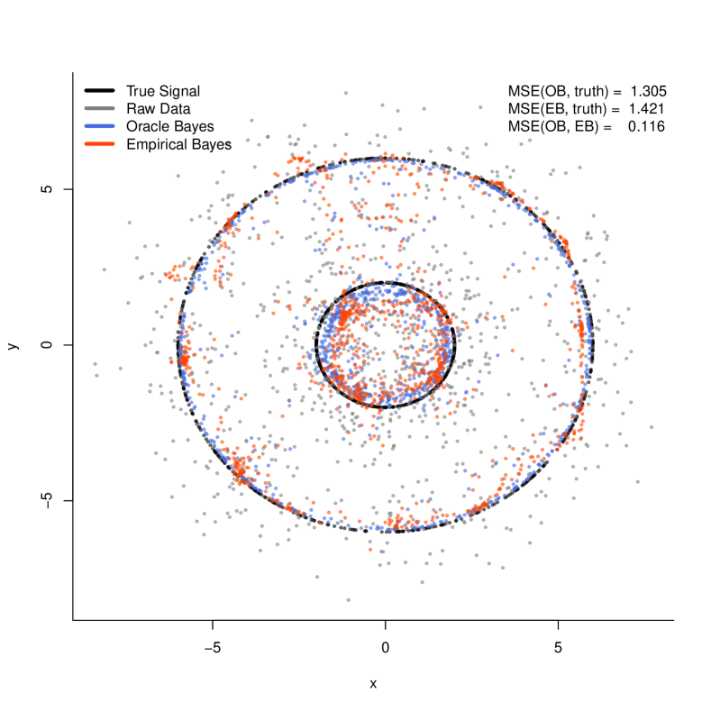
(a) Two circles: $n=1000$. Half of $\{\theta_{i}\}_{i=1}^{n}$ are drawn uniformly at random from each of the concentric circles of radii $2$ and $6$ respectively.

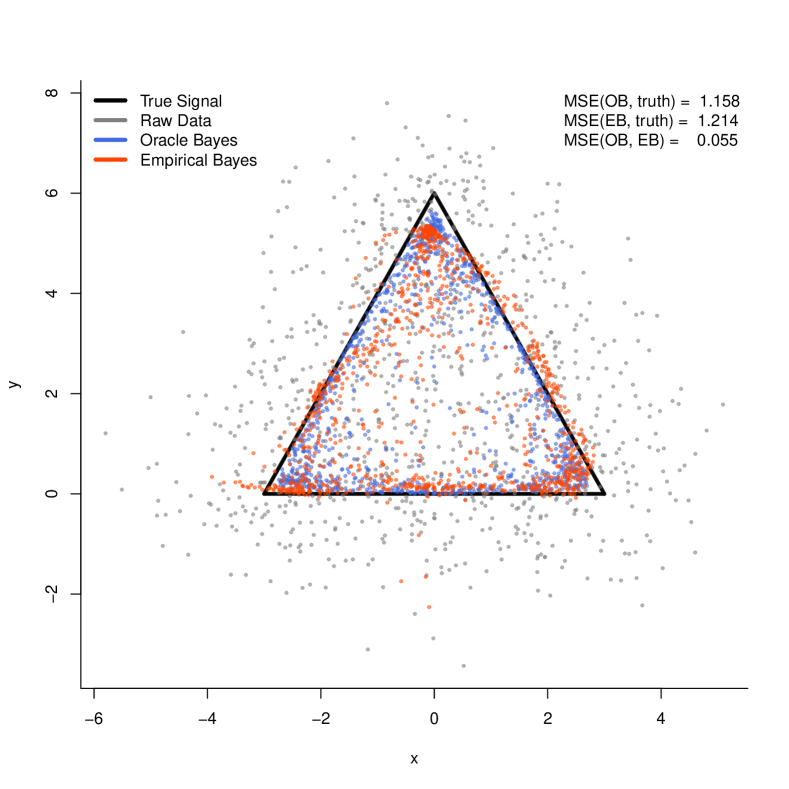
(b) Triangle: $n=999$. A third of $\{\theta_{i}\}_{i=1}^{n}$ are drawn uniformly at random from each edge of the triangle with vertices $(-3,0)$, $(0,6)$ and $(3,0)$

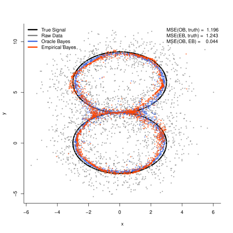
(c) Digit $8$: $n=1000$. Half of $\{\theta_{i}\}_{i=1}^{n}$ are drawn uniformly at random from each of the circles of radii $3$ cnetered at $(0,0)$ and $(0,6)$ respectively.

(d) Letter A: $n=1000$. A fifth of $\{\theta_{i}\}_{i=1}^{n}$ are drawn uniformly at random from each of the line segments joining the points $(-4,-6),(-2,0),(0,6),(2,0)$ and $(4,6)$ so as to form the letter A.

Figure 1: Illustrations of denoising using the Empirical Bayes estimates (1.7)

In each of the four subfigures in Figure 1, we generate $n$ vectors $\theta_{1},\dots,\theta_{n}$ from a bounded region in ${\mathbb{R}}^{d}$ for $d=2$: they are generated from two concentric circles in the first subfigure, a triangle in the second subfigure, the digit 8 in the third subfigure and the uppercase letter A in the last subfigure. In each of these cases, the empirical measure $\bar{G}_{n}$ is supported on a bounded region so that Corollary 3.2 yields the near parametric rate $1/n$ up to logarithmic multiplicative factors in $n$ for every NPMLE. In each of the subfigures in Figure 1, we plot the true parameter values $\theta_{1},\dots,\theta_{n}$ in black, the data $X_{1},\dots,X_{n}$ (generated independently according to $X_{i}\sim N(\theta_{i},I_{2})$) are plotted in gray, the Oracle Bayes estimates $\hat{\theta}_{1}^{*},\dots,\hat{\theta}_{n}^{*}$ are plotted in blue while the estimates $\hat{\theta}_{1},\dots,\hat{\theta}_{n}$ are plotted in red. The mean squared discrepancies:

$$\frac{1}{n}\sum_{i=1}^{n}\left\lVert\hat{\theta}_{i}^{*}-\theta_{i}\right\rVert^{2},~{}~{}~{}\frac{1}{n}\sum_{i=1}^{n}\left\lVert\hat{\theta}_{i}-\theta_{i}\right\rVert^{2}\text{ and }~{}~{}~{}\frac{1}{n}\sum_{i=1}^{n}\left\lVert\hat{\theta}_{i}^{*}-\hat{\theta}_{i}\right\rVert^{2}$$

are given in each figure in the legend at the upper-right corner. Note that the third MSE is much smaller than the other two in each subfigure.

As can be observed from Figure 1, the Empirical Bayes estimates (1.7) approximate their targets (1.6) quite well. The most noteworthy fact is that the estimates (1.7) do not require any knowlege of the underlying structure in $\bar{G}_{n}$, for instance, concentric circles, or triangle or a letter of the alphabet etc. We should also note here that the noise distribution here is completely known to be $N(0,I_{d})$ which implies, in particular, that there is no unknown scale parameter representing the noise variance.

We have also done numerical simulations for illustrating the denoising performance of $\hat{\theta}_{1},\dots,\hat{\theta}_{n}$ in the case when $\theta_{1},\dots,\theta_{n}$ have a clustering structure. Due to space constraints, these results have been moved to Section G of the technical appendix.

This technical appendix contains proofs of all results in the main paper. Some observations on the heteroscedastic Gaussian denoising problem are also given in this appendix. The proofs for results in Section 2 are given in Section A while the proofs for Section 3 are in Section B. Section C contains some results and remarks on the heteroscedastic problem. Metric entropy results for multivariate Gaussian location mixture densities play a crucial rule in the proofs of the main results; these results are stated and proved in Section D. Section E contains the statement and proof for a crucial ingredient for the proof of the main denoising theorem. Finally, additional technical results needed in the proofs of the main results are collected in Section F together with their proofs while additional simulation results are in Section G. .

Appendix A Proofs of results in Section 2

The following notation will be used in the proofs in the sequel.

1. For $x\in{\mathbb{R}}^{d}$ and $a>0$, let $B(x,a):=\{u\in{\mathbb{R}}^{d}:\|u-x\|\leq a\}$ denote the closed ball of radius $a$ centered at $x$.

2. For a subset $S\subseteq{\mathbb{R}}^{d}$ and $a>0$, we denote the set $S^{a}$ by

$$S^{a}:=\cup_{x\in S}B(x,a)=\left\{y:{\mathfrak{d}_{S}}(y)\leq a\right\}$$ (A.1)

where ${\mathfrak{d}_{S}}(\cdot)$ is defined as in (2.1).

3. For a compact subset $S$ of ${\mathbb{R}}^{d}$ and $\epsilon>0$, we denote the $\epsilon$-covering number of $S$ in the usual Euclidean distance by $N(\epsilon,S)$ i.e., $N(\epsilon,S)$ stands for the smallest number of closed balls of radius $\epsilon$ whose union contains $S$.

4. Given a pseudometric $\varrho$ on ${\mathcal{M}}$, let $N(\epsilon,{\mathcal{M}},\varrho)$ denote the $\epsilon$-covering number of ${\mathcal{M}}$ under the pseudometric $\varrho$ by $N(\epsilon,{\mathcal{M}},\varrho)$ i.e., $N(\epsilon,{\mathcal{M}},\varrho)$ denotes the smallest positive integer $N$ for which there exist densities $f_{1},\dots,f_{N}\in{\mathcal{M}}$ satisfying

$$\sup_{f\in{\mathcal{M}}}\inf_{1\leq i\leq N}\varrho(f,f_{i})\leq\epsilon.$$

In the proof below, we will be concerned with $N(\epsilon,{\mathcal{M}},\varrho)$ for the following choice of $\varrho$. For a compact set $S$, let $\left\lVert\cdot\right\rVert_{\infty,S}$ denote the pseudonorm on ${\mathcal{M}}$ defined by

$$\|f\|_{\infty,S}:=\sup_{x\in S}|f(x)|.$$ (A.2)

This pseudonorm naturally induces a pseudometric on ${\mathcal{M}}$ given by $\varrho(f,g):=\left\lVert f-g\right\rVert_{\infty,S}$. The covering number for this pseudometric will be denoted by $N(\epsilon,{\mathcal{M}},\left\lVert\cdot\right\rVert_{\infty,S})$. In the proofs for the results in Section 3, we will need to deal with covering numbers for other pseudometrics $\varrho$ on ${\mathcal{M}}$ as well. These pseudometrics will be introduced in Section B.

With the above notation in place, we are now ready to give the proof of Theorem 2.1. This proof uses additional ingredients which are proved in later sections. Arguably the most important ingredient for the proof of this theorem is a bound on the covering numbers $N(\epsilon,{\mathcal{M}},\left\lVert\cdot\right\rVert_{\infty,S})$ which is stated as inequality (4.1) in Theorem 4.1. Other ingredients include inequality (F.11) (which is a consequence of Lemma 4.2) and a standard fact (Lemma F.6) giving a volumetric upper bound for Euclidean covering numbers.

A.1 Proof of Theorem 2.1

Proof of Theorem 2.1.

We shall prove inequalities (2.5) and (2.6) under the assumption that the sample size $n$ satisfies

$$n\geq\max\left(\exp\left(\frac{d+1}{2}\right),\frac{1}{2}(2\pi)^{(d-1)/2}\right).$$ (A.3)

If (A.3) is not satisfied, then $\epsilon_{n}(M,S,\bar{G}_{n})$ (and $\epsilon_{n}(M,S,\bar{G}_{n})/\min(1-\alpha,\beta)$ which is larger than $\epsilon_{n}(M,S,\bar{G}_{n})$) will be bounded from below by a positive constant $\kappa_{d}$. We can then therefore choose $C_{d}$ in (2.5) and (2.6) large enough so that $\epsilon_{n}(M,S,\bar{G}_{n})\sqrt{C_{d}}>\sqrt{2\min(1-\alpha,\beta)}$. Because the Hellinger distance ${\mathfrak{H}}(\hat{f}_{n},f_{\bar{G}_{n}})$ is always bounded from above by $\sqrt{2}$, the probability on the left hand side of (2.5) will then equal zero so that (2.5) holds trivially. Inequality (2.6) will also be trivial because its right hand side will then be larger than 2.

Let us therefore fix $n$ satisfying (A.3). Fix a positive sequence $\{\gamma_{n}\}$ and assume that $\hat{f}_{n}$ satisfies

$$\prod_{i=1}^{n}\frac{\hat{f}_{n}(X_{i})}{f_{\bar{G}_{n}}(X_{i})}\geq\exp\left((\beta-\alpha)n\gamma_{n}^{2}\right)\qquad\text{for some $0<\beta\leq\alpha<1$}.$$ (A.4)

We shall then bound the probability

$${\mathbb{P}}\{{\mathfrak{H}}(\hat{f}_{n},f_{\bar{G}_{n}})\geq t\gamma_{n}\}\qquad\text{for $t\geq 1$}.$$

Fix a non-empty compact set $S\subseteq{\mathbb{R}}^{d}$ and $M\geq\sqrt{10\log n}$. We shall work with the set $S^{M}$ (defined as in (A.1)) and the pseudometric given by the pseudonorm $\left\lVert\cdot\right\rVert_{\infty,S^{M}}$ (defined as in (A.2)).

Let $\eta:=1/n^{2}$ and let $\{h_{1},\dots,h_{N}\}\subseteq{\mathcal{M}}$ denote an $\eta$-covering set of ${\mathcal{M}}$ in the pseudometric given by $\|\cdot\|_{\infty,S^{M}}$ where $N=N(\eta,{\mathcal{M}},\|\cdot\|_{\infty,S^{M}})$ i.e.,

$$\sup_{h\in{\mathcal{M}}}\inf_{1\leq j\leq N}\|h-h_{j}\|_{\infty,S^{M}}\leq\eta.$$

Inequality (4.1) in Theorem 4.1 gives an upper bound for $N$ that will be crucially used in this proof.

Let $J$ denote the set of all $j\in\{1,\dots,N\}$ for which there exists a density $h_{0j}\in{\mathcal{M}}$ satisfying

$$\|h_{0j}-h_{j}\|_{\infty,S^{M}}\leq\eta~{}~{}\text{ and }~{}~{}{\mathfrak{H}}(h_{0j},f_{\bar{G}_{n}})\geq t\gamma_{n}.$$

Because $h_{1},\dots,h_{N}$ cover ${\mathcal{M}}$, there will exist $1\leq j\leq N$ such that $\|h_{j}-\hat{f}_{n}\|_{\infty,S^{M}}\leq\eta$. If ${\mathfrak{H}}(\hat{f}_{n},f_{\bar{G}_{n}})\geq t\gamma_{n}$, then $j\in J$ and consequently

$$\|\hat{f}_{n}-h_{0j}\|_{\infty,S^{M}}\leq 2\eta.$$ (A.5)

We now define a function $v:=v_{S,M}:{\mathbb{R}}^{d}\rightarrow(0,\infty)$ via

$$v(x):=\begin{cases}\eta&\text{ if }x\in S^{M}\\ \eta\left(\frac{M}{\mathfrak{d}_{S}(x)}\right)^{d+1}&\text{ otherwise }\end{cases}$$ (A.6)

where $\mathfrak{d}_{S}:{\mathbb{R}}^{d}\rightarrow[0,\infty)$ is defined as in (2.1).

Inequality (A.5) clearly implies that $\hat{f}_{n}(X_{i})\leq h_{0j}(X_{i})+2\eta=h_{0j}(X_{i})+2v(X_{i})$ whenever $X_{i}\in S^{M}$ which allows us to write

$$\prod_{i=1}^{n}\hat{f}_{n}(X_{i})\leq\prod_{i:X_{i}\in S^{M}}\left\{h_{0j}(X_{i})+2v(X_{i})\right\}\prod_{i:X_{i}\notin S^{M}}(2\pi)^{-d/2}$$

where we used the bound $\hat{f}_{n}(X_{i})\leq\sup_{x}\hat{f}_{n}(x)\leq(2\pi)^{-d/2}$ for $X_{i}\notin S^{M}$ (the bound $\sup_{x}f(x)\leq(2\pi)^{-d/2}$ holds for every $f\in{\mathcal{M}}$ as can easily be seen). From here, we deduce

$$\prod_{i=1}^{n}\hat{f}_{n}(X_{i}) \leq\prod_{i=1}^{n}\left\{h_{0j}(X_{i})+2v(X_{i})\right\}\prod_{i:X_{i}\notin S^{M}}\frac{(2\pi)^{-d/2}}{h_{0j}(X_{i})+2v(X_{i})}$$

$$\leq\prod_{i=1}^{n}\left\{h_{0j}(X_{i})+2v(X_{i})\right\}\prod_{i:X_{i}\notin S^{M}}\frac{(2\pi)^{-d/2}}{2v(X_{i})}$$

We have therefore proved that the inequality

$$\prod_{i=1}^{n}\frac{\hat{f}_{n}(X_{i})}{f_{\bar{G}_{n}}(X_{i})}\leq\max_{j\in J}\prod_{i=1}^{n}\frac{h_{0j}(X_{i})+2v(X_{i})}{f_{\bar{G}_{n}}(X_{i})}\prod_{i:X_{i}\notin S^{M}}\frac{(2\pi)^{-d/2}}{2v(X_{i})}$$

holds on the event ${\mathfrak{H}}(\hat{f}_{n},f_{\bar{G}_{n}})\geq t\gamma_{n}$. Because $\hat{f}_{n}$ satisfies (A.4), we obtain

$${\mathbb{P}}\left({\mathfrak{H}}(\hat{f}_{n},f_{\bar{G}_{n}})\geq t\gamma_{n}\right) \leq{\mathbb{P}}\bigg{\{}\max_{j\in J}\prod_{i=1}^{n}\frac{h_{0j}(X_{i})+2v(X_{i})}{f_{\bar{G}_{n}}(X_{i})}\prod_{i:X_{i}\notin S^{M}}\frac{(2\pi)^{-d/2}}{2v(X_{i})}$$

$$\geq\exp\left((\beta-\alpha)nt^{2}\gamma_{n}^{2}\right)\bigg{\}}$$

$$\leq{\mathbb{P}}\bigg{\{}\max_{j\in J}\prod_{i=1}^{n}\frac{h_{0j}(X_{i})+2v(X_{i})}{f_{\bar{G}_{n}}(X_{i})}\geq e^{-\alpha nt^{2}\gamma_{n}^{2}}\bigg{\}}$$ (A.7)

$$+{\mathbb{P}}\bigg{\{}\prod_{i:X_{i}\notin S^{M}}\frac{(2\pi)^{-d/2}}{2v(X_{i})}\geq e^{\beta nt^{2}\gamma_{n}^{2}}\bigg{\}}.$$

We shall bound the two probabilities above separately. For the first probability:

$$P_{\textup{I}}:={\mathbb{P}}\left\{\max_{j\in J}\prod_{i=1}^{n}\frac{h_{0j}(X_{i})+2v(X_{i})}{f_{\bar{G}_{n}}(X_{i})}\geq e^{-\alpha nt^{2}\gamma_{n}^{2}}\right\},$$

we write

$$P_{\textup{I}} \leq\sum_{j\in J}{\mathbb{P}}\left\{\prod_{i=1}^{n}\frac{h_{0j}(X_{i})+2v(X_{i})}{f_{\bar{G}_{n}}(X_{i})}\geq e^{-\alpha nt^{2}\gamma_{n}^{2}}\right\}$$

$$\leq e^{\alpha nt^{2}\gamma_{n}^{2}/2}\sum_{j\in J}{\mathbb{E}}\prod_{i=1}^{n}\sqrt{\frac{h_{0j}(X_{i})+2v(X_{i})}{f_{\bar{G}_{n}}(X_{i})}}$$

$$=e^{\alpha nt^{2}\gamma_{n}^{2}/2}\sum_{j\in J}\prod_{i=1}^{n}{\mathbb{E}}\sqrt{\frac{h_{0j}(X_{i})+2v(X_{i})}{f_{\bar{G}_{n}}(X_{i})}}.$$

Now for each fixed $j\in J$, we have

$$\prod_{i=1}^{n}{\mathbb{E}}\sqrt{\frac{h_{0j}(X_{i})+2v(X_{i})}{f_{\bar{G}_{n}}(X_{i})}} =\exp\left(\sum_{i=1}^{n}\log{\mathbb{E}}\sqrt{\frac{h_{0j}(X_{i})+2v(X_{i})}{f_{\bar{G}_{n}}(X_{i})}}\right)$$

$$\leq\exp\left(\sum_{i=1}^{n}{\mathbb{E}}\sqrt{\frac{h_{0j}(X_{i})+2v(X_{i})}{f_{\bar{G}_{n}}(X_{i})}}-n\right)$$

$$\leq\exp\left(\sum_{i=1}^{n}\int\sqrt{\frac{h_{0j}+2v}{f_{\bar{G}_{n}}}}f_{G_{i}}-n\right)$$

$$=\exp\left(n\int\sqrt{\left(h_{0j}+2v\right)f_{\bar{G}_{n}}}-n\right).$$

Because of $\sqrt{\alpha+\beta}\leq\sqrt{\alpha}+\sqrt{\beta}$ and the Cauchy-Schwarz inequality (along with $\int f_{\bar{G}_{n}}=1$), we obtain

$$\int\sqrt{\left(h_{0j}+2v\right)f_{\bar{G}_{n}}} \leq\int\sqrt{h_{0j}f_{\bar{G}_{n}}}+\sqrt{2}\int\sqrt{vf_{\bar{G}_{n}}}$$

$$\leq\int\sqrt{h_{0j}f_{\bar{G}_{n}}}+\sqrt{2}\sqrt{\int v}$$

$$=1-\frac{1}{2}{\mathfrak{H}}^{2}(h_{0j},f_{\bar{G}_{n}})+\sqrt{2}\sqrt{\int v}.$$

We now use Lemma F.5 which gives an upper bound on $\int v$. This (along with the fact that ${\mathfrak{H}}(h_{0j},f_{\bar{G}_{n}})\geq t\gamma_{n}$) allows us to deduce:

$$\int\sqrt{\left(h_{0j}+2v(X_{i})\right)f_{\bar{G}_{n}}}\leq 1-\frac{t^{2}}{2}\gamma_{n}^{2}+C_{d}\sqrt{2\eta\text{Vol}(S^{M})}.$$

We have therefore proved that

$$P_{\textup{I}} \leq\exp\left(\frac{\alpha}{2}nt^{2}\gamma^{2}_{n}+\log|J|-\frac{1}{2}nt^{2}\gamma_{n}^{2}+nC_{d}\sqrt{\eta\text{Vol}(S^{M})}\right)$$

$$\leq\exp\left(\frac{\alpha-1}{2}nt^{2}\gamma_{n}^{2}+\log N+C_{d}\sqrt{\text{Vol}(S^{M})}\right)$$ (A.8)

because $\eta:=n^{-2}$ and $|J|\leq N$ (as $J\subseteq\{1,\dots,N\}$).

We now use the upper bound on $N$ from inequality (4.1) in Theorem 4.1. Because $\eta=1/n^{2}$ and $n\geq 2$, the quantity $a$ appearing in Theorem 4.1 satisfies

$$a=\sqrt{2\log\frac{2\sqrt{2\pi}}{(2\pi)^{d/2}\eta}}=\sqrt{2\log\frac{2\sqrt{2\pi}}{(2\pi)^{d/2}}+4\log n}\leq\sqrt{6\log n}.$$

Also because of (A.3), we have $2n\geq(2\pi)^{(d-1)/2}$ so that

$$a=\sqrt{2\log\frac{2\sqrt{2\pi}}{(2\pi)^{d/2}\eta}} =\sqrt{2\log\frac{2\sqrt{2\pi}}{(2\pi)^{d/2}}+4\log n}$$

$$\geq\sqrt{2\log(1/n)+4\log n}=\sqrt{2\log n}.$$

Thus Theorem 4.1 gives

$$\log N\leq C_{d}N(a,(S^{M})^{a})(\log n)^{d+1}\leq C_{d}N(\sqrt{2\log n},S^{M+\sqrt{6\log n}})(\log n)^{d+1}.$$

Using Lemma F.6 to bound the Euclidean covering number appearing in the right hand side above, we deduce that

$$N(\sqrt{2\log n},S^{M+\sqrt{6\log n}}) \leq C_{d}(\sqrt{2\log n})^{-d}\text{Vol}(S^{M+\sqrt{6\log n}+\sqrt{2\log n}/2})$$

$$\leq C_{d}(\log n)^{-d/2}\text{Vol}(S^{M+\sqrt{10\log n}})$$

$$\leq C_{d}(\log n)^{-d/2}\text{Vol}(S^{2M})$$

as $M\geq\sqrt{10\log n}$. This gives $\log N\leq C_{d}(\log n)^{(d/2)+1}\text{Vol}(S^{2M})$. Using this bound for $\log N$ in (A.8), we obtain

$$P_{\textup{I}} \leq\exp\bigg{(}\frac{\alpha-1}{2}nt^{2}\gamma_{n}^{2}+C_{d}(\log n)^{(d/2)+1}\text{Vol}(S^{2M})+C_{d}\sqrt{\text{Vol}(S^{M})}\bigg{)}.$$

We shall now bound the second probability in (A.7):

$$P_{\textup{II}}:={\mathbb{P}}\left\{\prod_{i:X_{i}\notin S^{M}}\frac{(2\pi)^{-d/2}}{2v(X_{i})}\geq e^{\beta nt^{2}\gamma_{n}^{2}}\right\}.$$

First observe, by Markov’s inequality, that

$$P_{\textup{II}}\leq\exp\left(-\frac{\beta nt^{2}\gamma_{n}^{2}}{2\log n}\right){\mathbb{E}}\left(\prod_{i:X_{i}\notin S^{M}}\frac{(2\pi)^{-d/2}}{2v(X_{i})}\right)^{1/(2\log n)}$$

The expectation above is bounded as (recall the formula for $v(\cdot)$ from (A.6))

$${\mathbb{E}}\left(\prod_{i:X_{i}\notin S^{M}}\frac{(2\pi)^{-d/2}}{2v(X_{i})}\right)^{\frac{1}{2\log n}} \leq{\mathbb{E}}\left(\prod_{i:X_{i}\notin S^{M}}\frac{1}{v(X_{i})}\right)^{\frac{1}{2\log n}}$$

$$={\mathbb{E}}\left(\prod_{i:X_{i}\notin S^{M}}\frac{\mathfrak{d}_{S}(X_{i})}{M\eta^{\frac{1}{d+1}}}\right)^{\frac{d+1}{2\log n}}$$

$$={\mathbb{E}}\left[\prod_{i=1}^{n}\left(\frac{\mathfrak{d}_{S}(X_{i})}{M\eta^{\frac{1}{d+1}}}\right)^{I\{\mathfrak{d}_{S}(X_{i})\geq M\}}\right]^{\frac{d+1}{2\log n}}$$

The above term will be controlled below by using inequality (F.11) (which is a consequence of Lemma 4.2) with

$$a:=\frac{1}{M\eta^{1/(d+1)}}~{}~{}~{}~{}~{}\text{ and }~{}~{}~{}~{}~{}\lambda:=\frac{d+1}{2\log n}$$ (A.9)

to obtain

$${\mathbb{E}}\left[\prod_{i=1}^{n}\left(\frac{\mathfrak{d}_{S}(X_{i})}{M\eta^{\frac{1}{d+1}}}\right)^{I\{\mathfrak{d}_{S}(X_{i})\geq M\}}\right]^{\frac{d+1}{2\log n}} \leq\exp\bigg{\{}C_{d}a^{\lambda}M^{\lambda+d-2}$$ (A.10)

$$+(aM)^{\lambda}n\left(\frac{2\mu_{p}(\mathfrak{d}_{S},\bar{G}_{n})}{M}\right)^{p}\bigg{\}}.$$

We need to assume here that

$$\log n\geq\frac{d+1}{2\min(1,p)}$$

to ensure that $\lambda\leq\min(1,p)$ as required for inequality (F.11). This is satisfied as long as $p\geq(d+1)/(2\log n)$ because under the assumption (A.3), we have $\log n\geq\frac{d+1}{2}$. Thus (A.10) holds for all $p\geq(d+1)/(2\log n)$.

For notational convenience, we write $\mu_{p}:=\mu_{p}(\mathfrak{d}_{S},\bar{G}_{n})$ in the rest of the proof. With the choices (A.9) (and $\eta=1/n^{2}$), the first term in the exponent of the right hand side of (A.10) is calculated as

$$a^{\lambda}M^{\lambda+d-2}=M^{d-2}\eta^{-\lambda/(d+1)}=M^{d-2}n^{1/(\log n)}=eM^{d-2}.$$

On the other hand, the second term in the exponent in (A.10) becomes

$$(aM)^{\lambda}n\left(\frac{2\mu_{p}(\mathfrak{d}_{S},\bar{G}_{n})}{M}\right)^{p}=en\left(\frac{2\mu_{p}}{M}\right)^{p}.$$

Therefore the second probability in (A.7) satisfies the inequality:

$$P_{\textup{II}}\leq\exp\left(-\frac{\beta nt^{2}\gamma_{n}^{2}}{2\log n}+C_{d}M^{d-2}+en\left(\frac{2\mu_{p}}{M}\right)^{p}\right).$$

This is true for all $p\geq(d+1)/(2\log n)$ so we can also write

$$P_{\textup{II}}\leq\exp\left(-\frac{\beta nt^{2}\gamma_{n}^{2}}{2\log n}+C_{d}M^{d-2}+en\inf_{p\geq(d+1)/(2\log n)}\left(\frac{2\mu_{p}}{M}\right)^{p}\right).$$

We have proved therefore that for every $t>0$

$${\mathbb{P}}\left\{{\mathfrak{H}}(\hat{f}_{n},f_{\bar{G}_{n}})\geq t\gamma_{n}\right\} \leq\exp\left(\frac{\alpha-1}{2}nt^{2}\gamma_{n}^{2}+C_{d}(\log n)^{(d/2)+1}\text{Vol}(S^{2M})\right.$$

$$\left.+C_{d}\sqrt{\text{Vol}(S^{M})}\right)+\exp\left(-\frac{\beta nt^{2}\gamma_{n}^{2}}{2\log n}+C_{d}M^{d-2}\right.$$

$$\left.+en\inf_{p\geq(d+1)/(2\log n)}\left(\frac{2\mu_{p}}{M}\right)^{p}\right).$$

We now note that ${\mathrm{Vol}}(S^{M})\leq{\mathrm{Vol}}(S^{2M})\leq C_{d}M^{d}{\mathrm{Vol}}(S^{1})$ which follows from inequality (F.25) in Lemma F.6. This, along with the definition of $\epsilon^{2}_{n}(M,S,\bar{G}_{n})$ in (2.3), gives that

$$\max\left((\log n)^{\frac{d}{2}+1}{\mathrm{Vol}}(S^{2M}),\sqrt{{\mathrm{Vol}}(S^{M})},M^{d},n(\log n)\inf_{p\geq\frac{d+1}{2\log n}}\left(\frac{2\mu_{p}}{M}\right)^{p}\right)$$

is bounded from above by $C_{d}n\epsilon_{n}^{2}(M,S,\bar{G}_{n})$. As a result,

$${\mathbb{P}}\left\{{\mathfrak{H}}(\hat{f}_{n},f_{\bar{G}_{n}})\geq t\gamma_{n}\right\} \leq\exp\left(\frac{\alpha-1}{2}nt^{2}\gamma_{n}^{2}+C_{d}n\epsilon_{n}^{2}(M,S,\bar{G}_{n})\right)$$

$$+\exp\left(-\frac{\beta nt^{2}\gamma_{n}^{2}}{2\log n}+C_{d}\frac{n\epsilon_{n}^{2}(M,S,\bar{G}_{n})}{\log n}\right).$$

Now suppose that

$$\gamma_{n}^{2}=C_{d}^{\prime}\frac{\epsilon^{2}_{n}(M,S,\bar{G}_{n})}{\min(1-\alpha,\beta)}$$ (A.11)

for some $C_{d}^{\prime}\geq 4C_{d}$. We deduce then that, for every $t\geq 1$,

$${\mathbb{P}}\left\{{\mathfrak{H}}(\hat{f}_{n},f_{\bar{G}_{n}})\geq t\gamma_{n}\right\} \leq\exp\left(-\frac{1-\alpha}{2}nt^{2}\gamma_{n}^{2}+\frac{1-\alpha}{4}n\gamma_{n}^{2}\right)$$

$$+\exp\left(-\frac{\beta}{2\log n}nt^{2}\gamma_{n}^{2}+\frac{\beta}{4\log n}n\gamma_{n}^{2}\right)$$

$$\leq 2\exp\left(-\frac{\min((1-\alpha),\beta)}{4\log n}nt^{2}\gamma_{n}^{2}\right)$$ (A.12)

Observe now that (because $M\geq\sqrt{10\log n}$)

$$\epsilon_{n}^{2}(M,S,\bar{G}_{n})\geq{\mathrm{Vol}}(S^{1})\frac{M^{d}}{n}\left(\sqrt{\log n}\right)^{d+2}\geq{\mathrm{Vol}}(B(0,1))\frac{(\log n)^{2}}{n}$$

so that we can choose the constant $C_{d}^{\prime}$ such that

$$n\min(1-\alpha,\beta)\gamma_{n}^{2}\geq C_{d}^{\prime}n\epsilon_{n}^{2}(M,S,\bar{G}_{n})\geq 4(\log n)^{2}.$$

This gives, via (A.12),

$${\mathbb{P}}\left\{{\mathfrak{H}}(\hat{f}_{n},f_{\bar{G}_{n}})\geq t\gamma_{n}\right\}\leq 2n^{-t^{2}}.$$

We have therefore proved the above inequality for $\gamma_{n}$ as chosen in (A.11) (provided $C_{d}^{\prime}$ is chosen sufficiently large) for every estimator $\hat{f}_{n}$ satisfying (A.4). This completes the proof of (2.5).

For (2.6), we multiply both sides of (2.5) by $t$ and then integrate from $t=1$ to $t=\infty$ to obtain

$${\mathbb{E}}\bigg{(}\frac{{\mathfrak{H}}^{2}(\hat{f}_{n},f_{\bar{G}_{n}})\min(1-\alpha,\beta)}{C_{d}\epsilon_{n}^{2}(M,S,\bar{G}_{n})}\bigg{)}\leq 1+4\int_{1}^{\infty}tn^{-t^{2}}\leq 1+\frac{2}{n\log n}\leq 4$$

which proves (2.6) and completes the proof of Theorem 2.1. ∎

A.2 Proof of Corollary 2.2

Proof of Corollary 2.2.

To prove (2.7), assume that $\bar{G}_{n}$ is supported on a compact set $S$. We then apply Theorem 2.1 to this $S$ and $M=\sqrt{10\log n}$. Because $\bar{G}_{n}$ is supported on $S$, we have $\mu_{p}({\mathfrak{d}_{S}},\bar{G}_{n})=0$ for every $p>0$ so that $\epsilon_{n}^{2}(M,S,\bar{G}_{n})$ (defined in (2.3)) becomes

$$\epsilon_{n}^{2}(M,S,\bar{G}_{n})={\mathrm{Vol}}(S^{1})\frac{M^{d}}{n}\left(\sqrt{\log n}\right)^{d+2}=(10)^{d/2}\frac{{\mathrm{Vol}}(S^{1})}{n}\left(\log n\right)^{d+1}.$$

Inequality (2.7) then immediately follows from Theorem 2.1.

We next prove (2.9) assuming the condition (2.8). Let

$$M:=4K(e\log n)^{1/\alpha}.$$ (A.13)

This quantity $M\geq\sqrt{10\log n}$ because $K\geq 1$ and $\alpha\leq 2$. We shall apply (2.6) with this $M$. Let

$$T_{2}(M,S,\bar{G}_{n}):=(\log n)\inf_{p\geq\frac{d+1}{2\log n}}\bigg{(}\frac{2\mu_{p}({\mathfrak{d}_{S}},\bar{G}_{n})}{M}\bigg{)}^{p}$$

and note that this is the second term on the right hand side of (2.3) in the definition of $\epsilon_{n}^{2}(M,S,\bar{G}_{n})$. The infimum over $p$ above is easily seen to be achieved at $p=(M/(2K))^{\alpha}(1/e)$. By the expression (A.13) for $M$, it is easy to see that $p\geq(d+1)/(2\log n)$ provided

$$n\geq\exp\left(\sqrt{(d+1)/2}\right).$$ (A.14)

We then deduce that

$$T_{2}(M,S,\bar{G}_{n})\leq(\log n)\exp\left(\frac{-1}{\alpha e}\left(\frac{M}{2K}\right)^{\alpha}\right).$$

It follows from here that $T_{2}(M,S,\bar{G}_{n})\leq(\log n)/n$ because $M\geq(4K)(e\log n)^{1/\alpha}\geq(2K)(\alpha e\log n)^{1/\alpha}$. Thus

$$\epsilon^{2}_{n}(M,S,\bar{G}_{n}) ={\mathrm{Vol}}(S^{1})\frac{M^{d}}{n}\left(\sqrt{\log n}\right)^{d+2}+T_{2}(M,S,\bar{G}_{n})$$

$$\leq{\mathrm{Vol}}(S^{1})\frac{(4Ke^{1/\alpha})^{d}}{n}(\log n)^{d/\alpha}\left(\sqrt{\log n}\right)^{d+2}+\frac{\log n}{n}$$ (A.15)

and hence (2.9) readily follows as a consequence of Theorem 2.1. When the assumption (A.14) does not hold, inequality (2.9) becomes trivially true when $C_{d}$ is chosen sufficiently large.

We now turn to (2.10). Assume that $S$ is such that $\mu_{p}({\mathfrak{d}_{S}},\bar{G}_{n})\leq\mu$ for fixed $\mu>0$ and $p>0$. Then Theorem 2.1 gives

$${\mathbb{E}}{\mathfrak{H}}^{2}(\hat{f}_{n},f_{\bar{G}_{n}}) \leq C_{d}\inf_{M\geq\sqrt{10\log n}}\epsilon_{n}^{2}(M,S,\bar{G}_{n})$$

$$=C_{d}\inf_{M\geq\sqrt{10\log n}}\left(\mathrm{Vol}(S^{1})\frac{M^{d}}{n}\left(\sqrt{\log n}\right)^{d+2}\right.$$

$$\left.+\left(\log n\right)\left(\frac{2\mu}{M}\right)^{p}\right)$$

where we assumed that $n$ is large enough so that $p\geq(d+1)/(2\log n)$. Taking

$$M=\left(\sqrt{\log n}\right)^{-d/(p+d)}\left(\frac{n\mu^{p}}{{\mathrm{Vol}}(S^{1})}\right)^{1/(p+d)}$$

results in (2.10). When $n$ is large enough, $M$ chosen as above exceeds $\sqrt{10\log n}$. For smaller $n$, the inequality (2.10) trivially holds provided $C_{d,\mu,p}$ is chosen large enough. ∎

A.3 Proof of Lemma 2.4

The following uses standard ideas involving Assouad’s lemma (see, for example, Tsybakov [58, Chapter 2].

Proof of Lemma 2.4.

Fix $\delta>0$ and $M>0$. Let $a_{1},\dots,a_{k}$ and $b_{1},\dots,b_{k}$ be points in ${\mathbb{R}}^{d}$ such that

$$\min\bigg{(}\min_{i\neq j}\left\lVert a_{i}-a_{j}\right\rVert,\min_{i\neq j}\left\lVert b_{i}-b_{j}\right\rVert,\min_{i\neq j}\left\lVert a_{i}-b_{j}\right\rVert\bigg{)}\geq M$$ (A.16)

and such that

$$\left\lVert a_{i}-b_{i}\right\rVert=\delta\qquad\text{for every $1\leq i\leq k$}.$$ (A.17)

Now for every $\tau\in\{0,1\}^{k}$, let

$$f_{\tau}(x)=\frac{1}{k}\sum_{i=1}^{k}\phi_{d}(x-a_{i}(1-\tau_{i})-b_{i}\tau_{i})$$

where $\phi_{d}(\cdot)$ is the standard normal density on ${\mathbb{R}}^{d}$. Clearly $f_{\tau}\in{\mathcal{M}}_{k}$ for every $\tau\in\{0,1\}^{k}$. We shall now employ Assouad’s lemma which gives

$${\mathcal{R}}({\mathcal{M}}_{k})\geq\frac{k}{8}\min_{\tau\neq\tau^{\prime}}\frac{{\mathfrak{H}}^{2}(f_{\tau},f_{\tau^{\prime}})}{\Upsilon(\tau,\tau^{\prime})}\min_{\Upsilon(\tau,\tau^{\prime})=1}\bigg{(}1-\left\lVert P_{f_{\tau}}-P_{f_{\tau^{\prime}}}\right\rVert_{TV}\bigg{)}$$

where $\Upsilon(\tau,\tau^{\prime}):=\sum_{i=1}^{k}I\{\tau_{j}\neq\tau_{j}^{\prime}\}$ denotes Hamming distance and $P_{f}$ (for $f\in{\mathcal{M}}$) denotes the joint distribution of $X_{1},\dots,X_{n}$ which are independently distributed according to $f$.

We now fix $\tau\neq\tau^{\prime}\in\{0,1\}^{k}$ and bound ${\mathfrak{H}}^{2}(f_{\tau},f_{\tau^{\prime}})$ from below. For simplicity, let $f=f_{\tau}$ and $g=f_{\tau^{\prime}}$. Also, for $i=1,\dots,k$, let

$$f_{i}(x):=\phi_{d}(x-a_{i}(1-\tau_{i})-b_{i}\tau_{i})~{}~{}\text{ and }~{}~{}g_{i}(x):=\phi_{d}(x-a_{i}(1-\tau_{i}^{\prime})-b_{i}\tau_{i}^{\prime})$$

so that $f=\sum_{i=1}^{k}f_{i}/k$ and $g=\sum_{i=1}^{k}g_{i}/k$. This gives

$$\frac{1}{2}{\mathfrak{H}}^{2}(f,g) =1-\int\sqrt{f(x)g(x)}dx$$

$$=1-\int\sqrt{\frac{1}{k^{2}}\sum_{i,j}f_{i}(x)g_{j}(x)}dx\geq 1-\frac{1}{k}\sum_{i,j}\int\sqrt{f_{i}(x)g_{j}(x)}dx.$$

Because $f_{i}$ and $g_{j}$ are normal densities, by a straightforward computation, we obtain

$$\int\sqrt{f_{i}(x)g_{j}(x)}dx=\exp\left(-\left\lVert a_{i}(1-\tau_{i})+b_{i}\tau_{i}-a_{j}(1-\tau_{j}^{\prime})-b_{j}\tau_{j}^{\prime}\right\rVert^{2}/8\right)$$

so that by (A.16) and (A.17), we obtain that

$$\int\sqrt{f_{i}(x)g_{j}(x)}dx=I\{\tau_{i}=\tau_{i}^{\prime}\}+I\{\tau_{i}\neq\tau_{i}^{\prime}\}e^{-\delta^{2}/8}\qquad\text{for $i=j$}$$

and

$$\int\sqrt{f_{i}(x)g_{j}(x)}dx\leq e^{-M^{2}/8}\qquad\text{for $i\neq j$}.$$

As a result, we obtain

$$\frac{1}{2}{\mathfrak{H}}^{2}(f_{\tau},f_{\tau^{\prime}}) =1-\frac{1}{k}\sum_{i=1}^{k}\int\sqrt{f_{i}(x)g_{i}(x)}dx-\frac{1}{k}\sum_{i\neq j}\int\sqrt{f_{i}(x)g_{j}(x)}dx$$

$$\geq 1-\frac{1}{k}\sum_{i=1}^{k}I\{\tau_{i}=\tau_{i}^{\prime}\}-\frac{e^{-\delta^{2}/8}}{k}\Upsilon(\tau,\tau^{\prime})-\frac{k^{2}-k}{k}e^{-M^{2}/8}$$

$$=\frac{1}{k}\Upsilon(\tau,\tau^{\prime})\left(1-e^{-\delta^{2}/8}\right)-(k-1)e^{-M^{2}/8}$$ (A.18)

for every $\tau\neq\tau^{\prime}\in\{0,1\}^{k}$. Now let us fix $\tau,\tau^{\prime}$ with $\Upsilon(\tau,\tau^{\prime})=1$ and bound from above the total variation distance between $P_{f_{\tau}}$ and $P_{f_{\tau^{\prime}}}$. Without loss of generality, we can assume that $\tau_{1}\neq\tau_{1}^{\prime}$ and that $\tau_{i}=\tau_{i}^{\prime}$ for $i\geq 2$. Below $D(P_{f_{\tau}}||P_{f_{\tau^{\prime}}})$ denotes the Kullback-Leibler divergence between $P_{f_{\tau}}$ and $P_{f_{\tau^{\prime}}}$. Also $D(f_{\tau}||f_{\tau^{\prime}})$ and $\chi^{2}(f_{\tau},f_{\tau^{\prime}})$ denote the Kullback-Leibler divergence and chi-squared divergence between the densities $f_{\tau}$ and $f_{\tau^{\prime}}$ respectively. By Pinsker’s inequality and the fact that $D(f_{\tau}||f_{\tau^{\prime}})\leq\chi^{2}(f_{\tau},f_{\tau^{\prime}})$, we obtain

$$\left\lVert P_{f_{\tau}}-P_{f_{\tau^{\prime}}}\right\rVert_{TV}\leq\sqrt{\frac{1}{2}D(P_{f_{\tau}}||P_{f_{\tau^{\prime}}})}=\sqrt{\frac{n}{2}D({f_{\tau}}||{f_{\tau^{\prime}}})}\leq\sqrt{\frac{n}{2}\chi^{2}({f_{\tau}}||{f_{\tau^{\prime}}})}.$$

Further

$$\chi^{2}({f_{\tau}}||{f_{\tau^{\prime}}}) =\int\frac{(f_{\tau}(x)-f_{\tau^{\prime}}(x))^{2}}{f_{\tau^{\prime}}(x)}dx$$

$$=\int\frac{\left(\phi_{d}(x-a_{1}(1-\tau_{1})-b_{1}\tau_{1})-\phi_{d}(x-a_{1}(1-\tau_{1}^{\prime})-b_{1}\tau_{1}^{\prime})\right)^{2}}{k^{2}f_{\tau^{\prime}}(x)}dx$$

$$\leq\int\frac{\left(\phi_{d}(x-a_{1}(1-\tau_{1})-b_{1}\tau_{1})-\phi_{d}(x-a_{1}(1-\tau_{1}^{\prime})-b_{1}\tau_{1}^{\prime})\right)^{2}}{k\phi_{d}(x-a_{1}(1-\tau_{1}^{\prime})-b_{1}\tau_{1}^{\prime})}dx.$$

By a routine calculation, it now follows that

$$\chi^{2}(f_{\tau}||f_{\tau^{\prime}}) \leq\frac{1}{k}\left\{\exp\left(\left\lVert a_{1}(1-\tau_{1})+b_{1}\tau_{1}-a_{1}(1-\tau_{1}^{\prime})-b_{1}\tau_{1}^{\prime}\right\rVert^{2}\right)-1\right\}$$

$$=\frac{1}{k}\left\{\exp\left(\left\lVert a_{1}-b_{1}\right\rVert^{2}\right)-1\right\}=\frac{1}{k}\left(e^{\delta^{2}}-1\right).$$

We have therefore proved that

$$\left\lVert P_{f_{\tau}}-P_{f_{\tau^{\prime}}}\right\rVert_{TV}\leq\sqrt{\frac{n}{2k}\left(e^{\delta^{2}}-1\right)}$$ (A.19)

for every $\tau,\tau^{\prime}\in\{0,1\}^{k}$ with $\Upsilon(\tau,\tau^{\prime})=1$. Combining (A.18) and (A.19), we obtain

$${\mathcal{R}}({\mathcal{M}}_{k})\geq\frac{k}{4}\left(\frac{1}{k}\left(1-e^{-\delta^{2}/8}\right)-\frac{(k-1)}{\Upsilon(\tau,\tau^{\prime})}e^{-M^{2}/8}\right)\left(1-\sqrt{\frac{n}{2k}\left(e^{\delta^{2}}-1\right)}\right).$$

This inequality holds for every $\delta>0$ and $M>0$. So we can let $M$ tend to $\infty$ to deduce

$${\mathcal{R}}({\mathcal{M}}_{k})\geq\frac{1}{4}\left(1-e^{-\delta^{2}/8}\right)\left(1-\sqrt{\frac{n}{2k}\left(e^{\delta^{2}}-1\right)}\right)$$

for every $\delta>0$. The inequalities $1-e^{-t}\geq t/2$ and $e^{t}-1\leq 2t$ for $0\leq t\leq 1$ imply that

$${\mathcal{R}}({\mathcal{M}}_{k})\geq\frac{\delta^{2}}{64}\left(1-\sqrt{\frac{n}{k}}\delta\right)\qquad\text{for every $0\leq\delta\leq 1$}.$$

The choice $\delta=\sqrt{k/4n}$ now proves (2.13). ∎

A.4 Proof of Theorem 2.5

Proof of Theorem 2.5.

Note that

$$h^{*}(x)=\sum_{j=1}^{k}w_{j}\phi_{d}(x;\mu_{j},\Sigma_{j})=\sum_{j=1}^{k}w_{j}\det(\Sigma_{j}^{-1/2})\phi_{d}\left(\Sigma_{j}^{-1/2}(x-\mu_{j})\right)$$

where $\phi_{d}(z):=(2\pi)^{-d/2}\exp\left(-\left\lVert z\right\rVert^{2}/2\right)$ denotes the standard $d$-dimensional normal density. It is then easy to see that $X_{1},\dots,X_{n}$ (where $X_{i}=Y_{i}/\sigma_{\min}$) are independent observations having the density $f^{*}$ where

$$f^{*}(x) =\sigma_{\min}^{d}h^{*}(\sigma_{\min}x)$$

$$=\sum_{j=1}^{k}w_{j}\left[\det\left(\sigma_{\min}^{-2}\Sigma_{j}\right)^{-1/2}\right]\phi_{d}\left(\left\{\sigma^{-2}_{\min}\Sigma_{j}\right\}^{-1}\left(x-\sigma^{-1}_{\min}\mu_{j}\right)\right).$$

This means that $f^{*}$ is the density of the normal mixture:

$$\sum_{j=1}^{k}w_{j}N\left(\sigma_{\min}^{-1}\mu_{j},\sigma_{\min}^{-2}\Sigma_{j}\right)$$

where $N(\mu,\Sigma)$ denotes the multivariate normal distribution with mean vector $\mu$ and covariance matrix $\Sigma$. It follows from here that $f^{*}$ equals $f_{G^{*}}$ (in the notation (1.1)) where $G^{*}$ is the distribution of the normal mixture

$$\sum_{j=1}^{k}w_{j}N\left(\sigma_{\min}^{-1}\mu_{j},\sigma_{\min}^{-2}\Sigma_{j}-I_{d}\right)$$

where $I_{d}$ is the $d\times d$ identity matrix.

We can now use Corollary 2.2 to bound ${\mathfrak{H}}^{2}(\hat{f}_{n},f^{*})$ (note that $\hat{f}_{n}$ is an NPMLE based on $X_{1},\dots,X_{n}$). Specifically we shall use inequality (2.9) with

$$S:=\left\{\sigma_{\min}^{-1}\mu_{1},\dots,\sigma_{\min}^{-1}\mu_{k}\right\}.$$

In order to verify (2.8), observe first that $\bar{G}_{n}$ in Corollary 2.2 is $G^{*}$ since $X_{1},\dots,X_{n}$ are i.i.d $f_{G^{*}}$ and that

$${\mathfrak{d}_{S}}(\theta)=\min_{1\leq i\leq k}\left\lVert\sigma_{\min}^{-1}\mu_{i}-\theta\right\rVert$$

As a result, for every $p\geq 1$ and $Z\sim N(0,I_{d})$, we have

$$\mu_{p}({\mathfrak{d}_{S}},\bar{G}_{n}) \leq\left({\mathbb{E}}\max_{1\leq j\leq k}\left\lVert\left(\sigma_{\min}^{-2}\Sigma_{j}-I_{d}\right)^{1/2}Z\right\rVert^{p}\right)^{1/p}$$

$$\leq\sqrt{\frac{\sigma_{\max}^{2}}{\sigma_{\min}^{2}}-1}\left({\mathbb{E}}\left\lVert Z\right\rVert^{p}\right)^{1/p}\leq C_{d}\tau\sqrt{p}.$$

Thus (2.8) holds with $K:=C_{d}\max(1,\tau)$ and $\alpha=2$ and inequality (2.9) then gives

$${\mathbb{E}}{\mathfrak{H}}^{2}(\hat{f}_{n},f^{*})\leq C_{d}\frac{{\mathrm{Vol}}(S^{1})}{n}\left(\max(1,\tau)\right)^{d}(\log n)^{d+1}$$

As $S$ is a finite set of cardinality $k$, we have ${\mathrm{Vol}}(S^{1})\leq kC_{d}$ so that

$${\mathbb{E}}{\mathfrak{H}}^{2}(\hat{f}_{n},f^{*})\leq C_{d}\left(\frac{k}{n}\right)\left(\max(1,\tau)\right)^{d}(\log n)^{d+1}.$$

We now use the fact that the Hellinger distance is invariant under scale transformations which implies that ${\mathfrak{H}}(\hat{f}_{n},f^{*})={\mathfrak{H}}(\hat{h}_{n},h^{*})$. This proves inequality (2.17). ∎

Appendix B Proofs of Results in Section 3

B.1 Proof of Theorem 3.1

Theorem 3.1 is a special of Theorem 3.5 (indeed, taking $\Sigma_{i}=I_{d}$ for each $i$ in Theorem 3.5 leads to Theorem 3.1). Therefore, the proof of Theorem 3.1 follows from the proof of Theorem 3.5 which is given in Subsection B.5.

B.2 Proof of Corollary 3.2

The idea is to choose $M$ and $S$ appropriately under each of the assumptions on $\bar{G}_{n}$ and then to appropriately bound $\epsilon_{n}(M,S)$. The necessary work for this is already done in Corollary 2.2 from which Corollary 3.2 immediately follows.

B.3 Proof of Proposition 3.3

The assumption (3.5) implies that the empirical measure $\bar{G}_{n}$ of $\theta_{1},\dots,\theta_{n}$ is supported on

$$S:=\cup_{j=1}^{k}B(a_{j},R)\qquad\text{where $B(a_{j},R):=\left\{x\in{\mathbb{R}}^{d}:\left\lVert x-a_{j}\right\rVert\leq R\right\}$}.$$

We can therefore apply inequality (3.2) in Corollary 3.2 to bound ${\mathfrak{R}}_{n}(\hat{\theta},\hat{\theta}^{*})$. The conclusion (3.6) then immediately follows from (3.2) because

$${\mathrm{Vol}}(S^{1})\leq\sum_{j=1}^{k}{\mathrm{Vol}}(B(a_{j},1+R))\leq C_{d}k(1+R)^{d}.$$

B.4 Proof of Lemma 3.4

The proof of Lemma 3.4 uses Assouad’s lemma (see, for example, Tsybakov [58, Chapter 2] as well as Lemma F.8 (stated and proved in Section F).

Proof of Lemma 3.4.

Fix $k$ and $n$ with $1\leq k\leq n$. Also fix $\delta>0$ and $M\geq 2$. Let $a_{1},\dots,a_{k}$ and $b_{1},\dots,b_{k}$ be points in ${\mathbb{R}}^{d}$ such that

$$\min\left(\min_{i\neq j}\left\lVert a_{i}-a_{j}\right\rVert,\min_{i\neq j}\left\lVert b_{i}-b_{j}\right\rVert,\min_{i\neq j}\left\lVert a_{i}-b_{j}\right\rVert\right)\geq M$$ (B.1)

and such that

$$\left\lVert a_{i}-b_{i}\right\rVert=\delta\qquad\text{for every $1\leq i\leq k$}.$$ (B.2)

We now define a partition $S_{1},\dots,S_{k},S_{k+1}$ of $\{1,\dots,n\}$ via

$$S_{i}:=\left\{(i-1)m+1,\dots,im\right\}\qquad\text{for $i=1,\dots,k$}$$

and $S_{k+1}:=\{km+1,\dots,n\}$ where $m:=[n/k]$ ( for $x>0$, we define $[x]$ as usual to be the largest integer that is smaller than or equal to $x$). Note that the cardinality of $S_{j}$ equals $m$ for $i=1,\dots,k$ and that $S_{k+1}$ will be empty if $n$ is a multiple of $k$.

Now for every $\tau\in\{0,1\}^{k}$, we define $n$ vectors $\theta_{1}(\tau),\dots,\theta_{n}(\tau)$ in ${\mathbb{R}}^{d}$ via

$$\theta_{i}(\tau):=(1-\tau_{j})a_{j}+\tau_{j}b_{j}\qquad\text{provided $i\in S_{j}$ for some $1\leq j\leq k$}$$

and for $i\in S_{k+1}$, we take $\theta_{i}(\tau):=a_{1}$.

Let $\Theta(\tau)$ denote the collection of all $n$-tuples $(\theta_{1}(\tau),\dots,\theta_{n}(\tau))$ as $\tau$ ranges over $\{0,1\}^{k}$. It is easy to see that $\Theta(\tau)\subseteq\Theta_{n,d,k}$ so that

$${\mathcal{R}}^{*}(\Theta_{n,d,k})\geq{\mathcal{R}}^{*}(\Theta(\tau)):=\inf_{\tilde{\theta}_{1},\dots,\tilde{\theta}_{n}}\sup_{(\theta_{1},\dots,\theta_{n})\in\Theta(\tau)}{\mathbb{E}}\left[\frac{1}{n}\sum_{i=1}^{n}\left\lVert\tilde{\theta}_{i}-\hat{\theta}_{i}^{*}\right\rVert^{2}\right].$$

The elementary inequality $\left\lVert a-b\right\rVert^{2}\geq\left\lVert a\right\rVert^{2}/2-\left\lVert b\right\rVert^{2}$ for vectors $a,b\in{\mathbb{R}}^{d}$ gives

$$\frac{1}{n}\sum_{i=1}^{n}\left\lVert\tilde{\theta}_{i}-\hat{\theta}_{i}^{*}\right\rVert^{2}\geq\frac{1}{2n}\sum_{i=1}^{n}\left\lVert\tilde{\theta}_{i}-\theta_{i}\right\rVert^{2}-\frac{1}{n}\sum_{i=1}^{n}\left\lVert\hat{\theta}_{i}^{*}-\theta_{i}\right\rVert^{2}$$

for every $\theta_{1},\dots,\theta_{n}$ and estimators $\tilde{\theta}_{1}\dots,\tilde{\theta}_{n}$. As a result, we deduce that

$${\mathcal{R}}^{*}(\Theta(\tau))\geq\breve{{\mathcal{R}}}(\Theta(\tau))-\sup_{(\theta_{1},\dots,\theta_{n})\in\Theta(\tau)}{\mathbb{E}}\left[\frac{1}{n}\sum_{i=1}^{n}\left\lVert\hat{\theta}_{i}^{*}-\theta_{i}\right\rVert^{2}\right]$$ (B.3)

where

$$\breve{{\mathcal{R}}}(\Theta(\tau)):=\inf_{\tilde{\theta}_{1},\dots,\tilde{\theta}_{n}}\sup_{(\theta_{1},\dots,\theta_{n})\in\Theta(\tau)}{\mathbb{E}}\left[\frac{1}{n}\sum_{i=1}^{n}\left\lVert\tilde{\theta}_{i}-\theta_{i}\right\rVert^{2}\right].$$

We first bound $\breve{{\mathcal{R}}}(\Theta(\tau))$ from below via Assouad’s lemma. For $\tau,\tau^{\prime}\in\{0,1\}^{k}$, let

$${\mathfrak{L}}(\tau,\tau^{\prime}):=\frac{1}{n}\sum_{i=1}^{n}\left\lVert\theta_{i}(\tau)-\theta_{i}(\tau^{\prime})\right\rVert^{2}.$$

Also let $P_{\tau}$ denote the joint distribution of the independent random variables $X_{1},\dots,X_{n}$ with $X_{i}\sim N(\theta_{i}(\tau),I_{d})$ for $i=1,\dots,n$. Assouad’s lemma then gives

$$\breve{{\mathcal{R}}}(\Theta(\tau))\geq\frac{k}{8}\min_{\tau\neq\tau^{\prime}}\frac{{\mathfrak{L}}(\tau,\tau^{\prime})}{\Upsilon(\tau,\tau^{\prime})}\min_{\Upsilon(\tau,\tau^{\prime})=1}\left(1-\left\lVert P_{\tau}-P_{\tau^{\prime}}\right\rVert_{TV}\right)$$ (B.4)

where $\Upsilon(\tau,\tau^{\prime}):=\sum_{j=1}^{k}I\{\tau_{j}\neq\tau_{j}^{\prime}\}$ is the Hamming distance and $\left\lVert P_{\tau}-P_{\tau^{\prime}}\right\rVert_{TV}$ denotes the variation distance between $P_{\tau}$ and $P_{\tau^{\prime}}$. We now bound the terms appearing in the right hand side of (B.4). For $\tau,\tau^{\prime}\in\{0,1\}^{k}$, observe that

$${\mathfrak{L}}(\tau,\tau^{\prime}) =\frac{1}{n}\sum_{j=1}^{k}\sum_{i:i\in S_{j}}\left\lVert a_{j}-b_{j}\right\rVert^{2}I\{\tau_{j}\neq\tau^{\prime}_{j}\}$$

$$=\frac{1}{n}\sum_{j=1}^{k}|S_{j}|\left\lVert a_{j}-b_{j}\right\rVert^{2}I\{\tau_{j}\neq\tau^{\prime}_{j}\}=\frac{m\delta^{2}}{n}\Upsilon(\tau,\tau^{\prime})$$ (B.5)

where $|S_{j}|$ denotes the cardinality of $S_{j}$. We have used above the fact that $|S_{j}|=m$ for $1\leq j\leq k$ and (B.2).

To bound the last term in (B.4), we use Pinsker’s inequality (below $D$ stands for Kullback-Leibler divergence) to obtain

$$\left\lVert P_{\tau}-P_{\tau^{\prime}}\right\rVert_{TV}\leq\sqrt{\frac{1}{2}D(P_{\tau}||P_{\tau^{\prime}})}=\frac{1}{2}\sqrt{\sum_{i=1}^{n}\left\lVert\theta_{i}(\tau)-\theta_{i}(\tau^{\prime})\right\rVert^{2}}=\frac{1}{2}\sqrt{n{\mathfrak{L}}(\tau,\tau^{\prime})}.$$

Thus, from (B.5), we deduce that for $\Upsilon(\tau,\tau^{\prime})=1$,

$$\left\lVert P_{\tau}-P_{\tau^{\prime}}\right\rVert_{TV}\leq\frac{1}{2}\sqrt{m\delta^{2}}.$$

Inequality (B.4) thus gives

$$\breve{{\mathcal{R}}}(\Theta(\tau))\geq\frac{km\delta^{2}}{8n}\left(1-\frac{\sqrt{m\delta^{2}}}{2}\right).$$ (B.6)

To bound the second term in (B.3), we use Lemma F.8 which gives that for every $\theta_{1},\dots,\theta_{n}\in\Theta(\tau)$, we have

$${\mathbb{E}}\left[\frac{1}{n}\sum_{i=1}^{n}\left\lVert\hat{\theta}_{i}^{*}-\theta_{i}\right\rVert^{2}\right]\leq\frac{k}{2\sqrt{2\pi}}\sum_{j,l:j\neq l}\left(p_{j}+p_{l}\right)\left\lVert c_{j}-c_{l}\right\rVert\exp\left(-\frac{1}{8}\left\lVert c_{j}-c_{l}\right\rVert^{2}\right)$$

where $c_{1},\dots,c_{k+1}$ denote the distinct elements from $\theta_{1},\dots,\theta_{n}$ and $p_{j},j=1,\dots,k+1$ are nonnegative real numbers summing to one. Now each $c_{j}$ equals either $a_{j}$ or $b_{j}$ and hence, by (B.1), we have $\left\lVert c_{j}-c_{l}\right\rVert\geq M$ for every $j\neq l$. As $x\mapsto xe^{-x^{2}/8}$ is decreasing for $x>2$ and $M>2$, we deduce that

$${\mathbb{E}}\left[\frac{1}{n}\sum_{i=1}^{n}\left\lVert\hat{\theta}_{i}^{*}-\theta_{i}\right\rVert^{2}\right]\leq\frac{k}{2\sqrt{2\pi}}Me^{-M^{2}/8}\sum_{j,l:j\neq l}\left(p_{j}+p_{l}\right)\leq\frac{k}{\sqrt{2\pi}}Me^{-M^{2}/8}.$$ (B.7)

We obtain therefore from (B.3), (B.6) and (B.7), that

$${\mathcal{R}}^{*}(\Theta_{n,d,k})\geq\frac{km\delta^{2}}{8n}\left(1-\frac{\sqrt{m\delta^{2}}}{2}\right)-\frac{k}{\sqrt{2\pi}}Me^{-M^{2}/8}.$$

The left hand side above does not depend on $M$ so we can let $M\rightarrow\infty$ to obtain

$${\mathcal{R}}^{*}(\Theta_{n,d,k})\geq\frac{km\delta^{2}}{8n}\left(1-\frac{\sqrt{m\delta^{2}}}{2}\right).$$

We now make the choice $\delta:=1/\sqrt{m}$ to obtain ${\mathcal{R}}^{*}(\Theta_{n,d,k})\geq k/(16n)$ which proves Lemma 3.4. ∎

B.5 Proof of Theorem 3.5

The proof of Theorem 3.5 is similar to Jiang and Zhang [27, Proof of Theorem 5]. It uses ingredients that are proved in Section D, Section E and Section F. More precisely, crucial roles are played by the metric entropy results of Section D (specifically Corollary D.1) and Theorem E.1 in Section E which relates the denoising error to Hellinger distance (thereby allowing the application of Theorem 2.1). Additionally, Lemma 4.2 and Lemma 4.3 from Section 4 as well as Lemma F.1, Lemma F.3 and Lemma F.6 from Section F will also be used.

Basically, the following proof bounds ${\mathfrak{R}}_{n}(\hat{\theta},\hat{\theta}^{*})$ in terms of five quantities $\zeta_{1n}^{2},\dots,\zeta_{5n}^{2}$. The additional $(\log n)^{\max(d,3)}$ factor in Theorem 3.5 (compared to Theorem 2.1) comes from the bounds used for the terms involving $\zeta_{4n}^{2}$ and $\zeta_{5n}^{2}$.

The notation described at the beginning of Section A will be followed in this section as well.

Proof of Theorem 3.5.

The goal is to bound

$${\mathfrak{R}}_{n}(\hat{\theta},\breve{\theta}^{*}) ={\mathbb{E}}\left(\frac{1}{n}\sum_{i=1}^{n}\|\hat{\theta}_{i}-\breve{\theta}_{i}^{*}\|^{2}\right)$$

$$={\mathbb{E}}\left(\frac{1}{n}\sum_{i=1}^{n}\left\lVert X_{i}+\frac{\nabla\hat{f}_{n}(X_{i})}{\hat{f}_{n}(X_{i})}-X_{i}-\frac{\nabla f_{\bar{G}^{0}_{n}}(X_{i})}{f_{\bar{G}^{0}_{n}}(X_{i})}\right\rVert^{2}\right)$$

Let us now introduce the following notation. Let ${\mathbf{X}}$ denote the $d\times n$ matrix whose columns are the observed data vectors $X_{1},\dots,X_{n}$. For a density $f\in{\mathcal{M}}$, let $T_{f}({\mathbf{X}})$ denote the $d\times n$ matrix whose $i^{th}$ column is given by the $d\times 1$ vector:

$$X_{i}+\frac{\nabla f(X_{i})}{f(X_{i})}\qquad\text{for $i=1,\dots,n$}.$$

With this notation, we can clearly rewrite ${\mathfrak{R}}_{n}(\hat{\theta},\hat{\theta}^{*})$ as

$${\mathfrak{R}}_{n}(\hat{\theta},\breve{\theta}^{*})={\mathbb{E}}\left(\frac{1}{n}\left\lVert T_{\hat{f}_{n}}({\mathbf{X}})-T_{f_{\bar{G}^{0}_{n}}}({\mathbf{X}})\right\rVert_{F}^{2}\right)$$

where $\left\lVert\cdot\right\rVert_{F}$ denotes the usual Frobenius norm for matrices.

To bound the above, we first observe that since $\hat{f}_{n}$ is an NPMLE defined as in (1.2), it follows from the general maximum likelihood theorem (see, for example, Böhning [7, Theorem 2.1]) that

$$\frac{1}{n}\sum_{i=1}^{n}\frac{\phi_{d}(X_{i}-\theta)}{\hat{f}_{n}(X_{i})}\leq 1$$ (B.8)

for every $\theta\in{\mathbb{R}}^{d}$. Taking $\theta=X_{i}$ in the above inequality, we deduce that

$$1\geq\frac{\phi_{d}(X_{i}-\theta)}{n\hat{f}_{n}(X_{i})}=\frac{\phi_{d}(0)}{n\hat{f}_{n}(X_{i})}$$

so that $\hat{f}_{n}(X_{i})\geq\phi_{d}(0)/n=(2\pi)^{-d/2}n^{-1}$. Since this is true for each $i=1,\dots,n$, this means that

$$\min_{1\leq i\leq n}\hat{f}_{n}(X_{i})\geq\rho_{n}:=\frac{(2\pi)^{-d/2}}{n}.$$ (B.9)

As a result, $\hat{f}_{n}(X_{i})=\max(\hat{f}_{n}(X_{i}),\rho_{n})$ for each $i$ so that $T_{\hat{f}_{n}}({\mathbf{X}})=T_{\hat{f}_{n}}({\mathbf{X}},\rho_{n})$ where for $f\in{\mathcal{M}}$ and $\rho>0$, we define $T_{f}({\mathbf{X}},\rho)$ to be the $d\times n$ matrix whose $i^{th}$ column is given by the $d\times 1$ vector:

$$X_{i}+\frac{\nabla f(X_{i})}{\max(f(X_{i}),\rho)}\qquad\text{for $i=1,\dots,n$}.$$

This gives

$${\mathfrak{R}}_{n}(\hat{\theta},\hat{\theta}^{*})={\mathbb{E}}\left(\frac{1}{n}\left\lVert T_{\hat{f}_{n}}({\mathbf{X}},\rho_{n})-T_{f_{\bar{G}^{0}_{n}}}({\mathbf{X}})\right\rVert_{F}^{2}\right).$$

A difficulty in dealing with the expectation on the right hand side above comes from the fact that $\hat{f}_{n}$ is random. This is handled by covering the random $\hat{f}_{n}$ by an $\epsilon$-net for a specific $\epsilon$ in the following way. First fix a compact set $S\subseteq{\mathbb{R}}^{d}$ and $M\geq\sqrt{10\log n}$. Note that by Theorem 2.1 (specifically inequality (2.5) applied to $\alpha=\beta=0.5$ and $t=1$), we deduce that the following inequality holds with probability at least $1-(2/n)$:

$${\mathfrak{H}}(\hat{f}_{n},f_{\bar{G}_{n}^{0}})\leq\tilde{C}_{d}\epsilon_{n}(M,S,\bar{G}_{n}^{0}).$$ (B.10)

Here $\tilde{C}_{d}$ is a positive constant depending on $d$ alone and $\epsilon_{n}(M,S,\bar{G}^{0}_{n})$ is defined as in (2.3). Note that Theorem 2.1 is indeed applicable here as $X_{1},\dots,X_{n}$ are independent random vectors with

$$X_{i}\sim N(\theta_{i},\Sigma_{i})=f_{G_{i}^{0}}$$

where $G_{i}^{0}$ is the $N(\theta_{i},\Sigma_{i}-I_{d})$ and $\bar{G}^{0}_{n}$ is the average of $G_{i}^{0}$ over $i=1\dots,n$.

Let $E_{n}$ denote the event that (B.10) holds. We now obtain a covering of

$$\{f\in{\mathcal{M}}:{\mathfrak{H}}(f,f_{\bar{G}^{0}_{n}})\leq\tilde{C}_{d}\epsilon_{n}(M,S,\bar{G}_{n}^{0})\}$$ (B.11)

under the pseudometric given by

$$\left\lVert f-g\right\rVert_{S^{M},\nabla}^{\rho_{n}}:=\sup_{x\in S^{M}}\left\lVert\frac{\nabla f(x)}{\max(f(x),\rho_{n})}-\frac{\nabla g(x)}{\max(g(x),\rho_{n})}\right\rVert$$ (B.12)

where $S^{M}:=\{x\in{\mathbb{R}}^{d}:{\mathfrak{d}_{S}}(x)\leq M\}$. We have proved covering number bounds under this pseudometric in Corollary D.1 which will be used in this proof. Let $f_{G_{1}},\dots,f_{G_{N}}$ denote a maximal subset of (B.11) such that for every $i\neq j$, we have

$$\left\lVert f_{G_{i}}-f_{G_{j}}\right\rVert_{S^{M},\nabla}^{\rho_{n}}\geq 2\eta^{*}$$ (B.13)

where $\eta^{*}$ is defined in terms of

$$\eta^{*}:=\left(\frac{1}{\rho_{n}}+\sqrt{\frac{1}{\rho_{n}^{2}}\log\frac{1}{(2\pi)^{d}\rho_{n}^{2}}}\right)\eta~{}~{}~{}\text{ and }~{}~{}~{}\eta:=\frac{\rho_{n}}{n}.$$ (B.14)

By the usual relation between packing and covering numbers, the integer $N$ is then bounded from above by $N(\eta^{*},{\mathcal{M}},\left\lVert\cdot\right\rVert_{S^{M}N,\nabla}^{\rho_{n}})$ which is bounded in Corollary D.1. Specifically, Corollary D.1 (applied to $S^{M}$) gives

$$\log N\leq C_{d}N(a,(S^{M})^{a})|\log\eta|^{d+1}\leq C_{d}N(a,S^{M+a})(\log n)^{d+1}$$

where

$$a:=\sqrt{2\log(2\sqrt{2\pi}n^{2})}.$$ (B.15)

This further implies (via the use of inequality (F.24) in Lemma F.6 to bound $N(a,S^{M+a})$ as $N(a,S^{M+a})\leq C_{d}a^{-d}{\mathrm{Vol}}(S^{M+(3a/2)})$) that

$$\log N\leq C_{d}(\log n)^{d+1}a^{-d}{\mathrm{Vol}}(S^{M+(3a/2)})\leq C_{d}(\log n)^{(d/2)+1}{\mathrm{Vol}}(S^{M+(3a/2)}).$$

Using (F.25) in Lemma F.6 to bound ${\mathrm{Vol}}(S^{M+(3a/2)})$ in terms of ${\mathrm{Vol}}(S^{1})$ (and the fact that $a\leq C\sqrt{10\log n}\leq CM$), we obtain

$$\log N\leq C_{d}{\mathrm{Vol}}(S^{1})M^{d}(\log n)^{(d/2)+1}.$$ (B.16)

Also because $f_{G_{1}},\dots,f_{G_{N}}$ is a maximal subset of (B.11) satisfying (B.13), we have

$$\max_{1\leq j\leq N}{\mathfrak{H}}(f_{G_{j}},f_{\bar{G}^{0}_{n}})\leq\tilde{C}_{d}\epsilon_{n}(M,S,\bar{G}_{n}^{0})$$ (B.17)

and, on the event $E_{n}$,

$$\min_{1\leq j\leq N}\left\lVert\hat{f}_{n}-f_{G_{j}}\right\rVert_{S^{M},\nabla}^{\rho_{n}}\leq 2\eta^{*}.$$ (B.18)

We are now ready to bound the risk ${\mathfrak{R}}_{n}(\hat{\theta},\breve{\theta}^{*})$. The strategy is to break down the risk into various terms involving the densities $f_{G_{1}},\dots,f_{G_{N}}$.

Breakdown of the risk: The risk

$${\mathfrak{R}}_{n}(\hat{\theta},\breve{\theta}^{*})={\mathbb{E}}\left(\frac{1}{n}\left\lVert T_{\hat{f}_{n}}({\mathbf{X}},\rho_{n})-T_{f_{\bar{G}^{0}_{n}}}({\mathbf{X}})\right\rVert_{F}^{2}\right)$$

will be broken down via the inequality:

$$\|T_{\hat{f}_{n}}(\mathbf{X},\rho_{n})-T_{f_{\bar{G}_{n}^{0}}}(\mathbf{X})\|_{F} \leq\|T_{\hat{f}_{n}}(\mathbf{X},\rho_{n})-T_{f_{\bar{G}^{0}_{n}}}(\mathbf{X},\rho_{n})\|_{F}$$ (B.19)

$$+\|T_{f_{\bar{G}^{0}_{n}}}(\mathbf{X},\rho_{n})-T_{f_{\bar{G}^{0}_{n}}}(\mathbf{X})\|_{F}$$

$$\leq(\zeta_{1n}+\zeta_{2n}+\zeta_{3n}+\zeta_{4n})+\zeta_{5n}$$ (B.20)

where

$$\zeta_{1n} :=\|T_{\hat{f}_{n}}(\mathbf{X},\rho_{n})-T_{f_{\bar{G}^{0}_{n}}}(\mathbf{X},\rho_{n})\|_{F}I(E^{c}_{n})$$

$$\zeta_{2n} :=\left(\|T_{\hat{f}_{n}}(\mathbf{X},\rho_{n})-T_{f_{\bar{G}^{0}_{n}}}(\mathbf{X},\rho_{n})\|_{F}\right.$$

$$\left.-\max_{1\leq j\leq N}\|T_{f_{G_{j}}}(\mathbf{X},\rho_{n})-T_{f_{\bar{G}^{0}_{n}}}(\mathbf{X},\rho_{n})\|_{F}\right)_{+}I(E_{n})$$

$$\zeta_{3n} :=\max_{1\leq j\leq N}\left(\|T_{f_{G_{j}}}(\mathbf{X},\rho_{n})-T_{f_{\bar{G}_{n}^{0}}}(\mathbf{X},\rho_{n})\|_{F}\right.$$

$$\left.-{\mathbb{E}}\|T_{f_{G_{j}}}(\mathbf{X},\rho_{n})-T_{f_{\bar{G}^{0}_{n}}}(\mathbf{X},\rho_{n})\|_{F}\right)_{+}$$

$$\zeta_{4n} :=\max_{1\leq j\leq N}{\mathbb{E}}\|T_{f_{G_{j}}}(\mathbf{X},\rho_{n})-T_{f_{\bar{G}^{0}_{n}}}(\mathbf{X},\rho_{n})\|_{F}$$

$$\zeta_{5n} :=\|T_{f_{\bar{G}^{0}_{n}}}(\mathbf{X})-T_{f_{\bar{G}^{0}_{n}}}(\mathbf{X},\rho_{n})\|_{F}$$

With the elementary inequality $(a_{1}+\dots+a_{5})^{2}\leq 5(a_{1}^{2}+\dots+a_{5}^{2})$, inequality (B.20) gives

$${\mathfrak{R}}_{n}(\hat{\theta},\hat{\theta}^{*})\leq 5\sum_{i=1}^{5}\frac{{\mathbb{E}}\zeta_{in}^{2}}{n}.$$

The proof of Theorem 3.5 will be completed below by showing the existence of a positive constant $C_{d}$ such that, for every $i=1,\dots,5$,

$$\begin{split}{\mathbb{E}}\zeta_{in}^{2}&\leq C_{d}\sigma^{2}_{\max}n\epsilon_{n}^{2}(M,S,\bar{G}_{n}^{0})\left(\sqrt{\log n}\right)^{\max(d-2,6)}\\ &=C_{d}\sigma^{2}_{\max}\left(\mathrm{Vol}(S^{1})M^{d}\left(\sqrt{\log n}\right)^{d+2}\right.\\ &\left.+n\left(\log n\right)\inf_{p\geq\frac{d+1}{2\log n}}\left(\frac{2\mu_{p}(\mathfrak{d}_{S},\bar{G}_{n}^{0})}{M}\right)^{p}\right)\left(\sqrt{\log n}\right)^{\max(d-2,6)}.\end{split}$$ (B.21)

It may be noted that $\zeta_{4n}$ is non-random so that the expectation above can be removed for $i=4$. Every other $\zeta_{in}$ is random. We will actually prove (B.21) without the multiplicative factor of $\sigma^{2}_{\max}$ for $i\neq 3$; the factor of $\sigma^{2}_{\max}$ only appears for $i=3$ (note that $\sigma^{2}_{\max}\geq 1$ because of the assumption that $\Sigma_{i}\gtrsim I_{d}$).

Bounding ${\mathbb{E}}\zeta_{1n}^{2}$: We write

$${\mathbb{E}}\zeta_{1n}^{2} ={\mathbb{E}}\left(\|T_{\hat{f}_{n}}(\mathbf{X},\rho_{n})-T_{f_{\bar{G}^{0}_{n}}}(\mathbf{X},\rho_{n})\|^{2}_{F}I(E^{c}_{n})\right)$$

$$=\sum_{i=1}^{n}{\mathbb{E}}\left(\left\lVert\frac{\nabla\hat{f}_{n}(X_{i})}{\max(\hat{f}_{n}(X_{i}),\rho_{n})}-\frac{\nabla{f}_{\bar{G}^{0}_{n}}(X_{i})}{\max({f}_{\bar{G}^{0}_{n}}(X_{i}),\rho_{n})}\right\rVert^{2}I(E_{n}^{c})\right).$$

Inequality (F.2) in Lemma F.1 now gives

$$\left\lVert\frac{\nabla\hat{f}_{n}(X_{i})}{\max(\hat{f}_{n}(X_{i}),\rho_{n})}-\frac{\nabla{f}_{\bar{G}^{0}_{n}}(X_{i})}{\max({f}_{\bar{G}^{0}_{n}}(X_{i}),\rho_{n})}\right\rVert^{2}\leq 4\log\frac{(2\pi)^{d}}{\rho_{n}^{2}}$$ (B.22)

provided $\rho_{n}\leq(2\pi)^{-d/2}e^{-1/2}$ which is equivalent to $n\geq\sqrt{e}$ and hence holds for all $n\geq 2$. This gives (note that ${\mathbb{P}}(E_{n}^{c})\leq 2/n$)

$${\mathbb{E}}\zeta_{1n}^{2} \leq 4n\left(\log\frac{(2\pi)^{d}}{\rho_{n}^{2}}\right){\mathbb{P}}(E_{n}^{c})$$

$$\leq 8\left(\log\frac{(2\pi)^{d}}{\rho_{n}^{2}}\right)\leq C_{d}\log n\leq C_{d}{\mathrm{Vol}}(S^{1})M^{d}(\sqrt{\log n})^{d+2}$$

which proves (B.21) for $i=1$.

Bounding ${\mathbb{E}}\zeta_{2n}^{2}$: For this, we write

$$\zeta_{2n}^{2} \leq\min_{1\leq j\leq N}\left\lVert T_{\hat{f}_{n}}({\mathbf{X}},\rho_{n})-T_{f_{G_{j}}}({\mathbf{X}},\rho_{n})\right\rVert_{F}^{2}I(E_{n})$$

$$=\min_{1\leq j\leq N}\sum_{i=1}^{n}\left\lVert\frac{\nabla\hat{f}_{n}(X_{i})}{\max(\hat{f}_{n}(X_{i}),\rho_{n})}-\frac{\nabla{f}_{{G}_{j}}(X_{i})}{\max({f}_{{G}_{j}}(X_{i}),\rho_{n})}\right\rVert^{2}I(E_{n})$$

$$\leq\min_{1\leq j\leq N}\left(\left\lVert\hat{f}_{n}-f_{G_{j}}\right\rVert_{S^{M},\nabla}^{\rho_{n}}\right)^{2}\left(\sum_{i=1}^{n}I\{X_{i}\in S^{M}\}\right)I(E_{n})$$

$$+\left(4\log\frac{(2\pi)^{d}}{\rho_{n}^{2}}\right)\left(\sum_{i=1}^{n}I\{X_{i}\notin S^{M}\}\right)I(E_{n}).$$

where we have used the notation (B.12) in the first term above and the inequality (B.22) in the second term. We can simplify the above bound as

$$\zeta_{2n}^{2} \leq n\left(\min_{1\leq j\leq N}\left\lVert\hat{f}_{n}-f_{G_{j}}\right\rVert_{S^{M},\nabla}^{\rho_{n}}\right)^{2}I(E_{n})$$

$$+\left(4\log\frac{(2\pi)^{d}}{\rho_{n}^{2}}\right)\left(\sum_{i=1}^{n}I\{X_{i}\notin S^{M}\}\right).$$

Inequality (B.18) and the expression (B.14) for $\eta^{*}$ now give

$${\mathbb{E}}\zeta_{2n}^{2} \leq\frac{4}{n}\left(1+\sqrt{\log\frac{1}{(2\pi)^{d}\rho_{n}^{2}}}\right)^{2}+\left(4\log\frac{(2\pi)^{d}}{\rho_{n}^{2}}\right)\left(\sum_{i=1}^{n}{\mathbb{P}}\{X_{i}\notin S^{M}\}\right)$$

$$\leq C_{d}\frac{\log n}{n}+C_{d}(\log n)\left(\sum_{i=1}^{n}{\mathbb{P}}\{X_{i}\notin S^{M}\}\right).$$

To control the second term above, we use inequality (F.12) (which is a consequence of Lemma 4.2). Note that ${\mathbb{P}}\{X_{i}\notin S^{M}\}\leq{\mathbb{P}}\{{\mathfrak{d}_{S}}(X_{i})\geq M\}$. Inequality (F.12) therefore gives

$${\mathbb{E}}\zeta_{2n}^{2}\leq C_{d}\frac{\log n}{n}+C_{d}(\log n)M^{d-2}+C_{d}(n\log n)\inf_{p\geq\frac{d+1}{2\log n}}\left(\frac{2\mu_{p}({\mathfrak{d}_{S}},\bar{G}_{n}^{0})}{M}\right)^{p}.$$

This proves (B.21) for $i=2$ (note that $(\log n)M^{d-2}\leq M^{d}$ as $M\geq\sqrt{10\log n}$).

Bounding $\zeta_{3n}^{2}$: Here Lemma F.3 and the bound (B.16) will be crucially used. Let us first write $\zeta_{3n}:=\max_{1\leq j\leq N}\zeta_{3n.j}$ where

$$\zeta_{3n.j} :=\left(\|T_{f_{G_{j}}}(\mathbf{X},\rho_{n})-T_{f_{\bar{G}^{0}_{n}}}(\mathbf{X},\rho_{n})\|_{F}\right.$$

$$\left.-{\mathbb{E}}\|T_{f_{G_{j}}}(\mathbf{X},\rho_{n})-T_{f_{\bar{G}^{0}_{n}}}(\mathbf{X},\rho_{n})\|_{F}\right)_{+}.$$

Lemma F.3 (applied with $f_{1}:=f_{G_{j}}$ and $f_{2}:=f_{\bar{G}_{n}^{0}}$) then gives

$${\mathbb{P}}\left\{\zeta_{3n.j}\geq x\right\}\leq\exp\left(\frac{-x^{2}}{8\sigma^{2}_{\max}L^{4}(\rho_{n})}\right),$$

for every $1\leq j\leq N$ and $x>0$, where

$$L(\rho_{n})=\sqrt{\log\frac{1}{(2\pi)^{d}\rho_{n}^{2}}}=\sqrt{\log n}.$$ (B.23)

By the union bound, we have

$${\mathbb{P}}\left\{\zeta_{3n}\geq x\right\}\leq N\exp\left(\frac{-x^{2}}{8\sigma^{2}_{\max}L^{4}(\rho_{n})}\right)\qquad\text{for every $x>0$}$$

so that, for every $x_{0}>0$,

$${\mathbb{E}}\zeta_{3n}^{2} \leq\int_{0}^{\infty}{\mathbb{P}}\left\{\zeta_{3n}\geq\sqrt{x}\right\}dx$$

$$\leq x_{0}+\int_{x_{0}}^{\infty}N\exp\left(\frac{-x}{8\sigma^{2}_{\max}L^{4}(\rho_{n})}\right)dx$$

$$=x_{0}+8N\sigma^{2}_{\max}L^{4}(\rho_{n})\exp\left(\frac{-x_{0}}{8\sigma^{2}_{\max}L^{4}(\rho_{n})}\right).$$

Minimizing the above bound over $x_{0}>0$, we deduce that

$${\mathbb{E}}\zeta_{3n}^{2}\leq 8\sigma^{2}_{\max}L^{4}(\rho_{n})\log\left(eN\right).$$

The bound (B.16) (along with (B.23)) then gives

$${\mathbb{E}}\zeta_{3n}^{2} \leq C_{d}\sigma^{2}_{\max}{\mathrm{Vol}}(S^{1})M^{d}(\sqrt{\log n})^{d+6}$$

$$\leq C_{d}\sigma^{2}_{\max}{\mathrm{Vol}}(S^{1})M^{d}(\sqrt{\log n})^{d+2}(\log n)^{2}$$

which proves (B.21) for $i=3$.

Bounding $\zeta_{4n}^{2}$: To bound the non-random quantity $\zeta_{4n}^{2}$, we only need to bound

$$\Gamma^{2}_{j}:={\mathbb{E}}\left\lVert T_{f_{G_{j}}}({\mathbf{X}},\rho_{n})-T_{f_{\bar{G}^{0}_{n}}}({\mathbf{X}},\rho_{n})\right\rVert_{F}^{2}$$

for each $1\leq j\leq N$. We can clearly write

$$\Gamma^{2}_{j} =\sum_{i=1}^{n}{\mathbb{E}}\left\lVert\frac{\nabla f_{G_{j}}(X_{i})}{\max(f_{G_{j}}(X_{i}),\rho_{n})}-\frac{\nabla f_{\bar{G}^{0}_{n}}(X_{i})}{\max(f_{\bar{G}^{0}_{n}}(X_{i}),\rho_{n})}\right\rVert^{2}$$

$$=n\int\left\lVert\frac{\nabla f_{G_{j}}(x)}{\max(f_{G_{j}}(x),\rho_{n})}-\frac{\nabla f_{\bar{G}^{0}_{n}}(x)}{\max(f_{\bar{G}^{0}_{n}}(x),\rho_{n})}\right\rVert^{2}f_{\bar{G}^{0}_{n}}(x)dx.$$

The above term can be bounded by a direct application of Theorem E.1 which furnishes a bound in terms of ${\mathfrak{H}}(f_{G_{j}},f_{\bar{G}_{n}^{0}})$. Indeed, because $n\geq 2$, we have $\rho_{n}\leq(2\pi)^{-d/2}e^{-1/2}$ so that Theorem E.1 applies (with $G=G_{j}$ and $G_{0}=\bar{G}^{0}_{n}$) and we obtain

$$\frac{1}{n}\Gamma_{j}^{2} \leq C_{d}\max\left\{\left(\log\frac{(2\pi)^{-d/2}}{\rho_{n}}\right)^{3},|\log{\mathfrak{H}}(f_{G_{j}},f_{\bar{G}_{n}^{0}})|\right\}{\mathfrak{H}}^{2}(f_{G_{j}},f_{\bar{G}^{0}_{n}})$$

$$=C_{d}\max\left\{\left(\log n\right)^{3},|\log{\mathfrak{H}}(f_{G_{j}},f_{\bar{G}^{0}_{n}})|\right\}{\mathfrak{H}}^{2}(f_{G_{j}},f_{\bar{G}^{0}_{n}}).$$

We now use that ${\mathfrak{H}}(f_{G_{j}},f_{\bar{G}^{0}_{n}})$ is bounded from above by $\tilde{C}_{d}\epsilon_{n}(M,S,\bar{G}_{n})$ (see (B.17)). We then work with two cases. If $\tilde{C}_{d}\epsilon_{n}(M,S)\leq e^{-1/2}$ , then using the fact that $h\mapsto h^{2}|\log h|$ is increasing on $(0,e^{-1/2}]$, we have

$$\frac{1}{n}\Gamma_{j}^{2}\leq C_{d}\tilde{C}_{d}^{2}\max\left\{\left(\log n\right)^{3},\left|\log(\tilde{C}_{d}\epsilon_{n}(M,S,\bar{G}^{0}_{n}))\right|\right\}\epsilon_{n}^{2}(M,S,\bar{G}_{n}^{0}).$$

The trivial observation $\epsilon_{n}(M,S,\bar{G}_{n}^{0})\geq K_{d}/n$ for a constant $K_{d}$ now gives

$$\Gamma_{j}^{2}\leq nC_{d}(\log n)^{3}\epsilon_{n}^{2}(M,S,\bar{G}_{n}^{0}).$$ (B.24)

On the other hand when $\tilde{C}_{d}\epsilon_{n}(M,S,\bar{G}_{n}^{0})>e^{-1/2}$, then we can simply bound $|\log{\mathfrak{H}}(f_{G_{j}},f_{\bar{G}^{0}_{n}})|{\mathfrak{H}}^{2}(f_{G_{j}},f_{\bar{G}^{0}_{n}})$ by a constant (the function $h\mapsto h^{2}|\log h|$ is bounded on $h\in(0,2]$) so that the inequality (B.24) still holds. The bound in the right hand side of (B.24) does not depend on $j$ so that it is an upper bound for $\zeta_{4n}^{2}$ as well. This proves (B.21) for $i=4$.

Bounding ${\mathbb{E}}\zeta_{5n}^{2}$: We write

$${\mathbb{E}}\zeta_{5n}^{2} ={\mathbb{E}}\left\lVert T_{f_{\bar{G}^{0}_{n}}}({\mathbf{X}})-T_{f_{\bar{G}^{0}_{n}}}({\mathbf{X}},\rho_{n})\right\rVert_{F}^{2}$$

$$=\sum_{i=1}^{n}{\mathbb{E}}\left\lVert\frac{\nabla f_{\bar{G}^{0}_{n}}(X_{i})}{f_{\bar{G}^{0}_{n}}(X_{i})}-\frac{\nabla f_{\bar{G}^{0}_{n}}(X_{i})}{\max(f_{\bar{G}^{0}_{n}}(X_{i}),\rho_{n})}\right\rVert^{2}$$

$$=n\int\left\lVert\frac{\nabla f_{\bar{G}^{0}_{n}}(x)}{f_{\bar{G}^{0}_{n}}(x)}-\frac{\nabla f_{\bar{G}^{0}_{n}}(x)}{\max(f_{\bar{G}^{0}_{n}}(x),\rho_{n})}\right\rVert^{2}f_{\bar{G}^{0}_{n}}(x)dx$$

$$=n\int\left(1-\frac{f_{\bar{G}^{0}_{n}}}{\max\left(f_{\bar{G}^{0}_{n}},\rho\right)}\right)^{2}\frac{\left\lVert\nabla f_{\bar{G}^{0}_{n}}\right\rVert^{2}}{f_{\bar{G}^{0}_{n}}}=n\Delta(\bar{G}^{0}_{n},\rho_{n})$$

where we define

$$\Delta(G,\rho):=\int\left(1-\frac{f_{{G}}}{\max\left(f_{{G}},\rho\right)}\right)^{2}\frac{\left\lVert\nabla f_{{G}}\right\rVert^{2}}{f_{{G}}}$$

for probability measures $G$ on ${\mathbb{R}}^{d}$ and $\rho>0$. We now use Lemma 4.3 to bound $\Delta(\bar{G}^{0}_{n},\rho_{n})$. Specifically, inequality (4.7) in Lemma 4.3 applied to the compact set $S^{M}$ gives

$$\Delta(\bar{G}^{0}_{n},\rho_{n})\leq C_{d}N\left(\frac{4}{L(\rho_{n})},S^{M}\right)L^{d}(\rho_{n})\rho_{n}+d~{}\bar{G}^{0}_{n}((S^{M})^{c}).$$ (B.25)

The first term above is bounded using Lemma F.6 as follows (note that $\rho_{n}=(2\pi)^{-d/2}/n$ and $L(\rho_{n})=\sqrt{\log n}$ as shown in (B.23)):

$$N\left(\frac{4}{L(\rho_{n})},S^{M}\right)L^{d}(\rho_{n})\rho_{n} =N\left(\frac{4}{\sqrt{\log n}},S^{M}\right)(\log n)^{d/2}\frac{(2\pi)^{-d/2}}{n}$$

$$\left(\text{using inequality \eqref{volm.eq}}\right) \leq C_{d}(4/\sqrt{\log n})^{-d}{\mathrm{Vol}}((S^{M})^{2/\sqrt{\log n}})\frac{(\log n)^{d/2}}{n}$$

$$\leq\frac{C_{d}}{n}(\log n)^{d}{\mathrm{Vol}}(S^{M+2/\sqrt{\log n}})$$

$$\left(\text{using inequality \eqref{sms1}}\right) \leq\frac{C_{d}}{n}(\log n)^{d}{\mathrm{Vol}}(S^{1})\left(1+\frac{M}{4}+\frac{1}{2\sqrt{\log n}}\right)^{d}$$

$$\leq\frac{C_{d}}{n}(\log n)^{d}M^{d}{\mathrm{Vol}}(S^{1}).$$

For the second term in (B.25), note that

$$\bar{G}^{0}_{n}((S^{M})^{c})\leq\int I\{{\mathfrak{d}_{S}}(\theta)\geq M\}d\bar{G}^{0}_{n}(\theta)\leq\inf_{p\geq\frac{d+1}{2\log n}}\left(\frac{2\mu_{p}({\mathfrak{d}_{S}},\bar{G}_{n}^{0})}{M}\right)^{p}.$$

We have therefore proved that

$${\mathbb{E}}\zeta_{5n}^{2} \leq n\Delta(\bar{G}^{0}_{n},\rho_{n})$$

$$\leq C_{d}\left\{(\log n)^{d}M^{d}{\mathrm{Vol}}(S^{1})+n\inf_{p\geq\frac{d+1}{2\log n}}\left(\frac{2\mu_{p}({\mathfrak{d}_{S}},\bar{G}_{n}^{0})}{M}\right)^{p}\right\}$$

$$\leq C_{d}\left\{(\sqrt{\log n})^{d+2}M^{d}{\mathrm{Vol}}(S^{1})+n\inf_{p\geq\frac{d+1}{2\log n}}\left(\frac{2\mu_{p}({\mathfrak{d}_{S}},\bar{G}_{n}^{0})}{M}\right)^{p}\right\}(\sqrt{\log n})^{d-2}$$

which evidently implies (B.21) for $i=5$. The proof of Theorem 3.5 is now complete. ∎

Appendix C Heteroscedastic Gaussian Denoising

In this subsection, we provide more details about the heteroscedastic setting and Theorem 3.5 and explain why the Oracle estimator $\breve{\theta}_{i}^{*}$ (defined in (3.10)) is not the best separable estimator. We first state the following corollary of Theorem 3.5 which can be seen as the analogue of Proposition 3.3 for the heteroscedastic setting.

Proposition C.1.

Consider the same setting and notation as in Theorem 3.5. Suppose that $\theta_{1},\dots,\theta_{n}$ satisfy (3.5) for some $a_{1},\dots,a_{k}\in{\mathbb{R}}^{d}$ and $R\geq 0$. Then ${\mathfrak{R}}_{n}(\hat{\theta},\breve{\theta}^{*})$ is bounded from above by

$$C_{d}\sigma^{2}_{\max}(\max(1,\tau))^{d}\left(1+R\right)^{d}\left(\frac{k}{n}\right)\left(\sqrt{\log n}\right)^{\max(3d,2d+8)}$$

where $\tau:=\sqrt{\sigma^{2}_{\max}-1}$ and $C_{d}$ is a constant depending only on $d$.

The above result has similar interpretation to Proposition 3.3: when the unknown $\theta_{1},\dots,\theta_{n}$ can be clustered into $k$ groups, then $\hat{\theta}_{1},\dots,\hat{\theta}_{n}$ estimate $\breve{\theta}_{1}^{*},\dots,\breve{\theta}_{n}^{*}$ in squared error loss with accuracy $k/n$ up to logarithmic multiplicative factors in $n$ (assuming that $\sigma^{2}_{\max}$ is bounded from above by a constant). The key here is to realize that the estimator does not use any knowledge of $k$ and is tuning-free (it only requires $\Sigma_{i}\gtrsim I_{d}$ for each $i$).

Now we shall explain why the quantities $\breve{\theta}_{1}^{*},\dots,\breve{\theta}_{n}^{*}$ do not give the best separable estimator in the heteroscedastic setting. This is mainly the reason why Theorem 3.5 is of somewhat limited interest in the heteroscedastic situation. Note first that in the homoscedastic case when $\Sigma_{i}=I_{d}$ for each $i=1,\dots,n$, the probability measure $\bar{G}_{n}^{0}$ (defined in (3.9)) is exactly equal to the empirical measure corresponding to $\theta_{1},\dots,\theta_{n}$ and, consequently, we have

$$\breve{\theta}_{i}^{*}=\hat{\theta}_{i}^{*}\qquad\text{for every $i=1,\dots n$}$$

where $\hat{\theta}_{1}^{*},\dots,\hat{\theta}_{n}^{*}$ are as defined in (1.7). Also, in this homoscedastic case, as remarked in Section 1, $\breve{\theta}_{i}^{*}=\hat{\theta}_{i}^{*}$ has the property of being equal to $T^{*}(X_{i})$ where $T^{*}$ is the best separable estimator in the sense of minimizing (1.5) over all functions $T:{\mathbb{R}}^{d}\rightarrow{\mathbb{R}}^{d}$. This observation makes $\breve{\theta}_{1}^{*},\dots,\breve{\theta}_{n}^{*}$ an ideal target for estimation in the homoscedastic setting.

Now let us get to the heteroscedastic setting where $X_{1},\dots,X_{n}$ are independent satisfying (3.8). In this setting, the best separable estimator is specified in the next result. Recall that separable estimators of $\theta_{1},\dots,\theta_{n}$ are estimators of the form $T(X_{1}),\dots,T(X_{n})$ where $T:{\mathbb{R}}^{d}\rightarrow{\mathbb{R}}^{d}$ is a deterministic function. The best separable estimator is then given by $T^{*}(X_{1}),\dots,T^{*}(X_{n})$ where $T^{*}$ minimizes

$$\Upsilon(T):=E\left[\frac{1}{n}\sum_{i=1}^{n}\left\lVert T(X_{i})-\theta_{i}\right\rVert^{2}\right]$$ (C.1)

over all possible functions $T:{\mathbb{R}}^{d}\rightarrow{\mathbb{R}}^{d}$.

Lemma C.2.

Consider the problem of estimating $\theta_{1},\dots,\theta_{n}$ from independent observations $X_{1},\dots,X_{n}$ with $X_{i}\sim N(\theta_{i},\Sigma_{i})$. Suppose that $\Sigma_{1},\dots,\Sigma_{n}$ are unknown. Then the best separable estimator for $\theta_{1},\dots,\theta_{n}$ is given by $T^{*}(X_{1}),\dots,T^{*}(X_{n})$ where

$$T^{*}(x):=\frac{\frac{1}{n}\sum_{j=1}^{n}\theta_{j}\phi_{d}(x,\theta_{j},\Sigma_{j})}{\frac{1}{n}\sum_{j=1}^{n}\phi_{d}(x,\theta_{j},\Sigma_{j})}$$ (C.2)

where $\phi_{d}(x,\mu,\Sigma)$ denotes the $d$-variate normal density (evaluated at $x$) with mean vector $\mu$ and covariance matrix $\Sigma$.

Note that the best separable estimator $T^{*}(x)$ given by (C.2) can also be written as

$$T^{*}(x):={\mathbb{E}}(\theta|X=x)~{}~{}\text{where }(\theta,\Sigma)\sim\bar{G}_{n}^{*}\text{ and }X|(\theta,\Sigma)\sim N(\theta,\Sigma).$$

where $\bar{G}_{n}^{*}$ is the empirical measure corresponding to $(\theta_{1},\Sigma_{1}),\dots,(\theta_{n},\Sigma_{n})$. In other words, $\bar{G}_{n}^{*}$ is a discrete prior on $(\theta,\Sigma)$ which takes the value $(\theta_{i},\Sigma_{i})$ with probability $1/n$. The best separable estimator is then given by $\hat{\theta}^{*}_{i}:=T^{*}(X_{i})$ and this also has the alternative expression:

$$\hat{\theta}^{*}_{i}:={\mathbb{E}}(\theta|X=X_{i})~{}~{}\text{where }(\theta,\Sigma)\sim\bar{G}_{n}^{*}\text{ and }X|(\theta,\Sigma)\sim N(\theta,\Sigma).$$ (C.3)

The above expression should be compared with the expression (3.11) for $\breve{\theta}_{i}^{*}$. We now argue that, under heteroscedasticity, $\breve{\theta}_{i}^{*}$ can be quite far from $\hat{\theta}_{i}^{*}$ (note that they are equal in the homoscedastic setting). The following lemma provides bounds on the discrepancy between $\breve{\theta}_{i}^{*}$ and $\hat{\theta}_{i}^{*}$.

Lemma C.3.

Consider the same setting and notation as in Theorem 3.5 and let $\hat{\theta}_{1}^{*},\dots,\hat{\theta}_{n}^{*}$ be as in (C.3). Then

$${\mathfrak{R}}_{n}(\hat{\theta}^{*},\breve{\theta}^{*}):={\mathbb{E}}\left[\frac{1}{n}\sum_{i=1}^{n}\|\breve{\theta}^{*}_{i}-\hat{\theta}_{i}^{*}\|^{2}\right]\leq d\sigma^{2}_{\max}\left(1-\frac{1}{\sigma^{2}_{\max}}\right)^{2}.$$ (C.4)

Further, if $\theta_{1}=\dots=\theta_{n}=\theta_{0}$ for some vector $\theta_{0}\in{\mathbb{R}}^{d}$ and if $\Sigma_{1}=\dots=\Sigma_{n}=\sigma^{2}_{\max}I_{d}$, then

$${\mathfrak{R}}_{n}(\hat{\theta}^{*},\breve{\theta}^{*}):={\mathbb{E}}\left[\frac{1}{n}\sum_{i=1}^{n}\|\breve{\theta}^{*}_{i}-\hat{\theta}_{i}^{*}\|^{2}\right]=d\sigma^{2}_{\max}\left(1-\frac{1}{\sigma^{2}_{\max}}\right)^{2}.$$ (C.5)

Lemma C.3 (specifically (C.5)) implies that ${\mathfrak{R}}_{n}(\hat{\theta}^{*},\breve{\theta}^{*})$ can be as large as $d\sigma^{2}_{\max}(1-\sigma^{-2}_{\max})^{2}$ for certain configurations of $\theta_{1},\Sigma_{1},\dots,\theta_{n},\Sigma_{n}$ while, in general, it is always less than or equal to this quantity. Consequently, for $\hat{\theta}_{1},\dots,\hat{\theta}_{n}$ to consistently estimate $\hat{\theta}_{1}^{*},\dots,\hat{\theta}_{n}^{*}$, it is necessary that $\sigma_{\max}^{2}$ be close to $1$. In fact, combining Theorem 3.5 (and Proposition C.1) with inequality (C.6), we obtain the following result on the discrepancy between $\hat{\theta}_{i}$ and $\hat{\theta}_{i}^{*}$.

Theorem C.4.

Consider the same setting and notation as in Theorem 3.5 and let $\hat{\theta}_{1}^{*},\dots,\hat{\theta}_{n}^{*}$ be as in (C.3).

1. There exists a positive constant $C_{d}$ (depending only on $d$) such that for every non-empty compact set $S\subseteq{\mathbb{R}}^{d}$ and $M\geq\sqrt{10\log n}$, we have

   $${\mathfrak{R}}_{n}(\hat{\theta},\hat{\theta}^{*})\leq C_{d}\sigma^{2}_{\max}\left[\epsilon_{n}^{2}(M,S,\bar{G}_{n}^{0})(\sqrt{\log n})^{\max(d-2,6)}+\left(1-\frac{1}{\sigma^{2}_{\max}}\right)^{2}\right].$$ (C.6)

2. Suppose $\theta_{1},\dots,\theta_{n}$ satisfy (3.5) for some $a_{1},\dots,a_{k}\in{\mathbb{R}}^{d}$ and $R\geq 0$. Then ${\mathfrak{R}}_{n}(\hat{\theta},\hat{\theta}^{*})$ is bounded from above by

   $$C_{d}\sigma^{2}_{\max} \left[(\max(1,\tau))^{d}\left(1+R\right)^{d}\left(\frac{k}{n}\right)\left(\sqrt{\log n}\right)^{\max(3d,2d+8)}\right.$$

   $$\left.+\left(1-\frac{1}{\sigma^{2}_{\max}}\right)^{2}\right]\qquad\text{where $\tau:=\sqrt{\sigma^{2}_{\max}-1}$}.$$

Theorem C.4 implies that $\hat{\theta}_{1},\dots,\hat{\theta}_{n}$ perform well as an approximation of the best separable estimator in the heteroscedastic setting (under the assumption that $\Sigma_{i}-I_{d}$ is positive semi-definite) when $\sigma^{2}_{\max}$ is close to 1 (i.e., when the heteroscedasticity is mild and we have near-homoscedasticity with a known variance lower bound). On the other hand, when $\sigma^{2}_{\max}$ is not close to $1$, $\hat{\theta}_{1},\dots,\hat{\theta}_{n}$ will not work for approximating the best separable rule. For example, if $\sigma_{\max}^{2}$ differs from 1 by a constant, then the risk ${\mathfrak{R}}_{n}(\hat{\theta},\hat{\theta}^{*})$ is also a constant and will remain a constant irrespective of $n$. In this case, $\hat{\theta}_{1},\dots,\hat{\theta}_{n}$ will only provide a good approximation for $\breve{\theta}_{1}^{*},\dots,\breve{\theta}_{n}^{*}$. This is a price (of needing to be in a near-homoscedastic setting with a known variance lower bound) that the estimator $\hat{\theta}_{1},\dots,\hat{\theta}_{n}$ pays for the property of being able to work for a wide variety of structures of $\theta_{1},\dots,\theta_{n}$.

C.1 Proofs of Results in Section C

C.2 Proof of Proposition C.1

Using Theorem 3.5, it is clear that to prove Proposition C.1, it is enough to show the existence of a compact set $S\subseteq{\mathbb{R}}^{d}$ and $M\geq\sqrt{10\log n}$ such that

$$\epsilon_{n}^{2}(M,S,\bar{G}_{n}^{0})\leq C_{d}(1+R)^{d}\left(\frac{k}{n}\right)(\max(1,\tau))^{d}(\log n)^{d+1}$$ (C.7)

where $\tau:=\sqrt{\sigma^{2}_{\max}-1}$. We shall take

$$S:=\cup_{j=1}^{k}B(a_{j},R)\qquad\text{where $B(a_{j},R):=\left\{x\in{\mathbb{R}}^{d}:\|x-a_{j}\|\leq R\right\}$}.$$

Note then that for every $i=1,\dots,n$ and $\theta\in{\mathbb{R}}^{d}$, we have

$${\mathfrak{d}_{S}}(\theta)\leq\min_{1\leq j\leq k}\inf_{x\in B(a_{j},R)}\|\theta-x\|\leq\|\theta-\theta_{i}\|$$

because, by (3.5), there exists $1\leq j\leq k$ for which $\theta_{i}\in B(a_{j},R)$. The above inequality implies (recall that $G_{i}^{0}$ is the $N(\theta_{i},\Sigma_{i}-I_{d})$ distribution which is taken to be the Dirac probability measure concentrated at $\theta_{i}$ when $\Sigma_{i}=I_{d}$) that for every $p\geq 1$, we have

$$\mu_{p}({\mathfrak{d}_{S}},\bar{G}_{n}^{0}) \leq\left(\frac{1}{n}\sum_{i=1}^{n}\int({\mathfrak{d}_{S}}(\theta))^{p}dG_{i}^{0}(\theta)\right)^{1/p}$$

$$\leq\left(\frac{1}{n}\sum_{i=1}^{n}\int\|\theta-\theta_{i}\|^{p}dG_{i}^{0}(\theta)\right)^{1/p}$$

$$=\left(\frac{1}{n}\sum_{i=1}^{n}{\mathbb{E}}\|\left(\Sigma_{i}-I_{d}\right)^{1/2}Z\|^{p}\right)^{1/p}$$

$$=\left(\frac{1}{n}\sum_{i=1}^{n}{\mathbb{E}}\left(Z^{T}(\Sigma_{i}-I_{d})Z\right)^{p/2}\right)^{1/p}$$

$$\leq\sqrt{\sigma^{2}_{\max}-1}\left({\mathbb{E}}\|Z\|^{p}\right)^{1/p}\leq C_{d}\sqrt{\sigma^{2}_{\max}-1}\sqrt{p}.$$

Let $\tau:=\sqrt{\sigma_{\max}^{2}-1}$ so that the above calculation gives $\mu_{p}({\mathfrak{d}_{S}},\bar{G}_{n}^{0})\leq C_{d}\max(\tau,1)\sqrt{p}$ for some $C_{d}\geq 1$ (if $C_{d}<1$, simply take $C_{d}=1$). We now use inequality (A.15) in the proof of Corollary 2.2 with $\alpha=2$ and $K=C_{d}\max(\tau,1)$ to obtain

$$\inf_{M\geq\sqrt{10\log n}}\epsilon_{n}^{2}(M,S,\bar{G}_{n}^{0})\leq C_{d}{\mathrm{Vol}}(S^{1})(\max(1,\tau))^{d}\left(\frac{1}{n}\right)(\log n)^{d+1}.$$

Note that the second term $(\log n)/n$ in (A.15) is dropped above because it is dominated by the first term. Now we simply use the inequality:

$${\mathrm{Vol}}(S^{1})\leq\sum_{j=1}^{k}{\mathrm{Vol}}(B(a_{j},1+R))\leq C_{d}k(1+R)^{d}$$

to deduce (C.7). This completes the proof of Proposition C.1.

C.3 Proof of Lemma C.3

From the definition of $\hat{\theta}_{i}^{*}$ in (C.3), it is clear that

$$\hat{\theta}_{i}^{*}=\frac{\frac{1}{n}\sum_{j=1}^{n}\theta_{j}\phi_{d}(X_{i},\theta_{j},\Sigma_{j})}{\frac{1}{n}\sum_{j=1}^{n}\phi_{d}(X_{i},\theta_{j},\Sigma_{j})}\qquad\text{for $i=1,\dots,n$}$$ (C.8)

where $\phi_{d}(\cdot,\mu,\Sigma)$ denotes the $d$-variate normal density with mean vector $\mu$ and covariance matrix $\Sigma$.

On the other hand, $\breve{\theta}_{i}^{*}$ is given by

$$\breve{\theta}_{i}^{*}=X_{i}+\frac{\nabla f_{\bar{G}_{n}^{0}}(X_{i})}{f_{\bar{G}_{n}^{0}}(X_{i})}.$$

Let us write the gradient in the right hand side above more explicitly. First note that by the expression for $\bar{G}_{n}^{0}$ in (3.9), it is clear that

$$f_{\bar{G}_{n}^{0}}(x)=\frac{1}{n}\sum_{j=1}^{n}\phi_{d}(x,\theta_{j},\Sigma_{j}).$$

Note that the denominator in the right hand side of (C.8) is $f_{\bar{G}_{n}^{0}}(X_{i})$. Differentiating the above with respect to $x$, we obtain

$$\breve{\theta}^{*}_{i}=X_{i}+\frac{1}{f_{\bar{G}_{n}^{0}}(X_{i})}\left[\frac{1}{n}\sum_{j=1}^{n}\Sigma_{j}^{-1}(\theta_{j}-X_{i})\phi_{d}(X_{i},\theta_{j},\Sigma_{j})\right].$$

As a result,

$$J_{i}:=\hat{\theta}^{*}_{i}-\breve{\theta}^{*}_{i}=\frac{1}{f_{\bar{G}_{n}^{0}}(X_{i})}\left[\frac{1}{n}\sum_{j=1}^{n}(I_{d}-\Sigma_{j}^{-1})(\theta_{j}-X_{i})\phi_{d}(X_{i},\theta_{j},\Sigma_{j})\right].$$

We will now represent the above formula for $J_{i}$ in an alternative form. Suppose ${\mathbb{E}}^{*}$ denotes expectation under the joint distribution of $(\theta,\Sigma,X)$ given by $(\theta,\Sigma)\sim\bar{G}_{n}^{*}$ and $X|(\theta,\Sigma)\sim N(\theta,\Sigma)$. Here $\bar{G}_{n}^{*}$ is the empirical measure corresponding to $(\theta_{1},\Sigma_{1}),\dots,(\theta_{n},\Sigma_{n})$. In other words, $\bar{G}_{n}^{*}$ is a discrete prior taking the value $(\theta_{i},\Sigma_{i})$ with probability $1/n$. Then it is easy to see that

$$J_{i}=\gamma(X_{i})\qquad\text{where $\gamma(x):={\mathbb{E}}^{*}\left[(I_{d}-\Sigma^{-1})(\theta-X)\big{|}X=x\right]$}.$$

We thus have

$${\mathfrak{R}}_{n}(\hat{\theta}^{*},\breve{\theta}^{*})={\mathbb{E}}\left[\frac{1}{n}\sum_{i=1}^{n}\|J_{i}\|^{2}\right]={\mathbb{E}}\left[\frac{1}{n}\sum_{i=1}^{n}\|\gamma(X_{i})\|^{2}\right].$$

To be clear, the above expectation is with respect to $X_{i},i=1,\dots,n$ being independently distributed according to $N(\theta_{i},\Sigma_{i})$. The key now is to realize that

$${\mathbb{E}}\left[\frac{1}{n}\sum_{i=1}^{n}\|\gamma(X_{i})\|^{2}\right]=\int\frac{1}{n}\sum_{i=1}^{n}\|\gamma(x)\|^{2}\phi_{d}(x,\theta_{i},\Sigma_{i})dx={\mathbb{E}}^{*}\|\gamma(X)\|^{2}.$$

We have therefore seen that

$${\mathfrak{R}}_{n}(\hat{\theta}^{*},\breve{\theta}^{*})={\mathbb{E}}^{*}\|\gamma(X)\|^{2}.$$ (C.9)

We are now ready to prove (C.6). By Jensen’s inequality,

$$\|\gamma(x)\|^{2}\leq{\mathbb{E}}^{*}\left[\|(I_{d}-\Sigma^{-1})(\theta-X)\|^{2}\big{|}X=x\right]$$

so that

$${\mathfrak{R}}_{n}(\hat{\theta}^{*},\breve{\theta}^{*}) ={\mathbb{E}}^{*}\|\gamma(X)\|^{2}$$

$$\leq{\mathbb{E}}^{*}\|(I_{d}-\Sigma^{-1})(\theta-X)\|^{2}$$

$$\leq\max_{1\leq j\leq n}\lambda^{2}_{\max}(I_{d}-\Sigma_{j}^{-1}){\mathbb{E}}^{*}\|X-\theta\|^{2}$$

$$\leq\left(1-\frac{1}{\sigma^{2}_{\max}}\right)^{2}{\mathbb{E}}^{*}\|X-\theta\|^{2}$$

$$=\left(1-\frac{1}{\sigma^{2}_{\max}}\right)^{2}{\mathbb{E}}^{*}{\mathbb{E}}^{*}\left(\|X-\theta\|^{2}\big{|}(\theta,\Sigma)\right)$$

$$=\left(1-\frac{1}{\sigma^{2}_{\max}}\right)^{2}{\mathbb{E}}^{*}\text{tr}(\Sigma)$$

$$=\left(1-\frac{1}{\sigma^{2}_{\max}}\right)^{2}\frac{1}{n}\sum_{j=1}^{n}\text{tr}(\Sigma_{j})\leq d\sigma_{\max}^{2}\left(1-\frac{1}{\sigma^{2}_{\max}}\right)^{2}$$

where $\text{tr}(\cdot)$ above denotes matrix trace. This proves (C.6).

To prove (C.5), let us start with (C.9). Under the assumption that $\theta_{1}=\dots=\theta_{n}=\theta_{0}$ and $\Sigma_{1}=\dots=\Sigma_{n}=\sigma_{\max}^{2}I_{d}$, the probability measure $\bar{G}_{n}^{*}$ becomes a Dirac measure concentrated at $(\theta_{0},\sigma_{\max}^{2}I_{d})$. As a result, the posterior distribution of $(\theta,\Sigma)$ given $X$ is also concentrated at $(\theta_{0},\sigma_{\max}^{2}I_{d})$ so that

$$\gamma(x)=(I_{d}-\sigma^{-2}_{\max}I_{d})(\theta_{0}-x)=\left(1-\frac{1}{\sigma^{2}_{\max}}\right)(\theta_{0}-x)$$

and thus, from (C.9),

$${\mathfrak{R}}_{n}(\hat{\theta}^{*},\breve{\theta}^{*})=\left(1-\frac{1}{\sigma^{2}_{\max}}\right)^{2}{\mathbb{E}}^{*}\|\theta_{0}-X\|^{2}.$$

Note finally that under the distribution underlying ${\mathbb{E}}^{*}$, the random vector $X$ has the $N(\theta_{0},\sigma^{2}_{\max}I_{d})$ distribution. This immediately gives (C.5).

C.4 Proof of Theorem C.4

By the elementary inequality $(a+b)^{2}\leq 2a^{2}+2b^{2}$, we get

$${\mathfrak{R}}_{n}(\hat{\theta},\hat{\theta}^{*})\leq 2{\mathfrak{R}}_{n}(\hat{\theta},\breve{\theta}^{*})+2{\mathfrak{R}}_{n}(\breve{\theta}^{*},\hat{\theta}^{*}).$$

We then use inequality (C.6) to bound the second term above. For the first term, we use Theorem 3.5 to prove the first assertion of Theorem C.4 and Proposition C.1 to prove the second assertion of Theorem C.4. This finishes the proof of Theorem C.4.

C.5 Proof of Lemma C.2

Let $\phi_{d}(\dot{,}\mu,\Sigma)$ be the $d$-variate normal density with mean vector $\mu$ and covariance matrix $\Sigma$. Then, as $X_{i}\sim N(\theta_{i},\Sigma_{i})$, it is easy to see that (recall the definition of the risk $\Upsilon(T)$ from (C.1))

$$\Upsilon(T) =\int\frac{1}{n}\sum_{i=1}^{n}\left\lVert T(x)-\theta_{i}\right\rVert^{2}\phi_{d}(x,\theta_{i},\Sigma_{i})dx$$

$$=\int\frac{1}{n}\sum_{i=1}^{n}\left\lVert T(x)-T^{*}(x)+T^{*}(x)-\theta_{i}\right\rVert^{2}\phi_{d}(x,\theta_{i},\Sigma_{i})dx$$

$$=\int\frac{1}{n}\sum_{i=1}^{n}\left\lVert T(x)-T^{*}(x)\right\rVert^{2}\phi_{d}(x,\theta_{i},\Sigma_{i})dx+\Upsilon(T^{*})$$

$$+\int\frac{2}{n}\sum_{i=1}^{n}(T(x)-T^{*}(x))(T^{*}(x)-\theta_{i})\phi_{d}(x,\theta_{i},\Sigma_{i})dx$$

$$\geq\Upsilon(T^{*})+\int\frac{2}{n}(T(x)-T^{*}(x))\sum_{i=1}^{n}(T^{*}(x)-\theta_{i})\phi_{d}(x,\theta_{i},\Sigma_{i})dx.$$

Now by the definition of $T^{*}$ in (C.2), it is easy to see that

$$\sum_{i=1}^{n}(T^{*}(x)-\theta_{i})\phi_{d}(x,\theta_{i},\Sigma_{i})=0\qquad\text{for every $x\in{\mathbb{R}}^{d}$}.$$

This proves $\Upsilon(T)\geq\Upsilon(T^{*})$ for every $T$ thereby completing the proof of Lemma C.2.

Appendix D Main Metric Entropy Results and Proofs

The goal of this section is to prove our main metric entropy result, Theorem 4.1, and its following corollary which involves a pseudometric that is defined in terms of both $f(x)$ and $\nabla f(x)$. This corollary was used in the proof of Theorem 3.5.

Corollary D.1.

For a compact set $S\in{\mathbb{R}}^{d}$ and $\rho>0$, define the pseudometric:

$$\left\lVert f-g\right\rVert_{S,\nabla}^{\rho}:=\sup_{x\in S}\left\lVert\frac{\nabla f(x)}{\max(f(x),\rho)}-\frac{\nabla g(x)}{\max(g(x),\rho)}\right\rVert$$ (D.1)

for functions $f:{\mathbb{R}}^{d}\rightarrow{\mathbb{R}}$ which are bounded on $S$ and whose derivatives are bounded on $S$. Let the $\epsilon$-covering number of ${\mathcal{M}}$ in the pseudometric given by (D.1) be denoted by $N(\epsilon,{\mathcal{M}},\left\lVert\cdot\right\rVert_{S,\nabla}^{\rho})$. Then there exists a positive constant $C_{d}$ depending on $d$ alone such that for every $\rho>0$, $0<\eta\leq\frac{2\sqrt{2\pi}}{(2\pi)^{d/2}\sqrt{e}}$ and compact subset $S\subseteq{\mathbb{R}}^{d}$, we have

$$\log N(\eta^{*},{\mathcal{M}},\left\lVert\cdot\right\rVert_{S,\nabla}^{\rho})\leq C_{d}N(a,S^{a})|\log\eta|^{d+1}$$ (D.2)

where $a$ is defined as in (4.3) and

$$\eta^{*}:=\left(\frac{1}{\rho}+\sqrt{\frac{1}{\rho^{2}}\log\frac{1}{(2\pi)^{d}\rho^{2}}}\right)\eta.$$ (D.3)

Remark D.1.

When $d=1$ and $S=[-M,M]$, we have

$$N(a,S^{a})\leq C\max\left\{\frac{M}{\sqrt{|\log\eta|}},1\right\}$$

so that inequalities (4.1), (4.2) and (D.2) become

$$\log N(\eta,{\mathcal{M}},\left\lVert\cdot\right\rVert_{[-M,M]})\leq C|\log\eta|^{2}\max\left\{\frac{M}{\sqrt{|\log\eta|}},1\right\},$$ (D.4)

$$\log N(\eta,{\mathcal{M}},\left\lVert\cdot\right\rVert_{[-M,M],\nabla})\leq C|\log\eta|^{2}\max\left\{\frac{M}{\sqrt{|\log\eta|}},1\right\},$$ (D.5)

and

$$\log N(\eta^{*},{\mathcal{M}},\left\lVert\cdot\right\rVert_{[-M,M],\nabla}^{\rho})\leq C|\log\eta|^{2}\max\left\{\frac{M}{\sqrt{|\log\eta|}},1\right\}$$ (D.6)

respectively. Inequality (D.4) has previously appeared in Zhang [66, Lemma 2] (improving an earlier result of Ghosal and van der Vaart [24]). Inequality (D.5) does not seem to have been stated explicitly previously but is implicit in Jiang and Zhang [27, Proof of Proposition $3$]. Inequality (D.6) has previously appeared as Jiang and Zhang [27, Proposition $3$]. Our contribution therefore lies in generalizing these results to multiple dimensions and further in allowing $S$ to take the form of any compact subset of ${\mathbb{R}}^{d}$.

The rest of this section is devoted to the proofs of Theorem 4.1 and Corollary D.1.

D.1 Proof of Theorem 4.1

The proof of Theorm 4.1 is given in Subsection D.1.3 after stating and proving two ingredients in the next two subsections.

D.1.1 Moment Matching Lemma

Recall that for $x\in{\mathbb{R}}^{d}$ and $a>0$, we denote the closed Euclidean ball of radius $a$ centered at $x$ by $B(x,a)$. We also let

$${\mathring{B}}(x,a):=\{u\in{\mathbb{R}}^{d}:\|u-x\|<a\}$$

denote the open ball of radius $a$ centered at $x$.

Lemma D.2.

Let $G$ and $G^{\prime}$ be two arbitrary probability measures on ${\mathbb{R}}^{d}$. Fix $a\geq 1$ and $x\in{\mathbb{R}}^{d}$. Let $A$ be a subset of ${\mathbb{R}}^{d}$ such that

$${\mathring{B}}(x,a)\subseteq A\subseteq B(x,ca)$$

for some $c\geq 1$. Suppose that for some $m\geq 1$, we have

$$\int_{A}\theta_{1}^{k_{1}}\dots\theta_{d}^{k_{d}}dG(\theta)=\int_{A}\theta_{1}^{k_{1}}\dots\theta_{d}^{k_{d}}dG^{\prime}(\theta)$$ (D.7)

for every $k_{1},\dots,k_{d}\in\{0,1,\dots,2m+1\}$. Then

$$\left|f_{G}(x)-f_{G^{\prime}}(x)\right|\leq\frac{1}{(2\pi)^{(d+1)/2}}\left(\frac{c^{2}a^{2}e}{2(m+1)}\right)^{m+1}+\frac{e^{-a^{2}/2}}{(2\pi)^{d/2}}.$$ (D.8)

and

$$\left\lVert\nabla f_{G}(x)-\nabla f_{G^{\prime}}(x)\right\rVert\leq\frac{ca}{(2\pi)^{(d+1)/2}}\left(\frac{c^{2}a^{2}e}{2(m+1)}\right)^{m+1}+\frac{ae^{-a^{2}/2}}{(2\pi)^{d/2}}$$ (D.9)

Proof of Lemma D.2.

First write

$$f_{G}(x)-f_{G^{\prime}}(x)=\int\phi_{d}(x-\theta)\left(G(d\theta)-G^{\prime}(d\theta)\right)$$

and

$$\nabla f_{G}(x)-\nabla f_{G^{\prime}}(x)=\int(\theta-x)\phi_{d}(x-\theta)\left(G(d\theta)-G^{\prime}(d\theta)\right).$$

We split each integral above into two terms by restricting their range first over $A$ and then over $A^{c}$, the complement set of $A$:

$$\begin{split}f_{G}(x)-f_{G^{\prime}}(x)&=\int_{A}\phi_{d}(x-\theta)\left(dG(\theta)-dG^{\prime}(\theta)\right)\\ &+\int_{A^{c}}\phi_{d}(x-\theta)\left(dG(\theta)-dG^{\prime}(\theta)\right)\end{split}$$ (D.10)

and

$$\begin{split}\nabla f_{G}(x)-\nabla f_{G^{\prime}}(x)&=\int_{A}(\theta-x)\phi_{d}(x-\theta)\left(dG(\theta)-dG^{\prime}(\theta)\right)\\ &+\int_{A^{c}}(\theta-x)\phi_{d}(x-\theta)\left(dG(\theta)-dG^{\prime}(\theta)\right)\end{split}$$ (D.11)

Because $A\supseteq{\mathring{B}}(x,a)$, it is clear that

$$\begin{split}\sup_{\theta\in A^{c}}\phi_{d}(x-\theta)&\leq\sup_{\theta:\left\lVert x-\theta\right\rVert\geq a}\phi_{d}(x-\theta)\leq(2\pi)^{-d/2}\exp(-a^{2}/2).\end{split}$$

and

$$\begin{split}\sup_{\theta\in A^{c}}\left\lVert\theta-x\right\rVert\phi_{d}(x-\theta)&\leq\sup_{\theta:\left\lVert x-\theta\right\rVert\geq a}\left\lVert x-\theta\right\rVert\phi_{d}(x-\theta)\\ &\leq(2\pi)^{-d/2}\sup_{u\geq a}ue^{-u^{2}/2}=(2\pi)^{-d/2}ae^{-a^{2}/2}\end{split}$$

because $a\geq 1$. Therefore the second terms on the right hand side on (D.10) and (D.11) are respectively bounded in absolute value by the final terms in (D.8) and (D.9). It only remains to prove the following pair of inequalities

$$\left|\int_{A}\phi_{d}(x-\theta)\left(dG(\theta)-dG^{\prime}(\theta)\right)\right| \leq\frac{1}{(2\pi)^{(d+1)/2}}\left(\frac{c^{2}a^{2}e}{2(m+1)}\right)^{m+1}$$ (D.12)

$$\left\lVert\int_{A}(\theta-x)\phi_{d}(x-\theta)\left(dG(\theta)-dG^{\prime}(\theta)\right)\right\rVert \leq\frac{ca}{(2\pi)^{(d+1)/2}}\left(\frac{c^{2}a^{2}e}{2(m+1)}\right)^{m+1}$$ (D.13)

For this, we use Taylor expansion and the moment matching condition (D.7). Taylor’s formula for $e^{u}$ is

$$e^{u}=\sum_{i=0}^{m}\frac{u^{i}}{i!}+\frac{u^{m+1}}{(m+1)!}e^{v}$$

for every $u$ where $v$ is some real number lying between $0$ and $u$. Using this for $u=-t^{2}/2$, we obtain

$$\exp(-t^{2}/2)=\sum_{i=0}^{m}\frac{(-t^{2}/2)^{i}}{i!}+(-1)^{m+1}\frac{(t^{2}/2)^{m+1}}{(m+1)!}e^{v}$$

where $v$ lies between $0$ and $-t^{2}/2$. Because $e^{v}\leq 1$, this gives

$$\left|\exp(-t^{2}/2)-\sum_{i=0}^{m}\frac{(-t^{2}/2)^{i}}{i!}\right|\leq\frac{(t^{2}/2)^{m+1}}{(m+1)!}.$$

We can therefore write $\phi_{d}(z)=P_{d}(z)+R_{d}(z)$ for every $z\in{\mathbb{R}}^{d}$ where $P_{d}(z)$ is a polynomial of degree $2m$ in $z$ and $R_{d}(z)$ is a remainder term which satisfies

$$|R_{d}(z)|\leq\frac{(\|z\|^{2}/2)^{m+1}}{(2\pi)^{d/2}(m+1)!}.$$

Using this for $z=x-\theta$, we can write

$$\begin{split}\left|\int_{A}\phi_{d}(x-\theta)\left(dG(\theta)-dG^{\prime}(\theta)\right)\right|&\leq\left|\int_{A}P_{d}(x-\theta)\left(dG(\theta)-dG^{\prime}(\theta)\right)\right|\\ &+\left|\int_{A}R_{d}(x-\theta)\left(dG(\theta)-dG^{\prime}(\theta)\right)\right|\end{split}$$

and similarly,

$$\left\lVert\int_{A}(\theta-x)\phi_{d}(x-\theta)\left(dG(\theta)-dG^{\prime}(\theta)\right)\right\rVert$$

$$\leq\left\lVert\int_{A}(\theta-x)P_{d}(x-\theta)\left(dG(\theta)-dG^{\prime}(\theta)\right)\right\rVert$$

$$+\left\lVert\int_{A}(\theta-x)R_{d}(x-\theta)\left(dG(\theta)-dG^{\prime}(\theta)\right)\right\rVert.$$

The first terms in the above two equations are zero because of condition (D.7) and the fact that $P_{d}(x-\theta)$ is a polynomial in $\theta$ with degree $2m$ (implying that for every $j$, $(\theta_{j}-x_{j})P_{d}(x-\theta)$ is a polynomial of degree $2m+1$). Because $A\subseteq B(x,ca)$, we have $\|x-\theta\|\leq ca$ for every $\theta\in A$ so that

$$|R_{d}(x-\theta)|\leq\frac{(2\pi)^{-d/2}}{(m+1)!}\left(\frac{\|x-\theta\|^{2}}{2}\right)^{m+1}\leq\frac{(2\pi)^{-d/2}}{(m+1)!}\left(\frac{c^{2}a^{2}}{2}\right)^{m+1}.$$

Stirling’s formula $n!\geq\sqrt{2\pi n}(n/e)^{n}\geq\sqrt{2\pi}(n/e)^{n}$ applied to $n=m+1$ yields

$$|R_{d}(x-\theta)|\leq\frac{1}{(2\pi)^{(d+1)/2}}\left(\frac{c^{2}a^{2}e}{2(m+1)}\right)^{m+1}\qquad\text{for every $\theta\in A$}$$

and

$$\left\lVert\theta-x\right\rVert|R_{d}(x-\theta)|\leq\frac{ca}{(2\pi)^{(d+1)/2}}\left(\frac{c^{2}a^{2}e}{2(m+1)}\right)^{m+1}\qquad\text{for every $\theta\in A$}$$

which completes the proof. ∎

D.1.2 Approximation by mixtures with discrete mixing measures

Given any distribution $f_{G}$, what is a bound on $\ell$ such that we can approximate $f_{G}$ by another gaussian mixture $f_{G^{\prime}}$ where $G^{\prime}$ is a discrete measure with at most $\ell$ atoms. The following lemma addresses this question where approximation is in terms of the pseudometrics $\sup_{x\in S}\left|f_{G}(x)-f_{G^{\prime}}(x)\right|$ as well as $\sup_{x\in S}\left\lVert\nabla f_{G}(x)-\nabla f_{G^{\prime}}(x)\right\rVert$.

Recall that for a subset $S$ of ${\mathbb{R}}^{d}$, we write $N(\eta,S)$ to mean its $\eta$ covering number (defined as the smallest number of closed balls of radius $\eta$ whose union contains $S$).

Lemma D.3.

Let $G$ be an arbitrary probability measure on ${\mathbb{R}}^{d}$ and let $S$ denote an arbitrary compact subset of ${\mathbb{R}}^{d}$. Also let $a\geq 1$. Then there exists a discrete probability measure $G^{\prime}$ that is supported on $S^{a}:=\cup_{x\in S}B(x,a)$ and having at most

$$\ell:=\left(2\lfloor(13.5)a^{2}\rfloor+2\right)^{d}N(a,S^{a})+1$$ (D.14)

atoms such that

$$\sup_{x\in S}\left|f_{G}(x)-f_{G^{\prime}}(x)\right|\leq\left(1+\frac{1}{\sqrt{2\pi}}\right)(2\pi)^{-d/2}e^{-a^{2}/2}$$ (D.15)

and

$$\sup_{x\in S}\left\lVert\nabla f_{G}(x)-\nabla f_{G^{\prime}}(x)\right\rVert\leq\left(a+\frac{3a}{\sqrt{2\pi}}\right)(2\pi)^{-d/2}e^{-a^{2}/2}.$$ (D.16)

Proof of Lemma D.3.

Let $\mathring{S}^{a}:=\cup_{x\in S}{\mathring{B}}(x,a)$ (here ${\mathring{B}}(x,a)$ denotes the open ball of radius $a$ centered at $x$) and let $L:=N(a,\mathring{S}^{a})$ denote the $a$-covering number of $\mathring{S}^{a}$. Note that $L\leq N(a,S^{a})$. Let $B_{1},\dots,B_{L}$ denote closed balls of radius $a$ whose union contains $\mathring{S}^{a}$. Let $E_{1},\dots,E_{L}$ denote the standard disjointification of the sets $B_{1},\dots,B_{L}$ i.e., $E_{1}:=B_{1}$ and $E_{i}:=B_{i}\setminus\left(\cup_{j<i}B_{j}\right)$ for $i=2,\dots,L$. We can also ensure that $\cup_{i=1}^{L}E_{i}=\mathring{S}^{a}$ by removing the set $\mathring{S}^{a}\setminus\cup_{i}E_{i}$ from each set $E_{i}$.

Let $m:=\lfloor(13.5)a^{2}\rfloor$, suppose that a probability measure $G^{\prime}$ is chosen so that $G$ and $G^{\prime}$ have the same moments up to order $2m+1$ on each set $E_{i}$ for $i=1,\dots,L$ i.e.,

$$\int_{E_{i}}\theta_{j}^{k}dG(\theta)=\int_{E_{i}}\theta_{j}^{k}dG^{\prime}(\theta)$$ (D.17)

for $1\leq j\leq d,0\leq k\leq 2m+1$ and $1\leq i\leq L$. We shall then prove below that inequalities (D.15) and (D.16) are satisfied. Fix $x\in S$. Because ${\mathring{B}}(x,a)$ is contained in $\mathring{S}^{a}$, the sets $E_{1},\dots,E_{L}$ cover ${\mathring{B}}(x,a)$ i.e.,

$${\mathring{B}}(x,a)\subseteq\cup_{i\in F}E_{i}$$

where $F:=\left\{1\leq i\leq L:E_{i}\cap{\mathring{B}}(x,a)\neq\emptyset\right\}$. Also because the diameter of $E_{i}\subseteq B_{i}$ is at most $2a$, we deduce that

$${\mathring{B}}(x,a)\subseteq\cup_{i\in F}E_{i}\subseteq B(x,3a).$$

We now use Lemma D.2 with $A=\cup_{i\in F}E_{i}$ and $c=3$ to deduce that

$$|f_{G}(x)-f_{G^{\prime}}(x)| \leq\frac{1}{\sqrt{2\pi}}\frac{1}{(2\pi)^{d/2}}\left(\frac{9a^{2}e}{2(m+1)}\right)^{m+1}+\frac{e^{-a^{2}/2}}{(2\pi)^{d/2}}$$

$$\left\lVert\nabla f_{G}(x)-\nabla f_{G^{\prime}}(x)\right\rVert \leq\frac{3a}{\sqrt{2\pi}(2\pi)^{d/2}}\left(\frac{9a^{2}e}{2(m+1)}\right)^{m+1}+\frac{ae^{-a^{2}/2}}{(2\pi)^{d/2}}$$

Because $m:=\lfloor 13.5a^{2}\rfloor$, we have $m+1\geq 13.5a^{2}$ and consequently,

$$\left(\frac{9a^{2}e}{2(m+1)}\right)^{m+1}\leq\left(\frac{e}{3}\right)^{m+1}\leq\exp\left(-\frac{m+1}{12}\right)\leq\exp\left(\frac{-27a^{2}}{24}\right)\leq e^{-a^{2}/2}$$

where we have also used that $(e/3)^{6}\leq e^{-1/2}$. This proves both inequalities (D.15) and (D.16) .

It therefore remains to prove that a discrete probability $G^{\prime}$ satisfying (D.17) can be chosen with at most $\ell$ atoms where $\ell$ is given by (D.14). This is guaranteed by Caratheodory’s theorem as argued below. Let ${\mathcal{P}}({\mathbb{R}}^{d})$ denote the collection of all probability measures on ${\mathbb{R}}^{d}$ and let

$$\begin{split}T:=\left\{\left(\int\theta_{1}^{k_{1}}\dots\theta_{d}^{k_{d}}\{\theta\in E_{i}\}dG(\theta)\right.\right.&\left.,0\leq k_{1},\dots,k_{d}\leq 2m+1,1\leq i\leq L\right)\\ &\left.:G\in{\mathcal{P}}({\mathbb{R}}^{d})\right\}.\end{split}$$

This set $T$ is clearly a convex subset of ${\mathbb{R}}^{p}$ for $p:=(2m+2)^{d}L$. Moreover, it is easy to see that $T$ is simply the convex hull of

$$C:=\left\{\left(\theta_{1}^{k_{1}}\dots\theta_{d}^{k_{d}}\{\theta\in E_{i}\},0\leq k_{1},\dots,k_{d}\leq 2m+1,1\leq i\leq L\right):\theta\in S^{a}\right\}.$$

Therefore, by Caratheodory’s theorem, every element of $T$ can be written as a convex combination of at most $p+1$ elements of $C$. We therefore take $G^{\prime}$ to be the discrete probability measure supported upon these elements with probabilities given by the weights of this convex combination. Note that the number of atoms of $G^{\prime}$ is bounded from above by $\ell$ given in (D.14). It is also easy to see that $G^{\prime}$ is supported on $S^{a}$. This completes the proof. ∎

D.1.3 Proof of Theorem 4.1

Proof.

Fix $0<\eta\leq\frac{2\sqrt{2\pi}}{(2\pi)^{d/2}\sqrt{e}}$ and define $a$ as in (4.3). Note that $a\geq 1$. Fix $G\in{\mathcal{G}}$. According to Lemma D.3, there exists a discrete probability measure $G^{\prime}$ supported on $S^{a}$ and having $\ell$ atoms (with $\ell$ as in (D.14)) such that:

$$\sup_{x\in S}\left|f_{G}(x)-f_{G^{\prime}}(x)\right|\leq\left(1+\frac{1}{\sqrt{2\pi}}\right)(2\pi)^{-d/2}e^{-a^{2}/2}$$ (D.18)

and

$$\sup_{x\in S}\left\lVert\nabla f_{G}(x)-\nabla f_{G^{\prime}}(x)\right\rVert\leq\left(a+\frac{3a}{\sqrt{2\pi}}\right)(2\pi)^{-d/2}e^{-a^{2}/2}.$$ (D.19)

Let $\alpha>0$ and let $s_{1},\dots,s_{D}$ be an $\alpha-$cover of $S^{a}$ (i.e., $\sup_{s\in S^{a}}\inf_{1\leq i\leq D}\|s-s_{i}\|\leq\alpha$) with $D=N(\alpha,S^{a})$. Now if $G^{\prime}=\sum_{i=1}^{\ell}w_{i}\delta_{a_{i}}$ (for some probability vector $(w_{1},\dots,w_{\ell})$ and atoms $a_{1},\dots,a_{\ell}\in S^{a}$), then let $G^{\prime\prime}:=\sum_{i=1}^{\ell}w_{i}\delta_{b_{i}}$ where $b_{i}\in\{s_{1},\dots,s_{D}\}$ and $\|a_{i}-b_{i}\|\leq\alpha$. Then, for every $x\in S$,

$$\left|f_{G^{\prime}}(x)-f_{G^{\prime\prime}}(x)\right| =\left|\sum_{i=1}^{\ell}w_{i}\phi_{d}(x-a_{i})-\sum_{i=1}^{\ell}w_{i}\phi_{d}(x-b_{i})\right|$$

$$\leq\sum_{i=1}^{\ell}w_{i}\left|\phi_{d}(x-a_{i})-\phi_{d}(x-b_{i})\right|$$

$$\leq\sum_{i=1}^{\ell}w_{i}\sup_{t}\|\nabla\phi_{d}(t)\|\alpha$$

$$\leq\alpha\sup_{t}\|\nabla\phi_{d}(t)\|$$

$$=\alpha(2\pi)^{-d/2}\sup_{t}\|t\|e^{-\|t\|^{2}/2}=\alpha(2\pi)^{-d/2}e^{-1/2}.$$

We shall now bound $\left\lVert\nabla f_{G^{\prime}}(x)-\nabla f_{G^{\prime\prime}}(x)\right\rVert$ using similar arguments. By the mean value theorem, there exists $u_{i}$ on the line segment joining $x-a_{i}$ and $x-b_{i}$ such that,

$$\phi_{d}(x-b_{i})=\phi_{d}(x-a_{i})+(a_{i}-b_{i})^{\top}\nabla\phi_{d}(u_{i})$$

and consequently

$$x-b_{i}=u_{i}+\zeta_{i}\qquad\text{ for some }\zeta_{i}\text{ satisfying }\|\zeta_{i}\|\leq\alpha.$$

Similarly,

$$\left\lVert\nabla f_{G^{\prime}}(x)-\nabla f_{G^{\prime\prime}}(x)\right\rVert =\sum_{i=1}^{\ell}w_{i}\left\lVert\nabla\phi_{d}(x-a_{i})-\nabla\phi_{d}(x-b_{i})\right\rVert$$

$$=\sum_{i=1}^{\ell}w_{i}\left\|(a_{i}-x)\phi_{d}(x-a_{i})-(b_{i}-x)\phi_{d}(x-b_{i})\right\|$$

$$=\sum_{i=1}^{\ell}w_{i}\left\|(b_{i}-a_{i})\phi_{d}(x-a_{i})\right.$$

$$\left.+(u_{i}+\zeta_{i})\left[(a_{i}-b_{i})^{\top}\nabla\phi_{d}(u_{i})\right]\right\|$$

$$\leq\alpha\sup_{t}\phi_{d}(t)+\alpha\sup_{t}(\left\lVert t\right\rVert+\alpha)\left\lVert\nabla\phi_{d}(t)\right\rVert$$

$$\leq\alpha\sup_{t}\phi_{d}(t)+\alpha\sup_{t}\left\lVert t\right\rVert^{2}\phi_{d}(t)+\alpha^{2}\sup_{t}\left\lVert t\right\rVert\phi_{d}(t)$$

$$=\frac{\alpha}{(2\pi)^{d/2}}\left[1+\frac{2}{e}+\alpha\frac{1}{\sqrt{e}}\right]$$

If $G^{\prime\prime\prime}:=\sum_{i=1}^{\ell}w_{i}^{\prime}\delta_{b_{i}}$ for another probability vector $w^{\prime}:=(w^{\prime}_{1},\dots,w^{\prime}_{\ell})$, then clearly

$$\left|f_{G^{\prime}}(x)-f_{G^{\prime\prime}}(x)\right| =\left|\sum_{i=1}^{\ell}(w_{i}-w_{i}^{\prime})\phi(x-b_{i})\right|\leq(2\pi)^{-d/2}\sum_{i=1}^{\ell}|w_{i}-w_{i}^{\prime}|$$

and

$$\left\lVert\nabla f_{G^{\prime}}(x)-\nabla f_{G^{\prime\prime}}(x)\right\rVert =\left\lVert\sum_{i=1}^{\ell}(w_{i}-w_{i}^{\prime})\nabla\phi(x-b_{i})\right\rVert$$

$$\leq\sum_{i=1}^{\ell}|w_{i}-w_{i}^{\prime}|\left[\sup_{t}\left\lVert t\phi_{d}(t)\right\rVert\right]$$

$$=(2\pi)^{-d/2}e^{-1/2}\sum_{i=1}^{\ell}|w_{i}-w_{i}^{\prime}|.$$

Therefore if $\sum_{i=1}|w_{i}-w_{i}^{\prime}|\leq v$, then

$$\sup_{x\in S}|f_{G}(x)-f_{G^{\prime\prime\prime}}(x)| \leq\left(1+\frac{1}{\sqrt{2\pi}}\right)(2\pi)^{-d/2}e^{-a^{2}/2}$$

$$+\alpha(2\pi)^{-d/2}e^{-1/2}+(2\pi)^{-d/2}v$$

and

$$\sup_{x\in S}\left\lVert\nabla f_{G}(x)-\nabla f_{G^{\prime\prime\prime}}(x)\right\rVert \leq\left(a+\frac{3a}{\sqrt{2\pi}}\right)(2\pi)^{-d/2}e^{-a^{2}/2}$$

$$+\alpha(2\pi)^{-d/2}\left[1+\frac{2}{e}+\alpha\frac{1}{\sqrt{e}}\right]$$

$$+(2\pi)^{-d/2}e^{-1/2}v.$$

By choosing

$$v=\alpha=\frac{(2\pi)^{d/2}}{2\sqrt{2\pi}}\eta~{}~{}\text{ and }~{}~{}a=\sqrt{2\log\frac{2\sqrt{2\pi}}{(2\pi)^{d/2}\eta}}=\sqrt{2\log\frac{1}{\alpha}},$$

we obtain

$$\sup_{x\in S}|f_{G}(x)-f_{G^{\prime\prime\prime}}(x)| <\frac{\alpha}{(2\pi)^{d/2}}\left[2+\frac{1}{\sqrt{2\pi}}+\frac{1}{\sqrt{e}}\right]<\eta$$

$$\sup_{x\in S}\left\lVert\nabla f_{G}(x)-\nabla f_{G^{\prime\prime\prime}}(x)\right\rVert \leq\frac{a\alpha}{(2\pi)^{d/2}}\left[2+\frac{3}{\sqrt{2\pi}}+\frac{3}{e}+\frac{1}{\sqrt{e}}\right]<a\eta$$

where we have noted that $a\geq 1$ and $\alpha\leq e^{-1/2}$.

It only remains to count the number of ways of choosing the discrete probability measure $G^{\prime\prime\prime}$. The number of ways of choosing the atoms of $G^{\prime\prime\prime}$ is clearly

$${D\choose\ell}\leq\frac{D^{\ell}}{\ell!}\leq\left(\frac{De}{\ell}\right)^{\ell}$$

where we used that $\ell!\geq(\ell/e)^{\ell}$, a fact that follows from Stirling’s formula.

The probability vector $w^{\prime}=(w_{1}^{\prime},\dots,w_{\ell}^{\prime})$ can be chosen to belong to a $v$-covering set for all $\ell$-dimensional probability vectors under the $L^{1}$ norm. This covering number is well known to be at most: $(1+(2/v))^{\ell}$. Therefore the nunber of ways of choosing $G^{\prime\prime\prime}$ is bounded from above by:

$$\left[\frac{De}{\ell}\left(1+\frac{2}{v}\right)\right]^{\ell}=A^{\ell}\qquad\text{where $A:=\frac{De}{\ell}\left(1+\frac{2}{v}\right)$}.$$

We shall bound $A$ below. Below $C_{d}$ will denote a constant that depends on $d$ alone. Because $v\leq e^{-1/2}$,

$$1+\frac{2}{v}\leq\left(\frac{1}{\sqrt{e}}+2\right)\frac{1}{v}=\frac{C_{d}}{\eta}.$$

Also note that from the expression for $\ell$ given in (D.14), we have $\ell\geq N(a,S^{a})$ and hence

$$\frac{D}{\ell}\leq\frac{N(\alpha,S^{a})}{N(a,S^{a})}\leq N(\alpha,B(0,a))\leq\left(1+\frac{a}{\alpha}\right)^{d}\leq C_{d}\left(\frac{1}{\eta}\right)^{3d/2}.$$

where we have used the trivial fact that

$$a=\sqrt{2\log\frac{1}{\alpha}}\leq\sqrt{\frac{4}{\alpha}}=C_{d}\frac{1}{\sqrt{\eta}}.$$ (D.20)

We thus have

$$A\leq C_{d}\eta^{-1-3d/2}$$

so that,

$$\log N(\eta,{\mathcal{M}},\left\lVert\cdot\right\rVert_{S})\leq\ell\log A\leq C_{d}\ell\log\frac{1}{\eta}$$

which along with the expression (D.14) for $\ell$ proves (D.10). Similarly,

$$\log N(a\eta,{\mathcal{M}},\left\lVert\cdot\right\rVert_{S,\nabla})\leq C_{d}\ell\log\frac{1}{\eta}\leq C_{d}N(a,S^{a})|\log\eta|^{d+1}.$$

This implies that

$$\log N(\eta,{\mathcal{M}},\left\lVert\cdot\right\rVert_{S,\nabla})\leq C_{d}N(a,S^{a})\left|\log\frac{\eta}{a}\right|^{d+1}\leq C_{d}N(a,S^{a})|\log\eta|^{d+1}$$

where the last inequality follows from (D.20). This completes the proof of (D.11) and consequently Theorem 4.1.

∎

D.2 Proof of Corollary D.1

Proof of Corollary D.1.

Fix $\rho>0$, $0<\eta\leq\frac{2\sqrt{2\pi}}{(2\pi)^{d/2}\sqrt{e}}$ and compact subset $S\subseteq{\mathbb{R}}^{d}$. For $a,b\in{\mathbb{R}}$, we shall denote the maximum of $a$ and $b$ by $a\vee b$. Note first that for every pair of densities $f_{G},f_{H}\in{\mathcal{M}}$ and $x\in S$, we have

$$\left\lVert\frac{\nabla f_{G}(x)}{\rho\vee f_{G}(x)}-\frac{\nabla f_{H}(x)}{\rho\vee f_{H}(x)}\right\rVert =\left\|\frac{\nabla f_{G}(x)}{\rho\vee f_{G}(x)}-\frac{\nabla f_{G}(x)}{\rho\vee f_{H}(x)}\right.$$

$$\left.+\frac{\nabla f_{G}(x)}{\rho\vee f_{H}(x)}-\frac{\nabla f_{H}(x)}{\rho\vee f_{H}(x)}\right\|$$

$$\leq\frac{\left\lVert\nabla f_{G}(x)\right\rVert}{\rho\vee f_{G}(x)}\frac{|\rho\vee f_{G}(x)-\rho\vee f_{H}(x)|}{\rho\vee f_{H}(x)}$$

$$+\frac{1}{\rho}\left\lVert\nabla f_{G}(x)-\nabla f_{H}(x)\right\rVert$$

Using inequality (F.2) (in Lemma F.1) and the fact that $t\mapsto\rho\vee t$ is $1$-Lipschitz, we deduce from the above that

$$\left\lVert\frac{\nabla f_{G}(x)}{\rho\vee f_{G}(x)}-\frac{\nabla f_{H}(x)}{\rho\vee f_{H}(x)}\right\rVert \leq\sqrt{\frac{1}{\rho^{2}}\log\frac{1}{(2\pi)^{d}\rho^{2}}}\left|f_{G}(x)-f_{H}(x)\right|$$

$$+\frac{1}{\rho}\left\lVert f_{G}(x)-f_{H}(x)\right\rVert.$$

Because this is true for every $x\in S$, we have

$$\left\lVert f_{G}-f_{H}\right\rVert_{S,\nabla}^{\rho}\leq\sqrt{\frac{1}{\rho^{2}}\log\frac{1}{(2\pi)^{d}\rho^{2}}}\left\lVert f_{G}-f_{H}\right\rVert_{S}+\frac{1}{\rho}\left\lVert f_{G}-f_{H}\right\rVert_{S,\nabla}.$$

We thus have

$$\log N(\eta^{*},{\mathcal{M}},\left\lVert\cdot\right\rVert_{S})\leq\log N(\eta/2,{\mathcal{M}},\left\lVert\cdot\right\rVert_{S})+\log N(\eta/2,{\mathcal{M}},\left\lVert\cdot\right\rVert_{S,\nabla})$$

from which (D.2) follows. ∎

Appendix E Bounding Bayes Discrepancy via Hellinger Distance

The purpose of this section is to state and prove the following theorem relating the quantity:

$$\Gamma(G_{0},G,\rho):=\left(\int\left\lVert\frac{\nabla f_{G}}{\max(f_{G},\rho)}-\frac{\nabla f_{G_{0}}}{\max(f_{G_{0}},\rho)}\right\rVert^{2}f_{G_{0}}\right)^{1/2}.$$ (E.1)

for $\rho>0$ and two probability measures $G_{0}$ and $G$ on ${\mathbb{R}}^{d}$ in terms of the squared Hellinger distance between $f_{G}$ and $f_{G_{0}}$. This result is crucial for the proof of Theorem 3.5.

Theorem E.1.

There exists a universal positive constant $C$ such that for every pair of probability measures $G$ and $G_{0}$ on ${\mathbb{R}}^{d}$ and $0<\rho\leq(2\pi)^{-d/2}e^{-1/2}$, the quantity $\Gamma^{2}(G_{0},G,\rho)$ (defined in (E.1)) is bounded from above by

$$Cd\max\left\{\left(\log\frac{(2\pi)^{-d/2}}{\rho}\right)^{3},|\log{\mathfrak{H}}(f_{G},f_{G_{0}})|\right\}{\mathfrak{H}}^{2}(f_{G},f_{G_{0}}).$$ (E.2)

The above theorem is a generalization of Jiang and Zhang [27, Theorem 3] to the case when $d\geq 1$. Its proof given below follows Jiang and Zhang [27, Proof of Theorem 3] with appropriate changes to deal with the $d\geq 1$ case. Lemma F.1 and Lemma F.2 from Section F will be used in this proof.

Proof of Theorem E.1.

For real numbers $a$ and $b$, we denote $\max(a,b)$ by $a\vee b$. For functions $u:{\mathbb{R}}^{d}\rightarrow{\mathbb{R}}^{d}$, we let

$$\|u\|_{0}:=\left(\int\left\lVert u(x)\right\rVert^{2}f_{G_{0}}(x)dx\right)^{1/2}$$

so that

$$\Gamma(G_{0},G,\rho) =\left\lVert\frac{\nabla f_{G}}{f_{G}\vee\rho}-\frac{\nabla f_{G_{0}}}{f_{G_{0}}\vee\rho}\right\rVert_{0}$$

$$=\left\|\frac{\nabla f_{G}}{f_{G}\vee\rho}-\frac{2\nabla f_{G}}{f_{G}\vee\rho+f_{G_{0}}\vee\rho}+2\frac{\nabla f_{G}-\nabla f_{G_{0}}}{f_{G}\vee\rho+f_{G_{0}}\vee\rho}\right.$$

$$\left.+\frac{2\nabla f_{G_{0}}}{f_{G}\vee\rho+f_{G_{0}}\vee\rho}-\frac{\nabla f_{G_{0}}}{f_{G_{0}}\vee\rho}\right\|_{0}$$

$$\leq 2\max_{H\in\{G,G_{0}\}}\left\lVert\frac{(\nabla f_{H})|f_{G}\vee\rho-f_{G_{0}}\vee\rho|}{(f_{H}\vee\rho)\left(f_{G}\vee\rho+f_{G_{0}}\vee\rho\right)}\right\rVert_{0}$$

$$+2\left\lVert\frac{\nabla f_{G}-\nabla f_{G_{0}}}{f_{G}\vee\rho+f_{G_{0}}\vee\rho}\right\rVert_{0},$$

where we have used the triangle inequality for $\left\lVert\right\rVert_{0}$ in the last step. Let us represent the two terms on the right hand side above by $T_{1}$ and $T_{2}$ respectively so that $\Gamma(G_{0},G,\rho)\leq T_{1}+T_{2}$. We shall now bound $T_{1}$ and $T_{2}$ separately. For $T_{1}$, we use inequality (F.2) in Lemma F.1 (note that we have assumed $0<\rho\leq(2\pi)^{-d/2}e^{-1/2}$). This inequality allows us to bound $T_{1}$ as follows:

$$\frac{1}{4}T_{1}^{2} =\max_{H\in\{G,G_{0}\}}\int\frac{\left\lVert\nabla f_{H}\right\rVert^{2}\left(f_{G}\vee\rho-f_{G_{0}}\vee\rho\right)^{2}}{\left(f_{H}\vee\rho\right)^{2}\left(f_{G}\vee\rho+f_{G_{0}}\vee\rho\right)^{2}}f_{G_{0}}$$

$$\leq\left[\log\frac{(2\pi)^{-d}}{\rho^{2}}\right]\int\frac{\left(f_{G}\vee\rho-f_{G_{0}}\vee\rho\right)^{2}}{\left(f_{G}\vee\rho+f_{G_{0}}\vee\rho\right)^{2}}f_{G_{0}}$$

$$\leq\left[\log\frac{(2\pi)^{-d}}{\rho^{2}}\right]\int\frac{\left(f_{G}-f_{G_{0}}\right)^{2}}{\left(f_{G}\vee\rho+f_{G_{0}}\vee\rho\right)^{2}}f_{G_{0}}$$

$$=\left[\log\frac{(2\pi)^{-d}}{\rho^{2}}\right]\int\left(\sqrt{f_{G}}-\sqrt{f_{G_{0}}}\right)^{2}\frac{\left(\sqrt{f_{G}}+\sqrt{f_{G_{0}}}\right)^{2}}{\left(f_{G}\vee\rho+f_{G_{0}}\vee\rho\right)^{2}}f_{G_{0}}$$

$$\leq 2\left[\log\frac{(2\pi)^{-d}}{\rho^{2}}\right]\int\left(\sqrt{f_{G}}-\sqrt{f_{G_{0}}}\right)^{2}\frac{\left(f_{G}+f_{G_{0}}\right)f_{G_{0}}}{\left(f_{G}\vee\rho+f_{G_{0}}\vee\rho\right)^{2}}$$

$$\leq 2\left[\log\frac{(2\pi)^{-d}}{\rho^{2}}\right]\int\left(\sqrt{f_{G}}-\sqrt{f_{G_{0}}}\right)^{2}=2\left[\log\frac{(2\pi)^{-d}}{\rho^{2}}\right]{\mathfrak{H}}^{2}(f_{G},f_{G_{0}})$$

which gives

$$T_{1}\leq 2\sqrt{2}{\mathfrak{H}}(f_{G},f_{G_{0}})\sqrt{\log\frac{(2\pi)^{-d}}{\rho^{2}}}.$$ (E.3)

We now deal with $T_{2}$ which needs an elaborate argument. Start by writing

$$\begin{split}\frac{1}{4}T_{2}^{2}&=\int\frac{\left\lVert\nabla f_{G}-\nabla f_{G_{0}}\right\rVert^{2}}{\left(f_{G}\vee\rho+f_{G_{0}}\vee\rho\right)^{2}}f_{G_{0}}\\ &=\int\frac{\left\lVert\nabla f_{G}-\nabla f_{G_{0}}\right\rVert^{2}}{f_{G}\vee\rho+f_{G_{0}}\vee\rho}\left(\frac{f_{G_{0}}}{f_{G}\vee\rho+f_{G_{0}}\vee\rho}\right)\\ &\leq\int\frac{\left\lVert\nabla f_{G}-\nabla f_{G_{0}}\right\rVert^{2}}{f_{G}\vee\rho+f_{G_{0}}\vee\rho}=\sum_{i=1}^{d}\Delta_{i,1}^{2}\end{split}$$ (E.4)

where, for $1\leq i\leq d$ and $k\geq 0$,

$$\Delta^{2}_{i,k}:=\int\frac{\left(\partial_{i}^{k}(f_{G}-f_{G_{0}})\right)^{2}}{f_{G}\vee\rho+f_{G_{0}}\vee\rho}\qquad\text{with $\partial_{i}^{k}f:=\frac{\partial^{k}}{\partial x_{i}^{k}}f$}.$$

The next task therefore is to bound $\Delta_{i,1}^{2}$ from above. Before dealing with $\Delta_{i,1}^{2}$, let us first note that it is easy to bound $\Delta_{i,0}$ by the Hellinger distance between $f_{G}$ and $f_{G_{0}}$. Indeed, we can write

$$\begin{split}\Delta_{i,0}^{2}&=\int\frac{(f_{G}-f_{G_{0}})^{2}}{f_{G}\vee\rho+f_{G_{0}}\vee\rho}\\ &=\int\left(\sqrt{f_{G}}-\sqrt{f_{G_{0}}}\right)^{2}\frac{(\sqrt{f_{G}}+\sqrt{f_{G_{0}}})^{2}}{f_{G}\vee\rho+f_{G_{0}}\vee\rho}\\ &\leq 2\int\left(\sqrt{f_{G}}-\sqrt{f_{G_{0}}}\right)^{2}\frac{(f_{G}+f_{G_{0}})}{f_{G}\vee\rho+f_{G_{0}}\vee\rho}\leq 2{\mathfrak{H}}^{2}(f_{G},f_{G_{0}}).\end{split}$$ (E.5)

A simple upper bound for $\Delta_{i,k}^{2}$ for general $k\geq 1$ can be obtained via Lemma F.2. Indeed, noting that (as $f_{G}\vee\rho+f_{G_{0}}\vee\rho\geq 2\rho$)

$$\Delta_{i,k}^{2}\leq\frac{1}{2\rho}\int\left(\partial_{i}^{k}\left(f_{G}-f_{G_{0}}\right)\right)^{2}$$

we can apply Lemma F.2 to deduce that

$$\Delta_{i,k}^{2}\leq\frac{2(2\pi)^{-d/2}}{\rho}\left\{a^{2k}{\mathfrak{H}}^{2}(f_{G},f_{G_{0}})+\sqrt{\frac{2}{\pi}}a^{2k-1}e^{-a^{2}}\right\}$$ (E.6)

for every $a\geq\sqrt{2k-1}$. The problem with this bound is the presence of $\rho$ in the denominator. This $\rho$ will be, in applications of Theorem E.1, of the order $n^{-1}$ which makes the above bound quite large. The more refined argument below will get rid of the $\rho$ factor in the denominator. This argument involves integration by parts for bounding $\Delta_{i,1}^{2}$. It will be clear that the use of integration by parts will result in expressions involving $\Delta_{i,k}^{2}$ for $k\geq 2$. It will then become necessary to deal with $\Delta_{i,k}^{2}$ for $k\geq 2$ even though we are only interested in $\Delta_{i,1}^{2}$. Indeed, integration by parts gives, for $k\geq 1$,

$$\Delta_{i,k}^{2} =-\int\left[\partial_{i}^{k-1}\left(f_{G}-f_{G_{0}}\right)\right]\left[\partial_{i}^{k}\left(f_{G}-f_{G_{0}}\right)\right]\partial_{i}\left(\frac{1}{f_{G}\vee\rho+f_{G_{0}}\vee\rho}\right)$$

$$-\int\frac{\left[\partial_{i}^{k-1}\left(f_{G}-f_{G_{0}}\right)\right]\left[\partial_{i}^{k+1}\left(f_{G}-f_{G_{0}}\right)\right]}{f_{G}\vee\rho+f_{G_{0}}\vee\rho}.$$ (E.7)

Note now that, almost surely

$$\left|\partial_{i}\left(\frac{1}{f_{G}\vee\rho+f_{G_{0}}\vee\rho}\right)\right| \leq\frac{|\partial_{i}f_{G}|+|\partial_{i}f_{G_{0}}|}{\left(f_{G}\vee\rho+f_{G_{0}}\vee\rho\right)^{2}}$$

$$\leq\frac{|\partial_{i}f_{G}|/(f_{G}\vee\rho)+|\partial_{i}f_{G_{0}}|/(f_{G_{0}}\vee\rho)}{f_{G}\vee\rho+f_{G_{0}}\vee\rho}$$

$$\leq\frac{\left\lVert\nabla f_{G}\right\rVert/(f_{G}\vee\rho)+\left\lVert\nabla f_{G_{0}}\right\rVert/(f_{G_{0}}\vee\rho)}{f_{G}\vee\rho+f_{G_{0}}\vee\rho}$$

$$\leq\frac{2}{f_{G}\vee\rho+f_{G_{0}}\vee\rho}\sqrt{\log\frac{(2\pi)^{-d}}{\rho^{2}}}$$

where, in the last inequality, we used (F.2) in Lemma F.1. Imputing the above inequality into (E.7), we obtain

$$\Delta_{i,k}^{2} \leq 2\sqrt{\log\frac{(2\pi)^{-d}}{\rho^{2}}}\int\frac{\left|\partial_{i}^{k-1}\left(f_{G}-f_{G_{0}}\right)\right|\left|\partial_{i}^{k}\left(f_{G}-f_{G_{0}}\right)\right|}{f_{G}\vee\rho+f_{G_{0}}\vee\rho}$$

$$+\int\frac{\left|\partial_{i}^{k-1}\left(f_{G}-f_{G_{0}}\right)\right|\left|\partial_{i}^{k+1}\left(f_{G}-f_{G_{0}}\right)\right|}{f_{G}\vee\rho+f_{G_{0}}\vee\rho}.$$

Applying the Cauchy-Schwarz inequality to each of the two terms on the right hand side above, we obtain

$$\Delta_{i,k}^{2} \leq 2\sqrt{\log\frac{(2\pi)^{-d}}{\rho^{2}}}\sqrt{\int\frac{\left(\partial_{i}^{k-1}(f_{G}-f_{G_{0}})\right)^{2}}{f_{G}\vee\rho+f_{G_{0}}\vee\rho}}\sqrt{\int\frac{\left(\partial_{i}^{k}(f_{G}-f_{G_{0}})\right)^{2}}{f_{G}\vee\rho+f_{G_{0}}\vee\rho}}$$

$$+\sqrt{\int\frac{\left(\partial_{i}^{k-1}(f_{G}-f_{G_{0}})\right)^{2}}{f_{G}\vee\rho+f_{G_{0}}\vee\rho}}\sqrt{\int\frac{\left(\partial_{i}^{k+1}(f_{G}-f_{G_{0}})\right)^{2}}{f_{G}\vee\rho+f_{G_{0}}\vee\rho}}$$

which can be rewritten as

$$\Delta_{i,k}^{2}\leq\Upsilon\Delta_{i,k-1}\Delta_{i,k}+\Delta_{i,k-1}\Delta_{i,k+1}\qquad\text{where $\Upsilon:=2\sqrt{\log\frac{(2\pi)^{-d}}{\rho^{2}}}$}.$$ (E.8)

The strategy to bound $\Delta_{i,1}$ is now as follows. Divide both sides of (E.8) by $\Delta_{i,k-1}\Delta_{i,k}$ to get

$$\frac{\Delta_{i,k}}{\Delta_{i,k-1}}\leq\Upsilon+\frac{\Delta_{i,k+1}}{\Delta_{i,k}}\qquad\text{for every $k\geq 1$}.$$ (E.9)

Fix an integer $k_{0}\geq 1$ and a real number $\beta>0$. Our bound on $\Delta_{i,1}$ will depend on $k_{0}$ and $\beta$ and the bound will be optimized for $k_{0}$ and $\beta$ at the end.

Suppose first that there exists an integer $1\leq k\leq k_{0}$ such that $\Delta_{i,k+1}\leq\beta\Delta_{i,k}$. Then applying (E.9) recursively for $1,\dots,k$, we obtain

$$\frac{\Delta_{i,1}}{\Delta_{i,0}}\leq k\Upsilon+\beta$$

so that, by (E.5),

$$\begin{split}\Delta_{i,1}&\leq\left(k\Upsilon+\beta\right)\Delta_{i,0}\\ &\leq\sqrt{2}\left(k\Upsilon+\beta\right){\mathfrak{H}}(f_{G},f_{G_{0}})\leq\sqrt{2}\left(k_{0}\Upsilon+\beta\right){\mathfrak{H}}(f_{G},f_{G_{0}}).\end{split}$$ (E.10)

Now suppose that $\Delta_{i,k+1}>\beta\Delta_{i,k}$ for every integer $1\leq k\leq k_{0}$. In this case, we deduce from (E.9) that

$$\frac{\Delta_{i,k}}{\Delta_{i,k-1}}\leq\Upsilon+\frac{\Delta_{i,k+1}}{\Delta_{i,k}}\leq\left(1+\frac{\Upsilon}{\beta}\right)\frac{\Delta_{i,k+1}}{\Delta_{i,k}}\qquad\text{for every $k=0,\dots,k_{0}$}.$$

A recursive application of this inequality implies that

$$\frac{\Delta_{i,1}}{\Delta_{i,0}}\leq\left(1+\frac{\Upsilon}{\beta}\right)^{k}\frac{\Delta_{i,k+1}}{\Delta_{i,k}}\qquad\text{for every $k=0,\dots,k_{0}$}.$$

To obtain a bound for $\Delta_{i,1}/\Delta_{i,0}$ that depends only on $\Delta_{i,k_{0}+1}$ and $\Delta_{i,0}$, one can take the geometric mean of the above inequality for $k=0,1,\dots,k_{0}$. This gives

$$\frac{\Delta_{i,1}}{\Delta_{i,0}} \leq\left(\prod_{k=0}^{k_{0}}\left(1+\frac{\Upsilon}{\beta}\right)^{k}\frac{\Delta_{i,k+1}}{\Delta_{i,k}}\right)^{1/(k_{0}+1)}$$

$$=\left(1+\frac{\Upsilon}{\beta}\right)^{k_{0}/2}\Delta_{i,k_{0}+1}^{1/(k_{0}+1)}\Delta_{i,0}^{-1/(k_{0}+1)}$$

which is same as

$$\Delta_{i,1}\leq\left(1+\frac{\Upsilon}{\beta}\right)^{k_{0}/2}\Delta_{i,k_{0}+1}^{1/(k_{0}+1)}\Delta_{i,0}^{k_{0}/(k_{0}+1)}$$

Now using (E.5) and the bound (E.6) (with $k=k_{0}+1$), we obtain

$$\begin{split}\Delta_{i,1}&\leq\left(1+\frac{\Upsilon}{\beta}\right)^{\frac{k_{0}}{2}}\left(\frac{2(2\pi)^{-d/2}}{\rho}\left[a^{2k_{0}+2}{\mathfrak{H}}^{2}(f_{G},f_{G_{0}})\right.\right.\\ &\left.\left.+\sqrt{\frac{2}{\pi}}a^{2k_{0}+1}e^{-a^{2}}\right]\right)^{\frac{1}{2k_{0}+2}}\left(2{\mathfrak{H}}^{2}(f_{G},f_{G_{0}})\right)^{\frac{k_{0}}{2k_{0}+2}}\end{split}$$ (E.11)

for every $a\geq\sqrt{2k_{0}+1}$. The final bound obtained for $\Delta_{i,1}$ is the maximum of the right hand side above and the right hand side of (E.10). This bound will need to be optimized by choosing $k_{0}$, $\beta$ and $a\geq\sqrt{2k_{0}+1}$ appropriately. $\beta$ will be chosen as $\beta=k_{0}\Upsilon$ so that the bound (E.10) becomes $2\sqrt{2}k_{0}\Upsilon{\mathfrak{H}}(f_{G},f_{G_{0}})$ and the term $(1+\Upsilon/\beta)^{k_{0}/2}$ appearing in (E.11) is bounded by $\sqrt{e}$. To select $k_{0}$, the key is to focus on the term involving $\rho$ in (E.11) which is

$$\left(\frac{(2\pi)^{-d/2}}{\rho}\right)^{1/(2k_{0}+2)}=\exp\left(\frac{\Upsilon^{2}}{16(k_{0}+1)}\right).$$

This suggests taking $k_{0}$ to be the smallest integer $\geq 1$ such that $k_{0}+1\geq\Upsilon^{2}/8$ so that the above term is at most $\sqrt{e}$. Finally $a$ will be taken to be

$$a:=\max\left(\sqrt{2k_{0}+1},\sqrt{2\left|\log{\mathfrak{H}}(f_{G},f_{G_{0}})\right|}\right)$$

which will ensure that $e^{-a^{2}}\leq{\mathfrak{H}}^{2}(f_{G},f_{G_{0}})$ and the term involving $a$ in (E.11) can then be bounded by

$$\left(a^{2k_{0}+2}{\mathfrak{H}}^{2}(f_{G},f_{G_{0}})+\sqrt{\frac{2}{\pi}}a^{2k_{0}+1}e^{-a^{2}}\right)^{\frac{1}{2k_{0}+2}}$$

$$\leq a\left(1+\sqrt{\frac{2}{\pi}}\right)^{\frac{1}{2k_{0}+2}}\left({\mathfrak{H}}(f_{G},f_{G_{0}})\right)^{\frac{1}{k_{0}+1}}$$

$$\leq\left(1+\sqrt{\frac{2}{\pi}}\right)a\left({\mathfrak{H}}(f_{G},f_{G_{0}})\right)^{\frac{1}{k_{0}+1}}$$

$$\leq 2a\left({\mathfrak{H}}(f_{G},f_{G_{0}})\right)^{\frac{1}{k_{0}+1}}.$$

We have therefore proved that the right hand side in (E.11) is bounded from above by $2\sqrt{2}ea{\mathfrak{H}}(f_{G},f_{G_{0}})$. Because $\Delta_{i,1}$ is bounded by the maximum of the bounds given by (E.10) and (E.11), we obtain:

$$\Delta_{i,1} \leq 2\sqrt{2}\max\left\{k_{0}\Upsilon,ea\right\}{\mathfrak{H}}(f_{G},f_{G_{0}})$$

$$\leq 2\sqrt{2}\max\left\{k_{0}\Upsilon,e\sqrt{2k_{0}+1},e\sqrt{2|\log{\mathfrak{H}}(f_{G},f_{G_{0}})|}\right\}{\mathfrak{H}}(f_{G},f_{G_{0}}).$$

Now because $k_{0}$ is chosen to be the smallest integer $\geq 1$ such that $k_{0}+1\geq\Upsilon^{2}/8$, we have

$$k_{0}\leq 1+\frac{\Upsilon^{2}}{8}=\log\frac{e(2\pi)^{-d/2}}{\rho}\leq\frac{3}{2}\log\frac{(2\pi)^{-d/2}}{\rho}$$

because $\rho\leq(2\pi)^{-d/2}e^{-1/2}$. This, along with the expression for $\Upsilon$, gives

$$\Delta_{i,1}\leq C\max\left\{\left(\log\frac{(2\pi)^{-d/2}}{\rho}\right)^{3/2},\sqrt{|\log{\mathfrak{H}}(f_{G},f_{G_{0}})|}\right\}{\mathfrak{H}}(f_{G},f_{G_{0}})$$

where $C$ is a universal positive constant. Combining with (E.4), we deduce that

$$T_{2}^{2}\leq Cd\max\left\{\left(\log\frac{(2\pi)^{-d/2}}{\rho}\right)^{3},|\log{\mathfrak{H}}(f_{G},f_{G_{0}})|\right\}{\mathfrak{H}}^{2}(f_{G},f_{G_{0}}).$$

The proof of Theorem E.1 is now completed by combining the above inequality with the bound (E.3) and the fact that $\Gamma(G_{0},G,\rho)\leq T_{1}+T_{2}$ (which implies that $\Gamma^{2}(G_{0},G,\rho)\leq 2T_{1}^{2}+2T_{2}^{2}$). ∎

Appendix F Auxiliary results

This section collects various results which were used in the proofs of the main results of the paper.

The following lemma generalizes Jiang and Zhang [27, Lemma A.1] to the case $d\geq 1$.

Lemma F.1.

Fix a probability measure $G$ on ${\mathbb{R}}^{d}$. For every $x\in{\mathbb{R}}^{d}$, we have ($\left\lVert\cdot\right\rVert$ denotes the usual Euclidean norm on ${\mathbb{R}}^{d}$)

$$\left(\frac{\left\lVert\nabla f_{G}(x)\right\rVert}{f_{G}(x)}\right)^{2}\leq tr\left(I_{d}+\frac{Hf_{G}(x)}{f_{G}(x)}\right)\leq\log\frac{(2\pi)^{-d}}{f_{G}^{2}(x)}$$ (F.1)

where $\nabla$ and $H$ stand for gradient and Hessian respectively and $tr$ denotes trace.

Also for every $x\in{\mathbb{R}}^{d}$, we have

$$\frac{\left\lVert\nabla f_{G}(x)\right\rVert}{\max\left(f_{G}(x),\rho\right)}\leq\sqrt{\log\frac{(2\pi)^{-d}}{\rho^{2}}}$$ (F.2)

for $0<\rho\leq(2\pi)^{-d/2}e^{-1/2}$ and

$$\left(\frac{\left\lVert\nabla f_{G}(x)\right\rVert}{f_{G}(x)}\right)^{2}\frac{f_{G}(x)}{f_{G}(x)\vee\rho}\leq\log\frac{(2\pi)^{-d}}{\rho^{2}}$$ (F.3)

for $0<\rho\leq(2\pi)^{-d/2}e^{-1}$.

Proof of Lemma F.1.

If $\theta\sim G$ and $X|\theta\sim N(\theta,I_{d})$, then it is easy to verify that, for every $x\in{\mathbb{R}}^{d}$,

$$\frac{\nabla f_{G}(x)}{f_{G}(x)}={\mathbb{E}}\left(\theta-X|X=x\right)$$

and

$$\frac{Hf_{G}(x)}{f_{G}(x)}=-I_{d}+{\mathbb{E}}\left((\theta-X)(\theta-X)^{T}|X=x\right).$$ (F.4)

From here, we can deduce that

$$I_{d}+\frac{Hf_{G}(x)}{f_{G}(x)} ={\mathbb{E}}\left((\theta-X)(\theta-X)^{T}|X=x\right)$$

$$=\left({\mathbb{E}}(\theta-X|X=x)\right)\left({\mathbb{E}}(\theta-X|X=x)\right)^{T}$$

$$+{\mathbb{E}}\left((\theta-{\mathbb{E}}(\theta|X=x))(\theta-{\mathbb{E}}(\theta|X=x))^{T}|X=x\right)$$

$$=\frac{\nabla f_{G}(x)}{f_{G}(x)}\frac{(\nabla f_{G}(x))^{T}}{f_{G}(x)}$$

$$+{\mathbb{E}}\left((\theta-{\mathbb{E}}(\theta|X=x))(\theta-{\mathbb{E}}(\theta|X=x))^{T}|X=x\right)$$

and hence

$$I_{d}+\frac{Hf_{G}(x)}{f_{G}(x)}\succeq\frac{\nabla f_{G}(x)}{f_{G}(x)}\frac{(\nabla f_{G}(x))^{T}}{f_{G}(x)}$$ (F.5)

where $A\succeq B$ means that $A-B$ is non-negative definite.

Also from (F.4) and the convexity of $A\mapsto\exp(tr(A)/2)$ ($tr(A)$ denotes the trace of the $d\times d$ matrix $A$), we have

$$\exp\left(\frac{1}{2}tr\left(I_{d}+\frac{Hf_{G}(x)}{f_{G}(x)}\right)\right) =\exp\left(\frac{1}{2}tr\left({\mathbb{E}}\left((\theta-X)(\theta-X)^{T}|X=x\right)\right)\right)$$

$$\leq{\mathbb{E}}\left(\exp\left(\frac{1}{2}tr(\theta-X)(\theta-X)^{T}\right)|X=x\right)$$

$$={\mathbb{E}}\left(\exp\left(\frac{1}{2}\left\lVert X-\theta\right\rVert^{2}\right)|X=x\right)$$

$$=\frac{(2\pi)^{-d/2}}{f_{G}(x)}$$

so that we have

$$tr\left(I_{d}+\frac{Hf_{G}(x)}{f_{G}(x)}\right)\leq\log\frac{(2\pi)^{-d}}{f_{G}^{2}(x)}.$$

Combining with (F.5), we obtain (F.1).

To prove (F.2), note first from (F.1) that

$$\frac{\left\lVert\nabla f_{G}(x)\right\rVert}{\max(f_{G}(x),\rho)} \leq\sqrt{\log\frac{(2\pi)^{-d}}{f^{2}_{G}(x)}}\frac{f_{G}(x)}{\max(f_{G}(x),\rho)}$$

$$=\begin{cases}\sqrt{\log\frac{(2\pi)^{-d}}{f^{2}_{G}(x)}}\leq\sqrt{\log\frac{(2\pi)^{-d}}{\rho^{2}}}&\text{if }f_{G}(x)>\rho\\ \sqrt{\log\frac{(2\pi)^{-d}}{f^{2}_{G}(x)}}\frac{f_{G}(x)}{\rho}&\text{if }f_{G}(x)\leq\rho\end{cases}$$

The function $v\mapsto v\log\left((2\pi)^{-d}/v\right)$ is non-decreasing on $(0,(2\pi)^{-d}/e]$ and hence when $f^{2}_{G}(x)\leq\rho^{2}\leq(2\pi)^{-d}/e$, the inequality

$$\sqrt{\log\frac{(2\pi)^{-d}}{f^{2}_{G}(x)}}\frac{f_{G}(x)}{\rho}\leq\sqrt{\log\frac{(2\pi)^{-d}}{\rho^{2}}}$$

holds and this proves (F.2).

We now turn to (F.3). Whenever $f_{G}(x)\geq\rho$, note that (F.3) follows directly from (F.2). Thus, (F.3) only needs to be established when $f_{G}(x)<\rho$. In this case using (F.1),

$$\left(\frac{\left\lVert\nabla f_{G}(x)\right\rVert}{f_{G}(x)}\right)^{2}\frac{f_{G}(x)}{\max\{f_{G}(x),\rho\}} \leq\left(\frac{f_{G}(x)}{\rho}\right)\log\frac{(2\pi)^{-d}}{f_{G}^{2}(x)}$$

$$=2\log\frac{(2\pi)^{-d/2}}{f_{G}(x)}\frac{f_{G}(x)}{\rho}$$

Note that $v\mapsto v\log\left((2\pi)^{-d}/v^{2}\right)$ is non-decreasing on $(0,(2\pi)^{-d/2}/e]$. This, along with $f_{G}(x)<\rho$, immediately implies (F.3). ∎

For an infinitely differentiable function $u:{\mathbb{R}}^{d}\rightarrow{\mathbb{R}}$, $1\leq i\leq d$ and $k\geq 1$, let $\partial_{i}^{k}u:{\mathbb{R}}^{d}\rightarrow{\mathbb{R}}$ denote the function

$$(\partial_{i}^{k}u)(x):=\frac{\partial^{k}}{\partial x_{i}^{k}}u(x).$$

Lemma F.2.

For every pair of probability measures $G$ and $G_{0}$ on ${\mathbb{R}}^{d}$, $1\leq i\leq d$ and $k\geq 1$, we have

$$\begin{split}\int\left\{\partial_{i}^{k}(f_{G}(x)-f_{G_{0}}(x))\right\}^{2}dx&\leq 4(2\pi)^{-d/2}\inf_{a\geq\sqrt{2k-1}}\left\{a^{2k}{\mathfrak{H}}^{2}(f_{G},f_{G_{0}})\right.\\ &\left.+\sqrt{\frac{2}{\pi}}a^{2k-1}e^{-a^{2}}\right\}.\end{split}$$ (F.6)

Proof of Lemma F.2.

Fix $a\geq\sqrt{2k-1}$ and assume, without loss of generality, that $i=1$. Let

$$f^{*}_{G,1}(u,x_{2},\dots,x_{d}):=\int e^{iux_{1}}f_{G}(x)dx_{1}$$

denote the Fourier transform of $f_{G}$ treated as a function of $x_{1}$. The function $f^{*}_{G_{0},1}$ is defined analogously. For ease of notation, we shall suppress the dependence of $f_{G,1}^{*}(u,x_{2},\dots,x_{d})$ (resp. $f_{G_{0}}^{*}(u,x_{2},\dots,x_{d})$) on $x_{2},\dots,x_{d}$ below and write it simply as $f_{G_{1}}^{*}(u)$ (resp. $f_{G_{0}}^{*}(u)$).

For every $x_{2},\dots,x_{d}$, we then have (by Plancherel’s identity)

$$\begin{split}&2\pi\int\left\{\partial_{1}^{k}(f_{G}(x)-f_{G_{0}}(x))\right\}^{2}dx_{1}\\ &=\int u^{2k}\left|f_{G,1}^{*}(u)-f_{G_{0},1}^{*}(u)\right|^{2}du\\ &\leq a^{2k}\int\left|f_{G,1}^{*}(u)-f_{G_{0},1}^{*}(u)\right|^{2}du\\ &+\int_{|u|>a}u^{2k}\left|f_{G,1}^{*}(u)-f_{G_{0},1}^{*}(u)\right|^{2}du\\ &=(2\pi)a^{2k}\int\left(f_{G}(x)-f_{G_{0}}(x)\right)^{2}dx_{1}\\ &+\int_{|u|>a}u^{2k}\left|f_{G,1}^{*}(u)-f_{G_{0},1}^{*}(u)\right|^{2}du\end{split}$$ (F.7)

for every $a>0$. Also note that for every $u,x_{2},\dots,x_{d}\in{\mathbb{R}}$,

$$f_{G,1}^{*}(u) =\int e^{iux_{1}}\left(\int\phi_{d}(x-\theta)dG(\theta)\right)dx_{1}$$

$$=\int\left(\int e^{iux_{1}}\phi_{d}(x-\theta)dx_{1}\right)dG(\theta)$$

$$=\int(2\pi)^{-d/2}\left[\int e^{iux_{1}}e^{-(x_{1}-\theta_{1})^{2}/2}dx_{1}\right]\exp\left(-\sum_{j\neq 1}(x_{j}-\theta_{j})^{2}/2\right)dG(\theta)$$

$$=(2\pi)^{-(d-1)/2}\int e^{iux_{1}}e^{-u^{2}/2}\exp\left(-\sum_{j\neq 1}(x_{j}-\theta_{j})^{2}/2\right)dG(\theta)$$

so that

$$\left|f_{G,1}^{*}(u)\right|\leq(2\pi)^{-(d-1)/2}e^{-u^{2}/2}\int\exp\left(-\sum_{j\neq 1}(x_{j}-\theta_{j})^{2}/2\right)dG(\theta).$$

An analogous bound also holds for $|f_{G_{0},1}^{*}(u)|$. Using these bounds for $f_{G,1}^{*}(u)$ and $f_{G_{0},1}^{*}(u)$, the second term in (F.7) can be bounded from above as

$$\begin{split}&\int_{|u|>a}u^{2k}\left|f_{G,1}^{*}(u)-f_{G_{0},1}^{*}(u)\right|^{2}du\\ &\leq 2(2\pi)^{-(d-1)}\int\exp\left(-\sum_{j\neq 1}(x_{j}-\theta_{j})^{2}\right)\left\{dG(\theta)+dG_{0}(\theta)\right\}\int_{|u|>a}u^{2k}e^{-u^{2}}du\end{split}$$

Thus integrating both sides of (F.7) with respect to $x_{2},\dots,x_{d}$, we deduce that

$$\begin{split}2\pi\int\left\{\partial_{1}^{k}(f_{G}(x)-f_{G_{0}}(x))\right\}^{2}dx&\leq(2\pi)a^{2k}\int(f_{G}-f_{G_{0}})^{2}\\ &+4(2\pi)^{-(d-1)/2}\int_{|u|>a}u^{2k}e^{-u^{2}}du.\end{split}$$

which implies that

$$\begin{split}\int\left\{\partial_{1}^{k}(f_{G}(x)-f_{G_{0}}(x))\right\}^{2}dx&\leq a^{2k}\int(f_{G}-f_{G_{0}})^{2}\\ &+8(2\pi)^{-(d+1)/2}\int_{u>a}u^{2k}e^{-u^{2}}du.\end{split}$$

We now use the integration by parts argument in Jiang and Zhang [27, Page 1675] which gives

$$\int_{u>a}u^{2k}e^{-u^{2}}du\leq a^{2k-1}e^{-a^{2}}\qquad\text{provided $a\geq\sqrt{2k-1}$}.$$

The proof of Lemma F.2 is now completed by noting that

$$\begin{split}\int(f_{G}-f_{G_{0}})^{2}&\leq\int\left(\sqrt{f_{G}}-\sqrt{f_{G_{0}}}\right)^{2}\left(\sqrt{f_{G}}+\sqrt{f_{G_{0}}}\right)^{2}\\ &\leq 4(2\pi)^{-d/2}{\mathfrak{H}}^{2}(f_{G},f_{G_{0}})\end{split}$$

where we have used that every Gaussian mixture density $f_{G}$ is bounded from above by $(2\pi)^{-d/2}$. ∎

F.1 Proof of Lemma 4.2

We now prove Lemma 4.2 (this lemma was stated in Subsection 4.1).

Proof of Lemma 4.2.

We write

$${\mathbb{E}}\left\{\prod_{i=1}^{n}\left|ag(X_{i})\right|^{I\{g(X_{i})\geq M\}}\right\}^{\lambda}$$

$$=\prod_{i=1}^{n}{\mathbb{E}}\left|ag(X_{i})\right|^{\lambda I\{g(X_{i})\geq M\}}$$

$$\leq\prod_{i=1}^{n}\left\{1+a^{\lambda}{\mathbb{E}}\left[(g(X_{i}))^{\lambda}I\{g(X_{i})\geq M\}\right]\right\}$$

$$\leq\prod_{i=1}^{n}\exp\left(a^{\lambda}{\mathbb{E}}(g(X_{i}))^{\lambda}I\{g(X_{i})\geq M\}\right)$$

$$=\exp\left(a^{\lambda}\sum_{i=1}^{n}{\mathbb{E}}\left[(g(X_{i}))^{\lambda}I\{g(X_{i})\geq M\}\right]\right)$$

$$=\exp\left(na^{\lambda}\int(g(x))^{\lambda}I\{g(x)\geq M\}f_{\bar{G}_{n}}(x)dx\right)=\exp\left(na^{\lambda}U\right)$$

where

$$U:=\int(g(x))^{\lambda}I\{g(x)\geq M\}f_{\bar{G}_{n}}(x)dx={\mathbb{E}}\left[(g(\theta+Z))^{\lambda}I\{g(\theta+Z)\geq M\}\right]$$

with independent random variables $Z\sim N(0,I_{d})$ and $\theta\sim\bar{G}_{n}$. Because of the $1$-Lipschitz property of $g$, we have $g(\theta+z)\leq g(\theta)+\|z\|$ so that

$$U\leq{\mathbb{E}}(2\|Z\|)^{\lambda}I\left\{2\|Z\|\geq M\right\}+{\mathbb{E}}(2g(\theta))^{\lambda}I\left\{2g(\theta)\geq M\right\}.$$ (F.8)

The first term above will be bounded as

$${\mathbb{E}}\left[(2\|Z\|)^{\lambda}I\{2\|Z\|\geq M\}\right]$$

$$=M^{\lambda}{\mathbb{E}}\left[\left(\frac{\|Z\|}{M/2}\right)^{\lambda}I\{\|Z\|\geq M/2\}\right]$$

$$\leq M^{\lambda}{\mathbb{E}}\left[\left(\frac{\|Z\|}{M/2}\right)I\{\|Z\|\geq M/2\}\right]\qquad\text{ since }\lambda\leq 1$$

$$=2M^{\lambda-1}\frac{1}{(2\pi)^{d/2}}\int_{\|x\|\geq M/2}\|x\|e^{-\|x\|^{2}/2}dx$$

$$\leq C_{d}M^{\lambda-1}\int_{r\geq M/2}re^{-r^{2}/2}r^{d-1}dr\leq C_{d}M^{\lambda+d-2}e^{-M^{2}/8}$$

where the last inequality follows from Lemma F.4. Because $M\geq\sqrt{8\log n}$, we have $e^{-M^{2}/8}\leq 1/n$ and this gives

$${\mathbb{E}}\left[(2\|Z\|)^{\lambda}I\{2\|Z\|\geq M\}\right]\leq\frac{C_{d}}{n}M^{\lambda+d-2}.$$ (F.9)

For the second term in (F.8), note that (because $\lambda\leq p$)

$${\mathbb{E}}\left[(2g(\theta))^{\lambda}I\{2g(\theta)\geq M\}\right] =M^{\lambda}\int_{g(\theta)\geq M/2}\left(\frac{g(\theta)}{M/2}\right)^{\lambda}G_{n}(d\theta)$$

$$\leq M^{\lambda}\int\left(\frac{g(\theta)}{M/2}\right)^{p}G_{n}(d\theta)=M^{\lambda}\left(\frac{2\mu_{p}(g)}{M}\right)^{p}.$$ (F.10)

The proof of (4.5) is now completed by putting together inequalities (F.8), (F.9) and (F.10).

For (4.6), we first use an argument similar to the above to write

$$\frac{1}{n}\sum_{i=1}^{n}{\mathbb{P}}\left[g(X_{i})\geq M\right]={\mathbb{P}}\left[g(\theta+Z)\geq M\right]$$

where $\theta\sim\bar{G}_{n}$ and $Z\sim N(0,I_{d})$ are independent. Since $g$ is $1$-Lipschitz, $g(\theta+z)\leq g(\theta)+\|z\|$. Consequently,

$${\mathbb{P}}\left[g(\theta+Z)\geq M\right]\leq{\mathbb{P}}\left[2g(\theta)\geq M\right]+{\mathbb{P}}\left[2\|Z\|\geq M\right]$$

Applying (F.9) and (F.10) with $\lambda=0$ then concludes the proof of (4.6). ∎

Remark F.1.

We shall apply Lemma 4.2 to the function

$$\mathfrak{d}_{S}(x):=\inf_{u\in S}\|x-u\|$$

for a fixed subset $S$ of ${\mathbb{R}}^{d}$. This function is clearly nonnegative and $1$-Lipschitz. Inequality (4.5) in Lemma 4.2 then gives the inequality

$$\begin{split}&{\mathbb{E}}\left\{\prod_{i=1}^{n}\left|a\mathfrak{d}_{S}(X_{i})\right|^{I\{\mathfrak{d}_{S}(X_{i})\geq M\}}\right\}^{\lambda}\\ &\leq\exp\left\{C_{d}a^{\lambda}M^{\lambda+d-2}+(aM)^{\lambda}n\left(\frac{2\mu_{p}(\mathfrak{d}_{S})}{M}\right)^{p}\right\}\end{split}$$ (F.11)

for all $a>0,M\geq\sqrt{8\log n}$ and $0<\lambda\leq\min(1,p)$.

Further, inequality (4.6) for $g={\mathfrak{d}_{S}}$ gives

$$\frac{1}{n}\sum_{i=1}^{n}{\mathbb{P}}\left[{\mathfrak{d}_{S}}(X_{i})\geq M\right]\leq C_{d}\frac{M^{d-2}}{n}+\inf_{p\geq\frac{d+1}{2\log n}}\left(\frac{2\mu_{p}({\mathfrak{d}_{S}})}{M}\right)^{p}$$ (F.12)

for all $M\geq\sqrt{8\log n}$.

These two inequalities (F.11) and (F.12) hold under the same assumptions on $X_{1},\dots,X_{n}$ as in Lemma 4.2.

Lemma F.3.

Fix $\theta_{1},\dots,\theta_{n}\in{\mathbb{R}}^{d}$. Suppose $X_{1},\dots,X_{n}$ are independent random vectors with $X_{i}\sim N(\theta_{i},\Sigma_{i})$ for some covariance matrices $\Sigma_{1},\dots,\Sigma_{n}$ with $\Sigma_{i}\gtrsim I_{d}$. Suppose $\sigma^{2}_{\max}$ is such that $\max_{1\leq j\leq k}\lambda_{\max}(\Sigma_{j})\leq\sigma^{2}_{\max}$ where $\lambda_{\max}(\Sigma_{j})$ denotes the largest eigenvalue of $\Sigma_{j}$. For $f\in{\mathcal{M}}$ and $\rho>0$, let $T_{f}({\mathbf{X}},\rho)$ be defined as in the proof of Theorem 3.5 as the $d\times n$ matrix whose $i^{th}$ column is given by the $d\times 1$ vector:

$$X_{i}+\frac{\nabla f(X_{i})}{\max(f(X_{i}),\rho)}\qquad\text{for $i=1,\dots,n$}.$$

Then for every $f_{1},f_{2}\in{\mathcal{M}}$, $0<\rho\leq(2\pi)^{-d/2}e^{-3/2}$ and $x>0$, we have

$$\begin{split}{\mathbb{P}}&\left\{\left\lVert T_{f_{1}}({\mathbf{X}},\rho)-T_{f_{2}}({\mathbf{X}},\rho)\right\rVert_{F}\geq{\mathbb{E}}\left\lVert T_{f_{1}}({\mathbf{X}},\rho)-T_{f_{2}}({\mathbf{X}},\rho)\right\rVert_{F}+x\right\}\\ &\leq\exp\left(\frac{-x^{2}}{8\sigma^{2}_{\max}L^{4}(\rho)}\right)\qquad\text{ where $L(\rho):=\sqrt{\log\frac{1}{(2\pi)^{d}\rho^{2}}}$}.\end{split}$$ (F.13)

Proof of Lemma F.3.

Fix $f_{1},f_{2}\in{\mathcal{M}}$ and let

$$F({\mathbf{X}}):=\left\lVert T_{f_{1}}({\mathbf{X}},\rho)-T_{f_{2}}({\mathbf{X}},\rho)\right\rVert_{F}.$$

We shall prove that $F({\mathbf{X}})$, as a function of ${\mathbf{X}}$, is Lipschitz with constant $2L^{2}(\rho)$ under the Frobenius matrix norm on ${\mathbf{X}}$ i.e.,

$$|F({\mathbf{X}})-F({\mathbf{Y}})|\leq 2L^{2}(\rho)\left\lVert{\mathbf{X}}-{\mathbf{Y}}\right\rVert_{F}.$$ (F.14)

Inequality (F.13) would then directly follow from the standard concentration inequality for Lipschitz functions of Gaussian random vectors (see, for example, Boucheron et al. [8, Theorem 5.6]). Indeed, to see that (F.14) implies (F.13) by Gaussian concentration, observe that if $Z_{i}:=\Sigma_{i}^{-1/2}(X_{i}-\theta_{i})\sim N(0,I_{d})$ for $i=1,\dots,n$, then $F({\mathbf{X}})$ equals the function $G(Z_{1},\dots,Z_{n})$ of $Z_{1},\dots,Z_{n}$ where

$$G(z_{1},\dots,z_{n}):=F(\theta_{1}+\Sigma_{1}^{1/2}z_{1},\dots,\theta_{n}+\Sigma_{n}^{1/2}z_{n}).$$

Now (F.14) implies that

$$\left|G(z_{1},\dots,z_{n})-G(w_{1},\dots,w_{n})\right|$$

$$\leq 2L^{2}(\rho)\sqrt{\sum_{i=1}^{n}(z_{i}-w_{i})^{T}\Sigma_{i}(z_{i}-w_{i})}$$

$$\leq 2L^{2}(\rho)\sqrt{\max_{1\leq j\leq n}\lambda_{\max}(\Sigma_{j})}\sqrt{\sum_{i=1}^{n}\|z_{i}-w_{i}\|^{2}}$$

$$\leq 2L^{2}(\rho)\sigma_{\max}\sqrt{\sum_{i=1}^{n}\|z_{i}-w_{i}\|^{2}}$$

for every $z_{1},\dots,z_{n},w_{1},\dots,w_{n}$. This implies that $F({\mathbf{X}})$ is a $\left(2L^{2}(\rho)\sigma_{\max}\right)$-Lipschitz function of independent standard random vectors $Z_{1},\dots,Z_{n}$ so that (F.13) follows by the standard concentration inequality for Lipschitz functions of Gaussian random vectors (see, for example, Boucheron et al. [8, Theorem 5.6]).

It is enough therefore to prove (F.14). For this, note first that

$$|F({\mathbf{X}})-F({\mathbf{Y}})| =\left|\left\lVert T_{f_{1}}({\mathbf{X}},\rho)-T_{f_{2}}({\mathbf{X}},\rho)\right\rVert_{F}-\left\lVert T_{f_{1}}({\mathbf{Y}},\rho)-T_{f_{2}}({\mathbf{Y}},\rho)\right\rVert_{F}\right|$$

$$\leq\left\lVert T_{f_{1}}({\mathbf{X}},\rho)-T_{f_{1}}({\mathbf{Y}},\rho)\right\rVert_{F}+\left\lVert T_{f_{2}}({\mathbf{X}},\rho)-T_{f_{2}}({\mathbf{Y}},\rho)\right\rVert_{F}.$$

Note now that, for every $f\in{\mathcal{M}}$,

$$\left\lVert T_{f}({\mathbf{X}},\rho)-T_{f}({\mathbf{Y}},\rho)\right\rVert^{2}_{F}=\sum_{i=1}^{n}\left\lVert t_{f}(X_{i},\rho)-t_{f}(Y_{i},\rho)\right\rVert^{2}$$ (F.15)

where

$$t_{f}(x,\rho):=x+\frac{\nabla f(x)}{\max(f(x),\rho)}.$$

To bound $\left\lVert t_{f}(X_{i},\rho)-t_{f}(Y_{i},\rho)\right\rVert$, we compute the Jacobian of the map $x\mapsto t_{f}(x,\rho)$ as

$$Jt_{f}(x,\rho)=\begin{cases}I_{d}+\frac{Hf(x)}{\rho}&\text{ if }f(x)<\rho\\ I_{d}+\frac{Hf(x)}{f(x)}-\left(\frac{\nabla f(x)}{f(x)}\right)\left(\frac{\nabla f(x)}{f(x)}\right)^{T}&\text{ if }f(x)>\rho\end{cases}$$

where $\nabla$ and $H$ denote gradient and Hessian respectively. We shall now argue that

$$0\preceq Jt_{f}(x,\rho)\preceq L^{2}(\rho)I_{d}$$ (F.16)

where $A\preceq B$ means that $B-A$ is a nonnegative definite matrix. Before proving (F.16), let us first note that (F.16) implies

$$\left\lVert t_{f}(x,\rho)-t_{f}(y,\rho)\right\rVert\leq L^{2}(\rho)\left\lVert x-y\right\rVert$$

which further implies, via (F.15), that

$$\left\lVert T_{f}({\mathbf{X}},\rho)-T_{f}({\mathbf{Y}},\rho)\right\rVert^{2}_{F}\leq L^{2}(\rho)\left\lVert{\mathbf{X}}-{\mathbf{Y}}\right\rVert_{F}^{2}.$$

Since this inequality holds for every $f\in{\mathcal{M}}$, it also holds for both $f_{1}$ and $f_{2}$ which gives (F.14) and completes the proof of Lemma F.3.

It remains to prove (F.16). For this, we shall use the above expression for $Jt_{f}(x,\rho)$ as well as inequality (F.1) from Lemma F.1 and inequality (F.5) from the proof of Lemma F.1. First when $f(x)>\rho$, note that

$$Jt_{f}(x,\rho)=I_{d}+\frac{Hf(x)}{f(x)}-\left(\frac{\nabla f(x)}{f(x)}\right)\left(\frac{\nabla f(x)}{f(x)}\right)^{T}$$

which is $\succeq 0$ from (F.5) and, by (F.1), we get

$$0\preceq Jt_{f}(x,\rho)\preceq I_{d}+\frac{Hf(x)}{f(x)}\preceq tr\left(I+\frac{Hf(x)}{f(x)}\right)I_{d}\preceq L^{2}(f(x))I_{d}\preceq L^{2}(\rho)I_{d}$$

where, in the last inequality, we have used that $L(\cdot)$ is a decreasing function. Here $tr$ denotes trace. This proves (F.16) when $f(x)>\rho$. Now let $f(x)<\rho$. Then

$$Jt_{f}(x,\rho)=I_{d}+\frac{Hf(x)}{\rho}=\left(1-\frac{f(x)}{\rho}\right)I_{d}+\frac{f(x)}{\rho}\left(I_{d}+\frac{Hf}{f}\right)$$

which is $\succeq 0$ because $f(x)<\rho$ and because of (F.5). Also, by (F.1),

$$Jt_{f}(x,\rho) =\left(1-\frac{f(x)}{\rho}\right)I_{d}+\frac{f(x)}{\rho}\left(I_{d}+\frac{Hf}{f}\right)$$

$$\preceq\left(1-\frac{f(x)}{\rho}\right)I_{d}+\frac{f(x)}{\rho}I_{d}tr\left(I_{d}+\frac{Hf}{f}\right)$$

$$\preceq\left(1+\frac{f(x)}{\rho}\left(\log\frac{(2\pi)^{-d}}{f^{2}(x)}-1\right)\right)I_{d}$$

$$=\left(1+\frac{f(x)}{\rho}\left(L^{2}(f(x))-1\right)\right)I_{d}$$

The right hand side above is $\preceq L^{2}(\rho)I_{d}$ because $t\mapsto t(L^{2}(t)-1)$ is non-decreasing on $t\in(0,(2\pi)^{-d/2}e^{-3/2}]$ so that when $f(x)<\rho$, we have

$$1+\frac{f(x)}{\rho}\left(L^{2}(f(x))-1\right)\leq L^{2}(\rho).$$

This proves (F.16) which completes the proof of Lemma F.3. ∎

Lemma F.4.

There exists a positive constant $A_{d}$ depending only on $d$ such that for every $M\geq 1$ and $d\in\{0,1,2,\dots\}$, we have

$$I(d):=\int_{r\geq M}r^{d}e^{-r^{2}/2}dr\leq A_{d}M^{d-1}e^{-M^{2}/2}.$$ (F.17)

Proof of Lemma F.4.

Let $A_{0}:=1$, $A_{1}:=1$ and define $A_{d}$ for $d\geq 2$ via the recursion $A_{d}:=1+(d-1)A_{d-2}$. Clearly

$$I(0)=\int_{r\geq M}e^{-r^{2}/2}dr\leq\int_{r\geq M}\frac{r}{M}e^{-r^{2}/2}=M^{-1}e^{-M^{2}/2}$$

and

$$I(1)=\int_{r\geq M}re^{-r^{2}/2}dr=e^{-M^{2}/2}$$

and thus inequality (F.17) holds for $d=0$ and $d=1$. For $d\geq 2$, integration by parts gives

$$I(d)=M^{d-1}e^{-M^{2}/2}+(d-1)I(d-2).$$

Inequality (F.17) for $d\geq 2$ now easily follows by induction on $d$. ∎

Lemma F.5.

Let $S$ be a compact subset of ${\mathbb{R}}^{d}$. For $\eta,M>0$, define

$$v(x):=\begin{cases}\eta&\text{ if }x\in S^{M}\\ \eta\left(\frac{M}{\mathfrak{d}_{S}(x)}\right)^{d+1}&\text{ otherwise }\end{cases}$$ (F.18)

Then, for some constant $C_{d}$ depending only on $d$,

$$\int v(x)dx\leq C_{d}\eta\text{Vol}\left(S^{M}\right)$$ (F.19)

Proof of Lemma F.5.

We first write

$$\int v(x)dx=\eta\text{Vol}\left(S^{M}\right)+\eta M^{d+1}\int_{x\notin S^{M}}\frac{1}{\mathfrak{d}_{S}(x)^{d+1}}dx$$ (F.20)

Let $N$ be the maximal integer such that there exist $u_{1},\dots,u_{N}\in S$ with

$$\min_{i\neq j}\|u_{i}-u_{j}\|\geq M/2.$$ (F.21)

The maximality of $N$ implies that $\sup_{u\in S}\min_{1\leq i\leq N}\|u-u_{i}\|\leq M/2$. As a result, for every $x\in{\mathbb{R}}^{d}$, by triangle inequality, we have

$$\mathfrak{d}_{S}(x)=\min_{u\in S}\|x-u\|\geq\min_{1\leq i\leq N}\|x-u_{i}\|-\frac{M}{2}$$

so that

$$\int_{x\notin S^{M}}\frac{dx}{(\mathfrak{d}_{S}(x))^{d+1}} \leq\int_{x\notin S^{M}}\left(\frac{1}{\min_{1\leq i\leq N}\|x-u_{i}\|-M/2}\right)^{d+1}dx$$

$$\leq\sum_{i=1}^{N}\int_{x\notin S^{M}}\left(\frac{1}{\|x-u_{i}\|-M/2}\right)^{d+1}dx$$

$$\leq\sum_{i=1}^{N}\int_{\|x-u_{i}\|\geq M}\left(\frac{1}{\|x-u_{i}\|-M/2}\right)^{d+1}dx$$

$$=N\int_{\|x\|\geq M}\left(\frac{1}{\|x\|-M/2}\right)^{d+1}dx$$

$$=NC_{d}\int_{M}^{\infty}\left(\frac{1}{r-M/2}\right)^{d+1}r^{d-1}dr$$

$$=NC_{d}\int_{M/2}^{\infty}t^{-d-1}\left(\frac{M}{2}+t\right)^{d-1}dt$$

$$\leq NC_{d}\int_{M/2}^{\infty}t^{-d-1}(2t)^{d-1}dt=\frac{NC_{d}2^{d}}{M}.$$ (F.22)

Note now that because of (F.21), the balls $B(u_{i},M/4),i=1,\dots,N$ have disjoint interiors and are all contained in $S^{M/4}$. As a result

$$N\leq\frac{\text{Vol}(S^{M/4})}{\text{Vol}(B(0,M/4))}\leq C_{d}\frac{\text{Vol}(S^{M})}{M^{d}}.$$ (F.23)

The proof of Lemma F.5 is completed by putting together inequalities (F.20), (F.22) and (F.23). ∎

Lemma F.6.

There exists a positive constant $C_{d}$ such that for every compact set $K\subseteq{\mathbb{R}}^{d}$ and real numbers $\epsilon>0$ and $M>0$, we have

$$N(\epsilon,K)\leq C_{d}\epsilon^{-d}\text{Vol}(K^{\epsilon/2})$$ (F.24)

and

$${\mathrm{Vol}}(K^{2M})\leq C_{d}{\mathrm{Vol}}(K^{\epsilon/2})\left(1+\frac{M}{\epsilon}\right)^{d}$$ (F.25)

Proof of Lemma F.6.

Let us first prove (F.24). Let $a_{1},\dots,a_{N}\in K$ be a maximal set of points such that $\min_{i\neq j}\|a_{i}-a_{j}\|\geq\epsilon$. Then clearly $N(\epsilon,K)\leq N$. The balls $B(a_{i},\epsilon/2)$ for $i=1,\dots,N$ have disjoint interiors and are all contained in $K^{\epsilon/2}$. As a result

$$N(\epsilon,K)\leq N\leq\frac{\text{Vol}(K^{\epsilon/2})}{\text{Vol}(B(0,\epsilon/2))}$$ (F.26)

from which (F.24) follows.

To prove (F.25), note that the $K$ is contained in the union of the balls $B(a_{i},\epsilon)$ for $i=1,\dots,N$. This implies that

$$K^{2M}\subseteq\cup_{i=1}^{N}B(a_{i},\epsilon+2M)$$

so that

$${\mathrm{Vol}}(K^{2M})\leq N{\mathrm{Vol}}(B(0,\epsilon+2M)).$$

Inequality (F.26) then gives

$${\mathrm{Vol}}(K^{2M})\leq\frac{{\mathrm{Vol}}(K^{\epsilon/2})}{{\mathrm{Vol}}(B(0,\epsilon/2))}{\mathrm{Vol}}(B(0,\epsilon+2M))\leq C_{d}{\mathrm{Vol}}(K^{\epsilon/2})\left(1+\frac{M}{\epsilon}\right)^{d}.$$

∎

F.2 Proof of Lemma 4.3

In this subsection, we prove Lemma 4.3 which was stated in Subsection 4.2 and used in the proof of Theorem 3.5.

Proof of Lemma 4.3.

The proof uses Lemma F.7.

Fix a compact set $S$. Suppose first that $G$ is supported on $S$ so that the second term in (4.7) equals 0.

We consider two further special cases. First assume that $S$ is contained in a ball of radius $a:=4/L(\rho)$. Without loss of generality, we may assume that the ball is centered at the origin. Because $G$ is assumed to be supported on $S$, we have $\left\lVert\theta\right\rVert\leq a$ almost surely under $G$.

For $\theta\sim G$ and $X|\theta\sim N(\theta,I_{d})$, we can write

$$\frac{\nabla f_{G}(x)}{f_{G}(x)}={\mathbb{E}}\left(\theta-X|X=x\right)$$

so that

$$\frac{\left\lVert\nabla f_{G}(x)\right\rVert}{f_{G}(x)}=\left\lVert{\mathbb{E}}\left(\theta-X|X=x\right)\right\rVert\leq{\mathbb{E}}\left(\left\lVert\theta-X\right\rVert|X=x\right)\leq\|x\|+a.$$ (F.27)

Note also that

$$(2\pi)^{-d/2}\exp\left(-\frac{1}{2}\left(\left\lVert x\right\rVert+a\right)^{2}\right)\leq f_{G}(x)\leq(2\pi)^{-d/2}\exp\left(-\frac{1}{2}\left(\left\lVert x\right\rVert-a\right)_{+}^{2}\right)$$ (F.28)

because $(\left\lVert x\right\rVert-a)_{+}\leq\left\lVert x-\theta\right\rVert\leq\left\lVert x\right\rVert+a$ whenever $\left\lVert\theta\right\rVert\leq a$. This also implies that whenever $f_{G}(x)\leq\rho$, we have

$$\rho\geq(2\pi)^{-d/2}\exp\left(-\frac{1}{2}\left(\left\lVert x\right\rVert+a\right)^{2}\right)$$

which gives

$$\left\lVert x\right\rVert+a\geq L(\rho):=\sqrt{\log\frac{1}{(2\pi)^{d}\rho^{2}}}.$$ (F.29)

Putting together (F.27), (F.28) and (F.29), we deduce that

$$\Delta(G,\rho) \leq\int\{f_{G}\leq\rho\}\left(\frac{\left\lVert\nabla f_{G}\right\rVert}{f_{G}}\right)^{2}f_{G}$$

$$\leq\int_{\{\left\lVert x\right\rVert+a\geq L(\rho)\}}\left(\left\lVert x\right\rVert+a\right)^{2}(2\pi)^{-d/2}\exp\left(-\frac{1}{2}\left(\left\lVert x\right\rVert-a\right)_{+}^{2}\right)dx.$$

Moving to polar coordinates, we deduce

$$\Delta(G,\rho)\leq C_{d}\int_{(L(\rho)-a)_{+}}^{\infty}(r+a)^{2}\exp\left(-(r-a)_{+}^{2}/2\right)r^{d-1}dr.$$

Note that with $a:=4/L(\rho)$ and $\rho\leq(2\pi)^{-d/2}/\sqrt{e}$, we have $4a\leq L(\rho)$ so that

$$\Delta(G,\rho)\leq C_{d}\int_{L(\rho)-a}^{\infty}(r+a)^{2}\exp\left(-(r-a)^{2}/2\right)r^{d-1}dr.$$

By a change of variable $r-a\mapsto r$, we obtain

$$\Delta(G,\rho)\leq C_{d}\int_{L(\rho)-2a}^{\infty}(s+2a)^{2}\exp\left(-s^{2}/2\right)(s+a)^{d-1}ds.$$

Because $4a\leq L(\rho)$, we have

$$s+a\leq s+2a\leq s+L(\rho)-2a\leq 2s$$

whenever $s\geq L(\rho)-2a$. Thus

$$\Delta(G,\rho)\leq C_{d}\int_{L(\rho)-2a}^{\infty}s^{d+1}e^{-s^{2}/2}ds.$$

By Lemma F.4, we deduce that

$$\begin{split}\Delta(G,\rho)&\leq C_{d}(L(\rho))^{d}\exp\left(-\frac{1}{2}\left(L(\rho)-2a\right)^{2}\right)\\ &\leq C_{d}(L(\rho))^{d}e^{2aL(\rho)}e^{-L^{2}(\rho)/2}=C_{d}\rho(L(\rho))^{d}e^{2aL(\rho)}.\end{split}$$

We now take

$$a:=\frac{4}{L(\rho)}$$

which gives

$$\Delta(G,\rho)\leq C_{d}\rho(L(\rho))^{d}$$ (F.30)

whenever $G$ is supported on a set that is contained in a ball of radius $a=4/L(\rho)$.

For the rest of the proof, we shall use Lemma F.7. Now suppose that $G$ is supported on a general compact set $S$. Then, for $N:=N(a,S)$ (where $a:=4/L(\rho)$), let $E_{1},\dots,E_{N}$ denote a disjoint covering of $S$ such that each $E_{i}$ is contained in a ball of radius $a$. We can then write

$$G:=\sum_{j=1}^{N}w_{j}H_{j}$$

where $w_{j}:=G(E_{j})$ and $H_{j}$ is the probability measure $G$ conditioned on $H_{j}$. The bound (F.32) in Lemma F.7 then gives

$$\Delta(G,\rho)\leq\sum_{j=1}^{N}w_{j}\Delta(H_{j},\rho/w_{j}).$$

Because $H_{j}$ is supported on a ball of radius at most $a$, we can use (F.30) on each $H_{j}$ to deduce that

$$\Delta(G,\rho)\leq C_{d}\sum_{j=1}^{N}w_{j}\frac{\rho}{w_{j}}L^{d}(\rho/w_{j})\leq C_{d}\rho N(a,S)L^{d}(\rho).$$ (F.31)

To bound $\Delta(G,\rho)$ for an arbitrary probability measure $G$, we write

$$G=w_{1}H_{1}+w_{2}H_{2}$$

where $w_{1}=G(S)=1-w_{2}$ and $H_{1}$ and $H_{2}$ are the probability measures obtained by conditioning $G$ on $S$ and $S^{c}$ respectively. Then clearly $H_{1}$ is supported on a compact set $S$ so that the bound (F.31) can be used for $\Delta(H_{2},\rho/w_{2})$. For $\Delta(H_{1},\rho/w_{1})$, we use the trivial bound $d$ (see the first part of Lemma F.7). This gives (via (F.32))

$$\Delta(G,\rho)\leq C_{d}G(S)N(a,S)L^{d}(\rho)\rho+d~{}G(S^{c})\leq C_{d}N(a,S)L^{d}(\rho)\rho+d~{}G(S^{c})$$

which completes the proof of Lemma 4.3. ∎

Lemma F.7.

For a probability measure $G$ on ${\mathbb{R}}^{d}$ and $\rho>0$, let

$$\Delta(G,\rho):=\int\left(1-\frac{f_{G}}{\max\left(f_{G},\rho\right)}\right)^{2}\frac{\left\lVert\nabla f_{G}\right\rVert^{2}}{f_{G}}$$

The following pair of statements are then true.

1. For every $G$ and $\rho>0$, we have $\Delta(G,\rho)\leq d$.

2. Suppose $G=\sum_{j=1}^{m}w_{j}H_{j}$ for some probability measures $H_{1},\dots,H_{m}$ and weights $w_{1},\dots,w_{m}$. Then

   $$\Delta(G,\rho)\leq\sum_{j=1}^{m}w_{j}\Delta\left(H_{j},\rho/w_{j}\right).$$ (F.32)

Proof of Lemma F.7.

To prove that $\Delta(G,\rho)\leq d$, note that if $\theta\sim G$ and $X|\theta\sim N(\theta,I_{d})$, then

$$\frac{\nabla f_{G}(x)}{f_{G}(x)}={\mathbb{E}}\left(\theta-X|X=x\right).$$

As a result

$$\Delta(G,\rho)\leq\int\frac{\left\lVert\nabla f_{G}\right\rVert^{2}}{f_{G}}={\mathbb{E}}\left\lVert{\mathbb{E}}(\theta-X|X)\right\rVert^{2}\leq{\mathbb{E}}\left\lVert\theta-X\right\rVert^{2}=d.$$

For proving (F.32), note first that by the convexity of $x\mapsto\|x\|^{2}$, we have

$$\frac{\left\lVert\nabla f_{G}\right\rVert^{2}}{f_{G}} =\frac{\left\lVert\sum_{j}w_{j}\nabla f_{H_{j}}\right\rVert^{2}}{\sum_{j}w_{j}f_{H_{j}}}$$

$$=\left\lVert\sum_{j}\left(\frac{w_{j}f_{H_{j}}}{\sum_{j}w_{j}f_{H_{j}}}\right)\frac{\nabla f_{H_{j}}}{f_{H_{j}}}\right\rVert^{2}\left(\sum_{j}w_{j}f_{H_{j}}\right)$$

$$\leq\left\{\sum_{j}\left(\frac{w_{j}f_{H_{j}}}{\sum_{j}w_{j}f_{H_{j}}}\right)\frac{\left\lVert\nabla f_{H_{j}}\right\rVert^{2}}{f_{H_{j}}^{2}}\right\}\left(\sum_{j}w_{j}f_{H_{j}}\right)$$

$$=\sum_{j}w_{j}\frac{\left\lVert\nabla f_{H_{j}}\right\rVert^{2}}{f_{H_{j}}}.$$

This, along with the trivial inequality (here $a\vee b$ stands for $\max(a,b)$)

$$\left(1-\frac{f_{G}}{f_{G}\vee\rho}\right)^{2}\leq\left(1-\frac{f_{H_{j}}}{f_{H_{j}}\vee(\rho/w_{j})}\right)^{2}\qquad\text{for every $1\leq j\leq m$}$$

yields (F.32). ∎

Lemma F.8.

Suppose $X_{1},\dots,X_{n}$ are independent observations with $X_{i}\sim N(\theta_{i},I_{d})$ for some $\theta_{1},\dots,\theta_{n}\in{\mathbb{R}}^{d}$. Let the Oracle Bayes estimators $\hat{\theta}_{1}^{*},\dots,\hat{\theta}_{n}^{*}$ be defined as in (1.6) where $\bar{G}_{n}$ is the empirical measure of $\theta_{1},\dots,\theta_{n}$. Suppose that $\bar{G}_{n}$ is supported on a set $\{a_{1},\dots,a_{k}\}$ of cardinality $k$ with $\bar{G}_{n}\{a_{i}\}=p_{i}$ for $i=1,\dots,k$ with $p_{i}\geq 0$ and $\sum_{i=1}^{k}p_{i}=1$. Then

$$\begin{split}&{\mathbb{E}}\left[\frac{1}{n}\sum_{i=1}^{n}\left\lVert\hat{\theta}^{*}_{i}-\theta_{i}\right\rVert^{2}\right]\\ &\leq\frac{k-1}{2\sqrt{2\pi}}\sum_{j,l:j\neq l}\left(p_{j}+p_{l}\right)\left\lVert a_{j}-a_{l}\right\rVert\exp\left(-\frac{1}{8}\left\lVert a_{j}-a_{l}\right\rVert^{2}\right).\end{split}$$ (F.33)

Proof of Lemma F.8.

Note first that $\hat{\theta}_{i}^{*}$ has the following expression

$$\hat{\theta}_{i}^{*}=\frac{\sum_{j=1}^{k}a_{j}p_{j}\phi_{d}(X_{i}-a_{j})}{\sum_{j=1}^{k}p_{j}\phi_{d}(X_{i}-a_{j})}\qquad\text{for $i=1,\dots,n$}.$$

The above expression and the fact that $X_{i}-\theta_{i}\sim N(0,I_{d})$ lets us write

$$R :={\mathbb{E}}\left[\frac{1}{n}\sum_{i=1}^{n}\left\lVert\hat{\theta}^{*}_{i}-\theta_{i}\right\rVert^{2}\right]$$

$$=\sum_{l=1}^{k}p_{l}{\mathbb{E}}\left\lVert\frac{\sum_{j=1}^{k}a_{j}p_{j}\phi_{d}(a_{l}+Z-a_{j})}{\sum_{j=1}^{k}p_{j}\phi_{d}(a_{l}+Z-a_{j})}-a_{l}\right\rVert^{2}$$

$$=\sum_{l=1}^{k}p_{l}{\mathbb{E}}\left\lVert\frac{\sum_{j=1}^{k}\left(a_{j}-a_{l}\right)p_{j}\phi_{d}(a_{l}+Z-a_{j})}{\sum_{j=1}^{k}p_{j}\phi_{d}(a_{l}+Z-a_{j})}\right\rVert^{2}$$

$$=\sum_{l=1}^{k}p_{l}{\mathbb{E}}\left\lVert\sum_{j:j\neq l}(a_{j}-a_{l})w_{jl}(Z)\right\rVert^{2}$$

where $Z\sim N(0,I_{d})$ and

$$w_{jl}(Z):=\frac{p_{j}\phi_{d}(a_{l}+Z-a_{j})}{\sum_{u=1}^{k}p_{u}\phi_{d}(a_{l}+Z-a_{u})}\qquad\text{for $1\leq j,l\leq k$}.$$

The inequality $\left\lVert\sum_{i=1}^{m}\alpha_{i}\right\rVert^{2}\leq m\sum_{i=1}^{m}\left\lVert\alpha_{i}\right\rVert^{2}$ for vectors $\alpha_{1},\dots,\alpha_{m}\in{\mathbb{R}}^{d}$ now lets us write

$$R\leq(k-1)\sum_{l=1}^{k}p_{l}\sum_{j:j\neq l}\left\lVert a_{j}-a_{l}\right\rVert^{2}{\mathbb{E}}w_{jl}^{2}(Z).$$ (F.34)

We now bound ${\mathbb{E}}w_{jl}^{2}(Z)$ in the following way. Let

$$U:=\left\{z\in{\mathbb{R}}^{d}:\left\lVert a_{j}-a_{l}\right\rVert^{2}\geq 2\left<Z,a_{j}-a_{l}\right>\right\}.$$

When $Z\notin U$, we shall use the trivial upper bound $w_{jl}^{2}(Z)\leq 1$. When $Z\in U$, we shall use the bound

$$w_{jl}^{2}(Z)\leq w_{jl}(Z)\leq\frac{p_{j}\phi_{d}(a_{l}+Z-a_{j})}{p_{l}\phi_{d}(a_{l}+Z-a_{l})}=\frac{p_{j}\phi_{d}(a_{l}+Z-a_{j})}{p_{l}\phi_{d}(Z)}.$$

This gives

$${\mathbb{E}}w_{jl}^{2}(Z) \leq{\mathbb{P}}\left\{Z\notin U\right\}$$

$$+\int\frac{p_{j}\phi_{d}(a_{l}+z-a_{j})}{p_{l}\phi_{d}(z)}I\{\left\lVert a_{j}-a_{l}\right\rVert^{2}\geq 2\left<z,a_{j}-a_{l}\right>\}\phi_{d}(z)dz$$

The change of variable $x=a_{l}+z-a_{j}$ in the integral above allows us to write

$${\mathbb{E}}w_{jl}^{2}(Z) \leq{\mathbb{P}}\left\{\left<Z,a_{j}-a_{l}\right>>\frac{1}{2}\left\lVert a_{j}-a_{l}\right\rVert^{2}\right\}$$

$$+\frac{p_{j}}{p_{l}}{\mathbb{P}}\left\{\left<Z,a_{j}-a_{l}\right>\leq-\frac{1}{2}\left\lVert a_{j}-a_{l}\right\rVert^{2}\right\}$$

$$\leq\left(1+\frac{p_{j}}{p_{l}}\right)\left(1-\Phi\left(\frac{1}{2}\left\lVert a_{j}-a_{l}\right\rVert\right)\right)$$

where $\Phi$ is the standard univariate Gaussian cumulative distribution function. The bound $1-\Phi(t)\leq\phi(t)/t$ for $t>0$ now gives

$${\mathbb{E}}w_{jl}^{2}(Z)\leq\frac{1}{2\sqrt{2\pi}}\left(1+\frac{p_{j}}{p_{l}}\right)\frac{1}{\left\lVert a_{j}-a_{l}\right\rVert}\exp\left(-\frac{1}{8}\left\lVert a_{j}-a_{l}\right\rVert^{2}\right).$$

This bound, when combined with (F.34), yields (F.33) and hence completes the proof of Lemma F.8. ∎

Appendix G Simulations for Clustering Settings

Here, we shall numerically illustrate the denoising performance of $\hat{\theta}_{1},\dots,\hat{\theta}_{n}$ (defined as in (1.7)) when the true vectors $\theta_{1},\dots,\theta_{n}$ have a clustering structure. We take $d=2$ and consider the following four simulation settings:

1. Setting One: We generate $\theta_{1},\dots,\theta_{n}$ as i.i.d from the distribution which puts equal probability (0.5) at $(0,0)$ and $(2,2)$.

2. Setting Two: We generate $\theta_{1},\dots,\theta_{n}$ as i.i.d from the distribution which puts $1/4$ probability at $(0,0)$ and $3/4$ probability at $(2,2)$.

3. Setting Three: We generate $\theta_{1},\dots,\theta_{n}$ as i.i.d from the distribution which puts $1/4$ probability each at $(0,0)$ and $(0,2)$ and $1/2$ probability at $(2,-2)$.

4. Setting Four: We generate a random probability vector $(\alpha_{1},\alpha_{2},.\alpha_{3},\alpha_{4})$ from the Dirichlet distribution with parameters $(1,1,1,1)$ and then generate $\theta_{1},\dots,\theta_{n}$ as i.i.d from the probability distribution with puts probabilities $\alpha_{1},\alpha_{2},\alpha_{3}$ and $\alpha_{4}$ at the four points $(0,0)$, $(0,3)$, $(3,0)$ and $(3,3)$.

The observed data $X_{1},\dots,X_{n}$ are, as usual, generated independently as $X_{i}\sim N(\theta_{i},I_{d})$. We allow the sample size $n$ to take the values 300, 600, 900, 1200, 1500, 1800, 2100. For each $n$, we perform 1000 replicates to get accurate estimates of mean squared error. For each dataset, we compute the Empirical Bayes estimates (1.7). For comparison, we also computed $k$-means estimates based on the true (Oracle) value of $k$ and those based on the gap statistic (from Tibshirani et al. [56]). These estimates will be referred to, in the sequel, as kmeans-Oracle and kmeans-gap respectively. For $k$-means, we used the standard Lloyd’s algorithm based on 10 random starts and the best solution is considered of the random starts. Note that because of non-convexity, no implementation of $k$-means can provably reach global optimum.

For each of the these three estimates, we plotted the mean squared errors in Figure 2 (see the first plot in each pair of plots for the different settings).

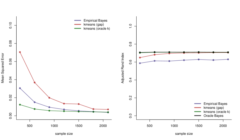
(a) Setting 1. Two equally sized clusters centered at $(0,0)$ and $(2,2)$. For clarification, in the ARI plot the red and green curves coincide.

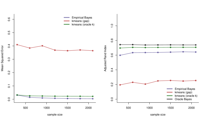
(b) Setting 2. Two clusters centered at $(0,0)$ and $(2,2)$ with cluster proportions $1/4$ and $3/4$.For clarification, in the ARI plot the red and green curves coincide.

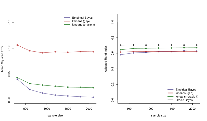
(c) Setting 3. Three clusters centered at $(0,0),(0,2),(2,-2)$ with cluster proportions $1/4,1/4,1/2$ respectively.

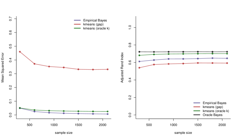
(d) Setting 4. Four cluster centers centered at $(0,0),(0,3),(3,0),(3,3)$ with cluster proportions drawn from Dirichlet distribution with parameters $(1,1,1,1)$

Figure 2: Empirical performance of methods in the denoising problem in four different clustering settings. A method with lower MSE is preferred over one with higher MSE. In contrast, a method with higher ARI is preferred over one with lower ARI. The lines show mean of the metric in question over $1000$ replicates.

From these MSE plots, it is clear that the Empirical Bayes estimates based on the NPMLE are more accurate than kmeans-gap. In fact, with the exception of the first setting, the Empirical Bayes estimates are even more accurate than kmeans-Oracle. This is probably because of the non-convexity of $k$-means.

In addition to estimating the means $\theta_{1},\dots,\theta_{n}$ by $\hat{\theta}_{1},\dots,\hat{\theta}_{n}$, the Empirical Bayes method also produces clusterings which can be compared to the true clusters (as well as to the clusterings produced by kmeans-Oracle and kmeans-gap) by the Adjusted Rand Index (ARI) [47]. Before showing these results, let us first explain how we are producing clusters based on the Empirical Bayes method. Our exemplar-based algorithm for computing the NPMLE based on $X_{1},\dots,X_{n}$ produces an estimate $\hat{f}_{n}$ which can be written as

$$\hat{f}_{n}(x):=\sum_{j=1}^{m}\hat{p}_{j}\phi_{d}(x-\hat{a}_{j})\qquad\text{for $x\in{\mathbb{R}}^{d}$}$$

for some $m\leq n$. From this estimate, we cluster the observation $X_{i}$ to the $r^{th}$ cluster (for $r=1,\dots,m$) provided

$$r=\mathop{\rm argmax}_{1\leq j\leq m}\frac{\hat{p}_{j}\phi_{d}(X_{i}-\hat{a}_{j})}{\sum_{l=1}^{m}\hat{p}_{l}\phi_{d}(X_{i}-\hat{a}_{l})}.$$

Note that the number of clusters $(=m)$ produced by this method will be different (and usually larger) than the true number of clusters but the ARI is applicable for comparing clusterings with different numbers of clusters. For comparison purposes, we also cluster using the true density where $\hat{p}_{j}$ and $\hat{a}_{j}$ in the method desribed above are replaced by $p_{j}$ and $a_{j}$ respectively with $f^{*}(x):=\sum_{j}p_{j}\phi_{d}(x-a_{j})$. We shall refer to this as the clustering based on the Oracle Bayes estimate.

For each of the these four clusterings (Empirical Bayes based clustering, kmeans-gap, kmeans-Oracle and Oracle Bayes based clustering), we plotted the ARIs as a function of sample size in Figure 2 (see the second plot in each pair of plots for the different settings). Higher ARIs are preferred to lower values. Here the Oracle Bayes estimate is the best; the kmeans-Oracle method is superior to the Empirical Bayes estimate as well as kmeans-gap. The comparison between the Empirical Bayes and the kmeans-gap estimates in terms of ARI can be summarized as follows. In the first setting, the performance of kmeans-gap is very good and is indistinguishable from kmeans-Oracle. In more complicated settings with more than two clusters and/or with imbalanced cluster proportions, a distinction between the two methods becomes apparent. In the second and fourth settings, the Empirical Bayes method outperforms kmeans-gap. In the third setting, the performances of the two methods start to coincide for larger sample sizes.

References

• Acharya et al. [2017] Acharya, J., I. Diakonikolas, J. Li, and L. Schmidt (2017). Sample-optimal density estimation in nearly-linear time. In Proceedings of the Twenty-Eighth Annual ACM-SIAM Symposium on Discrete Algorithms, pp.  1278–1289. SIAM.
• Balakrishnan et al. [2017] Balakrishnan, S., M. J. Wainwright, B. Yu, et al. (2017). Statistical guarantees for the em algorithm: From population to sample-based analysis. Ann. Statist. 45(1), 77–120.
• Barron et al. [1999] Barron, A., L. Birgé, and P. Massart (1999). Risk bounds for model selection via penalization. Probab. Theory Related Fields 113(3), 301–413.
• Bhaskara et al. [2015] Bhaskara, A., A. Suresh, and M. Zadimoghaddam (2015). Sparse solutions to nonnegative linear systems and applications. In Artificial Intelligence and Statistics, pp.  83–92.
• Birgé and Massart [1995] Birgé, L. and P. Massart (1995). From model selection to adaptive estimation. In D. Pollard, E. Torgersen, and G. L. Yang (Eds.), A Festschrift for Lucien Le Cam, pp.  55–87. New York: Springer-Verlag.
• Böhning [1995] Böhning, D. (1995). A review of reliable maximum likelihood algorithms for semiparametric mixture models. J. Statist. Plann. Inference 47(1-2), 5–28. Statistical modelling (Leuven, 1993).
• Böhning [1999] Böhning, D. (1999). Computer-assisted analysis of mixtures and applications, Volume 81 of Monographs on Statistics and Applied Probability. Chapman & Hall/CRC, Boca Raton, FL. Meta-analysis, disease mapping and others.
• Boucheron et al. [2013] Boucheron, S., G. Lugosi, and P. Massart (2013). Concentration inequalities. Oxford University Press, Oxford. A nonasymptotic theory of independence, With a foreword by Michel Ledoux.
• Brown [1971] Brown, L. D. (1971). Admissible estimators, recurrent diffusions, and insoluble boundary value problems. Ann. Math. Statist. 42, 855–903.
• Brown and Greenshtein [2009] Brown, L. D. and E. Greenshtein (2009). Nonparametric empirical Bayes and compound decision approaches to estimation of a high-dimensional vector of normal means. Ann. Statist. 37(4), 1685–1704.
• Chan et al. [2014] Chan, S.-O., I. Diakonikolas, R. A. Servedio, and X. Sun (2014). Efficient density estimation via piecewise polynomial approximation. In Proceedings of the forty-sixth annual ACM symposium on Theory of computing, pp.  604–613. ACM.
• Chan et al. [2013] Chan, S.-O., I. Diakonikolas, X. Sun, and R. A. Servedio (2013). Learning mixtures of structured distributions over discrete domains. In Proceedings of the twenty-fourth annual ACM-SIAM symposium on Discrete algorithms, pp.  1380–1394. SIAM.
• Chen et al. [2015] Chen, G. K., E. C. Chi, J. M. O. Ranola, and K. Lange (2015). Convex clustering: an attractive alternative to hierarchical clustering. PLoS computational biology 11(5), e1004228.
• Daskalakis and Kamath [2014] Daskalakis, C. and G. Kamath (2014). Faster and sample near-optimal algorithms for proper learning mixtures of gaussians. In Conference on Learning Theory, pp.  1183–1213.
• Dempster et al. [1977] Dempster, A. P., N. M. Laird, and D. B. Rubin (1977). Maximum likelihood estimation from incomplete data via the EM algorithm (with discussion). Journal of the Royal Statistical Society, Series B 39, 1–38.
• Devroye and Lugosi [2001] Devroye, L. and G. Lugosi (2001). Combinatorial methods in density estimation. Springer-Verlag.
• Dicker and Zhao [2016] Dicker, L. H. and S. D. Zhao (2016). High-dimensional classification via nonparametric empirical bayes and maximum likelihood inference. Biometrika 103(1), 21–34.
• Donoho and Reeves [2013] Donoho, D. and G. Reeves (2013). Achieving bayes mmse performance in the sparse signal+ gaussian white noise model when the noise level is unknown. In Information Theory Proceedings (ISIT), 2013 IEEE International Symposium on, pp.  101–105. IEEE.
• Efron [2011] Efron, B. (2011). Tweedie’s formula and selection bias. J. Amer. Statist. Assoc. 106(496), 1602–1614.
• Efron and Morris [1972] Efron, B. and C. Morris (1972). Empirical bayes on vector observations: An extension of stein’s method. Biometrika 59(2), 335–347.
• Efron and Morris [1976] Efron, B. and C. Morris (1976). Multivariate empirical bayes and estimation of covariance matrices. The Annals of Statistics, 22–32.
• Everitt and Hand [1981] Everitt, B. S. and D. J. Hand (1981). Finite mixture distributions. Chapman & Hall, London-New York. Monographs on Applied Probability and Statistics.
• Feng and Dicker [2016] Feng, L. and L. H. Dicker (2016). Nonparametric maximum likelihood inference for mixture models via convex optimization. arXiv preprint arXiv:1606.02011.
• Ghosal and van der Vaart [2007] Ghosal, S. and A. van der Vaart (2007). Posterior convergence rates of Dirichlet mixtures at smooth densities. Ann. Statist. 35(2), 697–723.
• Ghosal and van der Vaart [2001] Ghosal, S. and A. W. van der Vaart (2001). Entropies and rates of convergence for maximum likelihood and Bayes estimation for mixtures of normal densities. Ann. Statist. 29(5), 1233–1263.
• Hocking et al. [2011] Hocking, T. D., A. Joulin, F. Bach, and J.-P. Vert (2011). Clusterpath an algorithm for clustering using convex fusion penalties. In 28th international conference on machine learning, pp.  1.
• Jiang and Zhang [2009] Jiang, W. and C.-H. Zhang (2009). General maximum likelihood empirical Bayes estimation of normal means. Ann. Statist. 37(4), 1647–1684.
• Johnstone and Silverman [2004] Johnstone, I. M. and B. W. Silverman (2004). Needles and straw in haystacks: empirical Bayes estimates of possibly sparse sequences. Ann. Statist. 32(4), 1594–1649.
• Kiefer and Wolfowitz [1956] Kiefer, J. and J. Wolfowitz (1956). Consistency of the maximum likelihood estimator in the presence of infinitely many incidental parameters. Ann. Math. Statist. 27, 887–906.
• Koenker and Mizera [2014] Koenker, R. and I. Mizera (2014). Convex optimization, shape constraints, compound decisions, and empirical bayes rules. Journal of the American Statistical Association 109(506), 674–685.
• Laird [1978] Laird, N. (1978). Nonparametric maximum likelihood estimation of a mixed distribution. J. Amer. Statist. Assoc. 73(364), 805–811.
• Lashkari and Golland [2008] Lashkari, D. and P. Golland (2008). Convex clustering with exemplar-based models. In Advances in neural information processing systems, pp. 825–832.
• Li and Schmidt [2015] Li, J. and L. Schmidt (2015). A nearly optimal and agnostic algorithm for properly learning a mixture of k gaussians, for any constant k. arXiv preprint arXiv:1506.01367.
• Lindsay [1983a] Lindsay, B. G. (1983a). The geometry of mixture likelihoods: a general theory. Ann. Statist. 11(1), 86–94.
• Lindsay [1983b] Lindsay, B. G. (1983b). The geometry of mixture likelihoods. II. The exponential family. Ann. Statist. 11(3), 783–792.
• Lindsay [1995] Lindsay, B. G. (1995). Mixture models: theory, geometry and applications. In NSF-CBMS regional conference series in probability and statistics, pp.  i–163. JSTOR.
• Lindsay and Lesperance [1995] Lindsay, B. G. and M. L. Lesperance (1995). A review of semiparametric mixture models. J. Statist. Plann. Inference 47(1-2), 29–39. Statistical modelling (Leuven, 1993).
• Lindsten et al. [2011] Lindsten, F., H. Ohlsson, and L. Ljung (2011). Just relax and come clustering!: A convexification of k-means clustering. Linköping University Electronic Press.
• Massart [2007] Massart, P. (2007). Concentration inequalities and model selection. Lecture notes in Mathematics, Volume 1896. Berlin: Springer.
• Maugis and Michel [2011a] Maugis, C. and B. Michel (2011a). Data-driven penalty calibration: a case study for Gaussian mixture model selection. ESAIM Probab. Stat. 15, 320–339.
• Maugis and Michel [2011b] Maugis, C. and B. Michel (2011b). A non asymptotic penalized criterion for Gaussian mixture model selection. ESAIM Probab. Stat. 15, 41–68.
• Maugis-Rabusseau and Michel [2013] Maugis-Rabusseau, C. and B. Michel (2013). Adaptive density estimation for clustering with Gaussian mixtures. ESAIM Probab. Stat. 17, 698–724.
• McLachlan and Krishnan [2007] McLachlan, G. and T. Krishnan (2007). The EM algorithm and extensions, Volume 382. John Wiley & Sons.
• McLachlan and Peel [2004] McLachlan, G. and D. Peel (2004). Finite mixture models. John Wiley & Sons.
• Mosek [2015] Mosek, A. (2015). The mosek optimization toolbox for matlab manual. Version 7.1 (Revision 28), 17.
• Radchenko and Mukherjee [2014] Radchenko, P. and G. Mukherjee (2014). Consistent clustering using an $\ell_{1}$ fusion penalty. arXiv preprint arXiv:1412.0753.
• Rand [1971] Rand, W. M. (1971). Objective criteria for the evaluation of clustering methods. Journal of the American Statistical association 66(336), 846–850.
• Robbins [1950] Robbins, H. (1950). A generalization of the method of maximum likelihood-estimating a mixing distribution. In Annals of Mathematical Statistics, Volume 21, pp. 314–315.
• Robbins [1951] Robbins, H. (1951). Asymptotically subminimax solutions of compound statistical decision problems. In Proceedings of the second Berkeley symposium on mathematical statistics and probability, Volume 1, pp.  131–148.
• Robbins [1956] Robbins, H. (1956). An empirical bayes approach to statistics. In Proceedings of the Third Berkeley Symposium on Mathematical Statistics and Probability, Volume 1: Contributions to the Theory of Statistics, Berkeley, Calif., pp.  157–163. University of California Press.
• Robbins [1964] Robbins, H. (1964). The empirical bayes approach to statistical decision problems. The Annals of Mathematical Statistics 35(1), 1–20.
• Schlattmann [2009] Schlattmann, P. (2009). Medical applications of finite mixture models. Springer.
• Stein [1981] Stein, C. M. (1981). Estimation of the mean of a multivariate normal distribution. Ann. Statist. 9(6), 1135–1151.
• Suresh et al. [2014] Suresh, A. T., A. Orlitsky, J. Acharya, and A. Jafarpour (2014). Near-optimal-sample estimators for spherical gaussian mixtures. In Advances in Neural Information Processing Systems, pp. 1395–1403.
• Tan and Witten [2015] Tan, K. M. and D. Witten (2015). Statistical properties of convex clustering. Electronic journal of statistics 9(2), 2324.
• Tibshirani et al. [2001] Tibshirani, R., G. Walther, and T. Hastie (2001). Estimating the number of clusters in a data set via the gap statistic. Journal of the Royal Statistical Society: Series B (Statistical Methodology) 63(2), 411–423.
• Titterington et al. [1985] Titterington, D. M., A. F. M. Smith, and U. E. Makov (1985). Statistical analysis of finite mixture distributions. Wiley Series in Probability and Mathematical Statistics: Applied Probability and Statistics. John Wiley & Sons, Ltd., Chichester.
• Tsybakov [2009] Tsybakov, A. (2009). Introduction to Nonparametric Estimation. Springer-Verlag.
• Van der Vaart and Wellner [1996] Van der Vaart, A. and J. A. Wellner (1996). Weak Convergence and Empirical Process: With Applications to Statistics. Springer-Verlag.
• Wang et al. [2016] Wang, B., Y. Zhang, W. W. Sun, and Y. Fang (2016). Sparse convex clustering. arXiv preprint arXiv:1601.04586.
• Watanabe and Yamaguchi [2003] Watanabe, M. and K. Yamaguchi (2003). The EM algorithm and related statistical models. CRC Press.
• Weinstein et al. [2018] Weinstein, A., Z. Ma, L. D. Brown, and C.-H. Zhang (2018). Group-linear empirical bayes estimates for a heteroscedastic normal mean. Journal of the American Statistical Association, 1–13.
• Wong and Shen [1995] Wong, W. H. and X. Shen (1995). Probability inequalities for likelihood ratios and convergence rates of sieve mles. The Annals of Statistics, 339–362.
• Wu et al. [2016] Wu, C., S. Kwon, X. Shen, and W. Pan (2016). A new algorithm and theory for penalized regression-based clustering. Journal of Machine Learning Research 17(188), 1–25.
• Xie et al. [2012] Xie, X., S. Kou, and L. D. Brown (2012). Sure estimates for a heteroscedastic hierarchical model. Journal of the American Statistical Association 107(500), 1465–1479.
• Zhang [2009] Zhang, C.-H. (2009). Generalized maximum likelihood estimation of normal mixture densities. Statistica Sinica 19(3), 1297.
• Zhu et al. [2014] Zhu, C., H. Xu, C. Leng, and S. Yan (2014). Convex optimization procedure for clustering: Theoretical revisit. In Advances in Neural Information Processing Systems, pp. 1619–1627.