Generalized curvature modified plasma dispersion functions and Dupree renormalization of toroidal ITG

Abstract

A new generalization of curvature modified plasma dispersion functions is introduced in order to express Dupree renormalized dispersion relations used in quasi-linear theory. For instance the Dupree renormalized dispersion relation for gyrokinetic, toroidal ion temperature gradient driven (ITG) modes, where the Dupree’s diffusion coefficient is assumed to be a low order polynomial of the velocity, can be written entirely using generalized curvature modified plasma dispersion functions: $K_{nm}$’s. Using those, Dupree’s formulation of renormalized quasi-linear theory is revisited for the toroidal ITG mode. The Dupree diffusion coefficient has been obtained as a function of velocity using an iteration scheme, first by assuming that the diffusion coefficient is constant at each $v$ (i.e. applicable for slow dependence), and then substituting the resulting $v$ dependence in the form of complex polynomial coefficients into the $K_{nm}$’s for verification. The algorithm generally converges rapidly after only a few iterations. Since the quasi-linear calculation relies on an assumed form for the wave-number spectrum, especially around its peak, practical usefullness of the method is to be determined in actual applications.

I Introduction

I.1 Background

Most linear dispersion relations, relevant for kinetic waves in plasmas are described using combinations and/or generalizations of plasma dispersion functionsFried and Conte (1961). Many generalizations and modifications were proposed in the pastRobinson (1989); Summers and Thorne (1991); Hellberg and Mace (2002); Xie (2013) and efficiencies of the methods are comparedXie et al. (2017).

A particular such generalization is the introduction of the so called curvature modified plasma dispersion functions. These functions, which appear naturally in the formulation of the local, linear dispersion relation of the toroidal ion temperature gradient driven (ITG) mode, can be used to write the linear dispersion relations of various drift instabilities including ITG or its homologue the electron temperature gradient driven (ETG) mode in a generic form. Since the analytical continuation of these functions have already been incorporated in their definitions, they can be used in order to study damped modes as well as the usual unstable branches.

In this paper we introduce a further generalization of the curvature modified plasma dispersion functions which allows us to include a Dupree diffusion coefficient that has a velocity dependence in the form of a second order polynomial. This allows us to describe the perturbed or renormalized dispersion relations for toroidal drift instabilities using these functions.

The algorithm that we use in this paper is as follows. We start complex frequencies that are obtained as the solutions of the linear dispersion relation $\omega_{k}=\omega_{rk}+i\gamma_{k}$. Since the Dupree diffusion coefficient $D_{D}$ is usually defined in terms of itself via a complicated equation of the sort $D_{D}\sim\sum_{k}D_{0k}/\left(i\omega_{rk}+\gamma_{k}+D_{D}\right)$, we first compute it by taking it as zero on the right hand side. This gives us the first iteration $D_{D}^{\left(1\right)}$. Using $D_{D}=D_{D}^{\left(1\right)}$ in the perturbed dispersion equation$\varepsilon\left(\omega,\boldsymbol{k},D_{D}^{\left(1\right)}\left(v\right)\right)=0$, we compute the dominant renormalized complex frequency, which can be dubbed $\omega_{k}^{\left(1\right)}$. Using $D_{D}^{\left(1\right)}$ and $\omega_{k}^{\left(1\right)}$ we compute $D_{D}^{\left(2\right)}$ and so on, until the difference between $\left(D_{D}^{\left(n\right)}-D_{D}^{\left(n-1\right)}\right)/D_{D}^{\left(n-1\right)}$ is smaller than a predefined tolerance. The algorithm converges rapidly in only 3-4 iterations in most cases.

The paper is organized as follows.

I.2 Curvature modified dispersion functions

The functions, dubbed $I_{nm}\left(\zeta_{\alpha},\zeta_{\beta},b\right)$, and defined for $Im\left[\zeta_{\alpha}\right]>0$ as:

$$I_{nm}\left(\zeta_{\alpha},\zeta_{\beta},b\right)\equiv$$

$$\frac{2}{\sqrt{\pi}}\int_{0}^{\infty}dx_{\perp}\int_{-\infty}^{\infty}dx_{\parallel}\frac{x_{\perp}^{n}x_{\parallel}^{m}J_{0}^{2}\left(\sqrt{2b}x_{\perp}\right)e^{-x^{2}}}{\left(x_{\parallel}^{2}+\frac{x_{\perp}^{2}}{2}+\zeta_{\alpha}-\zeta_{\beta}x_{\parallel}\right)}\;\text{,}$$ (1)

can be written as a 1D integral of a combination of plasma dispersion functions as discussed in detail in Ref. Gürcan (2014):

$$I_{nm}\left(\zeta_{\alpha},\zeta_{\beta},b\right)=$$

$$\int_{0}^{\infty}s^{\frac{n-1}{2}}G_{m}\left(z_{1}\left(s\right),z_{2}\left(s\right)\right)J_{0}\left(\sqrt{2bs}\right)^{2}e^{-s}ds\;\mbox{,}$$

$$\quad(Im\left[\zeta_{\alpha}\right]>0)$$ (2)

using the straightforward multi-variable generalization of the standard plasma dispersion function: $G_{m}\left(z_{1},z_{2},\cdots,z_{n}\right)\equiv\frac{1}{\sqrt{\pi}}\int_{-\infty}^{\infty}\frac{x^{m}e^{-x^{2}}}{\prod_{i=1}^{n}\left(x-z_{i}\right)}dx$ with

$$z_{1,2}\left(s\right)=\frac{1}{2}\left(\zeta_{\beta}\pm\sqrt{\zeta_{\beta}^{2}-2\left(s+2\zeta_{\alpha}\right)}\right)\;\mbox{.}$$ (3)

The $G_{m}\left(z_{1},z_{2}\right)$ in (2) can be written in terms of the standard plasma dispersion function as:

$$G_{m}\left(z_{1},z_{2}\right) =\frac{1}{\sqrt{\pi}\left(z_{1}-z_{2}\right)}\bigg{[}z_{1}^{m}Z_{0}\left(z_{1}\right)-z_{2}^{m}Z_{0}\left(z_{2}\right)$$

$$+\sum_{k=2}^{m}\left(z_{1}^{k-1}-z_{2}^{k-1}\right)\Gamma\left(\frac{m-k+1}{2}\right)\bigg{]}\;,$$ (4)

which can be implemented using the Weideman method Weideman (1994).

Furthermore, in order to extend the validity of the definition (2) we must use $I_{nm}=I_{nm}^{{}^{\prime}}+\Delta I_{nm}$ [where $I_{nm}^{{}^{\prime}}$ is the integral in (2)], where

$$\Delta I_{nm}\left(\zeta_{\alpha},\zeta_{\beta},b\right)=-i\sqrt{\pi}2^{\frac{\left(n+3\right)}{2}}w^{\frac{n}{2}}\int_{-1}^{1}d\mu \left(1-\mu^{2}\right)^{\frac{\left(n-1\right)}{2}}\left(\mu\sqrt{w}+\frac{\zeta_{\beta}}{2}\right)^{m}$$

$$J_{0}^{2}\left(2\sqrt{b\left(1-\mu^{2}\right)w}\right)e^{-2\left(1-\mu^{2}\right)w-\left(\mu\sqrt{w}+\frac{\zeta_{\beta}}{2}\right)^{2}}\times\begin{cases}0&\zeta_{\alpha i}>0\quad\mbox{or }w_{r}<0\\ \frac{1}{2}&\zeta_{\alpha i}=0\quad\mbox{and }w_{r}>0\\ 1&\zeta_{\alpha i}<0\quad\mbox{and }w_{r}>0\end{cases}$$ (5)

with $w=\frac{\zeta_{\beta}^{2}}{4}-\zeta_{\alpha}$, $\zeta_{\alpha i}=\text{Im}\left(\zeta_{\alpha}\right)$ and $w_{r}=\text{Re}\left[w\right]$.

Derivatives of curvature modified dispersion functions can also be defined as analytical functions and implemented similarly Gültekin and Gürcan (2018).

I.3 Toroidal ITG

Following the kinetic formulation of toroidal ITG modeKim et al. (1994); Kuroda et al. (1998) starting from the linear gyrokinetic equationCatto (1978); Frieman and Chen (1982); Hahm (1988), which can be written in Fourier space for the non-adiabatic part of the distribution function as:

$$\bigg{(}\frac{\partial}{\partial t}+ iv_{\parallel}k_{\parallel}+i\hat{\omega}_{D}\left(v\right)\bigg{)}\delta g_{\boldsymbol{k}}$$

$$= \left(\frac{\partial}{\partial t}+i\omega_{*T}\left(v\right)\right)\frac{e}{T_{i}}\delta\Phi_{\boldsymbol{k}}F_{0}J_{0}\left(\frac{k_{\perp}v_{\perp}}{\Omega_{i}}\right)$$ (6)

Where $\hat{\omega}_{D}\left(v\right)=\frac{\omega_{D}}{2}\left(\frac{v_{\parallel}^{2}}{v_{ti}^{2}}+\frac{v_{\perp}^{2}}{2v_{ti}^{2}}\right)$, $\omega_{*Ti}\left(v\right)\equiv\omega_{*i}\left[1+\left(\frac{v^{2}}{2v_{ti}^{2}}-\frac{3}{2}\right)\eta_{i}\right]$, $\omega_{D}=2\frac{L_{n}}{R}\omega_{*i}$, $\omega_{*i}=v_{ti}\rho_{i}k_{y}/L_{n}$, $L_{n}=-\left(d\ln n_{0}/dr\right)^{-1}$, $\eta_{i}=d\ln T_{i}/d\ln n_{0}$, $R$ is the major radius of the tokamak, $v_{ti}$ is the ion thermal velocity, $\Omega_{i}$ is the ion cyclotron frequency and $\rho_{i}$ is the ion Larmor radius. The gyrokinetic equation is complemented by the quasi-neutrality relation, which is written here for adiabatic electrons for $k_{\parallel}\neq 0$:

$$\frac{e}{T_{e}}\delta\Phi_{k}=-\frac{e}{T_{i}}\delta\Phi_{k}+\int J_{0}\delta g_{k}d^{3}v\;\text{.}$$ (7)

Taking the Laplace-Fourier transform of (6), solving for $\delta g_{\mathbf{k},\omega}$ and substituting the result into (7), we obtain the following dispersion relation, written in terms of $\varepsilon\left(\omega,\mathbf{k}\right)$, the plasma dielectric function:

$$\varepsilon\left(\omega,\mathbf{k}\right)\equiv 1+\frac{1}{\tau}-P\left(\omega,\mathbf{k}\right)=0\;\text{.}$$ (8)

where

$$P\left(\omega,\mathbf{k}\right)=$$

$$\frac{1}{\sqrt{2\pi}v_{ti}^{3}}\int\frac{\left(\omega-\omega_{*Ti}\left(v\right)\right)J_{0}^{2}\left(\frac{k_{\perp}v_{\perp}}{\Omega_{i}}\right)e^{-\frac{v^{2}}{2v_{ti}^{2}}}}{\left(\omega-v_{\parallel}k_{\parallel}-\omega_{Di}\frac{1}{2}\left(\frac{v_{\parallel}^{2}}{v_{ti}^{2}}+\frac{v_{\perp}^{2}}{2v_{ti}^{2}}\right)\right)}v_{\perp}dv_{\perp}dv_{\parallel}$$

ormalising $k$ with $\rho_{i}^{-1}$ and Using $\omega/\left|k_{y}\right|\rightarrow\omega$, and $\omega_{D}/\left|k_{y}\right|\rightarrow\omega_{D}$, the dispersion relation (8) can be written as:

$$\varepsilon\left(\omega,\mathbf{k}\right)\equiv 1+\frac{1}{\tau}+\frac{1}{\omega_{Di}}\bigg{(}I_{10}\left[\omega+\left(1-\frac{3}{2}\eta_{i}\right)\right]$$

$$+\left(I_{30}+I_{12}\right)\eta_{i}\bigg{)}=0$$ (9)

where $I_{nm}\equiv I_{nm}\left(-\frac{\omega}{\omega_{Di}},-\frac{\sqrt{2}k_{\parallel}}{\omega_{Di}k_{y}},b\right)$ with $b\equiv k_{\perp}^{2}$.

II Generalized curvature modified dispersion functions

A further generalization of $I_{nm}$’s can be proposed in the form of the following integrals:

$$K_{nm}\left(\zeta_{a},\zeta_{b},\zeta_{c},\zeta_{d},b\right)=$$

$$\frac{2}{\sqrt{\pi}}\int_{0}^{\infty}dx_{\perp}\int dx_{\parallel}\frac{x_{\perp}^{n}x_{\parallel}^{m}J_{0}^{2}\left(\sqrt{2b}x_{\perp}\right)e^{-x^{2}}}{\left(x_{\parallel}^{2}+\zeta_{a}+\zeta_{b}x_{\parallel}+\zeta_{c}x_{\perp}+\zeta_{d}x_{\perp}^{2}\right)}$$ (10)

with complex variables $\zeta_{a}$, $\zeta_{b}$, $\zeta_{c}$ and $\zeta_{d}$, and the real variable $b$, so that, we can write

$$I_{nm}\left(\zeta_{\alpha},\zeta_{\beta},b\right)=K_{nm}\left(\zeta_{\alpha},-\zeta_{\beta},0,\frac{1}{2},b\right)\;\text{.}$$

The definition of the $I_{nm}$’s in terms of of the generalized plasma dispersion functions $G_{m}\left(z_{1},z_{2},\cdots,z_{n}\right)$ as in (2) can be extended to $K_{nm}$’s:

$$K_{nm}\left(\zeta_{a},\zeta_{b},\zeta_{c},\zeta_{d},b\right)=$$

$$2\int_{0}^{\infty}x_{\perp}^{n}G_{m}\left(z_{1}^{{}^{\prime}}\left(x_{\perp}\right),z_{2}^{{}^{\prime}}\left(x_{\perp}\right)\right)J_{0}\left(\sqrt{2b}x_{\perp}\right)^{2}e^{-x_{\perp}^{2}}dx_{\perp}\;\mbox{,}$$

using

$$z_{1,2}^{{}^{\prime}}\left(x_{\perp}\right)=\frac{1}{2}\left(-\zeta_{b}\mp\sqrt{\zeta_{b}^{2}-4\left(\zeta_{c}x_{\perp}+\zeta_{d}x_{\perp}^{2}+\zeta_{a}\right)}\right)\;\mbox{.}$$

Note that the function defined in (10) can represent any complex polynomial denominator up to second order in $x_{\parallel}$ and $x_{\perp}$. The resulting functions can be implemented using (4) to write the $G_{m}$’s and computing the remaining one dimensional $x_{\perp}$ integral using a numerical quadrature.

II.1 Analytical Continuation

The integral in (10) has a singularity in the complex plane when the polynomial in the denominator vanishes. Since the polynomial is a quadratic one that is a function of both $x_{\parallel}$ and $x_{\perp}$, it vanishes on a curve. If the coefficients were all real, this would be a curve in two dimensions. However since the coefficients are complex, the actual curve lives in 4 dimensional space made of $x_{\parallel r}$, $x_{\parallel i}$, $x_{\perp r}$ and $x_{\perp i}$ (i.e. real and imaginary parts of the extended $x_{\parallel}$ and $x_{\perp}$). However since it remains a “curve”, we can still parametrize it.

The analytical continuation of the $I_{nm}$’s are performed by first scaling the $x_{\perp}$ and $x_{\parallel}$ so that the ellipse becomes a circle, and then switching to polar coordinates so that the singularity becomes a point on the $r$ axis. The residue contribution is then equal to the integral over the angular variable on the circle. This residue is to be added to the original integral when $\text{Im}\left(\zeta_{\alpha}\right)<0$ and $w_{r}>0$ as shown in (5).

In the case of the $K_{nm}$ the issue is more complicated. Considering the denominator

$$d\left(x_{\perp},x_{\parallel}\right)=x_{\parallel}^{2}+\zeta_{b}x_{\parallel}+\zeta_{c}x_{\perp}+\zeta_{d}x_{\perp}^{2}+\zeta_{\alpha}$$

can be written using $\rho=\sqrt{\left(x_{\parallel}+\frac{\zeta_{br}}{2}\right)^{2}+\left(\sqrt{\zeta_{dr}}x_{\perp}\right)^{2}}$ and $\mu=\left(x_{\parallel}+\frac{\zeta_{br}}{2}\right)/\rho$ as:

$$d\left(\rho,\mu\right)= \rho^{2}\left(1+i\frac{\zeta_{di}\left(1-\mu^{2}\right)}{\zeta_{dr}}\right)$$

$$+\left(\zeta_{c}\frac{\sqrt{\left(1-\mu^{2}\right)}}{\sqrt{\zeta_{dr}}}+i\zeta_{bi}\mu\right)\rho-w$$

where $w=\frac{\zeta_{br}^{2}}{4}+i\frac{\zeta_{bi}\zeta_{br}}{2}-\zeta_{\alpha}$. The denominator becomes zero at the two complex roots:

$$\rho_{\pm}=-\frac{\beta}{2\alpha}\pm\frac{1}{2a}\sqrt{4\alpha w+\beta^{2}}$$ (11)

with $\alpha\equiv\left(1+i\frac{\zeta_{di}\left(1-\mu^{2}\right)}{\zeta_{dr}}\right)$ and $\beta\equiv\left(\zeta_{c}\frac{\sqrt{\left(1-\mu^{2}\right)}}{\sqrt{\zeta_{dr}}}+i\zeta_{bi}\mu\right)$.

Note that when we do the transformation from $x_{\perp}$, $x_{\parallel}$ to $\rho$ and $\mu$, the surface element becomes:

$$dx_{\perp}dx_{\parallel}=\frac{\rho}{\sqrt{\zeta_{dr}\left(1-\mu^{2}\right)}}d\mu d\rho$$

so that the integral can be written as:

$$K_{nm}\left(\zeta_{a},\zeta_{b},\zeta_{c},\zeta_{d},b\right)\equiv$$

$$\frac{2}{\sqrt{\pi}}\int_{-1}^{1}d\mu\int_{0}^{\infty}\rho d\rho\frac{x_{\perp}\left(\rho,\mu\right)^{n}x_{\parallel}\left(\rho,\mu\right)^{m}\left(J_{0}^{\rho}\right)^{2}e^{-x^{2}\left(\rho,\mu\right)}}{\alpha\left(\rho-\rho_{+}\right)\left(\rho-\rho_{-}\right)\sqrt{\zeta_{dr}\left(1-\mu^{2}\right)}}$$

where the shorthand notation $J_{0}^{\rho}=J_{0}\left(\sqrt{2b}x_{\perp}\left(\rho,\mu\right)\right)$ and $x^{2}\left(\rho,\mu\right)=x_{\perp}\left(\rho,\mu\right)^{2}+x_{\parallel}\left(\rho,\mu\right)^{2}$ has been used. This means that the residue contribution

$$\Delta K_{nm}\left(\zeta_{a},\zeta_{b},\zeta_{c},\zeta_{d},b\right)\equiv$$

$$4\sqrt{\pi}i\int_{-1}^{1}\rho_{+}d\mu\frac{x_{\perp}\left(\rho_{+},\mu\right)^{n}x_{\parallel}\left(\rho_{+},\mu\right)^{m}\left(J_{0}^{\rho_{+}}\right)^{2}e^{-x\left(\rho_{+},\mu\right)^{2}}}{\sqrt{4\alpha w+\beta^{2}}\sqrt{\zeta_{dr}\left(1-\mu^{2}\right)}}$$

should be added to the integral when $\text{Im}\left[\rho_{+}\left(\mu\right)\right]>0$ (and we should add $1/2$ times the residue contribution when $\text{Im}\left[\rho_{+}\left(\mu\right)\right]=0$). Note that writing the condition $\text{Im}\left[\rho_{+}\left(\mu\right)\right]>0$ in terms of real and imaginary parts of $\zeta$ parameters is complicated enough that we find it more practical to check this condition by computing $\rho_{+}$ using (11) numerically.

As a function of the real and imaginary parts of its primary variable $\zeta_{a}$, the function $K_{nm}$ can be plotted fixing the values of its other variables. The results are shown in figures 1 and 2.

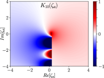
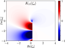
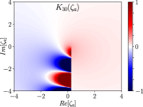
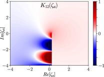
Figure 1: Plots of $K_{10}$, $K_{11}$, $K_{30}$ and $K_{12}$ (from top left to bottom right) as functions of the real and imaginary parts of $\zeta_{a}$, where the other parameters are fixed at $\zeta_{b}=1.0+0.5i$, $\zeta_{c}=0.5+0.5i$, $\zeta_{d}=0.5+0.2i$ and $b=1.0$.

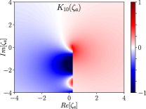
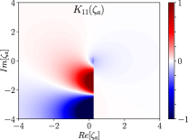
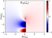
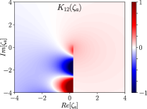
Figure 2: Plots of $K_{10}$, $K_{11}$, $K_{30}$ and $K_{12}$ (from top left to bottom right) as functions of the real and imaginary parts of $\zeta_{a}$, where the other parameters are fixed at the same parameters as figure 1 but with $\zeta_{c}=0.5+1.0i$.

III Dupree Renormalization

Dupree’s renormalized form of the gyrokinetic equation can be written asBalescu (2005); Krommes (2002):

$$\bigg{(}\frac{\partial}{\partial t}+ iv_{\parallel}k_{\parallel}+i\hat{\omega}_{D}\left(v\right)+D_{D}\left(v\right)k_{\perp}^{2}\bigg{)}\delta g_{\boldsymbol{k}}$$

$$= \left(\frac{\partial}{\partial t}+i\omega_{*T}\left(v\right)+D_{D}\left(v\right)k_{\perp}^{2}\right)\frac{e}{T_{i}}\delta\Phi_{\boldsymbol{k}}F_{0}J_{0}\left(\frac{k_{\perp}v_{\perp}}{\Omega_{i}}\right)\;\text{.}$$ (12)

Assuming a general complex $D_{D}\left(v\right)$, and short correlation times, we can write the discrete equivalent of Dupree’s integral equation as:

$$D_{D}\left(v_{\perp},v_{\parallel}\right)=\sum_{k}\frac{k^{2}J_{0k}^{2}\left|\delta\Phi_{k}\right|^{2}}{i\left(\omega_{k}^{*}-\omega_{Dk}\left(v\right)-k_{\parallel}v_{\parallel}\right)+D_{D}^{*}\left(v_{\perp},v_{\parallel}\right)k_{\perp}^{2}}$$ (13)

Note that here $\omega_{k}=\omega_{rk}+i\gamma_{k}$ is the solution of the renormalized linear dispersion relation due to (12):

$$\varepsilon\left(\omega,\mathbf{k}\right)\equiv 1+\frac{1}{\tau}$$

$$-\frac{1}{\sqrt{2\pi}v_{ti}^{3}}\int\frac{\left(\omega-\omega_{*Ti}\left(v\right)+iD_{D}\left(v\right)k_{\perp}^{2}\right)J_{0k}^{2}e^{-\frac{v^{2}}{2v_{ti}^{2}}}}{\omega-v_{\parallel}k_{\parallel}-\hat{\omega}_{Di}\left(v\right)+iD_{D}\left(v\right)k_{\perp}^{2}}v_{\perp}dv_{\perp}dv_{\parallel}$$ (14)

which is usually considered to introduce a nonlinear damping on top of the linear solution (i.e. $\omega_{k}=\omega_{k,\text{lin}}-i\eta_{\text{eddy}}$). This is exactly the case, if the Dupree diffusion coefficient is a real constant independent of $v$. However in the case of a complex function of $v_{\perp}$ and $v_{\parallel}$, the issue is more complicated.

One approach to this problem is to consider the dependence of $D_{D}$ on $v$ as being weak. This allows us to solve (13) at each $v$ seperately while considering $D_{D}$ as a constant in solving $\omega_{k}$ from (14). Of course this is only an intermediate step and one should finally consider a $v$ dependent $D_{D}\left(v\right)$ and somehow substitute that into (14) and show that $\omega_{k}$ that one can obtain together with the $D_{D}\left(v\right)$ gives us back the $D_{D}\left(v\right)$ that we used as a requirement of verification of this solution.

Unfortunately for an arbitrary function of $v$, this is hard to do. However when $D_{D}\left(v\right)$ is computed at each $v$ by assuming it as a constant in (14), the function that is obtained as a function of $v_{\parallel}$ or $v_{\perp}$ is rather close to a low order polynomial in a range of $v$ values. It means that we can fit a polynomial of the form

$$D_{D}=d_{0}+d_{1}x_{\parallel}+d_{2}x_{\parallel}^{2}+d_{3}x_{\perp}+d_{4}x_{\perp}^{2}$$ (15)

where $x_{\perp,\parallel}=v_{\perp,\parallel}/\sqrt{2}v_{ti}$, to the form obtained by solving (13) at each $v_{\perp}$ and $v_{\parallel}$. For simplicity we performed this fit by fixing $v_{\perp}=0$ and computing $D\left(v_{\parallel},0\right)$ and fitting and then fixing $v_{\parallel}=0$ and computing $D_{D}\left(0,v_{\perp}\right)$ and fitting.

For a given $v_{\perp}$, $v_{\parallel}$ we solve (13) by iteration. In practice we start the iteration by setting $D_{D}=0$ and computing $\omega_{k}$ from (12) and using this $\omega_{k}$ and $D_{D}=0$, we compute the perturbed $D_{D}$ using (13), which can be called $D_{D}^{\left(1\right)}$ since it is the first iteration. Then using this $D_{D}^{\left(1\right)}$ in (12), we can compute $\omega_{k}^{\left(1\right)}$ and substituting this $\omega_{k}^{\left(1\right)}$ and $D_{D}^{\left(1\right)}$ on the right hand side of (13), we obtain the $D_{D}^{\left(2\right)}$ and so on. We stop the iteration when convergence, defined by $\left|D_{D}^{\left(n\right)}-D_{D}^{\left(n-1\right)}\right|/\left|D_{D}^{\left(n-1\right)}\right|<\epsilon$ where the tolerance $\epsilon$ is taken to be around $\%1$. Fortunately it takes in general about $3$ iterations for this algorithm to converge.

One issue, which is a common problem in quasi-linear theory is that, a priori, one can not compute the spectrum $\left|\delta\Phi_{k}\right|^{2}$ that goes into (13) within the theory itself. Renormalization can be formulated in such a way that we could compute the spectrum using a local balance condition such as $D_{D}k_{\perp}^{2}\sim\gamma_{k}$. However while maybe the maximum of the spectrum could be determined from a condition of this form, the wave-number spectrum in plasma turbulence is well known to not follow the form implied by $D_{D}k_{\perp}^{2}\sim\gamma_{k}$ at every scale. In particular this is nonsensical when $\gamma_{k}$ becomes negative in some part of the $k$ space. Therefore here we chose to impose a reasonable form for the $k$-spectrum.

$$\left|\delta\Phi_{k}\right|^{2}=\begin{cases}e^{-\left(k-k_{0}\right)^{2}/2\sigma^{2}}&k<k_{p}\\ \left(e^{-\left(k_{p}-k_{0}\right)^{2}/2\sigma^{2}}k_{p}^{3}\right)k^{-3}&k>k_{p}\end{cases}$$

where $k_{0}$ is the maximum of the wave-number spectrum around which it is taken to be a gaussian with a width $\sigma$ which then joins a power law spectrum at the transition wave-number $k_{p}$. Obviously the $D_{D}$ that will be computed will depend on these parameters as well as the plasma parameters $R/L_{n}$, $\eta_{i}$ etc. Note that the exact form of this power law, or its refinment at higher $k$ for example by using a spectrum of the form $k^{-3}/\left(1+k^{2}\right)^{2}$ Gürcan et al. (2009) makes no practical difference for the computation of $D_{D}$. Finally we also take $k\rightarrow k_{y}$ above in order to keep the computation tracktable.

With all these assumptions, we can finally compute $D_{D}\left(v\right)$, the results are shown in figures 3 and 4. The coefficients of the polynomial (15) are computed in the two fits, with the parameters $\eta_{i}=2.5$, $L_{n}/R=0.2$, $k_{\parallel}=0.01$ and $k_{x}=0.1$ as:

$$d_{0} =0.08667974+0.04308331i$$

$$d_{3} =0.01342785+0.00293719i$$

$$d_{4} =-0.00176120+0.03260807i$$ (16)

and

$$d_{0} =0.08760955+0.04306338i$$

$$d_{1} =0.00034246+0.02108074i$$

$$d_{2} =0.02101908+0.02903672i\;\text{.}$$ (17)

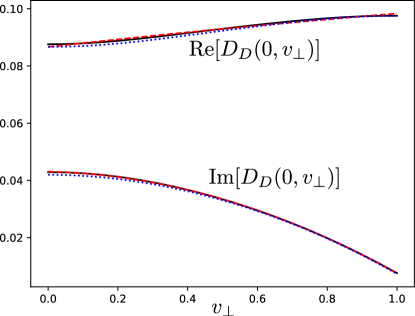
Figure 3: The real and imaginary parts of Dupree diffusion coefficient as a function of $v_{\perp}$. The solid (black) lines show the $D_{D}(0,v_{\perp})$ computed using iteration at each $v_{\perp}$ by assuming $D_{D}$ is constant in the dispersion relation, dashed (red) lines show the polynomial fit. The result that is obtained, when this polynomial fit is used to compute the $D_{D}$ again via (14) and (13), is shown as the (blue) dotted line.

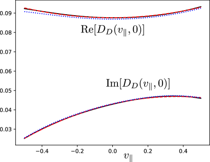
Figure 4: The real and imaginary parts of Dupree diffusion coefficient as a function of $v_{\parallel}$. The solid (black) lines show the $D_{D}(v_{\parallel},0)$ computed using iteration at each $v_{\parallel}$ by assuming $D_{D}$ is constant in the dispersion relation, dashed (red) lines show the polynomial fit. The result that is obtained, when this polynomial fit is used to compute the $D_{D}$ again via (14) and (13), is shown as the (blue) dotted line.

Since the two polynomials are consistent (i.e. $d_{0}$ is approximately the same in both cases), we can use these coefficients together in a single two dimensional polynomial form.

III.1 Solving the renormalized dispersion relation:

Until this point, we talked about solving the renormalized dispersion relation (14). While this is a simple matter of replacing $\omega\rightarrow\omega+ik_{\perp}^{2}D_{D}$ when $D_{D}$ is taken to be independent of $v$, when $D_{D}$ is taken to be of the form (15), the issue is more complicated. In this case, the dispersion relation have to be rewritten using the $K_{nm}$’s as follows:

$$\varepsilon\left(\omega,\mathbf{k}\right)\equiv 1+\frac{1}{\tau}+$$

$$\frac{1}{\omega_{Di}-id_{2}k_{\perp}^{2}}\bigg{[}\left(\omega-\omega_{*i}\left(1-\frac{3}{2}\eta_{i}\right)+ik_{\perp}^{2}d_{0}\right)K_{10}$$

$$+ik_{\perp}^{2}d_{3}K_{20}+\left(ik_{\perp}^{2}d_{4}-\omega_{*i}\eta_{i}\right)K_{30}$$

$$+\left(ik_{\perp}^{2}d_{2}-\omega_{*i}\eta_{i}\right)K_{12}+ik_{\perp}^{2}d_{1}K_{11}\bigg{]}=0$$ (18)

where $K_{nm}=K_{nm}\left(\zeta_{a},\zeta_{b},\zeta_{b},\zeta_{c},b\right)$ is used as a shortcut notation with

$$\zeta_{a}=-\frac{\omega+id_{0}k_{\perp}^{2}}{\omega_{Di}-id_{2}k_{\perp}^{2}}\;\text{,}\quad\zeta_{b}=\frac{\sqrt{2}k_{\parallel}v_{ti}-id_{1}k_{\perp}^{2}}{\omega_{Di}-id_{2}k_{\perp}^{2}}$$

$$\zeta_{c}=-\frac{id_{3}k_{\perp}^{2}}{\omega_{Di}-id_{2}k_{\perp}^{2}}\;\text{,}\quad\zeta_{d}=\frac{\frac{1}{2}\omega_{Di}-id_{4}k_{\perp}^{2}}{\omega_{Di}-id_{2}k_{\perp}^{2}}\;\text{.}$$

When the dispersion relation is written using the $K_{nm}$’s which are already analytic everywhere on the complex plane thanks to the analytical continuation discussed above, $\varepsilon\left(\omega,\mathbf{k}\right)$ also becomes analytic everywhere also. Note that the form used in (14) is actually not analytical when the imaginary part of $\rho_{+}$ as defined in (11) is greater than zero. Using a least square solver, we can then find the zeros of the renormalized dispersion relation and trace these results. The result with combined set of coefficients from (16) and (17) is shown in figure

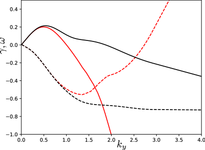
Figure 5: The growth rate (solid lines) and the frequency (dashed lines), with (red) and without (black) renormalization. Note that while the frequency changes sign and becomes positive, since the growth rate becomes strongly negative, it is unlikely that this positive frequency can actually be realized.

IV Results and Conclusions

Using a generalization of curvature modified plasma dispersion functions, we were able to implement a linear solver that can solve the dispersion relation with a Dupree diffusion coefficient in the form of a second order polynomial. The resulting solver was used in an algorithm based on iteration in order to solve the Dupree integral relation and therefore obtain the renormalized Dupree diffusion coefficient together with the renormalized growth rate and frequency for the gyrokinetic, local, electrostatic ITG, with adiabatic electrons.

Since the growth rate is obtained as the solution of the renormalized dispersion relation, it becomes rapidly negative for larg $k$ , in particular, due to the effect of Dupree diffusion. Thus, one has to define the generalized curvature modified plasma dispersion functions, the $K_{nm}$’s together with their analytical continuation. This guarantees that when the dispersion relation is written as in (18) using the $K_{nm}$’s it is also analytic everywhere in the complex plane.

The Dupree diffusion coefficient is rather important in quasi-linear transport formulationBourdelle et al. (2007), which has been developed into a full transport framework over the years Citrin et al. (2017), since in this formulation the effective correlation time is argued to be renormalized as compared to the linear one. It is also true that the heat flux in ITG should be proportional to the Dupree diffusion coefficientBalescu (2005).

The basic computation that is shown here is based on a number of assumptions such as a particular form that one has to assume for the $k$-spectrum, or the assumption that during the iteration procedure for every $v$ value one can at first assume that $D_{D}$ is a constant, etc. Nonetheless it proposes a numerically tractable, practical renormalization algorithm based on iteration including curvature effects. The algorithm can be generalized to include $k$ dependence of the eddy damping as well using a closure such as direct interaction approximation, or the eddy damped quasi-normal Markovian approximation, or rather its realizable variantLesieur (1997); Krommes (2002).

References

• Fried and Conte (1961) B. D. Fried and S. D. Conte, The Plasma Dispersion Function: The Hilbert Transform of the Gaussian. (Academic Press, London-New York, 1961) pp. v+419, erratum: Math. Comp. v. 26 (1972), no. 119, p. 814.
• Robinson (1989) P. A. Robinson, Journal of Mathematical Physics 30, 2484 (1989).
• Summers and Thorne (1991) D. Summers and R. M. Thorne, Physics of Fluids B: Plasma Physics 3, 1835 (1991).
• Hellberg and Mace (2002) M. A. Hellberg and R. L. Mace, Physics of Plasmas 9, 1495 (2002).
• Xie (2013) H. S. Xie, Physics of Plasmas 20, 092125 (2013).
• Xie et al. (2017) H. S. Xie, Y. Y. Li, Z. X. Lu, W. K. Ou,  and B. Li, Physics of Plasmas 24, 072106 (2017).
• Gürcan (2014) Ö. D. Gürcan, Journal of Computational Physics 269, 156 (2014).
• Weideman (1994) J. A. C. Weideman, SIAM J. Numer. anal. 31, 1497 (1994).
• Gültekin and Gürcan (2018) Ö. Gültekin and Ö. D. Gürcan, Plasma Physics and Controlled Fusion 60, 025021 (2018).
• Kim et al. (1994) J. Y. Kim, Y. Kishimoto, W. Horton,  and T. Tajima, Physics of Plasmas 1, 927 (1994).
• Kuroda et al. (1998) T. Kuroda, H. Sugama, R. Kanno, M. Okamoto,  and W. Horton, Journal of the Physical Society of Japan 67, 3787 (1998).
• Catto (1978) P. J. Catto, Plasma Physics 20, 719 (1978).
• Frieman and Chen (1982) E. A. Frieman and L. Chen, Physics of Fluids 25, 502 (1982).
• Hahm (1988) T. S. Hahm, Phys. Fluids 31, 2670 (1988).
• Balescu (2005) R. Balescu, Aspects of Anomalous Transport in Plasmas, Series in Plasma Physics (Institute of Physics, Bristol, UK, 2005).
• Krommes (2002) J. A. Krommes, Physics Reports 360, 1 (2002).
• Gürcan et al. (2009) Ö. D. Gürcan, X. Garbet, P. Hennequin, P. H. Diamond, A. Casati,  and G. L. Falchetto, Phys. Rev. Lett. 102, 255002 (2009).
• Bourdelle et al. (2007) C. Bourdelle, X. Garbet, F. Imbeaux, A. Casati, N. Dubuit, R. Guirlet,  and T. Parisot, Phys. Plasmas 14, 112501 (2007).
• Citrin et al. (2017) J. Citrin, C. Bourdelle, F. J. Casson, C. Angioni, N. Bonanomi, Y. Camenen, X. Garbet, L. Garzotti, T. Görler, O. Gürcan, F. Koechl, F. Imbeaux, O. Linder, K. van de Plassche, P. Strand,  and G. Szepesi , Plasma Physics and Controlled Fusion 59, 124005 (2017).
• Lesieur (1997) M. Lesieur, Turbulence in Fluids, third edition ed. (Kluwer, Dordrecht, 1997).