Google matrix of Bitcoin network

Abstract

We construct and study the Google matrix of Bitcoin transactions during the time period from the very beginning in 2009 till April 2013. The Bitcoin network has up to a few millions of bitcoin users and we present its main characteristics including the PageRank and CheiRank probability distributions, the spectrum of eigenvalues of Google matrix and related eigenvectors. We find that the spectrum has an unusual circle-type structure which we attribute to existing hidden communities of nodes linked between their members. We show that the Gini coefficient of the transactions for the whole period is close to unity showing that the main part of wealth of the network is captured by a small fraction of users.

1 Introduction

The bitcoin crypto currency was introduced by Satoshi Nakamoto in 2009 nakamoto and became at present an important source of direct financial exchange between private users wikibitcoin . At present this new cryptographic manner of financial exchange attracts a significant interest of society, computer scientists, economists and politicians (see e.g. bitcoinscience ; biryukov ; fedlet ; samuk ; cryptocurrency ). The amazing feature of bitcoin transactions is that all of them are open to public at blockchain that is drastically different from usual bank transactions deeply hidden from the public eye.

Since the data of bitcoin transaction network are open to public it is rather interesting to analyze the statistical properties of this Bitcoin network (BCN). Among the first studies of BTN we quote shamir and ober ; marcin where the statistical properties of BCN have been studied including the distribution of ingoing and outgoing transactions (links). Thus it was shown that a distribution of links is characterized by a power law ober ; marcin which is typical for complex scale-free networks dorogovtsev . Due to this it is clear that the methods of complex networks, such as the World Wide Web (WWW) and Wikipedia, should find useful applications for the BCN analysis. In particular, one can mention in this context the important PageRank algorithm brin which is at the foundation of the Google search engine meyer . Applications of this and related algorithms to various directed networks and related Google matrix are discussed in rmp2015 . Previous studies of the world trade network wtn1 ; wtn2 showed that for financial transactions or related trade of commodities it is useful to consider also the CheiRank probabilities for a network with inverted links linux and we will use this approach also here. In addition we analyze the spectrum of the Google matrix of BCN using the powerful numerical approach of the Arnoldi algorithm as described in ulamfrahm ; integer_network ; citation_network . We note that a possibility to use the PageRank probabilities for BCN was briefly noted in mit .

In our studies we use the bitcoin transaction data collected by Ivan Brugere from the public block chain site blockchain with all bitcoin transactions from the bitcoin birth in January 11th 2009 till April 2013 ivan .

The paper is composed as follows: In Section 2 we describe the main properties of BCN, the Google matrix is constructed in Section 3, the numerical methods of its analysis are described in Section 4, the spectrum and eigenvectors of $G$ matrix are analyzed in Sections 5 and 6, the Gini coefficient of BCN is determined in Section 7 and the discussion is given in Section 8.

2 Global BCN properties

From the bitcoin transaction data ivan of the period from the very beginning in January 11$th$ 2009 to April 10$th$ 2013, we construct the BCN and related Google matrix. This weighted and directed network takes into account the sum of all transactions, measured in units of bitcoin, from one user to another during a given period of time. The total number of transactions in this period is $N_{t}=28.140.756$. The minimum transaction value is $10^{-8}$ (was $10^{-3}$) bitcoin for the period after (before) march 2010.

The global statistical characteristics of transactions are shown in Figs. 1, 2, 3. Thus Fig.1 shows the frequency histogram $N_{f}(N_{a}),N_{f}(N_{b})$ of BCN in this period, given the dependencies for outgoing links (or sellers $N_{a}$), ingoing links (or buyers $N_{b}$), and transactions of the same partners from $a$ to $b$ ($N_{a,b}$). The fit of the data is in a satisfactory agreement with an algebraic decay $N_{f}\propto 1/{N_{a}}^{\beta}$, $N_{f}\propto 1/{N_{b}}^{\beta}$, $N_{f}\propto 1/{N_{a.b}}^{\beta}$ with $\beta=2.1\pm 0.1$, $\beta=1.8\pm 0.1$, $\beta=2.2\pm 0.1$ respectively.

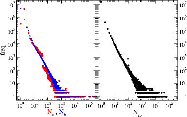
Figure 1: (color online) Frequency histograms of BCN $N_{f}$ in the period from January 11$th$ 2009 to April 10$th$ 2013. Left panel shows the frequency distribution $N_{f}$ of number of sellers (and buyers) transactions $N_{a}$ (and $N_{b}$). Right panel shows the frequency of transactions with the same given partners $N_{a,b}$.

Top panel of Fig.2 shows the histogram of bitcoin transaction volume $v_{m}$ for the whole period (2009-2013) measured in bitcoin. It is visible that it has peaks in values of $10^{-8},10^{-4}$ and $1$. At the same time there are also transactions with many bitcoins and $v_{m}$ as large as $834352.9$. The balance of each user $B_{u}$ can be defined as the sum of all ingoing transactions minus the outgoing ones measured in bitcoins. This balance $B_{u}$ is shown in the bottom panel of Fig.2. For a majority of users the balance is close to zero but in a few cases $B_{u}$ is strongly negative or positive. There are also visible peaks at values $B_{u}=30,25,20,10$.

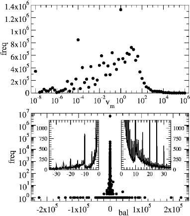
Figure 2: (color online) Frequency histogram $N_{f}$ of bitcoin transaction volume $v_{m}$ measured in bitcoins on top panel (histogram is equidistant in $\log_{10}v_{m}$ with a distance of $0.2$). Bottom panel shows the frequency histogram $N_{f}$ of user balance $B_{u}$ defined as the difference between ingoing and outgoing transactions in bitcoin units. Left and right insets show zoom in vicinity of zero balance for negative (left) and positive (right) values.

In order to study BCN time evolution we divide the whole period of time in year quarters from 2009 to 2013 (we take only half of years in 2009 since the number of transactions is very small). Some characteristic numbers of BCN are shown in Fig.3. There is a significant growth with time for the number of transactions $N_{t}$, and the integrated number of transactions $N_{it}$ (from the beginning till given quarter) and the number of nodes $N$ (partners) for the same period of time.

Figure 3: (color online) Characteristic evolution of BCN with year quarters (halves in 2009) from 2009 to April 2013. Time evolution is shown for number of transactions $N_{t}$ in a given quarter (black circles); number links $N_{it}$ of integrated transactions from the beginning till given quarter (red squares); number of nodes given by partners $N$ (green diamonds); and total volume of bitcoins (blue triangles).

At the next step we describe the construction of the Google matrix from the bitcoin transactions described above.

3 Construction of Google matrix of BCN

In this work we use the notation “BCYearQuarter” (e.g. BC2010Q2) for the different bitcoin networks, eventually with an additional “*” for the CheiRank case   (e.g. BC2010Q2*). We consider 16 (or 32 including the     CheiRank cases) networks BC2009Q2, BC2009Q4 to     BC2013Q2 with network sizes $N$ and link numbers $N_{\ell}$ ranging from $N=142$ and $N_{\ell}=117$ (BC2009Q2) to $N=6297009$ and $N_{\ell}=16056427$ (BC2013Q2) with typical ratios $N/N_{\ell}$ between $1$ for the smallest networks and $2.5-3$ for the largest networks. For the whole period of all quarters we have the total $G$ matrix size $N=6297539$ with $N_{\ell}=16056427$ links. The values of $N,N_{\ell}$ and total volume for all quarters are given in Table 1.

Network	$N$	$N_{\ell}$	total volume
			(in bitcoins)
BC2009Q2	142	117	51499
BC2009Q4	220	188	269526
BC2010Q1	645	632	681867
BC2010Q2	7706	11275	$2.33662\times 10^{6}$
BC2010Q3	37818	57437	$9.0931\times 10^{6}$
BC2010Q4	70987	111015	$1.86444\times 10^{7}$
BC2011Q1	204398	333268	$3.44654\times 10^{7}$
BC2011Q2	697401	1328505	$1.30747\times 10^{8}$
BC2011Q3	1547349	2857232	$2.0177\times 10^{8}$
BC2011Q4	1885400	3635927	$2.87714\times 10^{8}$
BC2012Q1	2186598	4395611	$3.2546\times 10^{8}$
BC2012Q2	2645532	5655802	$5.04581\times 10^{8}$
BC2012Q3	3742691	8381654	$1.02381\times 10^{9}$
BC2012Q4	4672122	11258315	$1.17078\times 10^{9}$
BC2013Q1	5998239	15205087	$1.29944\times 10^{9}$
BC2013Q2	6297009	16056427	$1.31479\times 10^{9}$

Table 1: Size ($N$), number of links ($N_{\ell}$) and total volume of used networks.

As usual we write the matrix associated to such a network as rmp2015 ; citation_network :

$$S=S_{0}+\frac{1}{N}\,e\,d^{T}$$ (1)

where $e^{T}=(1,\ldots,N)$ is the (transpose of the) uniform vector with unit entries, $d$ is the dangling vector with unit entries $d_{l}=1$ if $l$ corresponds to an empty column of $S_{0}$ and $d_{l}=0$ for the other columns. The elements $(S_{0})_{lk}$ of the matrix $S_{0}$ correspond to the value of the bitcoin transaction from a node $k$ to another node $l$ normalized by the total value of transactions from the node $k$ to all nodes. A similar construction of $S_{0}$ is used for the world trade network wtn1 . For the CheiRank case linux the direction of the transaction is inverted in this scheme, i.e. $(S_{0}^{*})_{lk}$ corresponds to the value of the bitcoin transaction from the node $l$ to $k$ normalized by the total value of transactions from all nodes to the node $k$. According to our raw data the bitcoin transactions up to 2010Q2 were done in units of $10^{-3}$ bitcoins and afterwards in units of $10^{-8}$ bitcoins. Therefore the raw transaction values and also the resulting (column sum normalized) entries of the matrix $S_{0}$ are rational numbers. For computations using normal precision numbers (i.e. standard double precision with a mantissa of 52 bits) these rational numbers can simply be replaced by the closest floating point number. However, for high precision computations using the library GMP gmplib , the precise rational values were kept as long as possible and, only when necessary, rounded to high precision floating point values with their maximal precision.

For the purpose of PageRank computations we also consider the Google matrix with damping factor $\alpha$ given by:

$$G=\alpha S+(1-\alpha)\frac{1}{N}\,e\,e^{T}$$ (2)

where we use $\alpha=0.85$ corresponding to its typical choice brin ; meyer ; rmp2015 . For the network with inverted direction of transactions, corresponding to the CheiRank case, we have $G^{*}=\alpha S^{*}+(1-\alpha)\frac{1}{N}\,e\,e^{T}$.

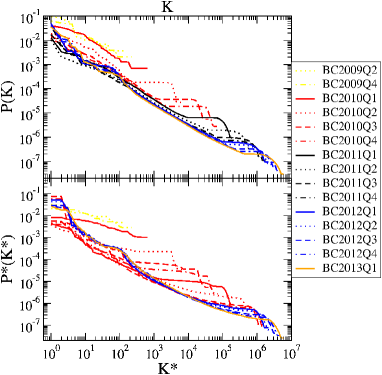
Figure 4: (color online) PageRank and CheiRank distributions ordered by indices $K$ and $K^{*}$ on top and bottom panel respectively. The bitcoin networks are taken by quarters of years (halves in the case of 2009) for 2009 (yellow), 2010 (red), 2011 (black), 2012 (blue) and 2013 (orange) with lines corresponding to Q1 (solid line), Q2 (dotted line), Q3 (dashed line) and Q4 (dot-dashed line).

The right eigenvectors $\psi_{m}$ of $G$ are determined by the equation $\sum_{j^{\prime}}G_{jj^{\prime}}\psi_{i}(j^{\prime})=\lambda_{i}\psi_{i}(j)$ with eigenvalues $\lambda_{i}$. At $\alpha<1$ the largest eigenvalue is $\lambda=1$ and the corresponding eigenvector has only positive component which have (for WWW networks) the meaning of probabilities $P(j)$ ($\sum_{j}P(j)=1$) to find a random surfer on a node $j$ meyer . We can order all nodes in the order of monotonic decrease of probability $P(K)$ with maximal probability at the PageRank index $K=1$ and then at $K=2,3...$. In a similar way for the CheiRank case of $G^{*}$ we obtain the CheiRank vector at $\lambda=1$ with CheiRank probability $P^{*}(K^{*})$ being maximal at the CheiRank index $K^{*}=1$ and then at $K^{*}=2,3...$. The PageRank vector is efficiently determined by the power iteration algorithm brin ; meyer .

The dependencies of the PageRank $P(K)$ and CheiRank $P^{*}(K^{*})$ probabilities on their indices $K,K^{*}$ are shown in Fig. 4 for various quarters of BCN. We see that the distributions become stabilized at last quarters when the network size becomes larger reaching its steady-state regime. Thus for BC2013Q1 we find that the probability approximately decays in a power law with $P\propto 1/K^{\nu},P^{*}\propto 1/{K^{*}}^{\nu}$ with $\nu=0.86\pm 0.06$, $\nu=0.73\pm 0.04$ respectively (the fit is done for the range $10<K,K^{*}<10^{5}$). The value of $\nu$ is similar to the values found for other directed networks (see e.g. rmp2015 ; wtn1 ; wtn2 ) but we note that this is only an approximate description of the numerically found behavior (see detailed discussion of algebraic decay for WWW networks in vigna ).

4 Numerical methods for BCN Google matrix diagonalization

We describe here the various skillful numerical methods used for diagonalization of $G$ and $G^{*}$. Their use had been required due to heavy numerical problems for accurate computation of the eigenvalues of these matrices and related eigenvectors.

First we introduce the concept of invariant isolated subsets (for more details we refer to fgsjphysa ). These subsets are invariant with respect to applications of $S$. The remaining nodes not belonging to an invariant subset (below a certain maximum size, e.g. 10% of the network size) form the wholly connected core space. The practical computation of these subsets can be efficiently implemented in a computer program fgsjphysa , eventually merging subspaces with common members, which provides a sequence of disjoint subspaces invariant by applications of $S$. Therefore we obtain a subdivision of the network nodes in $N_{c}$ core space nodes and $N_{s}$ subspace nodes (belonging to at least one of the invariant subsets) corresponding to the block triangular structure of the matrix $S$:

$$S=\left(\begin{array}[]{cc}S_{ss}&S_{sc}\\ 0&S_{cc}\\ \end{array}\right)\;\ .$$ (3)

Here $S_{ss}$ is composed of many small diagonal blocks for each invariant subspace and whose eigenvalues can be efficiently obtained by direct (“exact”) numerical diagonalization.

We have computed for the networks up to BC2011Q4 (with $N=1884918$ and $N_{\ell}=3635927$) (a part of) the complex eigenvalue spectrum of the matrix $S$ (i.e. $G(\alpha)$ for $\alpha=1$) with eigenvalues closest to the unit circle. For this we employed basically the method of Refs. fgsjphysa ; wikispectrum based on (3) to compute exactly the eigenvalues associated to the invariant subsets, typically a very modest number. For each invariant subspace there is at least one unit eigenvalue $\lambda=1$ which is therefore possibly degenerate (in case of several invariant subspaces). The remaining eigenvalues associated to the main core space (with $|\lambda|<1$) are obtained by the Arnoldi method arnoldibook ; ulamfrahm with Arnoldi dimensions up to $n_{A}=16000$. This requires for the network BC2011Q4 a machine with 256 GB (using standard double precision numbers).

For the larger networks (BC2012Q1 and later) it would be necessary to increase the available memory or to reduce the value of $n_{A}$. However, it turns out that the density of eigenvalues close to the unit circle is so high that a significant reduction of $n_{A}$ does not allow to obtain (even a small number) of reliable core space eigenvalues. This situation is quite different from other networks such as certain university networks fgsjphysa or Wikipedia wikispectrum where it was easier to access numerically a reasonable number of the top core space spectrum of the matrix $S$. Furthermore for the cases up to BC2011Q4 we also computed at least 20 eigenvectors of 20 selected (core space) eigenvalues close to the unit circle such that roughly $\lambda_{j}\approx|\lambda_{j}|\exp(i2\pi j/19)$ for $j=0,\ldots,19$ and $|\lambda_{j}|\approx 1$.

For the smallest bitcoin networks BC2009Q2,        BC2009Q4 and BC2010Q1 with $N\leq 645$ the core space eigenvalue spectrum is actually easily accessible by direct diagonalization or full Arnoldi diagonalization (with some subtle effects for the small eigenvalues requiring high precision computations).

The four networks BC2010Q2 and BC2010Q2*      (BC2010Q3 and BC2010Q3*) play a somewhat special role in our studies since on one hand they are sufficiently small with $N=7706$ (or $N=37818$) to allow (at least in theory) to compute all (or nearly all) non-zero eigenvalues and on the other hand they are still sufficiently large to have an interesting spectrum, comparable to the spectra of the larger networks, especially with a strong concentration of the majority of (non-vanishing) eigenvalues close to the unit circle.

However, it turns out that the two cases of BC2010Q2 and BC2010Q2* suffer from a serious numerical problem similar to the citation network of Physical Review citation_network . Using both direct diagonalization (i.e. using Householder transformations to transform the initial matrix to Hessenberg form and final diagonalization of the latter by the QR algorithm with implicit double shift) and full Arnoldi diagonalization (choosing a sufficiently large value of $n_{A}$ and QR algorithm to diagonalize the Arnoldi matrix which is also of Hessenberg form) with normal precision floating point numbers we find that there are several “rings” of eigenvalues close to the unit circle. The outer two rings seem to contain reliable and correct eigenvalues but already the third ring with $|\lambda|\approx 0.94$ and all rings below are numerically completely unreliable since the corresponding eigenvalues change completely between the two methods and also different implementations of them (i.e. applying a permutation in the network nodes but keeping the same network structure, choosing different ordering in the summation when computing the scalar products for the Arnoldi method, using slightly different but mathematical equivalent implementations of the QR algorithm, using different runs with parallelization which amounts to different rounding errors for the sums in the scalar products etc.). Therefore we conclude that eigenvalues with $|\lambda|<0.95$ are numerically incorrect as long as we use methods based on normal precision numbers.

This situation is quite similar to the (nearly) triangular citation network of Physical review citation_network where eigenvalues with $|\lambda|<0.4-0.5$ are numerically wrong. The reason of this behavior is due to large Jordan blocks for the highly degenerate zero eigenvalue producing numerically artificial rings of incorrect eigenvalues in the complex plane with radius $r\sim\varepsilon^{1/d}$ integer_network ; citation_network with $\varepsilon$ being the machine precision (i.e. $\varepsilon=10^{-16}$ for simple double precision numbers or $\varepsilon=2^{-p}$ for high precision numbers with $p$ binary digits) and $d\gg 1$ being the dimension of the Jordan block. The bitcoin networks do not have the (near) triangular structure, responsible for this problem in citation_network , but the low ratio of $N_{\ell}/N\approx 1.5$, reducing considerably the number of non-zero matrix elements in $S_{0}$, also creates large Jordan subspaces and here the effect is even worse as compared to Ref. citation_network .

To solve this problem and obtain final reliable eigenvalues with precision $10^{-15}$, we implemented all steps of the numerical diagonalization methods: the computation of the Arnoldi decomposition, reduction of an arbitrary matrix to Hessenberg form using Householder transformations, final diagonalization of Hessenberg matrices by the QR algorithm, with high precision floating point numbers using the GMP library gmplib . (In Ref. citation_network only the computation of the Arnoldi decomposition was implemented with the GMP library.).

For the two networks BC2010Q2 and BC2010Q2* we have been able to push the direct high precision diagonalization (Householder transformation to Hessenberg form and QR algorithm) with different precision up to $p=4096$ binary digits confirming the scaling $r\approx 2^{-p/d}$ for the radius of incorrect eigenvalues induced by large Jordan blocks. For $p=4096$ we find a maximal radius $r\approx 0.01$ corresponding to a value of $d\approx 616$ for the dimension of the corresponding Jordan block. In normal precision (with $p=52$) the same value of $d$ corresponds to a radius $\approx 0.94$ confirming exactly the observations of the initial normal precision results.

The direct diagonalization in high precision is however quite expensive in both computation time and memory requirement. In this context the (high precision) Arnoldi method is more efficient since it automatically breaks off when it has explored an $S$-invariant subspace which is detected by a vanishing or very small coupling matrix element in the Arnoldi matrix at some value of $n_{A}$ (see Refs. ulamfrahm ; citation_network for more details on this point). If we assume that the initial vector (which we chose either uniform or random with two different realizations) contains contributions from all eigenvectors associated to non-vanishing core space eigenvalues the method will, at least in theory, produce the complete spectrum of these eigenvalues using a considerably reduced subspace for the final (QR-) diagonalization. Here we have chosen a break off limit of $\epsilon=2^{-p/2}$ (with $p$ being the precision number of binary digits) for the final coupling matrix element which scales to zero with increasing precision but is still much larger than the computation precision ($2^{-p}$) allowing to take into account the subtle effects due to the Jordan blocks creating numerical errors on a scale much larger than the computation precision. In this case we obtain a reduced dimension of about 2000-3000 (depending on the choice of random or uniform initial vectors and on both cases of BC2010Q2 or BC2010Q2*) instead of 7706. Here the Arnoldi method with a precision of $p=8192$ binary digits (which is considerably less expensive than the direct diagonalization with $p=4096$) or even only $p=3072$ (for the case of BC2010Q2* with uniform initial vector) allows to obtain the complete spectra of non-vanishing eigenvalues for these two networks. The remaining small rings of numerical incorrect Jordan block induced eigenvalues can be easily removed from the correct eigenvalues by comparing the spectra obtained by different initial vectors.

We also employed (with some suitable technical modifications which we omit here) the rational interpolation method which we developed in Ref. citation_network . This method is also based on high precision computations to determine the zeros of a certain rational function which are the core space eigenvalues satisfying the condition $d^{T}\,\psi\neq 0$ for the corresponding eigenvector $\psi$ and the above introduced dangling vector $d$. It turns out that for the two networks BC2010Q2 and BC2010Q2* all non-vanishing core space eigenvalues satisfy this condition but for the other two networks BC2010Q3 and BC2010Q3* there a few core space eigenvalues with $d^{T}\,\psi=0$ which we determined separately by a method described in Ref. citation_network exploiting that they are degenerate subspace eigenvalues of the matrix $S_{0}$ (which are different from the subspace eigenvalues of $S$ which we also computed).

The rational interpolation method is highly effective with very modest memory requirements and the possibility to use partial low-precision spectra to accelerate the computation of the zeros to obtain recursively higher precision spectra. Here we obtained for BC2010Q2 and BC2010Q2* precise and complete spectra for $p=6144$ but we also performed confirmation runs up to $p=12288$. The results of this method confirm exactly the numerical values (with accuracy of $10^{-15}$ for all of the final eigenvalues) and the precise number of non-vanishing core space eigenvalues already obtained by the high precision Arnoldi method. We mention that the eigenvalues of the direct diagonalization correspond numerically with the same accuracy to these results (after removal of the numerically incorrect Jordan induced eigenvalues) but for $p=4096$ this method misses a small number (about $3-4$) of the smallest non-vanishing core space eigenvalues (with $|\lambda|\sim 5\times 10^{-3}$).

5 Spectrum of BCN Google matrix

We present here the main results obtained for the spectrum and some eigenvectors of $G$ and $G^{*}$ by the numerical methods described above.

For the two networks BC2010Q2 and BC2010Q2*, with a full network size of $N=7706$, we find that there are exactly $N_{c}=1967$ ($N_{c}=1984$) non-vanishing core space eigenvalues and $N_{s}=15$ ($N_{s}=2$) non-vanishing subspace eigenvalues (of $S$) for BC2010Q2 (or BC2010Q2*) with the complete and numerically accurate spectra shown in Fig. 5. The main two outer rings close to the unit circle (with $|\lambda|>0.97$) contain 1626 (1621) core space eigenvalues which is more than $80\%$ of the spectrum (of non-vanishing eigenvalues). The non-vanishing subspace eigenvalues $\lambda$, also shown in the same figure, and their multiplicities $m$ are $m=7$ ($\lambda=1$), $m=6$ ($\lambda=-1$), $m=1$ ($\lambda=-0.723606797749979$ and $\lambda=-0.276393202250021$) for BC2010Q2 and $m=1$ ($\lambda=\pm 1$) for BC2010Q2*. All other eigenvalues (about $\sim 5700$) are zero and correspond to Jordan subspaces with potentially rather large dimensions being responsible for the numerical problems when limiting the computations to normal floating point precision.

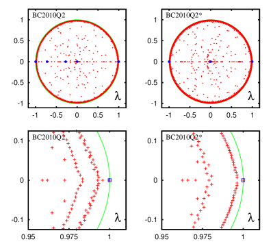
Figure 5: (Color online) Complex eigenvalue spectrum of the Google matrix associated to the network BC2010Q2 (BC2010Q2*) in left (right) panels. Shown are the full spectrum in top panels or a zoomed representation for the region $\lambda\approx 1$ in bottom panels. The red dots (crosses) are core space eigenvalues obtained by high precision Arnoldi computations and also the rational interpolation method and the blue thick dots (square boxes) are invariant subspace eigenvalues obtained by the normal/high precision Arnoldi method or direct diagonalization. The green line (if visible and not hidden by the red dots) is the unit circle. In top panels the apparent “red circle” corresponds in reality to a high density of individual red dots for the complex core space eigenvalues whose structure is better visible in the zoomed representation in bottom panels. The top core space eigenvalues (red crosses) which are very close to the top sub space eigenvalue at $\lambda=1$ (blue square box) are $0.99990029706715$ and $0.999678494064214$ (or $0.999998157039589$) for BC2010Q2 (BC2010Q2*). The 3rd top core space eigenvalue $0.995663863983884$ for BC2010Q2 is already clearly outside the blue square box. More details for the computation method and the subspace eigenvalues are given in the main text.

For the two networks BC2010Q3 and BC2010Q3*, with a full network size of $N=37818$, the numerical problems due to Jordan blocks for the zero eigenvalue are less severe but still present. Here the normal precision Arnoldi method allows to compute about 7800-7900 reliable eigenvalues within an error of $10^{-6}$ and which are rather strongly localized close to the boundary circle (if one tries larger values of $n_{A}$ one obtains only numerical incorrect eigenvalues). Here the high precision Arnoldi method is strongly limited due to memory requirements and it is not possible to go beyond a precision of $p=512$ which produces about 500-700 additional reliable eigenvalues and the resulting spectra are still quite concentrated close to the boundary circle. However, the rational interpolation method still works very well due to its high efficiency. It turns that at a binary precision of $p=30720$ using about 18400 support points (for the rational interpolation scheme) this method produces $N_{c}=9192$ ($N_{c}=9145$) non-vanishing core space eigenvalues (including 4 pairs of doubly degenerate eigenvalues in both cases). However, without going into technical details, our results indicate that these numbers may still increase very slightly when increasing the precision and also the number of support points but we are confident that for both networks BC2010Q3 and BC2010Q3* there are about $N_{c}\approx 9200$ non-vanishing core space eigenvalues which is about 25% of the full network size (a similar ratio we already found for BC2010Q2 and BC2010Q2*). The additional 1300-1400 eigenvalues with respect to the spectra obtained by the normal precision Arnoldi method fill out rather uniformly the inner part of the complex unit circle as can be seen in Fig. 6.

Furthermore for BC2010Q3 (BC2010Q3*) there also $N_{s}=56$ ($N_{s}=2$) subspace eigenvalues for $S$ (blue     dots/squares in Fig. 6). Here some eigenvalues are on the unit circle with $|\lambda|=1$ and degeneracy $m=23$ ($m=1$) for $\lambda=1$, $m=17$ ($m=1$) for $\lambda=-1$ and $m=2$ ($m=0$) for $\lambda=(-1\pm i\sqrt{3})/2$. In both cases there also a few core space eigenvalues (given as degenerate subspace eigenvalues of $S_{0}$, green dots) which were determined by another method citation_network since they are not necessarily found by the rational interpolation method. About $8000$ reliable eigenvalues are found by the normal precision Arnoldi method correspond to the 4-5 rings of eigenvalues close to the unit circle and visible in the center panels of Fig. 6.

Figure 6: (Color online) Complex eigenvalue spectrum of the Google matrix associated to the network BC2010Q3 (BC2010Q3*) in left (right) panels. Shown are the full spectra in top panels and two zoomed representations for the region $\lambda\approx 1$ in center and bottom panels. The red dots (crosses) are core space eigenvalues obtained by the rational interpolation method in high precision, the blue thick dots (square boxes) are invariant subspace eigenvalues obtained by the normal/high precision Arnoldi method or direct diagonalization and the thick green dots in top panels correspond to degenerate subspace eigenvalues of $S_{0}$ which are also core space eigenvalues of $S$ and not necessarily found by the rational interpolation method (see Ref. citation_network for explanations). There are 2 (is 1) top core space eigenvalue(s) (red cross(es)) very close to the top sub space eigenvalue at $\lambda=1$ i.e. nearly or completely inside the blue square box (in bottom panels) and the 1st top core space eigenvalue is $0.999968720409915$ ($0.99999983940032$) for BC2010Q3 (BC2010Q3*).

We mention that the high precision variants of the three methods are also useful to compute the full spectra for the three smaller networks (up to BC2010Q1 with $N=645$) and also for the invariant subspace spectra (for nearly all bitcoin networks) since they allow to remove in a reliable way a certain number of numerical incorrect eigenvalues below $10^{-3}$ obtained by the normal precision computations. For these cases the computation times are negligible and the required precision is rather modest (typically between $p=256$ and $p=1024$). Here the number of non-vanishing core space eigenvalues $N_{c}$ and subspace eigenvalues $N_{s}$ are given by $N_{c}=4$ ($6$) and $N_{s}=2$ ($0$) for BC2009Q2 (or BC2009Q2*) with $N=142$, $N_{c}=13$ ($15$) and $N_{s}=4$ ($2$) for BC2009Q4 (or BC2009Q4*) with $N=220$ and $N_{c}=26$ ($30$) and $N_{s}=6$ ($2$) for BC2010Q1 (or BC2010Q1*) with $N=645$. The subspace eigenvalues are always $\pm 1$ (except for BC2009Q2* where $N_{s}=0$ and there are no subspace eigenvalues) eventually with double (or triple) degeneracy if $N_{s}=4$ (or $N_{s}=6$). Clearly in all these cases the number of the non-vanishing core space and subspace eigenvalues constitutes only a small fraction of the spectrum with all other eigenvalues being zero corresponding to certain Jordan subspaces.

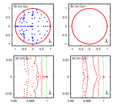
Figure 7: (Color online) Complex eigenvalue spectrum of the Google matrix associated to the network BC2011Q4 (BC2011Q4*) in left (right) panels. Shown are about 12000 “reliable” top eigenvalues obtained by the Arnoldi method in normal precision with $n_{A}=16000$ in top panels (red dots/red circle) or a zoomed representation (red crosses) for the region $\lambda\approx 1$ in bottom panels. The blue thick dots (square boxes) are invariant subspace eigenvalues obtained by the normal/high precision Arnoldi method or direct diagonalization. The green line (if visible and not hidden by the red dots) is the unit circle. In top panels the apparent “red circle” corresponds in reality to a high density of individual red dots for the complex core space eigenvalues whose structure is better visible in the zoomed representation. There are 8 (is 1) top core space eigenvalue(s) (red cross(es)) very close to the top sub space eigenvalue at $\lambda=1$ i.e. nearly or completely inside the blue square box and the 1st top core space eigenvalue is $0.99999999417$ ($0.99999996048$) for BC2011Q4 (BC2011Q4*).

For the larger networks (between BC2010Q4 with $N=70987$ and BC2011Q4 with $N=1884918$) we applied the normal precision Arnoldi method with $n_{A}=16000$. However, in view of the numerical problems visible for BC2010Q2/3, we performed different runs with slightly different implementations (e.g. different summation order for the scalar product in the Arnoldi method) leading to different rounding errors and verified how many eigenvalues were numerically identical with an error below $10^{-6}$. For the two cases BC2011Q4 and BC2011Q4* with $N=1884918$ and $n_{A}=16000$ we obtain about 12000 numerically reliable core space eigenvalues shown in Fig. 7 and which are all very close to the unit circle with $|\lambda|>0.99$. Fig. 7 also shows the subspace eigenvalues with $N_{s}=332$ ($2$) for BC2011Q4 (BC2011Q4*). The subspace spectrum of BC2011Q4 contains 242 eigenvalues on the unit circle with $|\lambda|=1$ which are $\lambda=1$ (degeneracy $m=127$), $\lambda=\pm i$ (both with $m=1$), $\lambda=(-1\pm i\sqrt{3})/2$ (both with $m=3$) and $\lambda=-1$ ($m=107$). The remaining 90 subspace eigenvalues with $0<|\lambda|<1$ are also visible in Fig. 7. Here only one eigenvalue at $\lambda=-1/2$ has a double degeneracy. The subspace spectrum of BC2011Q4* contains only the two (non-vanishing) eigenvalues $\lambda=\pm 1$ (both with $m=1$).

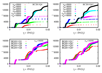
Figure 8: (Color online) Level number $j$ versus the decay width $\gamma_{j}=-2\ln(|\lambda_{j}|)$ with $\lambda_{j}$ being the $j$-th core space eigenvalue computed by the normal precision Arnoldi method with uniform initial vector and Arnoldi dimension $n_{A}$. The top left (right) panel corresponds to the network BC2011Q4 (or BC2011Q4*) for different values of $n_{A}$ with $2000\leq n_{A}\leq 16000$. The bottom left (right) panel corresponds to the four networks BC2011Qk, (or BC2011Qk*) for $k=1,2,3,4$ and $n_{A}=16000$.

The convergence with the increase of the Arnoldi dimension $n_{A}$ is illustrated in the top panels of Fig. 8 for BC2011Q4 showing the dependence $j(\gamma_{j})$ where     $\gamma_{j}=-2\ln|\lambda_{j}|$ with $\lambda_{j}$ being the core space eigenvalue. For $S$ and $S^{*}$ the comparison between the two maximal values $n_{A}=16000$ and $n_{A}=12000$ indicates that about $j\approx 5000-6000$ eigenvalues up to $\gamma\approx 0.01$ are reliable. However, we remind that the comparison of different computations for $n_{A}=16000$ shows that the number of reliable eigenvalues is actually higher $\approx 12000$ corresponding to $\gamma\approx 0.015$. The circle structure well visible in Fig. 7 is responsible for appearance of large steps in the dependence $j(\gamma)$ well seen in Fig. 8. A similar dependence $\gamma_{j}$ is also present for other quarters BC2011Q1, BC2011Q2, BC2011Q3 shown in bottom panels of Fig. 8.

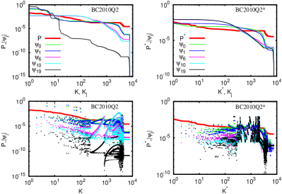
Figure 9: (Color online) Top panels: PageRank $P$ (or CheiRank $P^{*}$) at damping factor $\alpha=0.85$ and modulus $|\psi_{j}|$ of 5 selected eigenvectors of $S$ for the network BC2010Q2 (or BC2010Q2*) versus the index $K$ for PageRank $P$ ($K^{*}$ for CheiRank $P^{*}$) or the individual ordering index $K_{j}$ for each eigenvector $\psi_{j}$. Bottom panels: The same as top panels but only using the PageRank (CheiRank) index $K$ ($K^{*}$) on the $x$-axis for all shown vectors. Note that the given vector index values $0,1,6,10,19$ do not correspond to the level number of Fig. 8 but they correspond to an index of a selected set of 20 core space eigenvalues closest to the unit circle and with uniformly distributed eigenphases between 0 and $\pi$, i.e. the selected eigenvalues are roughly $\lambda_{j}\approx|\lambda_{j}|\exp(-i2\pi j/19)$ for $j=0,\dots,19$ and with $|\lambda_{j}|\approx 1$. In particular: $\lambda_{0}=0.99990030$ ($0.99999816$), $\lambda_{1}=0.99967849$ ($0.99612525+i0.00704040$), $\lambda_{6}=0.63708435+i0.75027164$ ($0.63887779+i0.75813987$), $\lambda_{10}=0.00130422+i0.98315766$ ($-0.00043259+i0.99066741$), and $\lambda_{19}=-0.99053491$ ($-0.99014386$) for BC2010Q2 (or BC2010Q2*).

6 Eigenstates of BCN Google matrix

The decay of PageRank and CheiRank probabilities at different quarters is presented in Fig. 4. Here we describe the properties of several eigenstates. As soon as the eigenvalues are determined the eigenstates corresponding to the selected eigenvalues can be efficiently computed numerically as described in rmp2015 ; ulamfrahm ; wikispectrum .

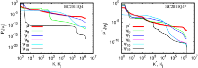
Figure 10: (Color online) PageRank $P$ (or CheiRank $P^{*}$) at damping factor $\alpha=0.85$ and modulus $|\psi_{j}|$ of 5 selected eigenvectors of $S$ for the network BC2011Q4 (or BC2011Q4*) versus the index $K$ for PageRank $P$ ($K^{*}$ for CheiRank $P^{*}$) or the individual ordering index $K_{j}$ for each eigenvector $\psi_{j}$. The given vector index is similar to Fig. 9. The eigenvalues of the shown eigenvectors are: $\lambda_{0}=0.99999999$ ($0.99999996$), $\lambda_{1}=0.99999322$ ($0.99907654$), $\lambda_{6}=0.64270357+i0.76431760$ ($0.64271106+i0.76429326$), $\lambda_{10}=-0.00116375+i0.99865094$ ($-0.00117162+i0.99862722$), and $\lambda_{19}=-0.99999317$ ($-0.99934321$) for BC2011Q4 (or BC2010Q4*).

The results for 6 eigenvectors of BC2010Q2 are shown in Fig. 9 and for BC2011Q4 in Fig. 10. The selected eigenvectors $\psi_{0}$, $\psi_{1}$, $\psi_{6}$, $\psi_{10}$, $\psi_{19}$ (additional to PageRank and CheiRank vectors) are marked by an index $j$ corresponding to 20 core eigenvalues closest to the unit circle with uniformly distributed eigenphases between $0$ and $\pi$. In the top panels of Fig. 9 we order all amplitudes $|\psi_{j}|$ in monotonically descending order with their own local-Rank index $K_{j}$ with maximum at $K_{j}=1$ ($K_{j}$ is different from PageRank index $K$). The interesting feature ofs these eigenstates is the presence of large plateaus where for hundreds of nodes the amplitude $|\psi_{j}|$ remains practically independent of $K_{j}$. This indicates a presence of relatively large communities of users coupled by certain links. The bottom panels of Fig. 9 show the amplitudes $|\psi_{j}|$ as a function of the global PageRank index $K$. For the BC2010Q2 network the nodes with largest amplitudes $|\psi_{j}|$ are located at relatively large $K$ values with $K<100$. It is possible that these nodes correspond to bitcoin miners. However, a significant number of nodes with relatively large amplitudes are located at very high values $K\sim 2000$. For the Google matrix $G^{*}$ all large amplitudes are located at large values of the CheiRank index $K^{*}>500$. For the larger BC2011Q4 network, shown in Fig. 10 we find the presence of similar plateau structure for eigenstate amplitudes.

Similarly to Wikipedia and other networks rmp2015 it is convenient to present the distribution of network nodes on the CheiRank-PageRank plane $(K,K^{*})$ shown in Fig. 11 for the cases of BC2010Q2 of Fig. 9 and BC2011Q4 of Fig. 10. We see that for BC2010Q2 the density distribution of $N$ nodes on $(K,K^{*})$-plane is still strongly fluctuating, but for BC2011Q4 it starts to stabilize and becomes close to the density of our largest network of BC2013Q2 shown in Fig. 12. The important feature of the stabilized density distributions of BC2011Q4 and BC2013Q2 is the fact that the maximum of distribution is located at the diagonal $K=K^{*}$. This is similar to the situation of the world trade network wtn1 ; wtn2 where each country (node) or user for BCN tries to keep trade balance between outgoing (export) and ingoing (import) flows.

In Fig. 11 we show by red crosses the location of top largest amplitudes $|\psi_{j}|$ at $j=10$ for Google matrices $G$ (left column) and $G^{*}$ (right column). We see that only a few large amplitudes are located at leading (smallest) values of $K$ and $K^{*}$. This shows that the vector $\psi_{10}$ corresponds to a certain rather isolated community.

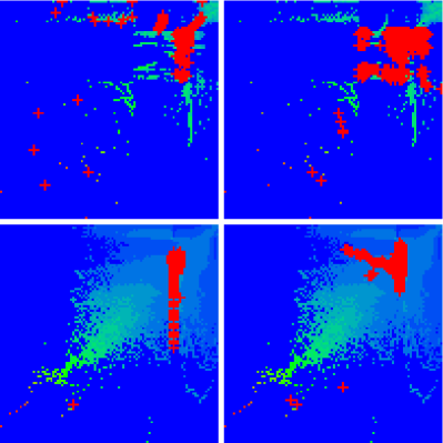
Figure 11: (Color online) Density of nodes $W(K,K^{*})$ on PageRank-CheiRank plane $(K,K^{*})$ averaged over $100\times 100$ logarithmically equidistant grids for $0\leq\ln K,\ln K^{*}\leq\ln N$, the density is averaged over all nodes inside each cell of the grid, the normalization condition is $\sum_{K,K^{*}}W(K,K^{*})=1$. Color varies from blue at zero value to red at maximal density value. In order to increase the visibility large density values have been reduced to (saturated at) 1/16 of the actual maximum density. At each panel the $x$-axis corresponds to $\ln K$ and the $y$-axis to $\ln K^{*}$. Both top panels correspond to BC2010Q2 for K and to BC2010Q2* for $K^{*}$ and both bottom panels to BC2011Q4 for K and to BC2011Q4* for $K^{*}$. The red crosses show the top 1000 nodes of the eigenvector $\psi_{10}$ used in Figs. 9 and 10 of BC2010Q2 (top left), BC2010Q2* (top right), BC2011Q4 (bottom left) and BC2011Q4* (bottom right).

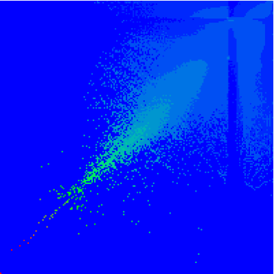
Figure 12: (Color online) Density of nodes $W(K,K^{*})$ on PageRank-CheiRank plane $(K,K^{*})$ for BC2013Q2 averaged over $200\times 200$ logarithmically equidistant grids for $0\leq\ln K,\ln K^{*}\leq\ln N$, the density is averaged over all nodes inside each cell of the grid, the normalization condition is $\sum_{K,K^{*}}W(K,K^{*})=1$. Color varies from blue at zero value to red at maximal density value. In order to increase the visibility large density values have been reduced to (saturated at) 1/16 of the actual maximum density. At each panel the $x$-axis corresponds to $\ln K$ and the $y$-axis to $\ln K^{*}$.

The proximity of the density distribution to the diagonal $K=K^{*}$ leads to a significant correlation between PageRank and CheiRank vectors $P(K(i))$ and $P^{*}(K^{*}(i))$. This correlation is convenient to characterized by the correlator rmp2015 ; linux ; wikispectrum $\kappa=N\sum_{i=1}^{N}P(K(i))P^{*}(K^{*}(i))-1$. The large values of $\kappa$ corresponds to a strong correlation of PageRank and CheiRank probabilities, while $\kappa$ close to zero or even slightly negative appears to uncorrelated vectors $P$ and $P^{*}$. The dependence of $\kappa$ on the network size $N$ is shown in Fig. 13 (right panel) where the correlator is becoming very large up to $\kappa\approx 10^{4}$ for the last quarters of BCN. The frequency distribution of correlator components $\kappa_{i}=NP(K(i))P^{*}(K^{*}(i))$ for three cases at different quarters is shown in the left panel of Fig. 13. These distribution show the presence of very active users with large $\kappa_{i}$ values corresponding to their expected high activity of bitcoin outgoing and ingoing transactions. It may be rather interesting to determine the hidden identity of users with largest $\kappa_{i}$ values.

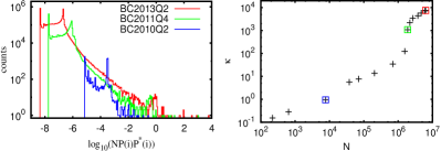
Figure 13: (Color online) Left panel: Histogram of frequency appearance of correlator components $\kappa_{i}=NP(K(i))P^{*}(K^{*}(i))$ for the three networks BC2013Q2 (red), BC2011Q4 (green) and BC2010Q2 (blue). For the histogram the whole interval $10^{-{9}}\leq\kappa_{i}\leq 10^{4}$ is divided in 260 cells of equal size in logarithmic scale. Right panel: The dependence of the correlator $\kappa=N\sum^{N}_{i=1}P(K(i))P^{*}(K^{*}(i))-1$ on the network size $N$ for all bitcoin networks between BC2009Q4 and BC2013Q2. The three data points surrounded by a colored square box correspond to the three networks of the left panel with the same colors.

7 Gini coefficient of BCN

In economy the distribution of wealth of a certain population is often characterized by the Gini coefficient proposed in 1912 (see e.g. gini1912 ; wikigini ; yakovenko ). The Gini coefficient is typically defined using the Lorenz curve which plots the fraction $y$ of the total income of a fraction $x$ of the population with the lowest income versus $x$. The line at $y=x$ thus represents perfect equality of incomes. The Gini coefficient is the ratio of the area that lies between the line of equality and the Lorenz curve normalized by the total area under the line of equality. Therefore the Gini coefficient is 0 for perfect equality and 1 for complete inequality.

We can generalize this definition to PageRank and CheiRank distributions. For this let $P(K)$ be the usual PageRank vector with $K=1$ for the maximum value corresponding to the top PageRank node. Then we define the inverted PageRank as $P_{\rm inv}(K^{\prime})=P(N-K^{\prime}-1)$ such that for $P_{\rm inv}$ the maximum value corresponds to $K^{\prime}=N$. In this way $P_{\rm inv}(K^{\prime})$ represents in a certain way the “income” and its argument $K^{\prime}$ corresponds to the network nodes ordered in increasing order by their income (with lowest “income” for $K^{\prime}=1$ and maximum “income” for $K^{\prime}=N$). Then the cumulative income up to node $K^{\prime}$ is given by :

$$\sigma(P)_{K^{\prime}} = \sum_{\tilde{K}=1}^{K^{\prime}}P_{\rm inv}(\tilde{K})=\sum_{\tilde{K}=N-K^{\prime}+1}^{N}P(\tilde{K}).$$ (4)

The notation $\sigma(P)$ reminds that $\sigma$ is defined with respect to a given PageRank vector (or CheiRank vector $P^{*}$ by replacing $P\to P^{*}$ in (4)). The quantity $\sigma(x)=\sigma(P)_{K^{\prime}}$ with $x=K^{\prime}/N$ corresponds to the standard Lorenz curve wikigini ; yakovenko . Therefore the Gini coefficient, defined as the area between $\sigma(P)$ and the line of equality normalized by the area below the line of equality wikigini , is given by:

$$g = 1-2\sum_{K^{\prime}=1}^{N}\sigma(P)_{K^{\prime}}/N=1-2\sum_{K=1}^{N}KP(K)/N.$$ (5)

The Gini coefficient for the CheiRank $P^{*}$ is obtained in a similar way by using $\sigma(P^{*})$ and replacing $P\to P^{*}$ in (5).

The above definition of $g$ is done via the PageRank and CheiRank probabilities, i.e. where “income” corresponds to the PageRank or CheiRank values. We will compare the corresponding $g$ values also with the standard definition considering ingoing and outgoing amount of bitcoins (volume transfer) for BCN nodes (users) during a given quarter. The dependence of the different Gini coefficients, defined via bitcoin volume transfer or PageRank and CheiRank probabilities, on time is shown in Fig. 14.

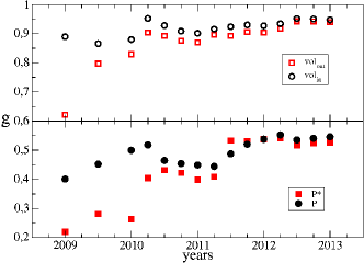
Figure 14: (Color online) Top panel: Gini coefficient $g$ time evolution for ingoing and outgoing bitcoin volume transfer for quarter of years (halves for 2009). Bottom panel: Gini coefficient $g$ time evolution for PageRank and CheiRank of BCN for quarter of years (halves for 2009).

Figure 15: (Color online) The Lorenz curve of the bitcoin users (nodes) showing $\sigma(P)_{K^{\prime}}$ (and $\sigma(P^{*})_{K^{*\prime}}$) vs. $K^{\prime}/N$ ($K^{*\prime}/N$) for PageRank and CheiRank of Q1 of 2010 and Q1 of 2013 (solid and dashed lines respectively). The Lorenz curves for cumulative volume transfer are also shown for the full period 2009-2013 for out-going and in-going flow, taking into account users with a minimum amount of 0 and 1 bitcoins (dotted and dot-dashed lines respectively). The Gini coefficient values for volume transfer are $g=0.948$ (in-going larger than 0), $g=0.939$ (out-going larger than 0), $g=0.927$ (in-going larger than 1), $g=0.925$ (out-going larger than 1). The blue solid line represents the curve of perfect equality.

For the BCN the evolution of Gini coefficient $g$, defined by (5), is shown in the bottom panel of Fig. 14. We find that the Gini coefficient defined via volume (top panel of Fig. 14) is stabilized from 2010 and takes a very high value $g\approx 0.9$. Such a large value of $g$ for bitcoin flows corresponds to an enormously unequal wealth distribution between users wikigini ; yakovenko : a small group of users controls almost all wealth.

We obtain smaller values of $g\approx 0.5$ for PageRank and CheiRank probabilities. We see that after 2010 the values of $g$ from PageRank and CheiRank probabilities become comparable. This corresponds to the stabilization of the node distribution in the PageRank - CheiRank plane (see Fig. 11, Fig. 12 discussed in the previous Section). After 2010 we find $g\approx 0.5$ corresponding to a rather usual value of $g$ with an exponential wealth distribution in a society (see e.g. yakovenko ). Also the Lorenz curve in 2013 (see Fig. 15) becomes similar to USA income distribution (see e.g. Fig.8 in yakovenko ).

However, the above values are obtained with the PageRank and CheiRank probabilities which are smoothing the row bitcoin flows due to the damping factor $\alpha$ in (2). For the row bitcoin flows for the whole available period 2009-2013 we find $g\approx 0.92$ (ingoing and outgoing $g$ values are rather close). Such high $g$ values correspond to very unbalanced wealth distribution in the bitcoin community.

8 Discussion

We presented the results of Google matrix analysis of bitcoin transaction network from the initial start in 2009 till April 2013. From the period after 2010 the PageRank and CheiRank probability distributions are stabilized showing an approximate algebraic decay with the exponent $\beta\approx 0.9$. We find that the spectrum of complex eigenvalues of matrix $G$ has a very unusual form of circles being rather close to the unitary circle. Such a structure has never appeared for other real networks reported previously rmp2015 . The only example with a similar spectral structure appears for the Ulam networks generated by intermittency maps maps . Such a circular structure corresponds to certain hidden communities coupled by a long series of transactions. A manifestation of such communities with about hundreds of users is also visible as a plateau structure in the eigenvectors of the Google matrix whose eigenvalues are close to the unit circle. The distribution of users in the PageRank-CheiRank plain is maximal along the diagonal corresponding to the the fact that each user tries to keep financial balance of his/her transactions. A similar situation was also observed for the world trade networks wtn1 ; wtn2 .

We also characterized the wealth distribution for BCN users using the Gini coefficient $g$. The definition of $g$ via PageRank and CheiRank probabilities leads to usual value $g\approx 0.5$ for the time period after 2010 when the BCN is well stabilized. However, the analysis of row bitcoin flows gives $g\approx 0.92$ corresponding to the situation when almost all wealth is concentrated in hands of small group of users. We argue that the damping factor of the Google matrix is responsible to a significant reduction of $g$ value.

Finally we note that the public access to all bitcoin transactions makes this system rather attractive for analysis of statistical features of financial flows. However, there is also a hidden problem of this network. In fact it often happens that a user performing a transaction to another user changes him/her bitcoin code after the transaction thus effectively creating a new user even if the person behind the code remains the same. This feature is responsible to the fact that the BCN is characterized by a rather low ratio of number of links to number of nodes being about 2-3 while in other networks like WWW and Wikipedia this ratio is about 10-20. This low ratio value is at the origin of the strong sensitivity of eigenvalues of $G$ to numerical computational errors as we discussed in the paper. Thus even if the bitcoin transactions are open to public it remains rather difficult to establish the transactions between real persons. In this sense the situation becomes similar to the transactions between bank units: in this case the data are not public and are hard to be accessed for scientific analysis.

We note that all data used in our statistical analysis of BCN are available at ourwebpage .

We thank A. D. Chepelianskii and S. Bayliss for stimulating discussions. This research is supported in part by the MASTODONS-2017 CNRS project APLIGOOGLE (see http://www.quantware.ups-tlse.fr/APLIGOOGLE/). This work was granted access to the HPC resources of CALMIP (Toulouse) under the allocation 2017-P0110.

References

- (1) Satochi Nakamoto, Bitcoin: A Peer-to-Peer Electronic Cash System, https://bitcoin.org/bitcoin.pdf (2008) (accessed 25 Oct 2017)
- (2) Wikipedia contributors, Bitcoin, https://en.wikipedia.org/wiki/Bitcoin_network, Wikipedia (accessed 25 Oct 2017)
- (3) J. Bohannon, The Bitcoin busts, Science 351, 1144 (2016)
- (4) A. Biryukov, D. Khovratovich and I. Pustogarov, Deanonymisation of clients in Bitcoin P2P network, Proc. 2014 ACM SIGSAC Conf. Comp. Comm. Security (CCS’14) ACM N.Y., p.15 (2014); arXiv:1405.7418v3[cs.CR] (2014)
- (5) F.R. Velde, Bitcoin: A primer, Chicago Fed Letter N.317, The Fderal Reserve Bank of Chicago, Dec. (2013).
- (6) S. Bayliss and L. Harriss, Financial Technology (FinTech), Houses of Parliament, Parliamentary Office of Science & Technology, Postnote Number 525, May (2016); http://researchbriefings.files.parliament.uk/documents/POST-PN-0525/POST-PN-0525.pdf (accessed 25 Oct 2017)
- (7) Wikipedia contributors, Cryptocurrency, https://en.wikipedia.org/wiki/Cryptocurrency, Wikipedia (accessed 25 Oct 2017)
- (8) https://blockchain.info/ (accessed 25 Oct 2017)
- (9) D. Ron and A. Shamir, Quantitative analysis of the full bitcoin transaction graph, in Sadeghi AR. (eds) Financial Cryptography and Data Security, FC 2013. Lecture Notes in Computer Science, 7859, 6 (2013), Springer, Berlin
- (10) M. Ober, S. Katzenbeisser and K. Hamacher, Structure and anonymity of the Bitcoin transaction graph, Future Internet 5, 237 (2013)
- (11) S.I. Marcin, Bitcoin Live: scalable system for detecting bitcoin network behaviors in real time, http://snap.stanford.edu/class/cs224w-2015/projects_2015/Bitcoin_Live-_Scalable_system_for_detecting_bitcoin_network_behaviors_in_real_time.pdf, Stanford (2015) (accessed 25 Oct 2017)
- (12) S. Dorogovtsev, Lectures on complex networks, Oxford University Press, Oxford (2010).
- (13) S. Brin and L. Page, Computer Networks and ISDN Systems 30, 107 (1998).
- (14) A.M. Langville and C.D. Meyer, Google’s PageRank and beyond: the science of search engine rankings, Princeton University Press, Princeton (2006).
- (15) L. Ermann, K.M. Frahm and D.L. Shepelyansky, Google matrix analysis of directed networks, Rev. Mod. Phys. 87, 1261 (2015).
- (16) L. Ermann and D. L. Shepelyansky, Google matrix of the world trade network, Acta Physica Polonica A 120(6A), A158 (2011).
- (17) L. Ermann and D. L. Shepelyansky, Google matrix analysis of the multiproduct world trade network, Eur. Phys. J. B 88, 84 (2015).
- (18) A.D. Chepelianskii, Towards physical laws for software architecture, arXiv:1003.5455 [cs.SE] (2010).
- (19) K. M. Frahm, and D. L. Shepelyansky, Ulam method for the Chirikov standard map, Eur. Phys. J. B 76, 57 (2010).
- (20) K. M. Frahm, A. D. Chepelianskii, and D. L. Shepelyansky, PageRank of integers, J. Phys. A: Math. Theor. 45, 405101(2012).
- (21) K. M. Frahm, Y.-H. Eom and D. L. Shepelyansky Google matrix of the citation network of Physical Review Phys. Rev. E 89, 052814 (2014).
- (22) M. Fleder, M.S. Kester and S. Pillai, Bitcoin transaction graph analysis, arXiv:1502.01657[cs/CR] (2015).
- (23) I. Brugere, Bitcoin transaction networks extraction, (2013) https://github.com/ivan-brugere/Bitcoin-Transaction-Network-Extraction (accessed Oct 2017).
- (24) T. Granlund and the GMP development team, GNU MP: The GNU Multiple Precision Arithmetic Library, http://gmplib.org/ (accessed Oct 2017).
- (25) K.M. Frahm, B. Georgeot and D.L. Shepelyansky, Universal emergence of PageRank, J. Phys. A: Math. Theor. 44, 465101 (2011).
- (26) L. Ermann, K.M. Frahm and D.L. Shepelyansky, Spectral properties of Google matrix of Wikipedia and other networks, Eur. Phys. J. B 86, 193 (2013).
- (27) G. W. Stewart, Matrix Algorithms, Volume II: Eigensystems, SIAM, (2001).
- (28) R. Meusel, S. Vigna, O. Lehmberg and C. Bizer, The graph structure in the web - analyzed on different aggregation levels, J. Web Sci. 1, 33 (2015)
- (29) C. Gini, Variabilita e mutabilita (1912), Reprinted in E. Pizetti, T. Salvemini (Eds.), Memorie di metodologica statistica, Libreria Eredi Virgilio Veschi, Rome (1955).
- (30) Wikipedia contributors, Gini coefficient, https://en.wikipedia.org/wiki/Gini_coefficient#CITEREFGini1912, Wikipedia (accessed 25 Oct 2017).
- (31) V. M. Yakovenko and J. B. Rosser Jr., Statistical mechanics of money, wealth, and income, Rev. Mod. Phys. 81, 1703 (2009).
- (32) L. Ermann and D.L. Shepelyansky, Google matrix of Ulam networks of intermittency maps, Phys. Rev. E 81, 036221 (2010).
- (33) http://www.quantware.ups-tlse.fr/QWLIB/bitcoinnet/ (accessed 3 Nov. 2017).