Exponential Lower Bounds on Spectrahedral Representations of Hyperbolicity Cones

Abstract

The Generalized Lax Conjecture asks whether every hyperbolicity cone is a section of a semidefinite cone of sufficiently high dimension. We prove that the space of hyperbolicity cones of hyperbolic polynomials of degree $d$ in $n$ variables contains $(n/d)^{\Omega(d)}$ pairwise distant cones in the Hausdorff metric, and therefore that any semidefinite representation of such polynomials must have dimension at least $(n/d)^{\Omega(d)}$ (even allowing a small approximation error). The cones are perturbations of the hyperbolicity cones of elementary symmetric polynomials. Our proof contains several ingredients of independent interest, including the identification of a large subspace in which the elementary symmetric polynomials lie in the relative interior of the set of hyperbolic polynomials, and a quantitative generalization of the fact that a real-rooted polynomial with two consecutive zero coefficients must have a high multiplicity root at zero.

1 Introduction

A homogeneous polynomial $p$ in $\mathbb{R}[x_{1},\ldots,x_{n}]$ is said to be hyperbolic with respect to a direction $e\in\mathbb{R}^{n}$ if $p(e)\neq 0$ and all its univariate restrictions along the direction $e$ are real-rooted, i.e., for every $x\in\mathbb{R}^{n}$, the polynomial $p_{x}(t)=p(te+x)$ has all real roots. Gårding showed that every hyperbolic polynomial $p$ is associated with a closed convex cone $K_{p}$ defined as follows,

$$K_{p}=\{x\in\mathbb{R}^{n}|\text{ all roots of }p(te+x)\text{ are non-positive}\}.$$

The cone $K_{p}$ is referred to as the hyperbolicity cone associated with the polynomial $p$.

From the standpoint of convex optimization, hyperbolicity cones yield a rich family of convex sets that one can efficiently optimize over — in particular, interior point methods can be used to efficiently optimize over the hyperbolicity cone $K_{p}$ for a polynomial $p$, given an oracle to evaluate $p$ and its gradient and Hessian [Gül97, Ren06]. This optimization primitive, referred to as hyperbolic programming, captures linear and semidefinite programming as special cases. Specifically, the hyperbolicity cone for the polynomial $p(x_{1},\ldots,x_{n})=\prod_{i=1}^{n}x_{i}$ is the positive orthant $\mathbb{R}_{+}^{n}$, which corresponds to linear programming, while semidefinite programming arises from the symmetric determinant polynomial $\det(X)$. Is hyperbolic programming as an algorithmic primitive strictly more powerful than semidefinite programming? Can hyperbolicity cones other than these two be harnessed towards obtaining better algorithms for combinatorial optimization problems? These compelling questions remain open.

Lately, the relationship between hyperbolicity cones and the semidefinite cone has been a subject of intense study. It is easy to see that every section of the semidefinite cone is a hyperbolicity cone, so it is natural to ask whether the converse holds, i.e., if every hyperbolicity cone can be realized as a section of the semidefinite cone. Formally, a spectrahedral cone $K$ is specified by:

$$K=\{x\in\mathbb{R}^{n}\mid\sum_{i}A_{i}x_{i}\succeq 0\},$$

for some matrices $\{A_{i}\}_{i\in[n]}\in\mathbb{R}^{B\times B}$. It is conjectured that every hyperbolicity cone is a spectahedral cone.

Conjecture 1.

(Generalized Lax Conjecture) Every hyperbolicity cone is a spectahedral cone, i.e., a linear section of the cone of positive semidefinite matrices in some dimension.

The Lax conjecture in its original stronger algebraic form asked whether every polynomial in three variables hyperbolic with respect to the direction $(1,0,0)$, could be written as $\det(xI+yB+zC)$ for some symmetric matrices $B,C$ (sometimes called a definite determinantal representation). This immediately implies that all hyperbolicity cones in three dimensions are spectrahedral, and was proved by Helton and Vinnikov and Lewis, Parrilo, and Ramana [HV07, LPR05]. The algebraic conjecture is easily seen to be false for $n>3$ by a count of parameters, since the set of hyperbolic polynomials is known to have nonempty interior [Nui69] and is of dimension $n^{d}$, whereas the set of $n-$tuples of $d\times d$ matrices has dimension $n\binom{d}{2}$. This led to the weaker conjecture that for every hyperbolic $p(x)$ there is an integer $k$ such that $p(x)^{k}$ admits a definite determinantal representation, which was disproved by Bränden in [Brä11]. The Generalized Lax conjecture, which is a geometric statement, is equivalent to the yet weaker algebraic statement that for every hyperbolic $p(x)$ there is a hyperbolic $q(x)$ such that $K_{p}\subseteq K_{q}$ and $p(x)q(x)$ admits a definite determinantal representation.

For several special classes of hyperbolic polynomials, the corresponding hyperbolicity cones are known to be spectrahedral. The elementary symmetric polynomial of degree $d$ in $n$ variables is given by $e_{d}(x)=\sum_{S\subseteq[n],|S|=d}\prod_{i\in S}x_{i}$. Bränden [Brä14] showed that the hyperbolicity cones of elementary symmetric polynomials are spectrahedral with matrices of dimension $O(n^{d})$. If a polynomial $p$ is hyperbolic with respect to a direction $e\in\mathbb{R}^{n}$, then its directional derivatives along $e$ are hyperbolic too [Går59]. Directional derivatives of the polynomial $p(x)=\prod_{i\in[n]}x_{i}$ [Zin08, San13, Brä14, COSW04] and the first derivatives of the determinant polynomial [Sau17] are also known to satisfy the generalized Lax conjecture. Amini [Ami16] has shown that certain multivariate matching polynomials are hyperbolic and that their cones are spectrahedral, of dimension $n!$.

Given the above examples, it is natural to wonder whether exponential blowup in dimension is an essential feature of passing from hyperbolicity cones to spectrahedral representations, and even assuming the generalized Lax conjecture to be true, the size of the spectrahedral representation of a hyperbolicity cone is interesting from a complexity standpoint. In this paper, we obtain exponential lower bounds on the size of the spectrahedral representation in general, even if the representation is allowed to be approximate (up to an exponentially small error).

Recall that the Hausdroff distance between two cones $K$ and $K^{\prime}$ is defined as

$$\mathsf{hdist}(K,K^{\prime})=\max_{x\in\mathcal{B}\cap K,y\in\mathcal{B}\cap K^{\prime}}(d(x,K^{\prime}),d(y,K)),$$

where $\mathcal{B}$ is the unit ball in $\mathbb{R}^{n}$. We say that a spectrahedral cone $K^{\prime}$ is an $\eta$-approximate spectrahedral representation of another cone $K$ if $\mathsf{hdist}(K,K^{\prime})\leq\eta$. Our main theorem is the following.

Theorem 2 (Main Theorem).

There exists an absolute constant $\kappa>0$ such that for all sufficiently large $n,d$, there exists an n-variate degree $d$ hyperbolic polynomial $p$ whose hyperbolicity cone $K_{p}$ does not admit an $\eta-$approximate spectrahedral representation of dimension $B\leq\left(n/d\right)^{\kappa d}$, for $\eta=1/n^{4nd}$.

Our proof is analytic and does not rely on algebraic obstacles to representability; in fact the polynomials we construct have very simple coefficients (they are essentially binary perturbations of $e_{d}$). However, since there are $\binom{n}{d}$ coefficients, the examples require $\Omega(n^{d})$ bits to write down. It is still unknown whether $e_{d}$ itself admits a low dimensional spectrahedral representation, though Saunderson and Parrilo [SP15] have shown that if one allows projections of sections of semidefinite cones, then such a represntation exists with size $\mathrm{poly}(n,d)$.

Algebraically, the notion of (exact) spectrahedral representation of a hyperbolicity cone $K_{p}$ for a polynomial $p$ corresponds to an algebraic identity of the form,

$$p(x)\cdot q(x)=det(\sum_{i\in[n]}C_{i}x_{i})\ ,$$

where $K_{q}$ contains $K_{p}$. Thus, our main theorem implies the existence of a degree $d$ polynomial $p$ such that the degree of any identity of the above form is at least $(n/d)^{\kappa d}$.

1.1 Proof Overview

The starting point for our proof is the theorem of Nuij [Nui69], which says that the space of hyperbolic polynomials of degree $d$ in $n$ variables has a nonempty interior, immediately implying that it has dimension $n^{d}$. The Generalized Lax Conjecture concerns the cones of these polynomials, which are geometric rather than algebraic objects. If we could show that this space of cones also has large “dimension” in some appropriate quantitative sense, and that the maps between the hyperbolicity cones and their spectrahedral representations are suitably well-behaved, then it would rule out the existence of small spectrahedral representations for all of them uniformly, since such representations are parameterized by tuples of $n$ $B\times B$ matrices, which have dimension $nB^{2}$.

The difficulties in turning this idea into a proof are: (1) There are no quantitative bounds on Nuij’s theorem. (2) the space of hyperbolicity cones is hard to parameterize and it is not clear how to define dimension. (3) the mapping from hyperbolicity cones to their representations can be arbitrary, and needn’t preserve the usual notions of dimension anyway. We surmount these difficulties by a packing argument, which consists of the following steps.

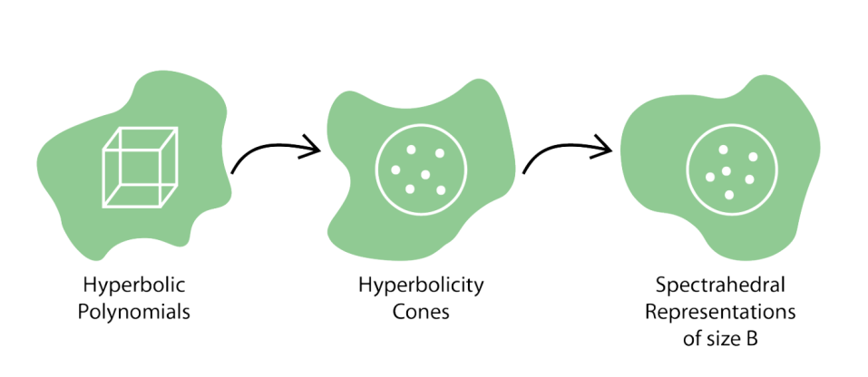
Figure 1: Outline of the Proof

1. Exhibit a large family of hyperbolicity cones of size $2^{(n/d)^{\Omega(d)}}$, every pair of which are at least $\epsilon$ apart from each other in the Hausdroff metric between the cones.

2. Show that the spectrahedral representations of two distant cones $K$ and $K^{\prime}$ are distant from each other, once the representations are appropriately normalized. Formally, the matrices $\{C_{i}\}_{i\in[n]}$ and $\{C^{\prime}_{i}\}_{i\in[n]}$ representing the two cones are at least $\epsilon^{\prime}$ away in operator norm if $\mathsf{hdist}(K,K^{\prime})\geq\epsilon$ (see Lemma 14).

   We work only with cones which contain the positive orthant in order to ensure that they have normalized representations.

3. By considering the volume, there is a $(B/\epsilon^{\prime})^{nB^{2}}$ upper bound on the number of pairwise $\epsilon^{\prime}$-distant spectrahedral representations in $B\times B$ matrices, thus giving the lower bound on $B$.

By far, the most technical part of the proof is the first step exhibiting a large family of pairwise distant hyperbolicity cones. The set of hyperbolic polynomials is known to have a non-empty interior in the set of all degree $d$ homogenous polynomials. Although this implies the existence of a full-dimensional family of hyperbolic polynomials, it is not clear how far apart they are quantitatively. Moreover, without any further understanding of the structure of the polynomials, it is difficult to argue that their cones are far in the Hausdorff metric. To this end, we work with an explicit family of hyperbolic polynomials which are all perturbations of the elementary symmetric polynomials, whose cones we are able to understand. Specifically, we will show the following:

1. There exists an explicit family $\mathcal{P}$ of $2^{\Omega(\binom{n}{d})}$ perturbations of the degree $d$ elementary symmetric polynomial $e_{d}(x)=\sum_{S,|S|\leq d}\prod_{i\in S}x_{i}$ that are all hyperbolic, and pairwise distant from each other. These perturabations are indexed by a hypercube of dimension $\Omega(\binom{n}{d})$, as depicted in Figure 1. The subspace of perturbations is carefully chosen to preserve real-rootedness of all the restrictions, thereby preserving the hyperbolicity of the polynomial $e_{d}(x)$ (see Section 2), as well as to yield perturbations of an especially simple structure.

2. The hyperbolicity cones for every pair of polynomials in $\mathcal{P}$ are far from each other. In order to lower bound the Hausdroff distance between these cones, we identify an explicit set of $\Omega(\binom{n}{d})$ points on the boundary of the hyperbolicity cone for $e_{d}(x)$ as markers. We will lower bound the perturbation of these markers as the polynomial is perturbed, in order to argue that the corresponding hyperbolicity cone is also perturbed (see Section 4). Again, the structure of the chosen subspace ensures that there are no “interactions” between the markers, and the analysis is reduced to understanding the perturbation of a single univariate Jacobi polynomial.

2 Many Hyperbolic Perturbations of $e_{d}$

In this section we prove that even though $e_{d}(x_{1},\ldots,x_{n})$ is not in the interior of the set of Hyperbolic polynomials, there is a large subspace $\Pi_{d}$ of homogeneous polynomials of degree $d$ in $n$ variables such that all sufficiently small perturbations of $e_{d}$ in this subspace remain hyperbolic.

The subspace will be spanned by certain homogeneous polynomials corresponding to matchings. For any matching $M$ containing $d$ edges on $\{1,\ldots,n\}$, define the polynomial

$$q_{M}(x_{1},\ldots,x_{n}):=\prod_{i<j\in M}(x_{i}-x_{j}).$$

We say that a $d-$matching on $[n]$ fully crosses a $d-$subset $S$ of $[n]$ if every edge of $M$ has exactly one endpoint in $S$.

Lemma 3 (Many Uniquely Crossing Matchings).

There is a set $\mathcal{M}_{d}$ of $d-$matchings on $[n]$ of size at least

$$|\mathcal{M}_{d}|=:N\geq\frac{\binom{n}{d}}{4\cdot 2^{d}}$$

and a set of $d-$subsets $\mathcal{S}_{d}$ such that for every $S\in\mathcal{S}_{d}$ there is a unique matching $M\in\mathcal{M}_{d}$ which fully crosses it, and for every $M\in\mathcal{M}_{d}$ there is at least one $S\in\mathcal{S}_{d}$ which it fully crosses.

Moreover, for every indicator vector $\mathbf{1}_{S}$, $S\in\mathcal{S}_{d}$ there is a unique $M\in\mathcal{M}_{d}$ such that $q_{M}(\mathbf{1}_{S})\neq 0$, so the dimension of the span of

$$\Pi_{d}:=\{q_{M}:M\in\mathcal{M}_{d}\}$$

is exactly $N$.

Proof.

Let $\mathcal{M}$ denote the set of all $d-$matchings on $[n]$ and let $\mathcal{S}$ be the set of all $d-$subsets of $[n]$. Let

$$E:=\binom{n-d}{d}\cdot d!$$

be the number of matchings fully crossing a fixed set $S\in\mathcal{S}$. Let $\mathcal{M}_{d}$ be a random subset of $\mathcal{M}$ in which each matching is included independently with probability $\alpha/E$ for some $\alpha\in(0,1)$ to be determined later, and let $X_{M}$ be the indicator random variable that $M\in\mathcal{M}_{d}$. For any set $S$, define the random variable

$$\mathrm{deg}(S):=\sum_{M\textrm{ fully crossing }S}X_{M},$$

and observe that

$$\mathbb{E}\mathrm{deg}(S)=\alpha.$$

Call a set $S$ good if $\mathrm{deg}(S)=1$ and let $G$ be the number of good $S$. Observe that

$$\mathbb{E}G=\binom{n}{d}\cdot\mathbb{P}[\mathrm{deg}(\{1,\ldots,d\}=1]=\binom{n}{d}\cdot E\cdot(1-(\alpha/E))^{E-1}\cdot\frac{\alpha}{E}\geq\binom{n}{d}\alpha(1-\alpha\cdot(1-1/E)).$$

Setting $\alpha=1/2$ we therefore have

$$\mathbb{E}G\geq\binom{n}{d}/4,$$

so with nonzero probability there are at least $\binom{n}{d}/4$ good subsets.

Let $\mathcal{S}_{d}$ be the set of good subsets. Finally, remove from $\mathcal{M}_{d}$ all the matchings that do not fully cross a good subset. Since there are at least $(1/4)\binom{n}{d}$ good subsets, every good subset fully crosses at least one matching in $\mathcal{M}_{d}$, and at most $2^{d}$ subsets cross any given matching, the number of matchings whichremain in $\mathcal{M}_{d}$ is at least

$$(1/4)\binom{n}{d}/2^{d},$$

as desired.

The moreover part is seen by observing that $q_{M}(\mathbf{1}_{S})\neq 0$ if and only if $M$ fully crosses $S$. ∎

Remark 4.

In fact, the dimension of the span of all of the polynomials $q_{M}$ is exactly $\binom{n}{d}-\binom{n}{d-1}$, by properties of the Johnson Scheme, but in order to obtain the additional property above we have restricted to $\mathcal{M}_{d}$.

Henceforth we fix $\{q_{M}:M\in\mathcal{M}_{d}\}$ to be a basis of $\Pi_{d}$ and define the $\ell_{1}$ norm of a polynomial

$$q=\sum_{M\in\mathcal{M}_{d}}s_{M}q_{M}\in\Pi_{d}$$

as $\|q\|_{1}:=\|s\|_{1}$. We will use the notation

$$m_{d}(x_{1},\ldots,x_{n})=\max_{|S|=d}\prod_{i\in S}|x_{i}|,$$

to denote the product of the $d$ largest entries of a vector in absolute value, and occasionally we will write $e_{d}(p)$ and $m_{d}(p)$ for a real-rooted polynomial $p$, which means applying $e_{d}$ or $m_{d}$ to its roots. The operator $D$ refers to differentiation with respect to $t$.

The main theorem of this section is:

Theorem 5 (Effective Relative Nuij Theorem for $e_{d}$).

If $q\in\Pi_{d}$ satisfies

$$\|q\|_{1}\leq\frac{\binom{n}{d}}{2^{n}\cdot n^{(d+1)(n-d)}}=:R$$

then $e_{d}+q$ is hyperbolic with respect to $\mathbf{1}$.

Recalling the definition of hyperbolicity, our task is to show that all of the restrictions

$$t\mapsto e_{d}(t\mathbf{1}+x),\quad x\in\mathbb{R}^{n}$$

remain real-rooted after perturbation by $q$. Many of these restrictions lie on the boundary of the set of (univariate) real-rooted polynomials, or arbitrarily close to it, so it is not possible to simply discretize the set of $x$ by a net and choose $q$ to be uniformly small on this net; one must instead carry out a more delicate restriction-specific analysis which shows that for small $R$, the perturbation $q(t\mathbf{1}+x)$ is less than the distance of $e_{d}(t\mathbf{1}+x)$ to the boundary of the set of real-rooted polynomials, for each $x\in\mathbb{R}^{n}$. Since we are comparing vanishingly small quantities, it is not a priori clear that such an approach will yield an effective bound on $R$ depending only on $n$ and $d$; Lemma 6 shows that this is indeed possible.

Proof of Theorem 5.

Fix any nonzero vector $x\in\mathbb{R}^{n}$ and perturbation $q\in\Pi_{d}$ with $\|q\|_{1}\leq R$ and consider the perturbed restriction:

$$r(t):=e_{d}(t\mathbf{1}+x)+q(t\mathbf{1}+x).$$

Let $p(t):=e_{d}(t\mathbf{1}+x)$ and observe that since $q$ is translation invariant, we have $q(t\mathbf{1}+x)=q(x)$, so in fact

$$r(t)=p(t)+q(x).$$

Let $\gamma\geq 0$ be the largest constant such that $p(t)+\delta$ is real-rooted for all $\delta\in[-\gamma,\gamma]$ (note that $\gamma$ could be zero if $p$ has a repeated root). It is sufficient to show that $|q(x)|\leq\gamma$. Observe that

$$\gamma=\min_{t:p^{\prime}(t)=0}|p(t)|,$$ (1)

since the boundary of the set of real-rooted polynomials consists of polynomials with repeated roots, and at any double root $t_{0}$ of the $p+\gamma$ we have $p^{\prime}(t_{0})=(p+\gamma)^{\prime}(t_{0})=(p+\gamma)(t_{0})=0$. Let $t_{0}$ be the minimizer in (1) and replace $x$ by $x-t_{0}\mathbf{1}$, noting that this translates $r(t)$ to $r(t-t_{0})$ and does not change $\gamma$ or $q(x)$, so that we now have:

$$p^{\prime}(0)=d\cdot e_{d-1}(x)=0$$

and

$$\gamma=|p(0)|=|e_{d}(x)|.$$

On the other hand, observe that:

$$|q(x)| \leq\sum_{M\in\mathcal{M}_{d}}|s_{M}|\prod_{ij\in M}|x_{i}-x_{j}|$$

$$\leq\|q\|_{1}\cdot\max_{M\in\mathcal{M}_{d}}\prod_{ij\in M}(|x_{i}|+|x_{j}|)$$

$$\leq\|q\|_{1}\cdot 2^{d}\cdot m_{d}(x).$$

Thus we have $\gamma\geq|q(x)|$ as long as $m_{d}(x)=0$ or

$$\|q\|_{1}\leq\frac{|e_{d}(x)|}{2^{d}m_{d}(x)},$$

which is implied by

$$\|q\|_{1}\leq\frac{\binom{n}{d}}{2^{d}(2n^{d+1})^{(n-d)}}$$

by Lemma 6, as advertised. ∎

The following lemma may be seen as a quantitative version of the fact that if a real-rooted polynomial has two consecutive zero coefficients $e_{d}=e_{d-1}=0$ then it must have a root of multiplicity $d+1$ at zero.

Lemma 6.

If $x\in\mathbb{R}^{n}$ satisfies $e_{d-1}(x)=0$ then

$$|e_{d}(x)|\geq\frac{\binom{n}{d}}{(2n^{d+1})^{(n-d)}}|m_{d}(x)|.$$

Proof.

Let $p(t):=\prod_{i=1}^{n}(t-x_{i})$ and let $q_{k}(t):=D^{n-k}p$, noting that $q_{k}$ is real-rooted of degree exactly $k$. Assume for the moment that all of the $x_{i}$ are distinct and that $q_{k}(0)\neq 0$ for all $k=n,\ldots,d$ (note that this is equivalent to assuming that the last $d+1$ coefficients of $p$ are nonzero). Note that these conditions imply that all of the polynomials $q_{k}$ have distinct roots, since differentiation cannot increase the multiplicity of a root.

If $n=d$ then the claim is trivially true since

$$e_{d}(x)=e_{d}(q_{d})=m_{d}(q_{d})=m_{d}(x).$$ (2)

Observe that $e_{d}$ behaves predictably under differentiation:

$$e_{d}(q_{d})=e_{d}(D^{n-d}p)=\frac{(n-d)!}{n\cdot\ldots\cdot(d+1)}e_{d}(p)=\binom{n}{d}^{-1}e_{d}(q_{n}).$$ (3)

We will show by induction that:

$$m_{d}(q_{d})\geq\frac{1}{2n^{d+1}}m_{d}(q_{d+1})\geq\ldots\geq\frac{1}{(2n^{d+1})^{k-d}}m_{d}(q_{k})\geq\ldots\geq\frac{1}{(2n^{d+1})^{n-d}}m_{d}(q_{n}),$$

which combined with (2) and (3) yields the desired conclusion.

Case $\mathbf{k=d+1}.$ Let $z_{-}$ and $z_{+}$ be the smallest (in magnitude) negative and positive roots of $q_{d}=Dq_{d+1}$, respectively. Let $w\neq 0$ be the unique root of $q_{d+1}$ between $z_{-}$ and $z_{+}$; assume without loss of generality that $w>0$ (otherwise consider the polynomial $p(-x)$). Let $x_{-}<z_{-}$ and $x_{+}<z_{+}$ be the smallest in magnitude negative and positive roots of $q_{d+1}$ other than $w$, so that $x_{-}<0<w<x_{+}$. There are two subcases, depending on whether or not $w$ is close to zero — if it is, then it prevents any root from shrinking too much under differentiation, and if it is not, the hypothesis $e_{d-1}(p)=0$ shows that $|z_{-}|$ and $|z_{+}|$ are comparable, which also yields the conclusion.

• Subcase $|w|\leq|x_{-}|/2n$. By Lemma 8, we have

  $$|z_{-}|\geq|x_{-}|-(|x_{-}|+|w|)(1-1/n)\geq|x_{-}|(1-(1+1/2n)(1-1/n))\geq|x_{-}|/2n.$$

  For every root of $q_{d+1}$ other than $x_{-}$ there is another root of $q_{d+1}$ between it and zero, so Lemma 8 implies that for every such root the neighboring (towards zero) root of $Dq_{d+1}$ is smaller by at most $1/n$. Thus, we conclude that

  $$m_{d}(q_{d})=m_{d}(Dq_{d+1})\geq\frac{m_{d}(q_{d+1})}{2n^{d}}.$$

• Subcase $|w|>|x_{-}|/2n$. In this case we may assume that $m_{d}(q_{d+1})$ is witnessed by the $d$ roots of $q_{d+1}$ excluding $x_{-}$, call this set $W$, losing a factor of at most $1/2n$. Observe that every root in $W\setminus\{w\}$ is separated from zero by another root of $q_{d+1}$, so such roots shrink by at most $1/n$ under differentiation by Lemma 8. Noting that $x_{-}\notin W$, we have by interlacing that:

  $$\prod_{q_{d}(z)=0,z\neq z_{-}}|z|\geq\frac{1}{n^{d-1}}\prod_{x\in W\setminus\{w\}}|x|,$$

  and our task is reduced to showing $|z_{-}|$ is not small compared to $|w|$

  The hypothesis $e_{d-1}(q_{d+1})=0$ implies that $q_{d}^{\prime}(0)=0$; applying Lemma 8, we find that the magnitudes of the innermost roots of $q_{d}$ must be comparable:

  $$|z_{-}|\lor|z_{+}|\leq d\cdot(|z_{-}|\land|z_{+}|).$$

  We now have

  $$|z_{-}|>|z_{+}|/n>|w|/n,$$

  so we conclude that

  $$m_{d}(q_{d})\geq\frac{m_{d}(q_{d+1})}{2n^{d}},$$

  as desired.

Case $\mathbf{k\geq d+2}$. We proceed by induction. Assume $m_{d}(q_{k})$ is witnessed by a set of $d$ roots $L\cup R$, where $L$ contains negative roots and $R$ contains positive ones. If there is a negative root not in $L$ and a positive root not in $R$ then as before every root in $L\cup R$ is separated from zero by another root of $q_{k}$, and by Lemma 7 we have

$$m_{d}(Dq_{k})\geq\frac{1}{n^{d}}m_{d}(q_{k}),$$ (4)

so we are are done. So assume all of the negative roots are contained in $L$; since $|L\cup R|=d$ this implies that there are at least two positive roots not in $R$; let $z_{*}$ be the largest positive root not contained in $R$. Let $z_{-}$ and $z_{+}$ be the negative and positive roots of $q_{k}$ of least magnitude. There are two cases:

• $|z_{+}|>|z_{-}|/2n$. This means that we can delete $z_{-}$ from $L$ and add $z_{*}$ to $R$, and reduce to the previous situation, incurring a loss of at most $1/2n$, which means by (4):

  $$m_{d}(q_{k-1})\geq\frac{1}{2n}\frac{1}{n^{d}}m_{d}(q_{k}).$$

• $|z_{+}|\leq|z_{-}|/2n$. By Lemma 7, the smallest in magnitude negative root of $Dq_{k}$ has magnitude at least

  $$(1-(1-1/n)(1+1/2n))|z_{-}|\geq|z_{-}|/2n,$$

  and all the positive roots decrease by at most $1/n$ upon differentiating by Lemma 7, whence we have

  $$m_{d}(Dq_{k})\geq\frac{1}{2n^{d}}m_{d}(q_{k}).$$

To finish the proof, the requirements that $q_{k}(0)\neq 0$ for all $k$ and that all coordinates of $x$ are distinct may be removed by a density argument, since the set of $x$ for which this is true is dense in the set of $x\in\mathbb{R}^{n}$ satisfying $e_{d-1}(x)=0$.

∎

Remark 7.

We suspect that the dependence on $n$ and $d$ in the above lemma can be improved, and it is even plausible that it holds with a polynomial rather than exponential dependence of $R$ on $n$. Since we do not know how to do this at the moment, we have chosen to present the simplest proof we know, without trying to optimize the parameters.

The following lemma is a quantitative version of the fact that the roots of the derivative of a polynomial interlace its roots.

Lemma 8 (Quantitative Interlacing).

If $p$ is real rooted of degree $n$ then every root of $p^{\prime}$ between two distinct consecutive roots of $p$ divides the line segment between them in at most the ratio $1:n$.

Proof.

Begin by recalling that if $p$ has distinct roots $z_{1}<\ldots<z_{n}$ then the roots $z_{1}^{\prime}<\ldots<z_{n-1}^{\prime}$ of $p^{\prime}$ satisfy for $j=1,\ldots,n-1$:

$$\sum_{i\leq j}\frac{1}{z_{j}^{\prime}-z_{i}}=\sum_{i>j}\frac{1}{z_{i}-z_{j}^{\prime}}.$$

Note that the solution $z_{j}^{\prime}$ is monotone increasing in the $z_{i}$ on the LHS and monotone decreasing in the $z_{i}$ on the RHS. Thus, $z_{j}^{\prime}$ is at least the solution to:

$$\frac{1}{z_{j}^{\prime}-z_{j}}=\frac{n}{z_{j+1}-z_{j}^{\prime}},$$

which means that it is at least $z_{j}+\frac{z_{j+1}-z_{j}}{n}$. A similar argument shows that it it at most $z_{j}+(1-1/n)(z_{j+1}-z_{j})$. Adding the common roots of $p$ and $p^{\prime}$ back in, we conclude that these inequalities are satisfied by all of the $z_{j}^{\prime}$.∎

3 Separation in Restriction Distance

For a parameter $\epsilon>0$ to be chosen later and $s\in\{0,1\}^{\mathcal{M}_{d}}$ let

$$p_{s}(x_{1},\ldots,x_{n}):=e_{d}(x_{1},\ldots,x_{n})-\epsilon\sum_{M\in\mathcal{M}_{d}}s_{M}q_{M}(x_{1},\ldots,x_{n}).$$

For any polynomial $p$ hyperbolic with respect to $\mathbf{1}$, define the restriction embedding

$$\Lambda(p):=(\lambda_{max}(p(t\mathbf{1}+\mathbf{1}_{S})))_{S\in\mathcal{S}_{d}}.$$

Lemma 9.

If $0<\epsilon<R/N$ and $s,s^{\prime}\in\{0,1\}^{\mathcal{M}_{d}}$ are distinct then both $p_{s}$ and $p_{s}^{\prime}$ are hyperbolic with respect to $\mathbf{1}$ and

$$\|\Lambda(p_{s})-\Lambda(p_{s^{\prime}})\|_{\infty}\geq\Delta:=\epsilon\left(\binom{n}{d}de\right)^{-1}.$$

Proof.

Since $\epsilon<R/N$, we have $\|e_{d}-p_{s}\|_{1},\|e_{d}-p_{s^{\prime}}\|_{1}\leq R$ so by Theorem 5 both of them must be hyperbolic with respect to $\mathbf{1}$.

Since $s\neq s^{\prime}$, suppose $s_{M}=0$ and $s^{\prime}_{M}=1$ for some matching $M\in\mathcal{M}_{d}$, and let $S\in\mathcal{S}_{d}$ be a set which fully crosses $M$. By Lemma 3, $M$ is the only matching in $\mathcal{M}_{d}$ which crosses $S$, so we have $q_{M}(\mathbf{1}_{S})=1$ and $q_{M^{\prime}}(\mathbf{1}_{S})=0$ for all other $M^{\prime}\neq M\in\mathcal{M}_{d}$. Thus, along the restriction $t\mathbf{1}+\mathbf{1}_{S}$, one has

$$q_{s}(t\mathbf{1}+\mathbf{1}_{S})=e_{d}(t\mathbf{1}+\mathbf{1}_{S})=:J(t)$$ (5)

and

$$q_{s^{\prime}}(t\mathbf{1}+\mathbf{1}_{S})=e_{d}(t\mathbf{1}+\mathbf{1}_{S})-\epsilon q_{M}(\mathbf{1}_{S})=e_{d}(t\mathbf{1}+\mathbf{1}_{S})-\epsilon=J(t)-\epsilon,$$

where we have again used that the $q_{M}$ are translation invariant. Note that $J(t)$ has positive leading coefficient, so subtracting a constant from it increases its largest root. Thus, our task is reduced to showing that

$$\lambda_{max}(J(t)-\epsilon)\geq\lambda_{max}(J(t))+\Delta.$$

To analyze the behavior of this perturbation, first we note that

$$J(t)=e_{d}(t1,\ldots,t1,t1+1,\ldots,t1+1)=\frac{1}{(n-d)!}D^{n-d}e_{N}(t\mathbf{1}+\mathbf{1}_{S})=\frac{1}{(n-d)!}D^{n-d}t^{n-d}(t+1)^{d}.$$

Since $t^{n-d}(t+1)^{d}$ has roots in $[-1,0]$ and the roots of the derivative of a polynomial interlace its roots, we immediately conclude that the zeros of $J$ satisfy $-1\leq z_{1}\leq\ldots\leq z_{d}\leq 0$. Again by interlacing, we see that $J^{\prime}(z)\geq 0$ and $J^{\prime\prime}(z)\geq 0$ for $z\geq z_{d}$, whence $J$ is monotone and convex above $z_{d}$. Thus, $\lambda:=\lambda_{max}(J(t)-\epsilon)$ is the least $\lambda>z_{d}$ such that $J(\lambda)\geq\epsilon$. Let $\theta>0$ be a parameter to be set later. Then either $\lambda\geq z_{d}+\theta$ or we have by convexity that

$$J(z_{d}+\theta)\leq J(z_{d})+\theta J^{\prime}(z_{d}+\theta).$$

The first term is zero and we can upperbound the second term as:

$$|J^{\prime}(z_{d}+\theta)|\leq\binom{n}{d}\sum_{i\leq d}|\prod_{j\neq i}(z_{d}+\theta-z_{i})|\leq\binom{n}{d}d\cdot(1+\theta)^{n-1},$$

since $|z_{d}-z_{i}|\leq 1$ for every $i\leq d$. Thus, we have

$$J(z_{d}+\theta)\leq\binom{n}{d}d\theta(1+\theta)^{n-1}\leq\binom{n}{d}d\theta e$$

whenever $\theta<1/n$, which is less than $\epsilon$ for $\theta=\epsilon(\binom{n}{d}de)^{-1}$. This means that in either case we must have

$$\lambda\geq z_{d}+\epsilon\left(\binom{n}{d}de\right)^{-1},$$

as desired. ∎

4 Separation in Hausdorff Distance

Lemma 10.

For $s,s^{\prime}\in\{0,1\}^{\mathcal{M}_{d}}$ and

$$\epsilon<\frac{1}{4n^{d(n-d)}Nd\sqrt{n}}=:R_{2}$$

we have

$$\mathsf{hdist}(K_{p_{s}},K_{p_{s^{\prime}}})>\frac{\|\Lambda(p_{s})-\Lambda(p_{s}^{\prime})\|_{\infty}}{18n^{d(n-d)}Nn}$$

Proof.

Suppose $\|\Lambda(p_{s})-\Lambda(p_{s}^{\prime})\|_{\infty}=\Delta>0$. There must be some restriction $t\mathbf{1}+\mathbf{1}_{S}$ along which the intersections with the boundaries of the cones differ by $\Delta$. Moreover, this $S$ must be fully crossed by some matching $M$ for which $s_{M}$ or $s_{M^{\prime}}$ is nonzero, since otherwise we would have $p_{s}(t\mathbf{1}+\mathbf{1}_{S})=p_{s^{\prime}}(t\mathbf{1}+\mathbf{1}_{S})=e_{d}(t\mathbf{1}+\mathbf{1}_{S})$. By Lemma 3, there is a unique such $M$ and we may assume that $s_{M}=0$ and $s_{M}^{\prime}=1$, and moreover $q_{M^{\prime}}(t\mathbf{1}+\mathbf{1}_{S})=0$ for all other $M^{\prime}\in\mathcal{M}_{d}$, so that we have

$$p_{s}(\lambda\mathbf{1}+\mathbf{1}_{S})=e_{d}(\lambda\mathbf{1}+\mathbf{1}_{S})=0$$

and

$$p_{s^{\prime}}((\lambda+\Delta)\mathbf{1}+\mathbf{1}_{S})=e_{d}((\lambda+\Delta)\mathbf{1}+\mathbf{1}_{S})-\epsilon=0$$

where $\lambda\in\mathbb{R}$ is the largest root of the polynomial $J(t)$ from (5).

Let

$$z=\lambda\mathbf{1}+\mathbf{1}_{S}$$

and

$$z^{\prime}=(\lambda+\Delta)\mathbf{1}+\mathbf{1}_{S}=z+\Delta\mathbf{1}$$

denote the corresponding points in $\mathbb{R}^{n}$ on the boundaries of $K_{p_{s}}$ and $K_{p_{s^{\prime}}}$, respectively. Let $H$ be the hyperplane tangent to $K_{p_{s}}$ at $z$. Let $v$ be a unit vector normal to $H$. Since the hyperbolicity cones are convex, the distance from $z^{\prime}$ to $K_{p_{s}}$ is at least the distance to $H$, which is given by:

$$\|\Delta\mathbf{1}\|\cdot\frac{|\langle\mathbf{1},v\rangle|}{\|\mathbf{1}\|\|v\|}=\Delta\cdot\frac{|\langle\mathbf{1},v\rangle|}{\|v\|}.$$

Normalizing so that $z^{\prime}$ is a unit vector, we obtain:

$$\mathsf{hdist}(K_{p_{s}},K_{p_{s^{\prime}}})\geq\Delta\frac{|\langle\mathbf{1},v\rangle|}{\|v\|\|z^{\prime}\|},$$ (6)

so if we can prove a uniform lower bound on this quantity over all $v$ and $z^{\prime}$ corresponding to $s,s^{\prime}$, then we are done.

Computing the normal we find that

$$v=\nabla p_{s}(z)=\nabla e_{d}(z)+\epsilon\sum_{M\in\mathcal{M}_{d}}s_{M}\nabla q_{M}(z)=:\nabla e_{d}(z)+\epsilon w,$$

so that

$$|\langle\mathbf{1},v\rangle|\geq|\langle\mathbf{1},\nabla e_{d}(z)\rangle|-\epsilon\|\mathbf{1}\|\|w\|.$$

The first inner product is just the directional derivative of $e_{d}(t\mathbf{1}+\mathbf{1}_{S})$ along $\mathbf{1}$ at $t=\lambda$, which is:

$$\frac{d}{dt}e_{d}(t\mathbf{1}+\mathbf{1}_{S})|_{t=\lambda}=J^{\prime}(\lambda)\geq\frac{1}{n^{d(n-d)}},$$ (7)

by Lemma 11, proven below.

We now prove crude upper bounds on $\|z^{\prime}\|,\|w\|,\|v\|$, which will be negligible when $\epsilon$ is small. First we have

$$\|z^{\prime}\|\leq(\lambda+\Delta)\|\mathbf{1}\|+\|\mathbf{1}_{S}\|\leq 3\sqrt{n},$$ (8)

since $|\lambda|\leq 1$ because $J$ has roots in $[-1,0]$ and $|\Delta|<1.$

To control $\|w\|$, we compute the $i$th coordinate of $\nabla q_{M}(x)$:

$$\partial_{x_{i}}q_{M}(x)=\sigma_{i}\prod_{k<l\in M\setminus\{i\}}(x_{k}-x_{l}),$$

where $\sigma_{i}$ zero if $i\notin M$ and $\pm 1$ if $i\in M$. Since $z$ has coordinates in $[-1,0]$, $|\partial_{x_{i}}q_{M}(z)|\leq 1$ for all $i\in M$ and

$$\|\nabla q_{M}(z)\|\leq\sqrt{2d}.$$

Applying the triangle inequality and noting that $s_{M}\in\{0,1\}$ gives

$$\|w\|\leq|\mathcal{M}_{d}|\cdot\sqrt{2d}\leq 2Nd.$$ (9)

Finally, we have

$$\|\nabla e_{d}(z)\|=\sqrt{\sum_{i=1}^{n}e_{d-1}(z_{-i})^{2}},$$

where $z_{-i}$ is the vector obtained by deleting the $i^{th}$ coordinate of $z$. Since these coordinates are bounded in magnitude by $1$, the above norm is bounded by

$$\sqrt{n}\cdot\binom{n}{d-1}\leq\sqrt{n}\cdot N,$$

and applying the triangle inequality once more we get

$$\|v\|\leq\sqrt{n}\cdot N+\epsilon\|w\|\leq 3N\sqrt{n},$$ (10)

since $\epsilon<1$.

Combining (6), (7), (8),(9), and (10), we have:

$$\mathsf{hdist}(K_{p_{s}},K_{p_{s^{\prime}}})\geq\Delta\cdot\frac{n^{-d(n-d)}-\epsilon\cdot 2Nd\sqrt{n}}{3\sqrt{n}\cdot 3N\sqrt{n}}\geq\frac{\Delta}{18n^{d(n-d)}Nn},$$

provided

$$2Nd\sqrt{n}\epsilon\leq(1/2)n^{-d(n-d)},$$

as desired. ∎

Lemma 11 (Sensitivity of Jacobi Root).

Let $\lambda$ be the largest root of $J(t)$. Then

$$J^{\prime}(\lambda)\geq\frac{1}{n^{d(n-d)}}$$

.

The proof is deferred to the appendix.

5 Separation of Matrix Parameterizations

Given $C=\{C_{i}\}_{i\in[n]}\subset\mathbb{R}^{k\times k}$, define the cone

$$K_{C}=\{x\in\mathbb{R}^{n}\mid\sum_{i\in[n]}C_{i}x_{i}\succeq 0\}$$

Here $C$ is said to be a spectrahedral representation of the cone $K_{C}$.

Definition 12.

A spectrahedral representation of a cone $K\subseteq\mathbb{R}^{n}$ as $K=\{x\in\mathbb{R}^{n}|\sum_{i}C_{i}x_{i}\succeq 0\}$,is said to be a normalized if,

$$\sum_{i=1}^{n}C_{i}=\mathsf{Id}_{k}$$

and $C_{i}\succeq 0$

Lemma 13.

If a spectrahedral cone $K$ contains the positive orthant $\mathbb{R}_{+}^{n}$ then $K$ admits a normalized representation.

Proof.

Let $C=\{C_{i}\}_{i\in[n]}$ be a spectrahedral representation of $K$. Let $U=\cap_{i=1}^{n}\mathsf{Ker}(C_{i})$ be the subspace in the kernel of all the $C_{i}$, and let $\Pi_{U^{\perp}}$ denote the projection on to $U^{\perp}$. It is easy to check that for all $x\in\mathbb{R}^{n}$,

$$\sum_{i}C_{i}x_{i}\succeq 0\iff\sum_{i}\Pi_{U^{\perp}}C_{i}\Pi_{U^{\perp}}x_{i}\succeq 0.$$

By a basis change of $\mathbb{R}^{n}$, that contains a basis for $U^{\perp}$, we obtain matrices $C^{\prime}=\{C^{\prime}_{i}\}_{i\in[n]}$ in $\mathbb{R}^{k^{\prime}\times k^{\prime}}$ where $k^{\prime}=\dim(U^{\perp})$ such that $K=K_{C^{\prime}}$.

Furthermore, since the $i^{th}$ basis vector $e_{i}$ is in the non-negative orthant, $e_{i}\in K$. This implies that $C^{\prime}_{i}\succeq 0$ for each $i$. For each $u\in U^{\perp}$, there exists $C_{i}$ such that $u^{T}C_{i}u>0$, which implies that $\sum_{i}u^{T}C^{\prime}_{i}u>0$. In other words, we have $M=\sum_{i}C^{\prime}_{i}\succ 0$ is positive definite.

The normalized representation of $K$ is given by $C^{\prime\prime}=\{M^{-1/2}C^{\prime}_{i}M^{-1/2}\}_{i\in[n]}$. By definition, the representation is normalized in that $\sum_{i\in[n]}C^{\prime\prime}_{i}=\mathsf{Id}_{k^{\prime}}$. ∎

For two spectrahedral representations given by matrices $C=\{C_{i}\}_{i\in[n]}$ and $C^{\prime}=\{C^{\prime}_{i}\}_{i\in[n]}$, define the distance between the representations as,

$$\mathsf{mdist}(C,C^{\prime})=\max_{i}\|C_{i}-C^{\prime}_{i}\|$$

Lemma 14.

Suppose $C,C^{\prime}$ are normalized spectrahedral representations of $K_{C}$ and $K_{C^{\prime}}$ respectively. Then, $\mathsf{hdist}(K_{C},K_{C^{\prime}})\leq n^{3/2}\cdot\mathsf{mdist}(C,C^{\prime})$

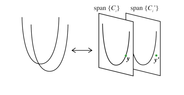
Figure 2: Proof of Lemma 14

Proof.

Let $B(0,1)$ denote the $\ell_{\infty}$ unit ball in $\mathbb{R}^{n}$. For every $x\in K_{C}\cap B(0,1)$,

$$\sum_{i\in[n]}C^{\prime}_{i}x_{i} =\sum_{i\in[n]}C_{i}x_{i}+\sum_{i\in[n]}(C_{i}-C^{\prime}_{i})x_{i}$$

$$\succeq-n\mathsf{mdist}(C,C^{\prime})\cdot\mathsf{Id}_{k}$$

where we are using the fact that $\sum_{i}C_{i}x_{i}\succeq 0$. This implies that the point $x^{\prime}=x+n\mathsf{mdist}(C,C^{\prime})\cdot\mathbf{1}\in K_{C^{\prime}}$. To see this, recall that the representation is normalized in that $\sum_{i}C^{\prime}_{i}=\mathsf{Id}_{k}$. Therefore, we get

$$\sum_{i}C^{\prime}_{i}x^{\prime}_{i}=\sum_{i}C^{\prime}_{i}x_{i}+n\cdot\mathsf{mdist}(C,C^{\prime})\sum_{i}C^{\prime}_{i}\succeq 0$$

The lemma follows by observing that $\|x-x^{\prime}\|_{2}\leq n^{3/2}\cdot\mathsf{mdist}(C,C^{\prime})$.

∎

6 Proof of The Main Theorem

We restate the theorem for convenience.

Theorem 15 (Restatement of Main Theorem).

There exists an absolute constant $\kappa>0$ such that for all sufficiently large $n,d$, there exists an n-variate degree $d$ hyperbolic polynomial $p$ whose hyperbolicity cone $K_{p}$ does not admit an $\eta-$approximate spectrahedral representation of dimension $B\leq\left(n/d\right)^{\kappa d}$, for $\eta=1/n^{4nd}$.

Proof.

Set $\epsilon$ smaller than $R$ and $R_{2}$. Theorem 5, Lemma 9 and Lemma 10 together imply a family of hyperbolic polynomials $\mathcal{P}$ with the following properties:

1. $|\mathcal{P}|=2^{|\mathcal{M}_{d}|}$ where $|\mathcal{M}_{d}|\geq(n/d)^{\kappa d}$ for some absolute constant $\kappa>0$.

2. For all $p\neq p^{\prime}\in\mathcal{P}$, $\mathsf{hdist}(K_{p},K_{p}^{\prime})\geq\gamma$ for $\gamma>\frac{1}{n^{3nd}}$.

3. For every $p\in\mathcal{P}$, the positive orthant $\mathbb{R}_{+}^{n}$ is contained in $K_{p}$.

The last observation follows from the fact that positive orthant is contained in $K_{e_{d}}$, and the perturbations of $e_{d}$ in $\mathcal{P}$ are small enough to keep all the coefficients non-negative.

Suppose each of the hyperbolicity cones $K_{p}$ admitted a $\gamma/3-$approximate spectrahedral representation in dimension $B$. By Lemma 13, for each cone in $K_{p}$, there exists a normalized $\gamma/3$-approximate spectrahedral representation $C_{p}$ in dimension $B_{p}\leq B$ Further, by Lemma 14, for every pair of polynomials $p,p^{\prime}\in\mathcal{P}$, their corresponding $\gamma/3$-approximate spectrahedral representations satisfy $\mathsf{mdist}(C_{p},C_{p^{\prime}})\geq n^{-3/2}\gamma/3\coloneqq\eta$.

Notice that in every normalized spectrahedral representation $C_{p}$ in dimension $B$, every matrix $C\in C_{p}$ satisfies $C\succeq 0$ and $C\preceq\mathsf{Id}_{B}$. This implies that $\|C\|_{F}\leq\sqrt{B}$. By a simple volume argument, for every $\eta>0$, the number of normalized spectrahedral representations in $\mathbb{R}^{B\times B}$ whose pairwise distances are $\geq\eta$ is at most $\left(\sqrt{B}/\eta\right)^{nB^{2}}$. Since every cone $K_{p}$ for $p\in\mathcal{P}$ admits a normalized spectrahedral representation of dimension at most $B$, we get that

$$|\mathcal{P}|\leq t\left(\sqrt{B}/\eta\right)^{nB^{2}}\ ,$$

which implies that

$$B^{2}\log B\geq|\mathcal{M}_{d}|/\log(n^{3/2}/\gamma)\geq\frac{1}{n\log n}\cdot(n/d)^{\kappa d}\ .$$

which implies the lower bound of $B\geq(n/d)^{\kappa^{\prime}d}$ for some constant $\kappa^{\prime}>0$. ∎

Acknowledgments

We thank Jim Renegar for pointing out a mistake in a previous version of the proof of Lemma 6. We thank the Simons Institute for the Theory of Computing and MSRI, where this work was partially carried out, for their hospitality.

Appendix

Proof of Lemma 11.

Let $z_{1}\leq,\ldots,\leq z_{d}=\lambda$ be the roots of $J(t)$. Observe that

$$J^{\prime}(\lambda)=\prod_{i<d}(z_{d}-z_{i})\geq|z_{d}-z_{d-1}|^{d-1},$$

so if we can prove a lowerbound on the spacing between $z_{d}$ and $z_{d-1}$ we are done.

We do this by recalling from Lemma 5 that:

$$J(t)=\frac{1}{d!}D^{n-d}t^{n-d}(1+t)^{d}.$$

Let $q_{k}(t):=D^{k}t^{n-d}(1+t)^{d}$ and note that $q_{k+1}$ interlaces $q_{k}$, and all of these polynomials have real roots in $[-1,0]$. Let $y_{k}$ be the largest root of $q_{k}$ that is strictly less than $0$, noting that every $q_{k}$ for $k<{n-d}$ has a root at $0$ because $q_{0}$ has a root of multiplicity $n-d$ at $0$. By lemma 8, we have for $k=1,\ldots,n-d$:

$$y_{k+1}\leq 0-\frac{1}{n}|0-y_{k}|\leq-|y_{k}|/n.$$

Noting that $y_{0}=-1$ and iterating this bound $n-d-1$ times we obtain

$$y_{n-d-1}\leq-1/n^{n-d-1},$$

so that $D^{n-d-1}q_{0}$ has a root at zero and a root $y_{n-d-1}\leq-1/n^{n-d}.$ Since $J(t)=Dq_{n-d-1}(t)$, we must have $z_{d-1}\leq-y_{n-d-1}$ by interlacing. However, applying Lemma 8 once more, we see that

$$z_{d}\geq-y_{n-d-1}+|0+y_{n-d-1}|/n=-(1-1/n)y_{n-d-1},$$

so the gap must be at least

$$z_{d}-z_{d-1}\geq y_{n-d-1}/n=\frac{1}{n^{n-d}}.$$

Thus, we conclude that

$$J^{\prime}(\lambda)\geq\frac{1}{n^{(d-1)(n-d)}}\geq\frac{1}{n^{d(n-d)}},$$

as desired. ∎

References

- [Ami16] Nima Amini, Spectrahedrality of hyperbolicity cones of multivariate matching polynomials, arXiv preprint arXiv:1611.06104 (2016).
- [Brä11] Petter Brändén, Obstructions to determinantal representability, Advances in Mathematics 226 (2011), no. 2, 1202–1212.
- [Brä14] , Hyperbolicity cones of elementary symmetric polynomials are spectrahedral, Optimization Letters 8 (2014), no. 5, 1773–1782.
- [COSW04] Young-Bin Choe, James G Oxley, Alan D Sokal, and David G Wagner, Homogeneous multivariate polynomials with the half-plane property, Advances in Applied Mathematics 32 (2004), no. 1-2, 88–187.
- [Går59] Lars Gårding, An inequality for hyperbolic polynomials, Journal of Mathematics and Mechanics 8 (1959), no. 6, 957–965.
- [Gül97] Osman Güler, Hyperbolic polynomials and interior point methods for convex programming, Mathematics of Operations Research 22 (1997), no. 2, 350–377.
- [HV07] J William Helton and Victor Vinnikov, Linear matrix inequality representation of sets, Communications on pure and applied mathematics 60 (2007), no. 5, 654–674.
- [LPR05] Adrian Lewis, Pablo Parrilo, and Motakuri Ramana, The lax conjecture is true, Proceedings of the American Mathematical Society 133 (2005), no. 9, 2495–2499.
- [Nui69] Wim Nuij, A note on hyperbolic polynomials, Mathematica Scandinavica 23 (1969), no. 1, 69–72.
- [Ren06] James Renegar, Hyperbolic programs, and their derivative relaxations, Foundations of Computational Mathematics 6 (2006), no. 1, 59–79.
- [San13] Raman Sanyal, On the derivative cones of polyhedral cones, Advances in Geometry 13 (2013), no. 2, 315–321.
- [Sau17] James Saunderson, A spectrahedral representation of the first derivative relaxation of the positive semidefinite cone, arXiv preprint arXiv:1707.09150 (2017).
- [SP15] James Saunderson and Pablo A Parrilo, Polynomial-sized semidefinite representations of derivative relaxations of spectrahedral cones, Mathematical Programming 153 (2015), no. 2, 309–331.
- [Zin08] Yuriy Zinchenko, On hyperbolicity cones associated with elementary symmetric polynomials, Optimization Letters 2 (2008), no. 3, 389–402.