Electromagnetically induced transparency and nonlinear pulse propagation in a combined tripod and $\Lambda$ atom-light coupling scheme

Abstract

We consider propagation of a probe pulse in an atomic medium characterized by a combined tripod and Lambda ($\Lambda$) atom-light coupling scheme. The scheme involves three atomic ground states coupled to two excited states by five light fields. It is demonstrated that dark states can be formed for such an atom-light coupling. This is essential for formation of the electromagnetically induced transparency (EIT) and slow light. In the limiting cases the scheme reduces to conventional $\Lambda$- or $N$-type atom-light couplings providing the EIT or absorption, respectively. Thus the atomic system can experience a transition from the EIT to the absorption by changing the amplitudes or phases of control lasers. Subsequently the scheme is employed to analyze the nonlinear pulse propagation using the coupled Maxwell-Bloch equations. It is shown that generation of stable slow light optical solitons is possible in such a five-level combined tripod and $\Lambda$ atomic system.

1 Introduction

Electromagnetically induced transparency (EIT) [1, 2, 3, 4, 5, 6] plays an important role in controlling the propagation of light puses in resonant media. Due to the EIT a weak probe beam of light tuned to an atomic resonance can propagate slowly and is almost lossless when the medium is driven by one or several control beams of light with a higher intensity [1, 2, 3, 4, 5, 6]. The EIT is formed because the control and probe beams drive the atoms to their dark states representing a special superposition of the atomic ground states immune to the atom-light coupling. The absorption is suppressed due to a quantum mechanical interference between different excitation pathways of atomic energy levels leading to the EIT. The EIT has various important applications in quantum and nonlinear optics, such as slow and stored light [7, 8, 9, 10, 11, 12], stationary light [13, 14], multiwave mixing [15, 16, 17], optical solitons [18, 19, 20, 21, 22, 23], optical bistability [24, 25] and Kerr nonlinearity [26, 27, 28, 29, 30]. Using the slow light greatly enhances the light-matter interaction and enables nonlinear optical processes to achieve significant efficiency even at a single- photon level [26, 31, 32, 33, 34, 35, 36, 37, 38].

There has been a considerable amount of activities on single- [39, 2, 12, 40, 41, 42, 8, 11, 3, 4, 43] and two-component (spinor) [44, 45, 46, 6, 47, 48] slow light in atomic media induced by the EIT. The former single-complonent slow light involves a probe beam of light and one or several control beams resonantly interacting with atomic media characterized by three level Lambda ($\Lambda$) type [2, 40] or four level tripod type [42, 49, 50, 41, 51] atom-light coupling schemes. In the later (spinor) case, double-tripod (DT) [44, 45, 46, 6, 47, 48] coupling schemes have been considered to support a simultaneous propagation of two probe beams leading to formation of a two-component slow light.

In this paper, we propose and analyze a novel five-level closed-loop scheme supporting the EIT. Closed-loop quantum configurations [52, 30, 45, 53, 54, 55] represent a class of atom-light coupling schemes in which the driving fields acting on atoms build closed paths for the transitions between atomic levels. The interference between different paths makes the system sensitive to relative phases of the applied fields. In our proposal illustrated in figure 1, the atom-light coupling represents a five-level combined Lambda-tripod scheme, in which three atomic ground states are coupled to two excited states by four control and one probe laser fields. In other words, the scheme involves four atomic levels coupled between each other by four control fields and interacting with a ground level through a weak probe field. The existence of dark states, essential for the EIT, is analytically demonstrated for such an atom-light coupling setup. It is shown that in some specific limiting cases this scheme can be equivalent to the conventional $\Lambda$- or $N$-type atom-light couplings. An advantage of such an atomic system is a possibility of transitions to the $\Lambda$ or $N$-type level schemes just by changing the amplitudes and phases of the control lasers. The limiting cases are discussed where the scheme reduces to atom-light couplings of the $\Lambda$- or $N$-type. By making a transition between the two limiting cases, one can switch from the EIT regime to the absorption for the probe field propagation.

Laser-driven atomic media, on the other hand, can be exploited to exhibit various nonlinear optical properties [15, 16, 18, 20, 24, 26, 31, 56, 57, 28, 58]. A particular example is formation of optical solitons with applications for optical buffers, phase shifters[59], switches[60], routers, transmission lines [61], wavelength converters [62], optical gates [63] and others. Solitons represent a specific type of stable shape-preserving waves propagating through nonlinear media. They can be formed due to a balance between dispersive and nonlinear effects leading to an undistorted propagation over long distance [64, 65, 63, 66, 67, 68, 69, 70, 71, 72, 73]. Following a report of ultraslow optical solitons in a highly resonant atomic medium by Wu and Deng [67], these solitary waves have received a considerable attention [74, 75, 76, 77, 22, 78, 79, 21, 80, 81, 19, 82, 23]. Here, the equations of motion that govern the nonlinear evolution of the probe-pulse envelope are derived for the Lambda-tripod atom-light coupling by solving the coupled Maxwell-Bloch equations. It is found that, by properly choosing the parameters of the system, the formation and slow propagation of shape-preserving optical solitons is feasible.

The paper is organized as follows. In section 2 we present the proposed setup and investigate propagation of the probe beam for various configurations of the control fields. Nonlinear propagation of the probe pulse is considered in section 3. Section 4 summarizes our findings.

2 Formulation and theoretical background

2.1 The system

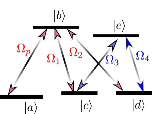
Figure 1: Schematic diagram of the five-level Lambda-tripod quantum system.

Let us consider a probe pulse described by a Rabi frequency $\Omega_{p}$. Additional laser fields described by Rabi frequencies $\Omega_{1},$ $\Omega_{2}$, $\Omega_{3}$ and $\Omega_{4}$ control propagation of the probe pulse. The probe and the control fields are assumed to co-propagate along the $z$ direction. We shall analyze the light-matter interaction in an ensemble of atoms using a five-level Lambda-tripod scheme shown in figure 1. The atoms are characterized by three ground levels $|a\rangle$, $|c\rangle$ and $|d\rangle$, as well as two excited states $|b\rangle$ and $|e\rangle$. Four coherent control fields with the Rabi frequencies $\Omega_{1},$ $\Omega_{2}$, $\Omega_{3}$ and $\Omega_{4}$ induce dipole-allowed transitions $|b\rangle\longleftrightarrow|c\rangle$, $|b\rangle\longleftrightarrow|d\rangle$, $|e\rangle\longleftrightarrow|c\rangle$, and $|e\rangle\longleftrightarrow|d\rangle$, respectively. As a result, the control fields couple two excited states $|b\rangle$ and $|e\rangle$ via two different pathways $|b\rangle\stackrel{{\scriptstyle\Omega_{1}^{*}}}{{\rightarrow}}|c\rangle\stackrel{{\scriptstyle\Omega_{3}}}{{\rightarrow}}|e\rangle$ and $|b\rangle\stackrel{{\scriptstyle\Omega_{2}^{*}}}{{\rightarrow}}|d\rangle\stackrel{{\scriptstyle\Omega_{4}}}{{\rightarrow}}|e\rangle$ making a four level closed-loop coherent coupling scheme described by the Hamiltonian ($\hbar=1$)

$$H_{\mathrm{4Levels}}=-\Omega_{1}^{*}|c\rangle\langle b|-\Omega_{2}^{*}|d\rangle\langle b|-\Omega_{3}^{*}|c\rangle\langle e|-\Omega_{4}^{*}|d\rangle\langle e|+\mathrm{H.c.}\,.$$ (1)

Furthermore, the tunable probe field with the Rabi frequency $\Omega_{p}$ induces a dipole-allowed optical transition $|a\rangle\longleftrightarrow|b\rangle$. The total Hamiltonian of the system involving all five atomic levels of the combined $\Lambda$ and tripod level scheme is given by

$$H_{\mathrm{5Levels}}=-\left(\Omega_{p}^{*}|a\rangle\langle b|+\Omega_{p}|b\rangle\langle a|\right)+H_{\mathrm{4Levels}}\,.$$ (2)

Note that the complex Rabi frequencies of the four control fields can be written as $\Omega_{j}=|\Omega_{j}|e^{i\phi_{i}}$, with $j=1,2,3,4$, where $|\Omega_{j}|$ and $\phi_{j}$ are the amplitude and phase of each applied field. As it will be explored below, in this scheme the destructive interference between different transition pathways induced by the the control and probe beams can make the medium transparent for the resonant probe beams in a narrow frequency range due to the EIT. We define $\phi=(\phi_{1}-\phi_{2})-(\phi_{3}-\phi_{4})$ to be a relative phase among the four control fields forming a closed-loop coherent coupling. By changing $\phi$, one can substantially modify the transparency and absorption properties for the probe field in such a Lambda-tripod scheme.

2.2 Equations of motion

The dynamics of the probe field propagating through the atomic medium is described by the Maxwell-Bloch equations. To the first-order of $\Omega_{p}$ the equations have the form

$$\dot{\rho}_{ba}^{(1)}=d_{1}\rho_{ba}^{(1)}+\rmi\Omega_{1}\rho_{ca}^{(1)}+\rmi\Omega_{2}\rho_{da}^{(1)}+\rmi\Omega_{p},$$ (3)

$$\dot{\rho}_{ca}^{(1)}=d_{2}\rho_{ca}^{(1)}+\rmi\Omega_{1}^{*}\rho_{ba}^{(1)}+\rmi\Omega_{3}^{*}\rho_{ea}^{(1)},$$ (4)

$$\dot{\rho}_{da}^{(1)}=d_{2}\rho_{da}^{(1)}+\rmi\Omega_{2}^{*}\rho_{ba}^{(1)}+\rmi\Omega_{4}^{*}\rho_{ea}^{(1)},$$ (5)

$$\dot{\rho}_{ea}^{(1)}=d_{3}\rho_{ea}^{(1)}+\rmi\Omega_{3}\rho_{ca}^{(1)}+\rmi\Omega_{4}\rho_{da}^{(1)},$$ (6)

and

$$\frac{\partial\Omega_{p}}{\partial z}+c^{-1}\frac{\partial\Omega_{p}}{\partial t}=\rmi\eta\rho_{ba}^{(1)}\,,\quad\mathrm{with}\quad\eta=\frac{2N\omega_{p}|\mu_{ba}|^{2}}{\hbar c}\,,$$ (7)

where $\rho_{u,v}^{(1)}$ are the first-order matrix elements of the density materix operator $\rho=\sum|u\rangle\rho_{uv}\langle v|$. The optical Bloch equations (3)–(6) imply the probe field to be much weaker than the control ones. In that case most atomic population is in the ground state $|a\rangle$, and one can treat the probe field as a perturbation. Therefore, we can apply the perturbation expansion $\rho_{ij}=\Sigma_{k}\rho_{ij}^{(k)},$ where $\rho_{ij}^{(k)}$ represents the $k$th order part of $\rho_{ij}$ in terms of probe field $\Omega_{p}$. Since $\Omega_{p}\ll\Omega_{i}$ $(i=1,2,3,4)$, the zeroth-order solution is $\rho_{aa}^{(0)}=1$, while other elements being zero ($\rho_{bb}^{(0)}=\rho_{cc}^{(0)}=\rho_{dd}^{(0)}=\rho_{ee}^{(0)}=0$). All fast-oscillating exponential factors associated with central frequencies and wave vectors have been eliminated from the equations, and only the slowly-varying amplitudes are retained.

The wave equation (7) describes propagation of the probe field $\Omega_{p}$ influenced by the atomic medium, where $\mu_{ba}$ is an electric dipole matrix element corresponding to the transition $|b\rangle\longleftrightarrow|a\rangle$, $N$ is the atomic density and $\omega_{p}$ is the frequency of the probe field. The density matrix equations (3)–(6) describe the evolution of the atomic system affected by the control and probe fields. They follow from the general quantum Liouville equation for the density matrix operator [83]

$$\dot{\rho}=-\frac{\rmi}{\hbar}[H_{\mathrm{5Levels}},\rho]+L_{\rho},$$ (8)

where the damping operator $L_{\rho}$ describes the decay of the system described by parameters $d_{1}=-\Gamma_{b}/2+\rmi\Delta_{p}$, $d_{2}=\rmi(\Delta_{p}-\Delta_{2})$ and $d_{3}=-\Gamma_{e}/2+\rmi(\Delta_{p}+\Delta_{3}-\Delta_{2})$ in equations (3)–(6). We have defined the detunings as: $\Delta_{2}=\Delta_{bc}=\Delta_{bd},$ and $\Delta_{3}=\Delta_{ec}=\Delta_{ed}$, with $\Delta_{bc}=\omega_{1}-\omega_{bc}$, $\Delta_{bd}=\omega_{2}-\omega_{bd}$, $\Delta_{ec}=\omega_{3}-\omega_{ec}$, $\Delta_{ed}=\omega_{4}-\omega_{ed}$, and $\Delta_{p}=\omega_{p}-\omega_{ba}$, where $\omega_{i}$ is a central frequency of the corresponding control field. Two excited states $\left|b\right\rangle$ and $\left|e\right\rangle$ decay with rates $\Gamma_{b}$ and $\Gamma_{e}$, respectively.

2.3 Transition to a new basis

The Hamiltonian for the atomic four-level subsystem (1) can be represented as

$$H_{\mathrm{4Levels}}=-\beta|D_{e}\rangle\langle b|-\alpha|B_{e}\rangle\langle b|-\Omega|B_{e}\rangle\langle e|+\mathrm{H.c.},$$ (9)

where

$$|D_{e}\rangle=\frac{1}{\Omega}\left(\Omega_{4}|c\rangle-\Omega_{3}|d\rangle\right),$$ (10)

$$|B_{e}\rangle=\frac{1}{\Omega}\left(\Omega_{3}^{*}|c\rangle+\Omega_{4}^{*}|d\rangle\right)$$ (11)

are the internal dark and bright states for the $\Lambda$- scheme made of the two ground states states $|c\rangle$ and $|d\rangle$, as well as an excited states $|e\rangle$. One can also introduce another set of dark and bright states corresponding to the $\Lambda$- scheme made of the same pair of ground states states $|c\rangle$ and $|d\rangle$, yet a different excited state $|b\rangle$:

$$|D_{b}\rangle=\frac{1}{\Omega}\left(\Omega_{2}|c\rangle-\Omega_{1}|d\rangle\right),$$ (12)

$$|B_{b}\rangle=\frac{1}{\Omega}\left(\Omega_{1}^{*}|c\rangle+\Omega_{2}^{*}|d\rangle\right).$$ (13)

In writing equation (9), the coefficient

$$\beta=\langle D_{b}|B_{e}\rangle=\langle D_{e}|B_{d}\rangle=\frac{1}{\Omega}(\Omega_{1}^{*}\Omega_{4}^{*}-\Omega_{2}^{*}\Omega_{3}^{*})$$ (14)

represents the quantum inteference between the four control fields playing the main role in tuning dispersion and absorption properties in the combined tripod and $\Lambda$ scheme. In addition, we define

$$\alpha=\langle D_{b}|D_{e}\rangle=\langle B_{e}|B_{d}\rangle=\frac{1}{\Omega}(\Omega_{1}^{*}\Omega_{3}+\Omega_{2}^{*}\Omega_{4})$$ (15)

and the total Rabi frequency

$$\Omega=\sqrt{|\Omega_{3}|^{2}+|\Omega_{4}|^{2}}\,.$$ (16)

By changing the quantum interference coefficient $\beta$ and the coefficient $\alpha$ one arrives at three different situations. For each of them we shall plot the level schemes in the basis involving the transformed states $|B_{e}\rangle$ and $|D_{e}\rangle$.

2.3.1 Situation (a): $\beta\neq 0$ and $\alpha\neq 0$

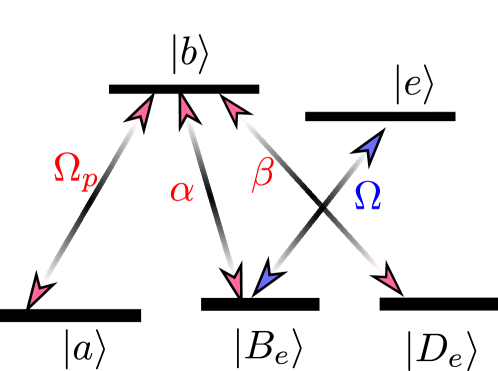
Figure 2: Five-level quantum system in the transformed basis for $\beta\neq 0$ and $\alpha\neq 0$.

In the case when both coefficients $\alpha$ and $\beta$ are nonzero, the five-level tripod and $\Lambda$ scheme shown in figure 2 looks similar to the original scheme (figure 1) in the transformed basis, but the coupling between the states $|D_{e}\rangle$ and $|e\rangle$ is missing. The coefficient $\beta$ is nonzero when $\Omega_{1}\Omega_{4}\neq\Omega_{2}\Omega_{3}$. The condition $\beta\neq 0$ is valid provided $|\Omega_{1}||\Omega_{4}|\neq|\Omega_{2}||\Omega_{3}|$ and phase $\phi$ is arbitrary, or $|\Omega_{1}||\Omega_{4}|=|\Omega_{2}||\Omega_{3}|$ with $\phi\neq 0$.

When both $\alpha$ and $\beta$ are nonzero, one can define a global dark state $|D\rangle$ for the whole atom-light coupling scheme

$$|D\rangle=\beta|a\rangle-\Omega_{p}|D_{e}\rangle\,.$$ (17)

The dark state is an eigenstate of the full atom-light Hamiltonian with a zero eigen-energy: $H_{\mathrm{5Levels}}|D\rangle=0$. The state $|D\rangle$ has no contribution by the ground state superpositon $|B_{e}\rangle$, as well as no contribution by the bare excited states $|e\rangle$ and $|b\rangle$. As a result, there is no transition from the state $|D\rangle$ to the excited states $|e\rangle$ and $|b\rangle$, making the five-level closed- loop scheme transparent to the electromagnetic field. This is a new mechanism for the EIT compared with the $\Lambda$ [2, 8], tripod [42, 41], or double tripod schemes [45, 46].

It is known that the real and imaginary parts of $\rho_{ba}^{(1)}$ correspond to the probe dispersion and absorption, respectively. A steady-state solution to the density matrix element $\rho_{ba}$ reads under the resonance condition $\Delta_{2}=\Delta_{3}=0$

$$\rho_{ba}^{(1)}=\Omega_{p}\Delta_{p}(|\Omega_{3}|^{2}+|\Omega_{4}|^{2}+\rmi\Delta_{p}(-\Gamma_{e}/2+\rmi\Delta_{p}))$$

$$\times\left[|\beta|^{2}\Omega^{2}+\rmi\Delta_{p}(-\Gamma_{e}/2+\rmi\Delta_{p})(|\Omega_{1}|^{2}+|\Omega_{2}|^{2})\right.$$

$$+\left.\rmi\Delta_{p}(-\Gamma_{b}/2+\rmi\Delta_{p})\left(|\Omega_{3}|^{2}+|\Omega_{4}|^{2}+\rmi\Delta_{p}(-\Gamma_{e}/2+\rmi\Delta_{p})\right)\right]^{-1},$$ (18)

where the interference term $\beta$ is involved.

A denominator of equation (18) represents the fourth order polynomial which contains zero points at four different detunings $\Delta_{p}$ of the probe field from the EIT resonance. This provides four maxima in the absorption profile of the system, as one can see in figure 5(a). Furthermore the EIT window is formed for zero detuning. In A we have presented eigenstates and the corresponding eigenvalues of the Hamiltonian (9) describing the four-level subsystem. One can see that all four eigenstates $|n_{i}\rangle$ characterized by the eigenvalues $\lambda_{1,2}=\mp\frac{\sqrt{S-Y}}{\sqrt{2}}$ and $\lambda_{3,4}=\mp\frac{\sqrt{S+Y}}{\sqrt{2}}$ contain contributions due to the excited state $|b\rangle$ (note that $S$ and $Y$ can be found in A). This results in four peaks in absorption profile of the system.

2.3.2 Situation (b): $\beta=0$ and $\alpha\neq 0$

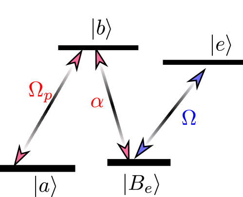
Figure 3: The level scheme in the transformed basis for $\beta=0$ and $\alpha\neq 0$. The ground state superposition $|D_{e}\rangle$ (now shown in the figure) is decoupled from the remaining four states.

The condition $\beta=0$ is fulfilled if $\Omega_{1}\Omega_{4}=\Omega_{2}\Omega_{3}$, or equivalently $|\Omega_{2}||\Omega_{3}|=|\Omega_{1}||\Omega_{4}|$ and $\phi=0$. In that case the state $|D_{e}\rangle$ is not involved, so the interaction Hamiltonian (9) for the four-level subsystem can be rewritten as

$$H_{\mathrm{4Levels}}=-\alpha|B_{e}\rangle\langle b|-\Omega|B_{e}\rangle\langle e|+\mathrm{H.c.}\,.$$ (19)

Consequently the five-level tripod and $\Lambda$ scheme becomes equivalent to a conventional $N$-type atomic system [29, 84] shown in figure 3.

Since the quantum interference term $\beta$ vanishes, equation (18) simplifies to

$$\rho_{ba}^{(1)}=\Omega_{p}(|\Omega_{3}|^{2}+|\Omega_{4}|^{2}+\rmi\Delta_{p}(-\Gamma_{e}/2+\rmi\Delta_{p}))$$

$$\times\left[\rmi(-\Gamma_{e}/2+\rmi\Delta_{p})(|\Omega_{1}|^{2}+|\Omega_{2}|^{2})\right.$$

$$+\left.\rmi(-\Gamma_{b}/2+\rmi\Delta_{p})(|\Omega_{3}|^{2}+|\Omega_{4}|^{2}+\rmi\Delta_{p}(-\Gamma_{e}/2+\rmi\Delta_{p}))\right]^{-1}.$$ (20)

The denominator of $\rho_{ba}^{(1)}$ in equation (20) is now a cubic polynomial, providing three absorption maxima. The eigenstates and eigenvalues corresponding to this situation are presented in B. The eigenvector $|n_{2}\rangle$ characterized by a zero eigen-energy coincides with the dark state $|D_{e}\rangle$ and is decoupled from the radiation fields. Only the remaining three eigenvectors $|n_{1}\rangle$, $|n_{3}\rangle$ and $|n_{4}\rangle$ contain the contribution due to an excited state $|b\rangle$. This leads to three absorption peaks displayed in figure 5(b). In this way, the absence of quantum interference term $\beta$ between the control fields destroys one of the peaks in the absorption profile leading to three absorption maxima.

2.3.3 Situation (c): $\beta\neq 0$ and $\alpha=0$

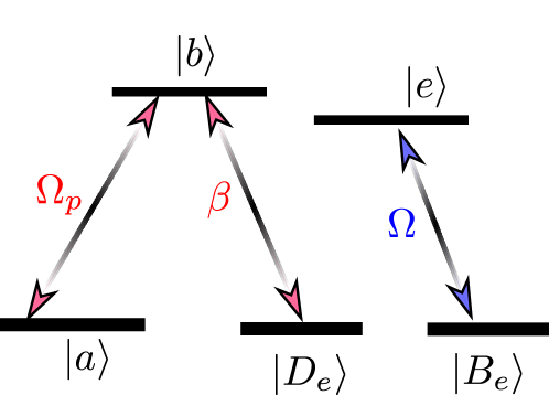
Figure 4: Schematic diagram of the five-level quantum system for $\beta\neq 0$ and $\alpha=0$.

When the coefficient $\beta$ is nonzero but the coefficient $\alpha$ is zero, the interaction Hamiltonian (9) can be represented as

$$H_{\mathrm{4Levels}}=-\beta|D_{e}\rangle\langle b|-\Omega|B_{e}\rangle\langle e|+\mathrm{H.c.}\,.$$ (21)

As illustrated in figure 4, the five-level tripod and $\Lambda$ scheme is then equivalent to a conventional $\Lambda$-type atomic system [2, 40] which is decoupled from the two-level system involving the states $|B_{e}\rangle$ and $|e\rangle$.

In the following we consider a symmetric case where $|\Omega_{1}|=|\Omega_{2}|$, $|\Omega_{3}|=|\Omega_{4}|$ and $\phi=\pi$. In such a situation the conditions $\beta\neq 0$ and $\alpha=0$ are fulfilled, with $\beta^{2}=2|\Omega_{1}^{2}|$. Equation (18) for $\rho_{ba}$ then simplifies considerably, giving

$$\rho_{ba}^{(1)}=\Omega_{p}\frac{\Delta_{p}}{|\beta|^{2}+\rmi\Delta_{p}\left(-\frac{\Gamma_{b}}{2}+\rmi\Delta_{p}\right)}\,.$$ (22)

Obviously, the polynominal in denominator becomes quadratic in $\Delta_{p}$ resulting in two absorption peaks or a single EIT window, which is a characteristic feature of the $\Lambda$ scheme. Furthermore, the probe absorption and dispersion do not dependent on $\Omega$, only $\beta$ contributes to the optical properties. This is because the $\Lambda$-type scheme is now decoupled from the transition $|B_{e}\rangle\stackrel{{\scriptstyle\Omega}}{{\rightarrow}}|e\rangle$, and the system behaves as a three- level $\Lambda$-type scheme containing $|a\rangle,$ $|b\rangle$, and $|D_{e}\rangle$.

In the following we summarize our results for the behavior of real and imaginary parts of $\rho_{ba}^{(1)}$ corresponding to the probe dispersion and absorption for different situations (a)–(c) described above. Without a loss of generality, in all the simulations we take $\Gamma_{e}=\Gamma_{b}=\gamma$. The other frequencies are scaled by $\gamma$ which should be in the order of MHz for cesium (Cs) atoms. Figure 5 shows that the our model provides a high control of dispersive-absorptive optical properties of the probe field. The absorption profile has four, three and two peaks featured in figures 5(a)–5(c), respectively. There is the resulting change in the sign of the slope of the dispersion at $\Delta_{p}=0$ for different situations (a)–(c). This gives rise to switching in the group velocity of the probe pulse from subluminal to superluminal or visa versa. In particular, for the choice of parameters satisfying situation (a) and (c), there is the subluminality accompanied by EIT at line center. On the other hand, the superluminality accompanied by a considerable absorption is observed for the parametric condition satisfying the situation (b).

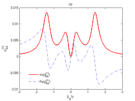
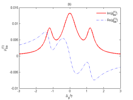
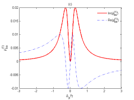
Figure 5: Probe absorption ($\mathrm{Im}(\rho_{ba}^{(1)}$)) versus $\Delta_{p}$ for (a) $\Omega_{1}=0.9\gamma$, $\Omega_{2}=0.7\gamma$, $\Omega_{3}=0.4\gamma$, $\Omega_{4}=0.8\gamma$, and $\phi=0$ corresponding to the first situation, (b) $\Omega_{1}=\Omega_{2}=0.5\gamma$, $\Omega_{3}=\Omega_{4}=0.7\gamma$ and $\phi=0$ corresponding to the second situation, and (c) $\Omega_{1}=\Omega_{2}=0.2\gamma$, $\Omega_{3}=\Omega_{4}=0.1\gamma$ and $\phi=\pi$ corresponding to the third situation. Other parameters are $\Gamma_{e}=\Gamma_{b}=\gamma$, $\Delta_{2}=\Delta_{3}=0$, and $\Omega_{p}=0.01\gamma$. Note that all frequencies are scaled by $\gamma$ which should be in the order of MHz, like for cesium (Cs) atoms.

3 Linear and nonlinear pulse propagation in combined tripod and $\Lambda$ scheme

In this section we consider propagation of the probe pulse in the proposed tripod and $\Lambda$ scheme. Performing the time Fourier transform of equations (3)–(7) one can obtain

$$t_{1}(\omega)F_{ba}+\Omega_{1}F_{ca}+\Omega_{2}F_{da}+\Lambda_{p}=0,$$ (23)

$$t_{2}(\omega)F_{ca}+\Omega_{1}^{*}F_{ba}+\Omega_{3}^{*}F_{ea}=0,$$ (24)

$$t_{2}(\omega)F_{da}+\Omega_{2}^{*}F_{ba}+\Omega_{4}^{*}F_{ea}=0,$$ (25)

$$t_{3}(\omega)F_{ea}+\Omega_{3}F_{ca}+\Omega_{4}F_{da}=0,$$ (26)

and

$$\frac{\partial\Lambda_{p}}{\partial z}-\rmi\frac{\omega}{c}\Lambda_{p}=\rmi\eta F_{ba},$$ (27)

where $t_{1}(\omega)=\omega+i\Gamma_{b}/2+\Delta_{p}$, $t_{2}(\omega)=\omega+\Delta_{p}-\Delta_{2}$, and $t_{3}(\omega)=\omega+\rmi\Gamma_{e}/2+\Delta_{p}-\Delta_{2}+\Delta_{3}$. Note that $F_{ij}$ and $\Lambda_{p}$ represent the Fourier transforms of $\rho_{ij}^{(1)}$ and $\Omega_{p}$, respectively, where $\omega$ is a deviation from the central frequency.

A solution of equation (27) is a plane wave of the form

$$\Lambda_{p}(z,\omega)=\Lambda_{p}(0,\omega)\rme^{\rmi\kappa(\omega)z},$$ (28)

where

$$\kappa=\frac{\omega}{c}-\frac{\eta S_{1}(\omega)}{Q(\omega)},$$ (29)

describes the linear dispersion relation of the system. Expanding $\kappa$ in power series around the center frequency of the probe pulse ($\omega=0$) and taking only the first three terms, we get

$$\kappa=\kappa_{0}+\kappa_{1}\omega+\kappa_{2}\omega^{2},$$ (30)

where the detaied expressions for the coefficients $\kappa_{0}$, $\kappa_{1}$ and $\kappa_{2}$ are given in C, while $S_{1}(\omega)$ and $Q(\omega)$ can be found in D. In equation (30), $\kappa_{i}=\frac{d^{j}\kappa(\omega)}{d\omega^{j}}|_{\omega=0}$ with $j=0,1,2$ are the dispersion coefficients in different orders. In general, the real part of $\kappa_{0}=\Upsilon+\rmi\chi/2$ defines the phase shift $\Upsilon$ per unit length, while the imaginary part indicates the linear absorption $\chi$ of the probe pulse. The group velocity $v_{g}$ is given by $1/\kappa_{1}$, whereas the quadratic term $\kappa_{2}$ is associated with the group velocity dispersion which causes the pulse distortion.

In the linear regime, we take an incoming probe pulse to be of the Gausian shape, $\Omega_{p}(0,t)=\Omega_{p}^{0}\rme^{-(t/\tau_{0})^{2}}$, with a duration $\tau_{0}$. The subsequent time evolution is obtained from equation (28) by carrying out an inverse Fourier transform [67]

$$\Omega_{p}(z,t)=\frac{\Omega_{p}^{0}}{\sqrt{L_{z}}}\exp\left[\rmi\kappa_{0}z-\frac{(t-\kappa_{1}z)^{2}}{L_{z}\tau_{0}^{2}}\right]\,,$$ (31)

with $L_{z}=s_{1}(z)-\rmi s_{2}(z)$, $s_{1}(z)=1+4z\mathrm{Re}(\kappa_{2})/\tau_{0}^{2}$ and $s_{2}(z)=4z\mathrm{Im}(\kappa_{2})/\tau_{0}^{2}$ . In this way, even if there is no absorption due to EIT ($\mathrm{Im}(\kappa_{i})=0$, $i=0,1,2$), the dispersion effects can contribute to the pulse attenuation and spreading during propagation.

Our goal is to obtain shape-preserving optical pulses which can propagate without significant distortion and loss in our medium. The idea is to include the optical Kerr nonlinearity of the probe laser field into the light propagation, and show that the Kerr nonlinear effect can compensate the dispersion effects and result in shape-preserving optical pulses. To balance the dispersion effects and optical nonlinearity, in the following a theoretical model is employed based on the coupled Maxwell-Bloch equations for the nonlinear pulse propagation. Following [67], we take a trial function

$$\Lambda_{p}=\tilde{\Lambda}_{p}\rme^{\rmi\kappa_{0}z}\,.$$ (32)

Substituting equation (32) into the wave equation (27) and using equations (29), (30) and (64) we obtain

$$\frac{\partial\Lambda_{p}}{\partial z}\rme^{\rmi\kappa_{0}z}=\rmi(\kappa_{1}\omega+\kappa_{2}\omega^{2})\Lambda_{p}\rme^{\rmi\kappa_{0}z},$$ (33)

where we have replaced $\tilde{\Lambda}_{p}$ with $\Lambda_{p}$ for the sake of convenience. Here we only keep terms up to the order $\omega^{2}$ in expanding the dispersion relarion $\kappa_{j}$.

In deriving the linearized wave equation (7), the nonlinear polarization due to the optical Kerr nonlinearity of the probe field has been neglected. Now we turn to investigate the nonlinear propagation of light due to the Kerr effect. To incorporate the nonlinear optical terms in the pulse propagation, the right hand side of wave equation (7) must be rewritten as $\rmi\eta\rho_{ba}^{(1)}-\rmi\eta\mathrm{Kerr}$. The Kerr nonlinear term has an opposite sign than the linear term $\rmi\eta\rho_{ba}^{(1)}$ and the probe absorption and dispersion are proportional to imaginary and real parts of $\rho_{ba}^{(1)}$, respectively. Consequently a large optical nonlinearity can cancel the dispersion and suppress the absorption of probe field, effectively. A derivation of the Kerr nonlinear coefficient is provided in E.

Performing the inverse Fourier transform of equation (33), using the expression (83) for $\mathrm{Kerr}$ and introducing new coordinates $\zeta=z,$ and $\eta=t-z/v_{g},$ we arrive at the nonlinear wave equation for the slowly varing envelope $\Omega_{p}$

$$\rmi\frac{\partial}{\partial\zeta}\Omega_{p}-\kappa_{2}\frac{\partial^{2}}{\partial\eta^{2}}\Omega_{p}=\Theta\rme^{-\chi\zeta}|\Omega_{p}|^{2}\Omega_{p}.$$ (34)

where $\Theta=-\eta\mathrm{Kerr}$, and $\chi=2\mathrm{Im}(\kappa_{0})=2\eta\mathrm{Im}\left(\frac{-S_{1}}{Q}\right)$.

Equation (34) contains generally complex coefficients. However, for suitable set of system parameters, the absorption coefficent $\chi$ may be very small, i.e., $\chi\simeq 0$, and imaginary parts of coefficients $\Theta$ and $K_{2}$ may be made very small in comparison to their real parts, i.e., $\kappa_{2}=\kappa_{2r}+\rmi\kappa_{2i}\approx\kappa_{2r}$, and $\Theta=\Theta_{r}+\rmi\Theta_{i}\approx\Theta_{r}$. In this case equation (34) can be written as

$$\rmi\frac{\partial}{\partial\zeta}\Omega_{p}-\kappa_{2r}\frac{\partial^{2}}{\partial\eta^{2}}\Omega_{p}=\Theta_{r}|\Omega_{p}|^{2}\Omega_{p}.$$ (35)

This represents the conventional nonlinear Schrodinger (NLS) equation which describes the nonlinear evolution of the probe pulse and allows bright and dark soliton solutions. The nature of the soliton solution is determined by a sign of the product $\kappa_{2r}\Theta_{r}$. A bright soliton is obtained for $\kappa_{2r}\Theta_{r}>0$, and the solution is then given by

$$\Omega_{p}=\Omega_{p0}\mathrm{sech}(\eta/\tau)\exp\left(-\rmi\zeta\Theta_{r}|\Omega_{p}|^{2}/2\right)\,.$$ (36)

For $\kappa_{2r}\Theta_{r}<0$, one obtains the dark solion solution of the form

$$\Omega_{p}=\Omega_{p0}\mathrm{tanh}(\eta/\tau)\exp\left(-\rmi\zeta\Theta_{r}|\Omega_{p}|^{2}/2\right)\,.$$ (37)

Here $\Omega_{p0}=(1/\tau)\sqrt{|\kappa_{2r}/\Theta_{r}|}$ represents an amplitude of the probe field and $\tau$ is the typical pulse duration (soliton width).

In the following, we explore a possibility for the formation of the shape preserving optical solitons in this combined tripod and $\Lambda$ scheme for a realistic atomic system and present numeric calculations. The proposed scheme involving the five-level combined tripod and $\Lambda$ structure can be experimentally implemented using the cesium (Cs) atom vapor. In our proposal, the levels $|c\rangle$, $|d\rangle$ and $|e\rangle$ can correspond to $|6S_{1/2},F=3,M_{F}=+1\rangle$, $|6S_{1/2},F=3,M_{F}=+3\rangle$ and $|6P_{3/2},F=2,M_{F}=+2\rangle$, respectively. In addition, the levels $|b\rangle$ and $|a\rangle$ can correspond to $|6P_{3/2},F=4\rangle$ and $|6S_{1/2},F=4\rangle$, respectively. The two excited states are assumed to decay with the rates $\Gamma_{e}=\Gamma_{b}=\gamma=2\pi\times 5.2\,\mathrm{MHz}$.

Assuming the parameteric situation (a) described in the previous section, we take $|\Omega_{1}|=|\Omega_{2}|=1.97\times 10^{9}\,\mathrm{s}^{-1}$, $|\Omega_{3}|=2.3\times 10^{9}\,\mathrm{s}^{-1}$, $|\Omega_{4}|=16.4\times 10^{7}\,\mathrm{s}^{-1}$, $\Delta_{2}=6.4\times 10^{9}\,\mathrm{s}^{-1},$ $\Delta_{p}=5.9\times 10^{9}\,\mathrm{s}^{-1}$ and $\Delta_{3}=82\times 10^{7}\,\mathrm{s}^{-1}$. Consequentlhy we obtain $\kappa_{0}\approx(3.9+0.008i)\,\mathrm{cm}^{-1}$, $\kappa_{1}\approx(4.7-2.1\times 10^{-2}i)10^{-9}\,\mathrm{cm}^{-1}\cdot\mathrm{s}$, $\kappa_{2}\approx(-8.06-3.6\times 10^{-2}i)10^{-17}\,\mathrm{cm}^{-1}\cdot\mathrm{s}^{2}$, and $\Theta\approx(3.6-1.12\times 10^{-2}i)10^{-19}\,\mathrm{cm}^{-1}\cdot\mathrm{s}^{2}$. In this case, the standard nonlinear Schrodinger equation (35) with $\kappa_{2r}\Theta_{r}<0$ is well characterized, leading to the formation of dark solitons in the proposed system. With this set of parameters, the fundamental soliton has a width and amplitude satisfying $|\Omega_{p0}\tau|=\sqrt{\kappa_{2r}/\Theta_{r}}\simeq 4.7$. As shown in figure 6, the dark soliton of this type remains fairly stable during propagation, which is due to the balance between the group-velocity dispersion and Kerr-type optical nonlinearity. According to equation (58) in C, the group velocity $v_{g}$ has a general form $v_{g}^{-1}=c^{-1}+\eta(-g_{1}/Q+S_{1}g_{2}/Q^{2})$, with all coefficients given in C. With the above system parameters, one can find $v_{g}\approx 7\times 10^{-3}c,$ indicating that the soliton propagates with a slow velocity.

The formation and propagation of such a slow light optical soliton in the system is due to the EIT condition described in the situation (a) of the previous section, i.e., $\beta\neq 0$ and $\alpha\neq 0$, or equivalently $\Omega_{1}\Omega_{4}\neq\Omega_{2}\Omega_{3}$. Due to the EIT, the absorption of the probe field becomes negligibly small. In this case, an enhanced Kerr nonlinearity can compensate the dispersion effects in such a highly resonant medium resulting in shape preserving slow light optical solitons.

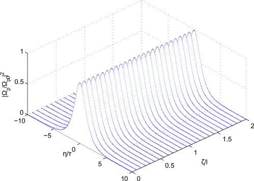
Figure 6: Propagation dynamics of an ultraslow optical soliton with $\tau=10^{-7}\,\mathrm{s}$, $l=1\,\mathrm{cm}$, and $\eta=1.0\times 10^{10}\,\mathrm{cm}^{-1}\cdot\mathrm{s}^{-1}$ and the parameters given in the main text.

4 Concluding Remarks

In conclusion we have demonstrated the existence of dark states which are essential for appearance of electromagnetically induced transparency (EIT) for a situation where the atom- light interaction represents a five-level combined tripod and $\Lambda$ configuration. The EIT is possible in the combined tripod and $\Lambda$ scheme when the Rabi frequencies of the control fields obey the condition $\beta\neq 0$, $\alpha\neq 0$, where $\beta$ and $\alpha$ given by equations (14)–(15) characterize the relative amplitudes and phases of the four control fields. Under this condition, the medium supports the lossless propagation of slow light. It is analytically demonstrated that combined tripod and $\Lambda$ scheme can reduce to simpler atom light-coupling configurations under various quantum interference situations. In particular, this scheme is equivalent to a four-level $N$-type scheme when $\beta=0$ and $\alpha\neq 0$. On the other hand, for $\beta\neq 0$ but $\alpha=0$, a three-level $\Lambda$-type atom-light coupling scheme can be established. As a result, by changing the Rabi frequencies of control fields, it is possible to make a transition from one limiting case to the another one. This can lead to switching from subluminality accompanied by EIT to superluminality along with absorption and visa versa. Based on the coupled Maxwell-Bloch equations, a nonlinear equation governing the evolution of the probe pulse envelope is then obtained. This leads to formation of stable optical solitons with a slow propagating velocity due to the balance between dispersion and Kerr nonlinearity of the system.

A possible realistic experimental realization of the proposed combined tripod and $\Lambda$ setup can be implemented for the Cs atoms. The lower levels $|a\rangle$, $|c\rangle$ and $|d\rangle$ can then be assigned to $|6S_{1/2},F=4\rangle$, $|6S_{1/2},F=3,M_{F}=+1\rangle$ and $|6S_{1/2},F=3,M_{F}=+3\rangle$, respectively. Two excited states $|b\rangle$and $|e\rangle$ can be attributed to the Cs states $|6P_{3/2},F=4\rangle$ and $|6P_{3/2},F=2,M_{F}=+2\rangle$, respectively.

Appendix A Eigenstates and eigenvalues for situation (a)

The expressions for the eigenstates and their corresponding eigenvalues for situaion (a) are:

$$|n_{1}\rangle=\frac{\alpha^{*}(S-Y)}{\Omega(X-Y)}|b\rangle-\frac{\sqrt{S-Y}}{\sqrt{2}\Omega}|B_{e}\rangle-\frac{\alpha^{*}\beta\sqrt{2(S-Y)}}{\Omega(X-Y)}|D_{e}\rangle+|e\rangle\,,$$ (38)

$$|n_{2}\rangle=\frac{\alpha^{*}(S-Y)}{\Omega(X-Y)}|b\rangle+\frac{\sqrt{S-Y}}{\sqrt{2}\Omega}|B_{e}\rangle+\frac{\alpha^{*}\beta\sqrt{2(S-Y)}}{\Omega(X-Y)}|D_{e}\rangle+|e\rangle\,,$$ (39)

$$|n_{3}\rangle=\frac{\alpha^{*}(S+Y)}{\Omega(X+Y)}|b\rangle-\frac{\sqrt{S+Y}}{\sqrt{2}\Omega}|B_{e}\rangle-\frac{\alpha^{*}\beta\sqrt{2(S+Y)}}{\Omega(X+Y)}|D_{e}\rangle+|e\rangle\,,$$ (40)

$$|n_{4}\rangle=\frac{\alpha^{*}(S+Y)}{\Omega(X+Y)}|b\rangle+\frac{\sqrt{S+Y}}{\sqrt{2}\Omega}|B_{e}\rangle+\frac{\alpha^{*}\beta\sqrt{2(S+Y)}}{\Omega(X+Y)}|D_{e}\rangle+|e\rangle\,,$$ (41)

with eigenvalues

$$\lambda_{1}=-\frac{\sqrt{S-Y}}{\sqrt{2}}\,,$$ (42)

$$\lambda_{2}=\frac{\sqrt{S-Y}}{\sqrt{2}}\,,$$ (43)

$$\lambda_{3}=-\frac{\sqrt{S+Y}}{\sqrt{2}}\,,$$ (44)

$$\lambda_{4}=\frac{\sqrt{S+Y}}{\sqrt{2}}\,,$$ (45)

where

$$S=|\alpha|^{2}+|\beta|^{2}+\Omega^{2}\,,$$ (46)

$$X=|\alpha|^{2}-|\beta|^{2}+\Omega^{2}\,,$$ (47)

$$Y=\sqrt{S^{2}-4|\beta|^{2}\Omega^{2}}\,.$$ (48)

Appendix B Eigenstates and eigenvalues for situation (b)

The expressions for the eigenstates and their corresponding eigenvalues for situaion (b) are:

$$|n_{1}\rangle=-\frac{\Omega}{\alpha}|b\rangle+|e\rangle\,,$$ (49)

$$|n_{2}\rangle=|D_{e}\rangle\,,$$ (50)

$$|n_{3}\rangle=\frac{\alpha^{*}}{\Omega}|b\rangle-\frac{\sqrt{|\alpha|^{2}+\Omega^{2}}}{\Omega}|B_{e}\rangle+|e\rangle\,,$$ (51)

$$|n_{4}\rangle=\frac{\alpha^{*}}{\Omega}|b\rangle+\frac{\sqrt{|\alpha|^{2}+\Omega^{2}}}{\Omega}|B_{e}\rangle+|e\rangle\,,$$ (52)

with eigenvalues

$$\lambda_{1}=0\,,$$ (53)

$$\lambda_{2}=0\,,$$ (54)

$$\lambda_{3}=-\sqrt{|\alpha|^{2}+\Omega^{2}}\,,$$ (55)

$$\lambda_{4}=\sqrt{|\alpha|^{2}+\Omega^{2}}\,.$$ (56)

Appendix C Explicit expressions for $\kappa_{0}$ , $1/v_{g}$ and $\kappa_{2}$

Expressions for $\kappa_{0}$ , $1/v_{g}$ and $\kappa_{2}$ read

$$\kappa_{0}=\eta\frac{S_{1}}{Q}\,,$$ (57)

$$\frac{1}{v_{g}}=\frac{1}{c}+\eta\left(-\frac{g_{1}}{Q}+\frac{S_{1}g_{2}}{Q^{2}}\right)\,,$$ (58)

$$\kappa_{2}=\eta\left(-\frac{g_{3}}{Q}+\frac{1}{Q^{2}}\left(2g_{1}g_{2}-S_{1}g_{4}\right)-\frac{S_{1}g_{2}^{2}}{Q^{3}}\right)\,,$$ (59)

with

$$g_{1}=t_{2}^{2}+2t_{2}t_{3}-\left(|\Omega_{3}|^{2}+|\Omega_{4}|^{2}\right),$$ (60)

$$g_{2}=\left(t_{2}+t_{3}\right)\left(|\Omega_{1}|^{2}+|\Omega_{2}|^{2}\right)+\left(t_{1}+t_{2}\right)\left(|\Omega_{3}|^{2}+|\Omega_{4}|^{2}\right)-t_{1}t_{2}^{2}-t_{3}t_{2}^{2}-2t_{1}t_{2}t_{3},$$ (61)

$$g_{3}=-6\Delta_{2}+2\Delta_{3}+6\Delta_{p}+\rmi\Gamma_{e},$$ (62)

$$g_{4}=-2\left(|\Omega_{1}|^{2}+|\Omega_{2}|^{2}+|\Omega_{3}|^{2}+|\Omega_{4}|^{2}\right)+2\left(2t_{1}t_{2}+t_{1}t_{3}+t_{2}t_{3}\right)+2t_{2}^{2},$$ (63)

where $t_{1},t_{2},t_{3}$, $S_{1}$ and $Q$ can be obtained by substituting $\omega=0$ in coefficients $t_{1}(\omega)$, $t_{2}(\omega)$, $t_{3}(\omega)$, $S_{1}(\omega)$ and $Q(\omega)$, respectively.

Appendix D Explicit expressions of $F_{ba}$, $F_{ca}$, $F_{da}$ and $F_{ea}$

After some algebraic calculations, the solutions of equations (23)–(26) can be obtained as

$$F_{ba}=\frac{-\Lambda_{p}S_{1}(\omega)}{Q(\omega)},$$ (64)

$$F_{ca}=\frac{\Lambda_{p}S_{2}(\omega)}{Q(\omega)},$$ (65)

$$F_{da}=\frac{\Lambda_{p}S_{3}(\omega)}{Q(\omega)},$$ (66)

$$F_{ea}=\frac{\Lambda_{p}S_{4}(\omega)}{Q(\omega)},$$ (67)

where

$$S_{1}(\omega)=t_{2}^{2}(\omega)t_{3}(\omega)-t_{2}(\omega)\left(|\Omega_{3}|^{2}+|\Omega_{4}|^{2}\right),$$ (68)

$$S_{2}(\omega)=|\Omega_{1}||\Omega_{4}|^{2}-|\Omega_{2}||\Omega_{3}||\Omega_{4}|\rme^{-\rmi\phi}-|\Omega_{1}|t_{2}(\omega)t_{3}(\omega),$$ (69)

$$S_{3}(\omega)=|\Omega_{2}||\Omega_{3}|^{2}-|\Omega_{1}||\Omega_{3}||\Omega_{4}|\rme^{\rmi\phi}-|\Omega_{2}|t_{2}(\omega)t_{3}(\omega),$$ (70)

$$S_{4}(\omega)=t_{2}(\omega)\left(|\Omega_{2}||\Omega_{4}|+|\Omega_{1}||\Omega_{3}|\rme^{\rmi\phi}\right),$$ (71)

$$Q(\omega)=t_{2}(\omega)t_{3}(\omega)\left(|\Omega_{1}|^{2}+|\Omega_{2}|^{2}\right)+t_{1}(\omega)t_{2}(\omega)\left(|\Omega_{3}|^{2}+|\Omega_{4}|^{2}\right)$$

$$-t_{1}(\omega)t_{2}^{2}(\omega)t_{3}(\omega)-|\Omega_{2}|^{2}|\Omega_{3}|^{2}-|\Omega_{1}|^{2}|\Omega_{4}|^{2}$$

$$+2|\Omega_{1}||\Omega_{2}||\Omega_{3}||\Omega_{4}|\cos(\phi).$$ (72)

Appendix E Kerr nonlinear coefficient

One may write the Maxwell equations under the slowly varying envelope approximation as

$$\frac{\partial\Omega_{p}}{\partial z}+c^{-1}\frac{\partial\Omega_{p}}{\partial t}=\rmi\eta\Phi_{b}\Phi_{a}^{*},$$ (73)

where $\Phi_{b}\Phi_{a}^{*}=\rho_{ba}$, as well as $\Phi_{a}$ and $\Phi_{b}$ (together with $\Phi_{c}$, $\Phi_{d}$ and $\Phi_{e}$) represent the amplitudes of atomic wavefunctions for each atomic state and satisfy the relation

$$|\Phi_{a}|^{2}+|\Phi_{b}|^{2}+|\Phi_{c}|^{2}+|\Phi_{d}|^{2}+|\Phi_{e}|^{2}=1.$$ (74)

Initially all atoms are assumed to be in the ground state $|a\rangle$. As the Rabi-frequency of the probe field is much weaker than that of the control fields, one can neglect the depletion of ground level $|a\rangle$, and one has $\Phi_{a}\thickapprox 1$. Adopting a perturbation treatment of the system response to the first order of probe field, we can take $\Phi_{L}=\Sigma_{L}\Phi_{L}^{(k)}$ $(L=a,b,c,d,e)$. Here $\Phi_{L}^{(k)}$ is the $k$th order part of $\Phi_{L}$ in terms of $\Omega_{p}$, where $\Phi_{b}^{(0)}=\Phi_{c}^{(0)}=\Phi_{d}^{(0)}=\Phi_{e}^{(0)}=0$, and $\Phi_{a}^{(0)}=1$, while $\Phi_{a}^{(1)}=0$. Thus, to the first order in $\Omega_{p}$ we may write

$$\Phi_{a}=\Phi_{a}^{(0)},$$ (75)

$$\Phi_{b}\Phi_{a}^{*}=\Phi_{b}^{(1)}\Phi_{a}^{(0)*}=\Phi_{b}^{(1)}\Phi_{a}^{(0)}=\Phi_{b}^{(1)}=\rho_{ba}^{(1)},$$ (76)

$$\Phi_{c}\Phi_{a}^{*}=\Phi_{c}^{(1)}\Phi_{a}^{(0)*}=\Phi_{c}^{(1)}\Phi_{a}^{(0)}=\Phi_{c}^{(1)}=\rho_{ca}^{(1)},$$ (77)

$$\Phi_{d}\Phi_{a}^{*}=\Phi_{d}^{(1)}\Phi_{a}^{(0)*}=\Phi_{d}^{(1)}\Phi_{a}^{(0)}=\Phi_{d}^{(1)}=\rho_{da}^{(1)},$$ (78)

$$\Phi_{e}\Phi_{a}^{*}=\Phi_{e}^{(1)}\Phi_{a}^{(0)*}=\Phi_{e}^{(1)}\Phi_{a}^{(0)}=\Phi_{e}^{(1)}=\rho_{ea}^{(1)}.$$ (79)

In this limit equations (74) reduces to

$$|\Phi_{a}^{(0)}|^{2}+|\Phi_{b}^{(1)}|^{2}+|\Phi_{c}^{(1)}|^{2}+|\Phi_{d}^{(1)}|^{2}+|\Phi_{e}^{(1)}|^{2}=1.$$ (80)

Using equations (75)–(80), the right hand side of wave equation (73) can be represented as

$$\rmi\eta\Phi_{b}\Phi_{a}^{*}=\rmi\eta\Phi_{b}^{(1)}|\Phi_{a}^{(0)}|^{2}$$

$$=\rmi\eta\Phi_{b}^{(1)}\left[1-(|\Phi_{b}^{(1)}|^{2}+|\Phi_{c}^{(1)}|^{2}+|\Phi_{d}^{(1)}|^{2}+|\Phi_{e}^{(1)}|^{2})\right]$$

$$=\rmi\eta\rho_{ba}^{(1)}-i\eta\rho_{ba}^{(1)}(|\rho_{ba}^{(1)}|^{2}+|\rho_{ca}^{(1)}|^{2}+|\rho_{da}^{(1)}|^{2}+|\rho_{ea}^{(1)}|^{2})\,.$$ (81)

The first term $\rmi\eta\rho_{ba}^{(1)}$ shows the linear part of the right hand side of wave equation (73) which was featured in equation (7). In addition, $-\rmi\eta\mathrm{Kerr}=-\rmi\eta\rho_{ba}^{(1)}(|\rho_{ba}^{(1)}|^{2}+|\rho_{ca}^{(1)}|^{2}+|\rho_{da}^{(1)}|^{2}+|\rho_{ea}^{(1)}|^{2})$ represents the nonlinear part of the right hand side of wave equation (73). From this expression, the explicit form of the nonlinear coefficient $\mathrm{Kerr}$ can be readily derived as

$$\mathrm{Kerr}=\rho_{ba}^{(1)}(|\rho_{ba}^{(1)}|^{2}+|\rho_{ca}^{(1)}|^{2}+|\rho_{da}^{(1)}|^{2}+|\rho_{ea}^{(1)}|^{2}).$$ (82)

As $F_{ij}$ is the Fourier transform of $\rho_{ij}^{(1)}$, the coefficients for $\rho_{ij}^{(1)}$ can be obtained by taking $\omega=0$ in the coefficients given in D. Replacing the coefficients for $\rho_{ij}^{(1)}$ in this way into equation (82) yields

$$\mathrm{Kerr}=\frac{-S_{1}}{Q|Q|^{2}}\left(|S_{1}|^{2}+|S_{2}|^{2}+|S_{3}|^{2}+|S_{4}|^{2}\right)\,.$$ (83)

References

References

- [1] Arimondo E 1996 Progress in Optics (Amsterdam: Elsevier)
- [2] Harris S E 1997 Phys. Today 50 36
- [3] Lukin M D 2003 Rev. Mod. Phys. 75 457–472
- [4] Fleischhauer M, Imamoglu A and Marangos J P 2005 Rev. Mod. Phys. 77 633–673
- [5] Wu Y and Yang X 2005 Phys. Rev. A 71 053806
- [6] Fleischhauer M and Juzeliūnas G 2016 Slow, stored and stationary light Optics in Our Time ed Al-Amri M D, El-Gomati M and Zubairy M S (Cham: Springer International Publishing) pp 359–383 ISBN 978-3-319-31903-2
- [7] Hau L V, Harris S E, Dutton Z and Behroozi C H 1999 Nature 397 594
- [8] Fleischhauer M and Lukin M D 2000 Phys. Rev. Lett. 84 5094–5097
- [9] Liu C, Dutton Z, Behroozi C H and Hau L V 2001 Nature 409 490
- [10] Phillips D F, Fleischhauer A, Mair A, Walsworth R L and Lukin M D 2001 Phys. Rev. Lett. 86 783
- [11] Fleischhauer M and Lukin M D 2002 Phys. Rev. A 65 022314
- [12] Juzeliūnas G and Carmichael H J 2002 Phys. Rev. A 65 021601
- [13] Bajcsy M, Zibrov A S and Lukin M D 2003 Nature 426 638
- [14] Lin Y W, Liao W T, Peters T, Chou H C, Wang J S, Cho H W, Kuan P C and Yu I A 2009 Phys. Rev. Lett. 102 213601
- [15] Wu Y, Saldana J and Zhu Y 2003 Phys. Rev. A 67 013811
- [16] Zhang Y, Anderson B and Xiao M 2008 Phys. Rev. A 77 061801
- [17] Zhang Y, Khadka U, Anderson B and Xiao M 2009 Phys. Rev. Lett. 102 013601
- [18] Wu Y and Deng L 2004 Phys. Rev. Lett. 93 143904
- [19] Huang G, Deng L and Payne M G 2005 Phys. Rev. E 72 016617
- [20] Li L and Huang G 2010 Phys. Rev. A 82 023809
- [21] Si L G, Yang W X, Lü X Y, Hao X and Yang X 2010 Phys. Rev. A 82 013836
- [22] Yang W X, Chen A X, Lee R K and Wu Y 2011 Phys. Rev. A 84 013835
- [23] Chen Y, Bai Z and Huang G 2014 Phys. Rev. A 89 023835
- [24] Joshi A, Brown A, Wang H and Xiao M 2003 Phys. Rev. A 67 041801
- [25] Li J H, Lü X Y, Luo J M and Huang Q J 2006 Phys. Rev. A 74 035801
- [26] Schmidt H and Imamoglu A 1996 Opt. Lett. 21 1936–1938
- [27] Wang H, Goorskey D and Xiao M 2002 Opt. Lett. 27 258–260
- [28] Niu Y and Gong S 2006 Phys. Rev. A 73 053811
- [29] Sheng J, Yang X, Wu H and Xiao M 2011 Phys. Rev. A 84 053820
- [30] Hamedi H R and Juzeliūnas G 2015 Phys. Rev. A 91 053823
- [31] Harris S E and Yamamoto Y 1998 Phys. Rev. Lett. 81 3611–3614
- [32] Lukin M D and Imamoğlu A 2000 Phys. Rev. Lett. 84 1419–1422
- [33] Wang Z B, Marzlin K P and Sanders B C 2006 Phys. Rev. Lett. 97 063901
- [34] Shiau B W, Wu M C, Lin C C and Chen Y C 2011 Phys. Rev. Lett. 106 193006
- [35] Chen Y H, Lee M J, Hung W, Chen Y C, Chen Y F and Yu I A 2012 Phys. Rev. Lett. 108 173603
- [36] Vivek Venkataraman K S and Gaeta A L 2013 Nature Photonics 7 138–141
- [37] Maxwell D, Szwer D J, Paredes-Barato D, Busche H, Pritchard J D, Gauguet A, Weatherill K J, Jones M P A and Adams C S 2013 Phys. Rev. Lett. 110 103001
- [38] Baur S, Tiarks D, Rempe G and Dürr S 2014 Phys. Rev. Lett. 112 073901
- [39] Boller K J, Imamoğlu A and Harris S E 1991 Phys. Rev. Lett. 66 2593–2596
- [40] Ruseckas J, Juzeliūnas G, Öhberg P and Barnett S M 2007 Phys. Rev. A 76 053822
- [41] Ruseckas J, Mekys A and Juzeliūnas G 2011 Phys. Rev. A 83 023812
- [42] Paspalakis E and Knight P L 2002 Journal of Optics B: Quantum and Semiclassical Optics 4 S372
- [43] Schnorrberger U, Thompson J D, Trotzky S, Pugatch R, Davidson N, Kuhr S and Bloch I 2009 Phys. Rev. Lett. 103 033003
- [44] Unanyan R G, Otterbach J, Fleischhauer M, Ruseckas J, Kudriašov V and Juzeliūnas G 2010 Phys. Rev. Lett. 105 173603
- [45] Ruseckas J, Kudriašov V c v, Yu I A and Juzeliūnas G 2013 Phys. Rev. A 87 053840
- [46] Lee M J, Ruseckas J, Lee C Y, Kudriasov V, Chang K F, Cho H W, Juzeliūnas G and Yu I A 2014 Nat. Commun. 5 5542
- [47] Ruseckas J, Kudriašov V, Juzeliūnas G, Unanyan R G, Otterbach J and Fleischhauer M 2011 Phys. Rev. A 83 063811
- [48] Bao Q Q, Zhang X H, Gao J Y, Zhang Y, Cui C L and Wu J H 2011 Phys. Rev. A 84 063812
- [49] Raczynski A, Rzepecka M, Zaremba J and Zielinska-Kaniasty S 2006 Opt. Commun. 260 73
- [50] Raczynski A, Zaremba J and Zielinska-Kaniasty S 2007 Phys. Rev. A 75 013810
- [51] Beck S and Mazets I E 2017 Phys. Rev. A 95 013818
- [52] Payne M G and Deng L 2002 Phys. Rev. A 65 063806
- [53] Korsunsky E A and Kosachiov D V 1999 Phys. Rev. A 60 4996–5009
- [54] Shpaisman H, Wilson-Gordon A D and Friedmann H 2005 Phys. Rev. A 71 043812
- [55] Fleischhaker R and Evers J 2008 Phys. Rev. A 77 043805
- [56] V R K, Dey T N, Evers J and Kiffner M 2015 Phys. Rev. A 92 023840
- [57] Braje D A, Balić V, Goda S, Yin G Y and Harris S E 2004 Phys. Rev. Lett. 93 183601
- [58] Dey T N and Agarwal G S 2007 Phys. Rev. A 76 015802
- [59] Kang H and Zhu Y 2003 Phys. Rev. Lett. 91 093601
- [60] Rodrigo A Vicencio M I M and Kivshar Y S 2003 Optics Letters 28 1942–1944
- [61] E Heebner J, Boyd R W and Park Q H 2002 Phys. Rev. E 65 036619
- [62] Andrea Melloni F M and Martinelli M 2003 Optics and Photonics News 14 44–48
- [63] Liu X J, Jing H and Ge M L 2004 Phys. Rev. A 70 055802
- [64] Agrawal G P 2001 Nonlinear Fiber Optics 3rd ed (Academic, New York)
- [65] Hasegawa A and Matsumoto M 2003 Optical Solitons in Fibers (Berlin: Springer)
- [66] Xie X T, Li W B and Yang W X 2006 J. Phys. B 39 401
- [67] Wu Y and Deng L 2004 Phys. Rev. Lett. 93 143904
- [68] Burger S, Bongs K, Dettmer S, Ertmer W, Sengstock K, Sanpera A, Shlyapnikov G V and Lewenstein M 1999 Phys. Rev. Lett. 83 5198–5201
- [69] Denschlag J, Simsarian J E, Feder D L, Clark C W, Collins L A, Cubizolles J, and W Hagley L D, Helmerson K, Reinhardt W P, Rolston S L, Schneider B I and Phillips W D 2000 Science 287 97
- [70] Huang G, Szeftel J and Zhu S 2002 Phys. Rev. A 65 053605
- [71] Kivshar Y S and Luther-Davies B 1998 Phys. Rep. 298 81
- [72] Lin Y and Lee R K 2007 Optics Express 15 8781
- [73] Xie X T, Li W, Li J, Yang W X, Yuan A and Yang X 2007 Phys. Rev. B 75 184423
- [74] Yang W X, Hou J M, Lin Y and Lee R K 2009 Phys. Rev. A 79 033825
- [75] Wu Y and Deng L 2004 Optics Letters 29 2064
- [76] Hang C, Huang G and Deng L 2006 Phys. Rev. E 74 046601
- [77] Si L G, Yang W X, Liu J B, Li J and Yang X 2009 Optics Express 17 7771
- [78] Hang C and Huang G 2010 Optics Express 18 2952
- [79] Zhu C and Huang G 2011 Optics Express 19 1963
- [80] Liu J B, Liu N, Shan C J, Liu T K and Huang Y X 2010 Phys. Rev. E 81 036607
- [81] Li L and Huang G 2010 Phys. Rev. A 82 023809
- [82] Chen Y, Chen Z and Huang G 2015 Phys. Rev. A 91 023820
- [83] Scully M O and Zubairy M S 1997 Quantum Optics (Cambridge: Cambridge University Press)
- [84] Harris S E and Hau L V 1999 Phys. Rev. Lett. 82 4611–4614