A fast nonconvex Compressed Sensing algorithm for highly low-sampled MR images reconstruction

Abstract

In this paper we present a fast and efficient method for the reconstruction of Magnetic Resonance Images (MRI) from severely under-sampled data. From the Compressed Sensing theory we have mathematically modeled the problem as a constrained minimization problem with a family of non-convex regularizing objective functions depending on a parameter and a least squares data fit constraint. We propose a fast and efficient algorithm, named Fast NonConvex Reweighting (FNCR) algorithm, based on an iterative scheme where the non-convex problem is approximated by its convex linearization and the penalization parameter is automatically updated. The convex problem is solved by a Forward-Backward procedure, where the Backward step is performed by a Split Bregman strategy. Moreover, we propose a new efficient iterative solver for the arising linear systems. We prove the convergence of the proposed FNCR method. The results on synthetic phantoms and real images show that the algorithm is very well performing and computationally efficient, even when compared to the best performing methods proposed in the literature.

1 Introduction

The Compressed Sensing, or Compressive Sampling (CS), is a quite recent theory (the first publications [1, 2] appeared in 2006) aiming at recovering signals and images from fewer measurements than those required by the traditional Nyquist law, under specific requirements on the data. CS has received emerging attention in medical imaging and in Magnetic Resonance Imaging (MRI) in particular, where the assumptions behind the theory are satisfied. Reduced sampled acquisitions are employed both in dynamic MRI [3, 4, 5], to speed up the acquisition to better catch the dynamic process inside the body, and in the single MRI, where fast imaging is essential to improve patient care and reduce the costs [6]. The aim is to reconstruct MR images from highly under-sampled data and the research in this field seeks for methods that further reduce the amount of acquired data without degrading the reconstructed images. Some important papers, such as [6, 7, 8, 9], studied the theoretical application of CS in the reconstruction of MR images from low-sampled data.

CS theory assumes that the signal or the image is sparse in some transform domain: in the case of MR the image can be sparse, for example, in the wavelet domain or in the gradient domain. In this paper we assume that the image is sparse in the gradient domain. Moreover CS requires a nonlinear reconstruction process enforcing both the sparsity in the transform domain and the data consistency. In particular, the nonlinear reconstruction process is usually modeled as the minimization of a function imposing the sparsity on the coefficients in the transform domain under a constraint on data consistency. In this paper we consider the following general nonlinear model for the MRI reconstruction:

$$\min_{u}F(Du)\ \ s.t.\ \mathcal{J}(u)<\epsilon$$ (1)

where $u$ is the image to be recovered, $F$ is the sparsifying transform in the gradient domain $D$, $\mathcal{J}(u)$ is the data-fit function and $\epsilon$ is a parameter controlling the fidelity of the reconstruction to the measured data. The problem (1) is often solved in its penalized formulation:

$$\min_{u}\mathcal{J}(u)+\lambda F(Du)$$ (2)

where $\lambda>0$ is called penalization or regularization parameter.

The choice of the sparsifying function $F$ is crucial for the effectiveness of the application. In literature, there are different proposals for the choice of $F$. It is well known that the $\ell_{0}$ semi-norm, measuring the cardinality of its argument, is the best possible sparsifying function, but its minimization is computationally very expensive. A remarkable result of the CS theory [1, 2] states that the signal recovery is still possible if one substitutes the $\ell_{1}$ norm to the $\ell_{0}$ semi-norm under suitable hypotheses; hence some authors considered the sparsifying function as the Total Variation function [6, 10].

In order to better approximate the $\ell_{0}$ semi-norm, Chartrand in [11, 8] used the $\ell_{p}$, $0<p<1$, nonconvex sparsifying norm. Even if the global minimum of (1) cannot be guaranteed in this case, the author presents a proof of asymptotic convergence of $\ell_{p}$ towards $\ell_{0}$ by suitably setting the restricted isometry constants. In [9] the authors generalize this idea by using a class of sparsifying functions homotopic with the $\ell_{0}$ semi-norm.

In [12] the authors choose as function $F$ the difference between the convex norms $\ell_{1}$ and $\ell_{2}$ and they propose a Difference of Convex functions Algorithm (DCA), proving that the DCA approach converges to stationary points. In practice, the DCA iterations, when properly stopped, are often close to the global minimum and produce very good results. In [13], the authors generalize the proposal presented in [12], by minimizing a class of concave sparse metrics in a general DCA-based CS framework. The sparsifying function can be written as:

$$F(Du)=\sum_{i}p_{i}(Du),$$ (3)

where, for each $i$, $p_{i}$, is defined on $[0,+\infty)$ and is concave and increasing.

In [14] the authors used a family of sparsifying nonconvex functions of the gradient of $u$, $F_{\mu}(Du)$, homotopic with the $\ell_{0}$ semi-norm, depending on a parameter $\mu$ and converging to $\ell_{0}$ as $\mu$ tends to zero. In that paper the algorithm for solving the resulting nonconvex minimization problem had been sketched together with a simple test problem of MRI reconstruction from low sampled data that produced very promising results.

Aim of this paper is to present in details the Fast Non Convex Reweighting (FNCR) algorithm, to prove its convergence and to show the results on a wide experimentation of MRI reconstructions. Moreover, we propose a new matrix splitting strategy which allows us to obtain a very efficient explicit iterative solver for the linear systems solution representing most time consuming step of FNCR.

In the FNCR algorithm the minimization problem (1) is solved by an iterative scheme where the parameter $\mu$ gradually approaches zero and each nonconvex problem is approximated with a convex problem by a weighted linearization. The resulting convex problem is solved by an iterative Forward-Backward (FB) algorithm, and a Weighted Split-Bregman iteration is applied in the Backward step. The implementation of the Weighted Split-Bregman iteration requires the solution of linear systems, representing the most computationally expensive step of the whole algorithm. By exploiting a decomposition of the Laplacian matrix, we propose a new splitting that exhibits further filtering properties producing very good results both in terms of computational efficiency and image quality.

We present many numerical experiments of MRI reconstructions from reduced sampling, both on phantoms and real images, with different low-sampling masks and we compare our algorithm with some of the most recent software proposed in the literature for CS MRI. The results show that the FNCR algorithm is very well performing and computationally efficient especially when very high under-sampling is assumed.

The paper is organized as follows: in section 2 we motivate the choice of the nonconvex model; in section 3 we explain in details the proposed FNCR algorithm for the solution of the nonconvex minimization problem; in section 4 we show the results obtained in the numerical experiments and at last in section 5 we report some conclusions. The Appendices A and B contain the proofs of the proposed convergence theorems.

2 The nonconvex regularization model

In this section we discuss the assumed mathematical model (1) for the reconstruction of MR images from low sampled data.

Under-sampled MR data are represented by a reduced set of acquisitions in the Fourier domain (K-space), affected by a dominant gaussian noise. Hence the data fidelity function in (1) is chosen as the least squares function:

$$\mathcal{J}(u)\equiv\frac{1}{2}\|\Phi u-z\|_{2}^{2}$$ (4)

where $z$ is the vector of the acquired data in the Fourier space, $u$ is the image to be reconstructed and $\Phi$ is the under-sampling Fourier matrix, obtained by the Hadamard product between the full resolution Fourier matrix $\mathbf{F}$ and the under-sampling mask $\mathcal{M}$, i.e.

$$\Phi=\mathcal{M}\circ\mathbf{F}.$$ (5)

When the MR K-space is only partially measured, the inversion problem to obtain the MR image is under-determined, hence it has infinite possible solutions. Following the CS theory, a way to choose one of these infinite solutions is to impose a prior in the sparsity solution domain. As we discussed in the introduction, in this paper we consider the gradient image domain, $Du$, as the sparsity domain.

Concerning the choice of the sparsifying function $F$, we follow the approach proposed by Trzasko et. al in [9]. Starting from the proposal of Chartrand in [11] of using $\ell_{p}$ functions as priors ($0<p<1$), they show that the reconstructed signals are better that those obtained with $\ell_{1}$ prior, even if the $\ell_{p}$ family is constituted by nonconvex functions with many possible local minima. Moreover, as $p$ approaches to zero, the number of data necessary to accurately reconstruct a signal decreases. Instead of the $\ell_{p}$ priors, the authors in [9] propose to use classes of functions, depending on a scale parameter and providing a refined measure of the signal sparsity as the scale parameter approaches to zero. Following the same idea we define a class of nonconvex functions $F_{\mu}(Du)$, depending on the parameter $\mu>0$, satisfying the property:

$$\lim_{\mu\to 0}{\sum_{\Omega}F_{\mu}(Du)=\|Du\|_{0}}.$$ (6)

where $\Omega$ is the image domain. In our paper we consider the following family of functions $F_{\mu}(Du)$:

$$F_{\mu}(Du)=\sum_{i,j}\left(\psi_{\mu}(|u_{x}|_{i,j})+\psi_{\mu}(|u_{y}|_{i,j})\right)$$ (7)

where $Du=(u_{x},u_{y})\in\mathbb{R}^{N\times 2N}$ is the discrete gradient of the image $u\in\mathbb{R}^{N\times N}$, whose components $u_{x}$ and $u_{y}$ are obtained by backward finite differences approximations of the partial derivatives in the $x$ and $y$ spatial coordinates. We choose the function $\psi_{\mu}(t):\mathbb{R}\setminus\{0\}\rightarrow\mathbb{R}$ having the following expression:

$$\psi_{\mu}(t)=\frac{1}{\log(2)}\log\left(\frac{2}{1+e^{-\frac{|t|}{\mu}}}\right),\quad\mu>0$$ (8)

that has been shown in [15] to be very well performing in a CS framework. In the same paper the authors show that $\psi_{\mu}(t)$ has the property

$$\lim_{\mu\rightarrow 0}\psi_{\mu}(t)=\|t\|_{0}.$$

and that it is an increasing, nonconvex, symmetric, twice differentiable function.

Hence, we solve a sequence of constrained minimization problems

$$\arg\min_{u}F_{\mu}(Du)\ \ \ s.t.\ \|\Phi u-z\|_{2}^{2}<\epsilon$$ (9)

with $\mu$ varying decreasing to zero.

3 The Fast Non Convex Reweighting Algorithm (FNCR)

In this section we show the details of the FNCR method for the solution of the sequence of minimization problems (9), combining different suggestions proposed in [16, 15] and recently in [17, 14].

FNCR is constituted by five nested iterations. In order to give a clear and simple explanation we split the FNCR description into four paragraphs. In the description each loop index is represented by a different alphabetical symbol.

• 3.1 The continuation scheme (index $\ell$) and the Iterative Reweighting method ( index $h$).

• 3.2 The Forward-Backward (FB) strategy for the solution of the convex minimization problem obtained in 3.1 (index $n$).

• 3.3 The Weighted Split Bregman algorithm for the solution of the Backward step in 3.2 (index $j$) .

• 3.4 The new iterative scheme for the solution of the linear system arising in 3.3 (index $m$).

Finally, collecting all the details, we present the steps of the FNCR method in Algorithm 3.3. We report all the proofs of the theorems in appendices A and B.

3.1 The continuation scheme and the Iterative Reweighting l1 method

The sequence of problems defined by (9) is implemented by an iterative continuation scheme on $\mu$. Given a starting vector $u^{(0)}=\Phi^{T}z$ a sequence of approximate solutions $u^{(1)},u^{(2)},\ldots u^{(\ell+1)}$ is computed as:

$$u^{(\ell+1)}=\arg\min_{u}{F_{\mu_{\ell}}(Du)}\ \ \ s.t.\ \|\Phi u-z\|_{2}^{2}<\epsilon,\ \ \ell=0,1\ldots$$ (10)

with $\mu_{\ell}<\mu_{\ell-1}$. In our work the parameter $\mu$ is decreased with the following rule:

$$\mu_{\ell}=0.8\mu_{\ell-1}.$$ (11)

At each iteration $\ell$, the constrained minimization problem (10) is stated in its penalized formulation:

$$u^{(\ell+1)}=\arg\min_{u}\left\{\lambda F_{\mu_{\ell}}(Du)+\frac{1}{2}\|\Phi u-z\|_{2}^{2}\right\},\ \ \ \ell=0,1,\ldots.$$ (12)

An Iterative Reweighting $l_{1}$ ($IRl1$) algorithm [18] is applied to each nonconvex minimization subproblem $\ell$ in (12). The $IRl1$ method computes a sequence of approximate solutions $\bar{u}^{(0)},\bar{u}^{(1)},\ldots,\bar{u}^{(h)}$, obtained from convex minimizations. In appendix A we prove the convergence of the sequence $\{\bar{u}^{(h)}\}$ to the solution of the original nonconvex problem $u^{(\ell+1)}$. In particular, at each iteration $h$ of the $IRl1$ algorithm, the nonconvex function $F_{\mu_{\ell}}(Du)$ is locally approximated by its convex majorizer $\mathcal{F}_{h,\mu_{\ell}}(Du)$ obtained by linearizing $F_{\mu_{\ell}}(Du)$ at the gradient of the approximate solution $\bar{u}^{(h)}$:

$$\mathcal{F}_{h,\mu_{\ell}}(Du)=F_{\mu_{\ell}}(D\bar{u}^{(h)})+f_{h,\mu_{\ell}}(Du)-f_{h,\mu_{\ell}}(D\bar{u}^{(h)})$$ (13)

where

$$f_{h,\mu_{\ell}}(Du)=\sum_{i,j=1}^{N}\left(\psi^{\prime}_{\mu_{\ell}}(|\bar{u}_{x}^{(h)}|_{i,j})|u_{x}|_{i,j}+\psi^{\prime}_{\mu_{\ell}}(|\bar{u}_{y}^{(h)}|_{i,j})|u_{y}|_{i,j}\right)$$ (14)

($\psi(t)$ is defined by (8)). Hence, at each iteration $h$ of the $IRl1$ algorithm we solve the convex minimization problem:

$$\bar{u}^{(h+1)}=\arg\min_{u}{\cal P}(\lambda_{h},\mathcal{F}_{h,\mu_{\ell}}(Du),u)\ \ \ h=0,1,\ldots$$ (15)

where

$${\cal P}(\lambda_{h},\mathcal{F}_{h,\mu_{\ell}}(Du),u)=\left\{\lambda_{h}\mathcal{F}_{h,\mu_{\ell}}(Du)+\frac{1}{2}||\Phi u-z||_{2}^{2}\right\}.$$ (16)

Since $f_{h,\mu_{\ell}}(Du)$ is the only term of (13) depending on $u$, the minimization problem (15) reduces to the following:

$$\bar{u}^{(h+1)}=\arg\min_{u}\left\{\lambda_{h}f_{h,\mu_{\ell}}(Du)+\frac{1}{2}||\Phi u-z||_{2}^{2}\right\}.$$ (17)

Concerning the computation of the regularization parameters $\lambda_{h}$, starting from a sufficiently large initial estimate $\lambda_{0}=r_{0}\|u^{(0)}\|_{1}$, where $0<r_{0}<1$ is an assigned constant we perform an iterative update creating a decreasing sequence $\{\lambda_{h}\},h=0,1,\ldots$ as:

$$\lambda_{h+1}=\lambda_{h}\frac{{\cal P}(\lambda_{h},\mathcal{F}_{h,\mu_{\ell}}(D\bar{u}^{(h)}),\bar{u}^{(h)})}{{\cal P}(\lambda_{h-1},\mathcal{F}_{h-1,\mu_{\ell}}(D\bar{u}^{(h-1)}),\bar{u}^{(h-1)})}.$$ (18)

In fact we observe that if $\lambda_{h}<\lambda_{h-1}$ then it easily follows [16] that:

$${\cal P}(\lambda_{h},\mathcal{F}_{h,\mu_{\ell}}(D\bar{u}^{(h)}),\bar{u}^{(h)})<{\cal P}(\lambda_{h-1},\mathcal{F}_{h-1,\mu_{\ell}}(D\bar{u}^{(h-1)}),\bar{u}^{(h-1)}).$$

We have heuristically tested that this adaptive update of $\lambda_{\ell}$ reduces the number of iterations for the solution of the inner minimization problem. A warm starting rule is adopted to compute the initial iterate of the $IRl1$ scheme.

The outline of the scheme is shown in algorithm 3.1 that is stopped when the relative distance between two successive iterates is small enough.

Algorithm 3.1.

Continuation scheme with IRl1 method

(Input: z, $r_{0}$) $u^{(0)}=\phi^{T}z,\,\lambda_{0}=r_{0}\|u^{(0)}\|_{1}$, $\mu=\|\nabla u^{(0)}\|_{1}$ $w_{i,j}^{x}=1$,  $w_{i,j}^{y}=1$, $\forall i,j$ $\bar{u}^{(0)}=u^{(0)}$, $\ell=0$ repeat         $h=0$         repeat    ($IRl1$ iteration)     $$\bar{u}^{(h+1)}=\arg\min_{u}\left\{\lambda_{h}\sum_{i,j}\left(w_{i,j}^{x}|u_{x}|_{i,j}+w_{i,j}^{y}|u_{y}|_{i,j}\right)+\right.\\ \left.+\frac{1}{2}||\Phi u-z||_{2}^{2}\right\}$$ (19)     $$w_{i,j}^{x}=\psi^{\prime}_{\mu_{\ell}}(|\bar{u}_{x}^{(h+1)}|_{i,j}),w_{i,j}^{y}=\psi^{\prime}_{\mu_{\ell}}(|\bar{u}_{y}^{(h+1)}|_{i,j})$$ (20) ,     Update $\lambda_{h+1}$ as in (18)     $h=h+1$        until convergence $u^{(\ell+1)}=\bar{u}^{(h)}$ $\lambda_{0}=\lambda_{h}$ $\ell=\ell+1$, Update $\mu_{\ell}$ as in (11) until convergence

3.2 The Forward-Backward strategy for the solution of problem

In this paragraph we analyze the details of the method used in FNCR for the solution of the convex minimization problem (17).

Since $\psi^{\prime}_{\mu}(\cdot)>0$ when $\mu>0$, we rewrite (14) as follows:

$$f_{h,\mu_{\ell}}(Du)=\|\nabla_{x}^{w}u\|_{1}+\|\nabla_{y}^{w}u\|_{1}$$

where

$$\|\nabla_{x}^{w}u\|_{1}=\sum_{i,j=1}^{N}(w_{i,j}^{x})|u_{x}|_{i,j},\ \ \|\nabla_{y}^{w}u\|_{1}=\sum_{i,j=1}^{N}(w_{i,j}^{y})|u_{y}|_{i,j}$$

with $w_{i,j}^{x}$ and $w_{i,j}^{y}$ defined as in (20).

Hence problem (17) is rewritten as:

$${\bar{u}}^{(h+1)}=\arg\min_{u}\left\{\frac{1}{2}\|\Phi u-z\|_{2}^{2}+\lambda_{h}\left(\|\nabla_{x}^{w}u\|_{1}+\|\nabla_{y}^{w}u\|_{1}\right)\right\}$$ (21)

The convex minimization problem (21) has a unique solution as proved in [17] and we compute it by a converging sequence of Accelerated Forward-Backward steps $(\hat{v}^{(n)},\hat{u}^{(n)}),n=1,2,\ldots$ where a FISTA acceleration strategy [19] is applied to the backward step:

$$\hat{v}^{(n)}={\hat{u}}^{(n-1)}+\beta\Phi^{t}\left(z-\Phi{\hat{u}}^{(n-1)}\right)$$ (22)

$${\tilde{u}}^{(n)}=\arg\min_{u}\left\{\lambda_{h}\left(\|\nabla_{x}^{w}u\|_{1}+\|\nabla_{y}^{w}u\|_{1}\right)+\frac{1}{2\beta}\|u-\hat{v}^{(n)}\|_{2}^{2}\right\}$$ (23)

$$\hat{u}^{(n)}={\tilde{u}}^{(n-1)}+\alpha({\tilde{u}}^{(n)}-{\tilde{u}}^{(n-1)}),$$ (24)

and $\alpha$ is chosen as follows:

$$t_{n}=\frac{1+\sqrt{1+4t_{n-1}^{2}}}{2},\ \ \alpha=\frac{t_{n-1}-1}{t_{n}},\ \ t_{0}=1$$ (25)

In order to ensure the convergence of the sequence $(\hat{v}^{(n)},\hat{u}^{(n)})$ to the solution of (21), the following condition on $\beta$ must hold [20]:

$$0<\beta<\frac{2}{\lambda_{max}(\Phi^{t}\Phi)}$$

where $\lambda_{max}$ is the maximum eigenvalue in modulus. In our MRI application the matrix $\Phi$ is orthogonal, hence the condition is $0<\beta<2$. We observe that while $\hat{v}^{(n)}$ and $\hat{u}^{(n)}$ are computed by explicit formulae, the computation of ${\tilde{u}}^{(n)}$ requires a more expensive method that we describe in the next paragraph.

The Forward-Backward iterations are stopped with the following stopping condition:

$$\Delta_{n}-\Delta_{n-1}<\gamma\lambda_{h}\ \ \ \hbox{where}\ \ \ \Delta_{n}=\sum_{i,j=1}^{N}\left((w_{i,j}^{x})|\hat{u}^{(n)}_{x}|_{i,j}+(w_{i,j}^{y})|\hat{u}^{(n)}_{y}|_{i,j}\right)..$$ (26)

and $\gamma>0$ is a suitable tolerance.

3.3 The Weighted Split Bregman algorithm for the solution of the Backward step

In this paragraph we show how the minimization problem (23) can be efficiently solved by means of a splitting variable strategy, proposed in the Weighted Split Bregman algorithm [10]. Introducing two auxiliary vectors $D_{x},D_{y}\in\mathbb{R}^{N^{2}}$ we rewrite (23) as a constrained minimization problem as follows:

$$\min_{u}\left\{\frac{1}{2\beta}\|u-\hat{v}^{(n)}\|_{2}^{2}+\lambda_{h}\left(\|D_{x}\|_{1}+\|D_{y}\|_{1}\right)\right\},\ \ \ s.t.\ \ D_{x}=\nabla_{x}^{w}u,\ \ D_{y}=\nabla_{y}^{w}u,$$ (27)

which can be stated in its quadratic penalized form as:

$$\min_{u,D_{x},D_{y}}\left\{\frac{1}{2\beta}\|u-\hat{v}^{(n)}\|_{2}^{2}+\lambda_{h}\left(\|D_{x}\|_{1}+\|D_{y}\|_{1}\right)+\frac{\theta}{2}\left(\|D_{x}-\nabla_{x}^{w}u\|_{2}^{2}+\|D_{y}-\nabla_{y}^{w}u\|_{2}^{2}\right)\right\}$$ (28)

where $\theta>0$ represents the penalty parameter. In order to simplify the notation, exploiting the symmetry in the $x$ and $y$ variables, we use the subscript $q$ indicating either $x$ or $y$.

By applying the Split Bregman iterations, given an initial iterate $U^{(0)}$, we compute a sequence $U^{(1)},U^{(2)},\ldots,U^{(j+1)}$ by splitting (28) into three minimization problems as follows.

Given $e_{q}^{(0)}=0$, $D_{q}^{(0)}=0$ and $U^{(0)}={\hat{v}}^{(n)}$, compute:

$$U^{(j+1)}=\arg\min_{u}\left\{\frac{1}{2\beta}\|u-\hat{v}^{(n)}\|_{2}^{2}+\frac{\theta}{2}\|D^{(j)}_{x}-\nabla_{x}^{w}u-e_{x}^{(j)}\|_{2}^{2}+\right.\\ \left.\frac{\theta}{2}\|D_{y}^{(j)}-\nabla_{y}^{w}u-e_{y}^{(j)}\|_{2}^{2}\right\}$$ (29)

$$D_{q}^{(j+1)}=\arg\min_{D_{q}}\left\{\lambda_{h}\|D_{q}\|_{1}+\frac{\theta}{2}\|D_{q}-\nabla_{q}^{w}U^{(j+1)}-e_{q}^{(j)}\|_{2}^{2}\right\}\\ =\mbox{Soft}_{\Lambda}(\nabla_{q}^{w}U^{(j+1)}+e_{q}^{(j)}),$$ (30)

where

$$\Lambda=\frac{\lambda_{h}}{\theta}$$ (31)

and $e_{q}^{j}$ is updated according to the following equation:

$$e_{q}^{(j+1)}=e_{q}^{(j)}+\nabla_{q}^{w}U^{(j+1)}-D_{q}^{(j+1)}=e_{q}^{(j)}+\nabla_{q}^{w}U^{(j+1)}-\\ \mbox{Soft}_{\Lambda}(\nabla_{q}^{w}U^{(j+1)}+e_{q}^{(j)})=\mbox{Cut}_{\Lambda}(\nabla_{q}^{w}U^{(j+1)}+e_{q}^{(j)}),$$ (32)

We remind that the Soft and the Cut operators apply point-wise respectively as:

$$\mbox{Soft}_{\Lambda}(z)=\hbox{\rm sign}\,(z)\max\left\{\left|z\right|-{\Lambda},0\right\}$$ (33)

$$\mbox{Cut}_{\Lambda}(z)=z-\mbox{Soft}_{\Lambda}(z)=\left\{\begin{tabular}[]{cc}$\Lambda$&$z>{\Lambda}$\\ $z$&$-{\Lambda}\leq z\leq{\Lambda}$\\ $-{\Lambda}$&$z<-{\Lambda}$.\\ \end{tabular}\right.$$ (34)

By imposing first order optimality conditions in (29),we compute the minimum $U^{(j+1)}$ by solving the following linear system

$$(\frac{1}{\beta}I-\theta\Delta^{w})U^{(j+1)}=\frac{1}{\beta}\hat{v}^{(n)}+\theta(\nabla_{x}^{w})^{T}(D_{x}^{(j)}-e_{x}^{(j)})+\\ \theta(\nabla_{y}^{w})^{T}(D_{y}^{(j)}-e_{y}^{(j)})$$ (35)

where

$$\Delta^{w}=-\left((\nabla_{x}^{w})^{T}\nabla_{x}^{w}+(\nabla_{y}^{w})^{T}\nabla_{y}^{w}\right).$$ (36)

Defining:

$$A=(I-\beta\theta\Delta^{w})$$ (37)

and

$$b^{(j)}=\hat{v}^{(n)}+\beta\theta(\nabla_{x}^{w})^{T}(D_{x}^{(j)}-e_{x}^{(j)})+\\ \beta\theta(\nabla_{y}^{w})^{T}(D_{y}^{(j)}-e_{y}^{(j)})$$ (38)

the linear system (35) can be written as:

$$AU^{(j+1)}=b^{(j)},$$ (39)

Exploiting the structure of the matrix $A$ we obtain a matrix splitting of the form $E-F$ where $E$ is the Identity matrix and $F$ is $\beta\theta\Delta^{w}$. We can prove that the iterative method, based on such a splitting, is convergent if

$$0<\theta<\frac{1}{\beta\|\Delta^{w}\|.}$$ (40)

We report in Algorithm 3.2 the details of its implementation.

3.4 An efficient iterative method for the solution the linear systems

In this paragraph we analyze the iterative method obtained by the matrix splittiong suggested by the structure of the matrix $A$ (37)and prove its convergence.

Theorem 3.1.

Let $E$ and $F$ define a splitting of the matrix $A=E-F$ in (39) as:

$$E=I,\ \ \ F=\beta\theta\Delta^{w}.$$ (41)

By choosing $\theta$ as in (40) we can prove that the spectral radius $\rho(E^{-1}F)<1$ and, for each right-hand side $B$, the following iterative method

$$X^{(m+1)}=FX^{(m)}+B,\ \ m=0,1,\ldots$$ (42)

converges to the solution of the linear system $AX=B$.

Proof.

See Appendix B. ∎

Hence we compute the Weighted Split Bregman solution $U^{(j+1)},j=0,1,\ldots$ by means of the iterative method defined in (42) with $B=b^{(j)}$ as in (38).

Substituting (36) in (42) we have:

$$X^{(m+1)}=-\beta\theta\left((\nabla_{x}^{w})^{T}\nabla_{x}^{w}+(\nabla_{y}^{w})^{T}\nabla_{y}^{w}\right)X^{(m)}+b^{(j)}.$$ (43)

By substituting (38) in (43) and collecting $\nabla_{x}^{w}$, $\nabla_{y}^{w}$ we obtain :

$$X^{(m+1)}=\hat{v}^{(n)}+\beta\theta\left[(\nabla_{x}^{w})^{T}(-\nabla_{x}^{w}X^{(m)}+D_{x}^{(j)}-e_{x}^{(j)})+\right.\\ \left.+(\nabla_{y}^{w})^{T}(-\nabla_{x}^{w}X^{(m)}+D_{y}^{(j)}-e_{y}^{(j)})\right]$$ (44)

3.4.1 Implementation notes

We further make some simple algebraic handlings with the aim of avoiding the explicit computation of $D_{x}^{(j)}$ and $D_{y}^{(j)}$ in (44).

Subtracting (30) to (32) and using relation (34) we deduce that

$$\mbox{Soft}_{\Lambda}(\nabla_{q}^{w}U^{(j+1)}+e_{q}^{(j)})=(\nabla_{q}^{w}U^{(j+1)}+e_{q}^{(j)})-\mbox{Cut}_{\Lambda}\left(\nabla_{q}^{w}U^{(j+1)}+e_{q}^{(j)}\right).$$

Immediately it follows that

$$e_{q}^{(j+1)}-D_{q}^{(j+1)}=2e_{q}^{(j+1)}-(\nabla_{q}^{w}U^{(j+1)}+e_{q}^{(j)})$$ (45)

Using (45) in (44) we can define a more efficient update formula:

$$X^{(m+1)}=\hat{v}^{(n)}-\beta\theta\left[(\nabla_{x}^{w})^{T}(\nabla_{x}^{w}X^{(m)}+2e_{x}^{(j)}-(\nabla_{x}^{w}U^{(j)}+e_{x}^{(j-1)}))\right.\\ \left.+(\nabla_{y}^{w})^{T}(\nabla_{x}^{w}X^{(m)}+2e_{y}^{(j)}-(\nabla_{y}^{w}U^{(j)}+e_{y}^{(j-1)}))\right]$$ (46)

In Algorithm 3.2 we report the function (fast_split) for the solution of the Backward step (23). The output variable $U^{(j)}$ is the computed solution and $\bar{m}$ is the number of total performed iterations.

Algorithm 3.2.

[$U^{(j)}$, $\bar{m}$]=fast_split($\lambda,\theta,\beta,{\hat{v}}^{(n)},w^{x},w^{y}$)

$\Lambda=\frac{\lambda}{\theta}$ , $\bar{m}=0$, $U^{(0)}={\hat{v}}^{(n)}$, $e_{x}^{(0)}=e_{y}^{(0)}=0$;    $j=1$     repeat      $U_{x}={\nabla_{x}^{w}}U^{(j-1)}$; $U_{y}={\nabla_{y}^{w}}U^{(j-1)}$;      $X_{x}^{(0)}=U_{x}$; $X_{y}^{(0)}=U_{y}$      $z_{x}=U_{x}+e_{x}^{(j-1)}$; $z_{y}=U_{y}+e_{y}^{(j-1)}$;      $e_{x}^{(j)}=Cut_{\Lambda}(z_{x})$; $e_{y}^{(j)}=Cut_{\Lambda}(z_{y})$;      $m=0$      (Solution of problem (39))      repeat       $X^{(m+1)}={\hat{v}}^{(n)}-\beta\theta\left({\nabla_{x}^{w}}^{T}(X_{x}+2\cdot e_{x}^{(j)}-z_{x})+{\nabla_{y}^{w}}^{T}(X_{y}+2\cdot e_{y}^{(j)}-z_{y})\right)$       $X_{x}={\nabla_{x}^{w}}X^{(m+1)}$; $X_{y}={\nabla_{y}^{w}}X^{(m+1)}$       $m=m+1$      until stopping condition (47)      $U^{(j+1)}=X^{(m)}$;      $\bar{m}=\bar{m}+m;j=j+1$     until stopping condition (47)

Table 1: fast_split Algorithm for the solution of problem (23)

The stopping condition of both the loops (with index $j$ and $m$) is defined on the basis of the relative tolerance parameter $\tau$ as follows:

$$\|w^{(k+1)}-w^{(k)}\|\leq\tau\|w^{(k))}\|$$ (47)

where $w^{(k)}\equiv U^{(j)}$ in the outer loop ($k\equiv j$) and $w^{(k)}\equiv X^{(m)}$ in the inner loop ($k\equiv m$).

3.5 Final remarks

Collecting all the results obtained in the previous paragraphs we report the whole scheme of FCNR in algorithm 3.3 (Table 3). In output we have the computed solution $u^{(\ell)}$, the number $\bar{n}$ of external iterations (the iterations of the continuation procedure with index $\ell$) the vector $tot\_it$ and its length $\bar{n}$. For each index $\ell$, $tot\_it(\ell)$ reports the number of Forward-Backward iterations performed.

In practice, we obtain a very fast algorithm by performing a few steps of the IR$\ell$1 algorithm for computing the sequence $\bar{u}^{(h)}$. Despite the inexact approximation of $u^{(\ell)}$, the final solution is accurate and efficiently computed.

Algorithm 3.3 (FNCR Algorithm).

Input: $r_{0},z,\beta$, Output: $u^{(\ell)},tot\_it,\bar{n}$

$u^{(0)}=\phi^{T}z,\,w^{x}=1,\,w^{y}=1,\,\lambda_{0}=r_{0}\|u^{(0)}\|_{1},\mu=\|\nabla u^{(0)}\|_{1}$ $\theta=\frac{0.8}{\beta\|\Delta^{w}\|_{\infty}}$ $\tilde{u}^{(0)}=\hat{u}^{(0)}=u^{(0)}$; $\ell=0$ $\bar{n}=0$ repeat    $h=0$,    $tot\_it(\ell)=0$    repeat    $n=0$    repeat     ${\hat{v}^{(n+1)}}=\hat{u}^{(n)}+\beta\Phi^{T}(z-\Phi\hat{u}^{(n)})$ (Forward Step)     [${\tilde{u}}^{(n+1)}$,it]=fast_split($\lambda_{h},\theta,\beta,\hat{v}^{(n+1)},w^{x},w^{y}$)     compute $\alpha$ as in (25)     $\hat{u}^{(n+1)}={\tilde{u}}^{(n+1)}+\alpha({\tilde{u}}^{(n+1)}-{\tilde{u}}^{(n)})$     $n=n+1$     tot_it($\ell$)=tot_it($\ell$)+it (number of FB iterations)    until stopping condition as in (26)    $\bar{n}=\bar{n}+n$    Update $\lambda_{h+1}$ as in (18)    ${\bar{u}}^{(h+1)}={\hat{u}}^{(n)}$    Weights updating $w^{x},w^{y}$ as in (58)    ${\hat{u}}^{(0)}={\hat{u}}^{(n)}$  (Warm starting)    $h=h+1$    until convergence $\mu=0.8\mu$ $u^{(\ell+1)}=\bar{u}^{(h)}$    $\ell=\ell+1$ until convergence

Table 2: FNCR Algorithm.

4 Numerical Experiments

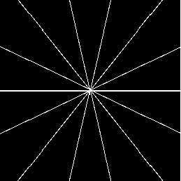
(a) $\mathcal{M}_{1},S_{r}=3\%$

(b) $\mathcal{M}_{2},S_{r}=6\%$

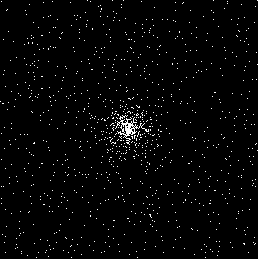
(c) $\mathcal{M}_{3},S_{r}=2\%$

Figure 1: Sampling Masks

In this section we report the results of several tests run on simulated under-sampled data obtained by synthetic (phantoms) and full resolution MRI images. The under-sampled data $z$ are obtained as $z=\Phi u$ where $u$ is the full resolution image and $\Phi$ is the under-sampling Fourier matrix, obtained as in (5). The under-sampling masks, analyzed in the next paragraphs are: radial mask ($\mathcal{M}_{1}$), parallel mask ($\mathcal{M}_{2}$) and random mask ($\mathcal{M}_{3}$). In figure 1 we represent an example of each mask with low sampling rate $S_{r}$, measured by the percentage ratio between the number of non-zero pixels $N_{\mathcal{M}}$ and the total number of pixels $N^{2}$:

$$S_{r}=\frac{N_{\mathcal{M}}}{N^{2}}\%.$$ (48)

The quality of the reconstructed image $u$ is evaluated by means of the Peak Signal to Noise Ratio (PSNR)

$$PSNR=20\log_{10}\frac{\max(x)}{rmse},\ \ \ \ rmse=\sqrt{\frac{\sum_{i}\sum_{j}(u_{i,j}-x_{i,j})^{2}}{N^{2}}}$$

where $rmse$ represents the root mean squared error and $x$ is the true image. All the algorithms are implemented in Matlab R16 on a PC equipped with Intel 7 processor and 8GB Ram.

In the first two paragraphs (4.1, 4.2) we test FNCR on synthetic data in order to asses its performance in case of critical under-sampling both on noiseless and noisy data. Finally in paragraph 4.3 data from real MRI images are used to compare FNCR to one of the most efficient reconstruction algorithms [13].

4.1 Algorithm performance on noiseless data

In this paragraph we test the performance of FNCR algorithm in reconstructing good quality images from highly under-sampled data. We focus on two synthetic images: the Shepp-Logan phantom (T1) (figure 2(a)), widely used in algorithm testing, and the Forbild phantom (T2) [21] (figure 2(b)), well known as a very difficult test problem.

In this first set of tests we stop the outer iterations of the FNCR algorithm 3.3 as soon as $PSNR\geq 100$ or $\bar{n}>5000$. The value $PSNR=100$ indicates an extremely good quality reconstruction since our test images are scaled in the interval $[0,1]$, therefore $rmse\simeq 10^{-5}$.

In table 3 we report the results obtained for the different test images and masks. In column $1$ the type of mask is reported, column $2$ contains the sampling rate $S_{r}$ of each test (in brackets the number of rays or lines for masks $\mathcal{M}_{1}$ or $\mathcal{M}_{2}$, respectively), finally for each test image, T1 (columns $3-4$) and T2 (columns $5-6$) we report the PSNR of the starting image $\Phi^{t}z$ ($PSNR_{0}$) and the value $\bar{n}$, computed as in Algorithm 3.3 and measuring the computational cost. When the algorithm stops because the maximum number of iterations has been reached ($\bar{n}=5000$), we report between brackets the last PSNR obtained.

		T1		T2
	$S_{r}$	$PSNR_{0}$	$\bar{n}(PSNR)$	$PSNR_{0}$	$\bar{n}(PSNR)$
$\mathcal{M}_{1}$	$3\%(7)$	15.7	4500	15.02	5001 (28.4)
	$5.7\%(12)$	16.8	339	16.93	378
	$10.7\%(18)$	18.8	190	18.69	233
	$25\%(60)$	22.6	96	21.8	131
$\mathcal{M}_{2}$	$6.3\%(16)$	14.6	1309	12.8	5001(29.95)
	$12.5\%(32)$	16.2	778	13.9	386 (30.9)
	$25\%(64)$		209	19.1	121 18.5
$\mathcal{M}_{3}$	$2\%$	16.2	419	15.98	5001 (31.7)
	$12\%$	17.1	106	16.7	128
	$25\%$	18.3	82	18.6	114

Table 3: FNCR results with masks $\mathcal{M}_{1}-\mathcal{M}_{3}$ on noiseless data. $S_{r}$ is the Sampling Ratio as in (48), $PSNR_{0}$ refers to the PSNR of the starting image $\Phi^{t}z$, $\bar{n}$ is the total number of Forward-Backward iterations in Algorithm 3.3. In brackets the number of rays or lines for masks $\mathcal{M}_{1}$ or $\mathcal{M}_{2}$, respectively.

We observe that T1 always reaches a PSNR value greater than 100 even with very severe under-samplings. The T2 confirms to be a very difficult test problem especially in case of $\mathcal{M}_{2}$ under-sampling mask.

We conclude our analysis of the FNCR performance with a few observations about the input parameters of Algorithm 3.3. In table 4 we report the values of $r_{0}$, $\gamma$ and $\beta$ used in the present reconstructions and notice that the parameters $r_{0}$ and $\gamma$ depend on the mask. We observe that the algorithm uses the same parameters for $\mathcal{M}_{2}$ and $\mathcal{M}_{3}$, while it requires smaller values of $r_{0}$ and $\gamma$ for $\mathcal{M}_{1}$. The parameter $\beta$ is mainly affected by the data noise and in the present experiments $\beta=1$ gives always the best results.

	$r_{0}$	$\gamma$	$\beta$
$\mathcal{M}_{1}$	$10^{-4}$	$5\cdot 10^{-2}$	1
$\mathcal{M}_{2}$,$\mathcal{M}_{3}$	$5\cdot 10^{-2}$	$5\cdot 10^{-1}$	1

Table 4: FCNR input parameters for noiseless data.

Concerning the value of the tolerance parameter $\tau$ in the stopping criterium (47) we analyze here how it affects the efficiency of the proposed matrix splitting method (46) both in terms of accuracy and computational cost.

As representative examples we report the results obtained with $\tau\in[10^{-4},10^{-1}]$ in the case of radial sampling $\mathcal{M}_{1}$ with $S_{r}=3\%$ for both T1 and T2. As shown in figure 3, where different lines represent the $PSNR$ obtained as a function of the iterations with different values of $\tau$, we have two possible situations: in the T1 test (figure 3(a)) the PSNR value 100 is always obtained, while in the second case (figure 3(b)) the $PSNR$ never gets the expected value 100. Regarding the computational cost, we plot in figure 4 the number $tot\_in$ of the total iterations required in step $\ell$ (as computed in Algorithm 3.3) as a function of the iterations, using different lines for different values of $\tau$. We note that the computational cost is minimum when $\tau\geq 10^{-3}$ and greatly increases when $\tau\leq 10^{-4}$, hence a small tolerance parameter $\tau$ is never convenient since it increases the computational cost and it does not help to improve the final PSNR. We can conclude that very few iterations of the iterative method are sufficient to solve the linear system (39) with good accuracy.

Therefore, all the experiments reported in the present section are obtained using $\tau=0.1$. In this case only $4$ inner iterations $\bar{m}$ are required by Algorithm 3.2 for each FB step and the total computational cost of FNCR is $\bar{n}\cdot 4$.

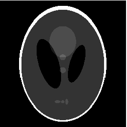
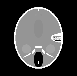
(a)                                             (b)

Figure 2: Test Images. (a) Shepp Logan (T1), (b) Forbild (T2)

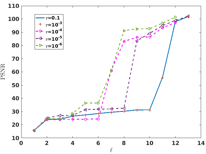
(a) T1 test

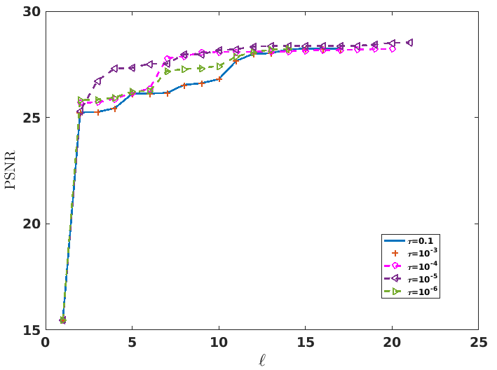
(b) T2 test

Figure 3: PSNR vs. the iterations $\ell$, for different tolerance parameters $\tau$ in (47). Mask $\mathcal{M}_{1}$ with $S_{r}=3\%$. Tolerances $\tau=0.1$ and $\tau=10^{-3}$ are represented by blue line and red crosses; $\tau=10^{-4}$ is represented by magenta line and circles; $\tau=10^{-5}$ is represented by cyan line and left triangles finally $\tau=10^{-6}$ is represented by green line and right triangles.

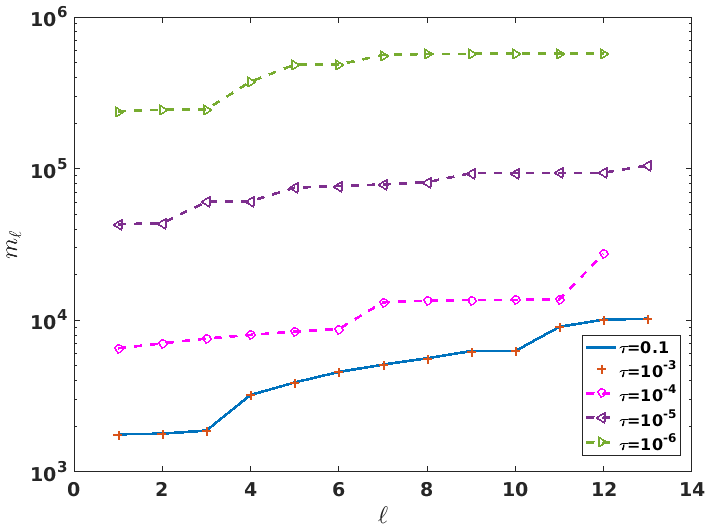
(a) T1 test

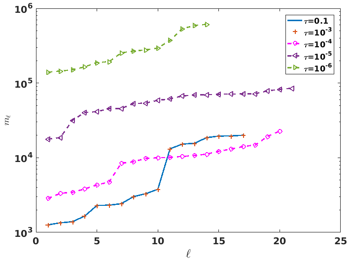
(b) T2 test

Figure 4: $Tot\_in$ vs. the iterations $\ell$ for different tolerance parameters $\tau$ in (47). Mask $\mathcal{M}_{1}$ with $S_{r}=2\%$. Left: Shepp-Logan test. Tolerances $\tau=0.1$ and $\tau=10^{-3}$ are represented by blue line and red crosses; $\tau=10^{-4}$ is represented by magenta line and circles; $\tau=10^{-5}$ is represented by cyan line and left triangles finally $\tau=10^{-6}$ is represented by green line and right triangles.

4.2 Noise Sensitivity

In this paragraph, we explore the noise sensitivity of the proposed FNCR method by reconstructing the test images from noisy data with different under-sampling masks. The simulated noisy data $z^{\delta}$ are obtained by adding to the undersampled data $z$ normally distributed noise of two different levels $\delta=10^{-3},10^{-2}$:

$$z^{\delta}=z+\delta\|z\|v,\ \ \ \|v\|=1$$ (49)

where $v$ is a unit norm random vector obtained by the Matlab function randn. Regarding the FNCR parameters, we used the same values as in table 4 for $\mathcal{M}_{2}$ and $\mathcal{M}_{3}$ masks, whereas we used $r_{0}=10^{-2}$ and $\gamma=0.2$ for mask $\mathcal{M}_{1}$.

In table 5 we report the best results obtained by the FNCR algorithm in terms of $PSNR$ and number $\bar{n}$ of FB iterations.

Compared to the results obtained in the noiseless case (table 3), we observe that the $PSNR$ value is smaller but still acceptable ($>30$) in most cases for the noise level $\delta=10^{-3}$. For the higher noise level $\delta=10^{-2}$, the reconstructions are more difficult, especially for low sampling rates.

Concerning the radial sampling $\mathcal{M}_{1}$ and random sampling $\mathcal{M}_{3}$, the Forbild data (T2) are badly reconstructed for $S_{r}=4.3\%$ and $S_{r}=3\%$ respectively, where the Shepp-Logan data (T1) always reach $PSNR>30$. The most critical problem is the parallel under-sampling $\mathcal{M}_{2}$ with $\delta=10^{-2}$, in this case both T1 and T2 reach $PSNR>30$ only with $S_{r}\geq 25\%$. Moreover $\mathcal{M}_{2}$ with $\delta=10^{-3}$ is critical only for Forbild data (T2) with $S_{r}=6.3\%$. Finally, for each test (T1, T2) we report in figures 5 and 6 the images whose $PSNR$ values are typed in bold in table 5. We can appreciate the overall good quality of the reconstructions from noisy data.

			T1	T2
	$\delta$	$S_{r}$	$PSNR(\bar{n})$	$PSNR(\bar{n})$
$\mathcal{M}_{1}$	$10^{-3}$	$4.3\%$	59.61 (130)	30.85 (192)
		$7.7\%$	66.23 (72)	60.78 (66 )
		$10.7\%$	68.61 (57)	62.84(807)
	$10^{-2}$	$4.3\%$	39.5 (461)	24.56 (44)
		$7.7\%$	43.69 (35)	36.82 (117)
		$10.7\%$	46.36 (27)	41.06 (405)
$\mathcal{M}_{2}$	$10^{-3}$	$6.3\%$	34.08 (1210)	20.2 (768)
		$12.5\%$	55.95 (590)	30.81 (228)
		$25\%$	69.75 (68)	34.76 (67)
	$10^{-2}$	$6.3\%$	22.5 (962)	17.93 (578)
		$12.5\%$	26.87 (60)	22.54 (63)
		$25\%$	52.7 (52)	33.04 (44)
$\mathcal{M}_{3}$	$10^{-3}$	$3\%$	64.4 (462)	53.5(485)
		$12\%$	64.81 (242)	62.45 (63)
		$25\%$	71.45 (58)	65.27 (241)
	$10^{-2}$	$3\%$	33.54 (134)	23.55 (418)
		$12\%$	43.29 (37)	42.99 (45)
		$25\%$	50.57 (42)	45.72 (225)

Table 5: FNCR results with masks $\mathcal{M}_{1}-\mathcal{M}_{3}$ on noisy data. $\delta$ is the noise level (49), $S_{r}$ is the Sampling Ratio (48) and $\bar{n}$ is the total number of Forward-Backward iterations in Algorithm 3.3.

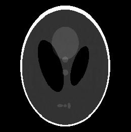
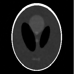
(a)                                             (b)

Figure 5: Images reconstructed from T1 noisy data. (a) $PSNR=52.7$ (b) $PSNR=43.29$.

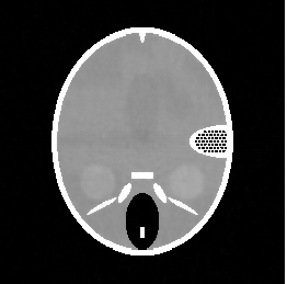
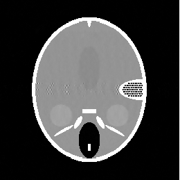
(a)                                             (b)

Figure 6: Images reconstructed from T2 noisy data. (a) $PSNR=41.06$ (b)$PSNR=22.54$.

4.3 Comparison with other methods

In this paragraph we compare the FNCR algorithm with the very efficient algorithm IL${}_{1}-\ell_{q}$ recently proposed in the literature [13], where the authors minimize a class of concave sparse metrics $\ell_{q}(q=0.5)$ in a general DCA-based CS framework. Both synthetic and real MRI data are tested. In [13] the authors test their method on T1 image with radial mask $\mathcal{M}_{1}$ and they show that a perfect ($PSNR\geq 100$) can be obtained with 7 rays. Performing the same test FNCR also reaches $PSNR\geq 100$ in comparable times.

Then we applied both methods to the T2 test image both methods with mask $\mathcal{M}_{1}$ and we obtained perfect reconstructions with $10$ sampled projections, while decreasing the projections to $8$ IL${}_{1}-\ell_{q}$ obtains $PSNR=28.7$ and FNCR reaches $PSNR=98.1$(see Figure 7).

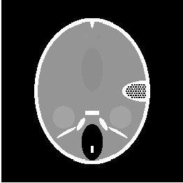
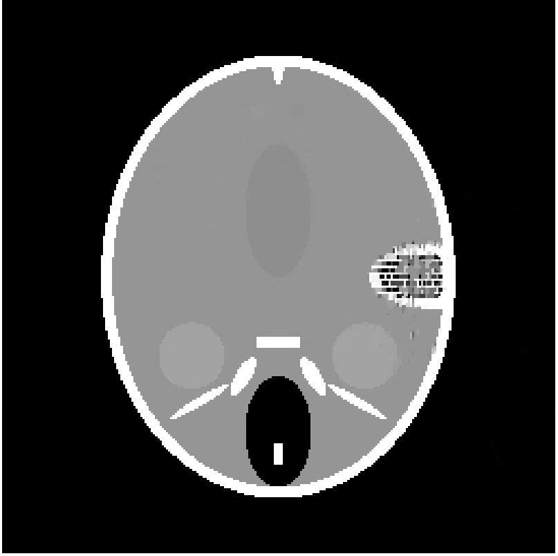
(a)                                             (b)

Figure 7: T2 test image, radial sampling mask ($\mathcal{M}_{1}$) $8$ lines ($S_{r}=3.98$): (a) FNCR reconstruction, (b) IL${}_{1}-\ell_{q}$ reconstruction.

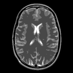
Figure 8: MRI $256\times 256$ brain image.

Concerning the real MRI data we compare IL${}_{1}-\ell_{q}$ and FNCR algorithms in the reconstructions of the $256\times 256$ brain image (T3 test), represented in figure 8. We report in table 6 the results obtained by reconstructing the noiseless data undersampled by $\mathcal{M}_{1}$, $\mathcal{M}_{2}$, $\mathcal{M}_{3}$ masks.

From the table, we see that FNCR always outperforms IL${}_{1}-\ell_{q}$.

In figure 10 we show the FCNR and IL${}_{1}-\ell_{q}$ reconstructions in case of mask $\mathcal{M}_{3}$ and $Sr=8\%$.

Finally in figure 9 we plot the reconstructed rows corresponding to the largest error (200-th row) for the true image and the FNCR reconstruction (Figure 9(a)) and for the true image and IL${}_{1}-\ell_{q}$ reconstruction (Figure 9(b)). We observe that FNCR better fits the corresponding row of the original image.

		IL${}_{1}-\ell_{q}$		FNCR
	$S_{r}$	PSNR	Time	PSNR	Time
$\mathcal{M}_{1}$	$10.60\%$	100.29	13.46s	100.3	13.88
	$9.02\%$	27.68	28.70	32.24	27.67s
$\mathcal{M}_{2}$	$25\%$	50.41	6.15s	60.54	47.98s
	$12.5\%$	33.87	19.32s	34.74	87.84s
$\mathcal{M}_{3}$	$10\%$	100.01	4.22s	100.1	6.26s
	$8\%$	30.22	28.45s	100.2	37.34s
	$5\%$	25.46	28.06	27.46	6.77s

Table 6: Comparison between FNCR and IL${}_{1}-\ell_{q}$ reconstructions on T3 test using $\mathcal{M}_{1}$, $\mathcal{M}_{2}$, $\mathcal{M}_{3}$ masks.

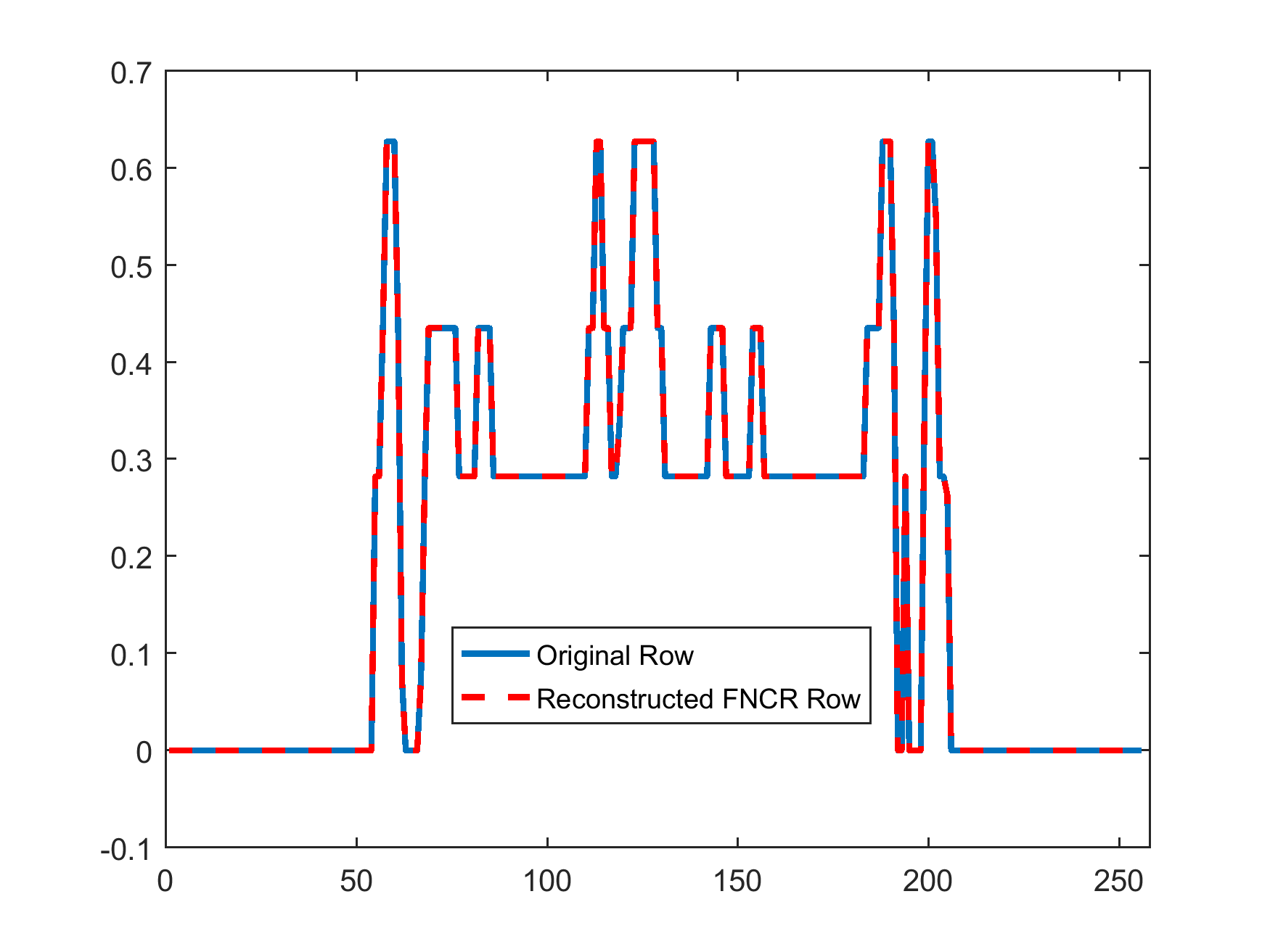
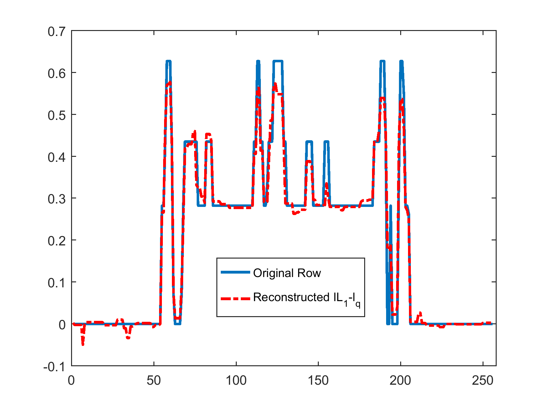
(a)                                             (b)

Figure 9: Row 200 of T3 image. Reconstructions obtained with $\mathcal{M}_{2}$ $Sr=8\%$and Mask undersampling $\mathcal{M}_{3}$, $Sr=8\%$. (a) original and FNCR reconstruction, (b) original and IL${}_{1}-\ell_{q}$ reconstruction.

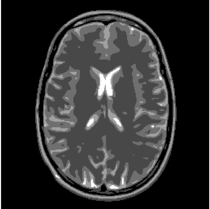
(a)                                             (b)

Figure 10: T3 image reconstructions with $\mathcal{M}_{3}$ and $S_{r}=8\%$: (a) FNCR reconstruction, (b) IL${}_{1}-\ell_{q}$ reconstruction.

We can finally conclude that FNCR is more competitive than IL${}_{1}-\ell_{q}$ in reconstructing difficult test images from very severely undersampled data.

5 Conclusions

We presented a new algorithm, called Fast Non Convex Reweighting, to solve a non-convex minimization problem by means of iterative convex approximations. The resulting convex problem is solved by an iterative Forward-Backward (FB) algorithm, and a Weighted Split-Bregman iteration is applied in the Backward step. A new splitting scheme is proposed to improve the efficiency of the Backward steps.

A detailed analysis of the algorithm properties and convergence is carried out. The extensive experiments on image reconstruction from undersampled MRI data show that FNCR gives very good results in terms both of quality and computational complexity and it is more competitive in reconstructing test problems with real images from very severely under-sampled data.

Appendix A Convergence

Aim of this subsection is to prove that the iterates $\bar{u}^{(h)}$, computed by Algorithm 3.1, converge to a local minimum of problem (12).
To this purpose we consider both the nonconvex functional

$${\cal P}(\lambda_{h},F_{\mu_{\ell}}(Du),u)=\left\{\lambda_{h}F_{\mu_{\ell}}(Du)+\frac{1}{2}||\Phi u-z||_{2}^{2}\right\}$$ (50)

and its convex majorizer

$${\cal P}(\lambda_{h},{\cal F}_{h,\mu_{\ell}}(Du),u)=\left\{\lambda_{h}{\cal F}_{h,\mu_{\ell}}(Du)+\frac{1}{2}||\Phi u-z||_{2}^{2}\right\}.$$ (51)

The approximate solution, computed by Algorithm 3.1 in (19), can be written as:

$$\bar{u}^{(h)}=\arg\min_{u}{\cal P}(\lambda_{h-1},{\cal F}_{h-1,\mu_{\ell}}(Du),u).$$ (52)

Since ${\cal F}_{h-1,\mu_{\ell}}(Du)$ is a local convex approximation of the nonconvex function $F_{\mu_{\ell}}(Du)$ at each step $h$ of the iterative reweighting method, then from (13) we have:

$${\cal F}_{h-1,\mu_{\ell}}(D\bar{u}^{(h-1)})=F_{\mu_{\ell}}(D\bar{u}^{(h-1)})\quad\mbox{ and}\quad\quad{\cal F}_{h-1,\mu_{\ell}}(Du)\geq F_{\mu_{\ell}}(Du)\ \ \ u\neq\bar{u}^{(h-1)}.$$ (53)

The following result proves the descent property of the iterative reweighting method.

Proposition A.1.

Let $\lambda_{h-1}$ and $\lambda_{h}$ be two values of the penalization parameter such that $\lambda_{h-1}>\lambda_{h}$ and let $\bar{u}^{(h)}$ and $\bar{u}^{(h+1)}$ be the corresponding minimizers given by (52), then the nonconvex functional ${\cal P}(\lambda,F_{\mu_{\ell}}(Du),u)$ satisfies the following inequality:

$${\cal P}(\lambda_{h-1},F_{\mu_{\ell}}(D\bar{u}^{(h)}),\bar{u}^{(h)})>{\cal P}(\lambda_{h},F_{\mu_{\ell}}(D\bar{u}^{(h+1)}),\bar{u}^{(h+1)})$$

Proof: Using relation (50) and the first part of property (53), rewritten for $h$ we have:

$${\cal P}(\lambda_{h-1},F_{\mu_{\ell}}(D\bar{u}^{(h)}),\bar{u}^{(h)}) =\frac{1}{2}||\Phi\bar{u}^{(h)}-z||_{2}^{2}+\lambda_{h-1}F_{\mu_{\ell}}(D\bar{u}^{(h)})$$

$$=\frac{1}{2}||\Phi\bar{u}^{(h)}-z||_{2}^{2}+\lambda_{h-1}{\cal F}_{h,{\mu_{\ell}}}(D\bar{u}^{(h)})$$

From the assumption $\lambda_{h-1}>\lambda_{h}$ it follows that:

$$\frac{1}{2}||\Phi\bar{u}^{(h)}-z||_{2}^{2}+\lambda_{h-1}{\cal F}_{h,\mu_{\ell}}(D\bar{u}^{(h)})>\frac{1}{2}||\Phi\bar{u}^{(h)}-z||_{2}^{2}+\lambda_{h}{\cal F}_{h,\mu_{\ell}}(D\bar{u}^{(h)})$$

Using (52):

$$\frac{1}{2}||\Phi\bar{u}^{(h)}-z||_{2}^{2}+\lambda_{h}{\cal F}_{h,\mu_{\ell}}(D\bar{u}^{(h)})\geq\frac{1}{2}||\Phi\bar{u}^{(h+1)}-z||_{2}^{2}+\lambda_{h}{\cal F}_{h,\mu_{\ell}}(D\bar{u}^{(h+1)})$$

Applying the second part of property (53) to the case $Du\equiv D\bar{u}^{(h+1)}$:

$$\frac{1}{2}||\Phi\bar{u}^{(h+1)}-z||_{2}^{2}+\lambda_{h}{\cal F}_{h,\mu_{\ell}}(D\bar{u}^{(h+1)})\geq\frac{1}{2}||\Phi\bar{u}^{(h+1)}-z||_{2}^{2}+\lambda_{\ell}F_{\mu_{\ell}}(D\bar{u}^{(h+1)})$$

From definition (50):

$$\frac{1}{2}||\Phi\bar{u}^{(h+1)}-z||_{2}^{2}+\lambda_{h}F_{\mu_{\ell}}(D\bar{u}^{(h+1)})={\cal P}(\lambda_{h},F_{\mu_{\ell}}(D\bar{u}^{(h+1)}),\bar{u}^{(h+1)})$$

hence:

$${\cal P}(\lambda_{h-1},F_{\mu_{\ell}}(D\bar{u}^{(h)}),\bar{u}^{(h)})>{\cal P}(\lambda_{h},F_{\mu_{\ell}}(D\bar{u}^{(h+1)}),\bar{u}^{(h+1)})$$

This proves the result. ∎

In order to prove the convergence we need the following results.

Proposition A.2.

Let’s define the bounding set $B$ s.t. $\bar{u}^{(h)}\in B$, $\forall h\geq 0$, let’s assume that $F_{\mu_{\ell}}$ and ${\cal F}_{h,\mu_{\ell}}$ have a locally Lipschitz continuous gradient on $B$ with a common Lipschitz constant $\tilde{L}\geq 0$, let’s assume also that ${\cal P}(\lambda_{h},{\cal F}_{h,\mu_{\ell}}(Du),u)$ is strongly convex with convexity parameter $\nu>0$, then the following properties hold:

1. Descent property:

   $${\cal P}(\lambda_{h-1},F_{\mu_{\ell}}(D\bar{u}^{(h)}),\bar{u}^{(h)})>{\cal P}(\lambda_{h},F_{\mu_{\ell}}D\bar{u}^{(h+1)}),\bar{u}^{(h+1)})$$ (54)

2. There exists $C>0$ such that for all $\ell\in N$ there exists

   $$\xi_{h+1}\in\partial{\cal P}(\lambda_{h},F_{\mu_{\ell}}(D\bar{u}^{(h+1)}),\bar{u}^{(h+1)})$$

   fulfilling

   $$\|\xi_{h+1}\|_{2}\leq C\|\bar{u}^{(h+1)}-\bar{u}^{(h)}\|_{2}$$ (55)

3. For any converging subsequence $\left\{\bar{u}^{(h_{j})}\right\}_{j\in N}$ with

   $$\bar{\bar{u}}\equiv\lim_{j\rightarrow\infty}\bar{u}^{(h_{j})},$$

   and $\left\{\lambda_{h_{j}}\right\}$ with $\bar{\bar{\lambda}}=\lim_{j\rightarrow\infty}\lambda_{h_{j}}$, we have

   $${\cal P}(\lambda_{h_{j}},F_{\mu_{\ell}}(D\bar{u}^{(h_{j})}),\bar{u}^{(h_{j})})\rightarrow{\cal P}(\bar{\bar{\lambda}},F_{\mu_{\ell}}(D\bar{\bar{u}}),\bar{\bar{u}})\quad j\rightarrow\infty.$$ (56)

Proof: Using proposition A.1 we can prove the descent property (54). Relations (55) and (56) can be easily proved as in [22], proposition 5. ∎

Proposition A.3.

The sequence $\bar{u}^{(h)}$ generated by Algorithm (3.1) converges to a local minimum of problem (12) for each $\ell$.

Proof: We observe that the objective function

$$\left\{\lambda_{h}F_{\mu_{\ell}}(Du)+\frac{1}{2}\|\Phi u-z\|_{2}^{2}\right\},\ \ \lambda>0.$$

satisfies the Kurdika-Lojasiewicz property [23]. In fact it is an analytic function, because the function $\psi$ in (14) is evaluated in nonnegative arguments, therefore we can restrict the domain of $\psi$ on $R^{+}\cup\{0\}$.
Finally the convergence immediately follows from [22], where the authors prove that the Iterative Reweighted Algorithm converges, provided that the relations (54), (55), (56) hold and the objective function satisfies the Kurdika-Lojasiewicz property. ∎

Appendix B Proof of theorem 3.1

In order to prove theorem 3.1 we first prove the following lemma.

Lemma B.1.

Let $M=E+F$ where $E$ is the Identity matrix and $F=\beta\theta\Delta^{w}$ with $\theta,\beta>0$. If $0<{\theta}<\frac{1}{\beta\|\Delta^{w}\|_{\infty}}$ then $M$ is a symmetric positive definite matrix.

Proof.

By definition of $\Delta^{w}$ in (36), it easily follows that $M=(I+\beta\theta\Delta^{w})$ is a real symmetric matrix. Moreover in the finite discrete setting the $k$-th component of the product $\Delta^{\omega}u$ is:

$$\left(\Delta^{\omega}u\right)_{k}=-(\alpha_{k}^{2}+\alpha_{k+1}^{2}+\eta_{k}^{2}+\eta_{k+N}^{2})u_{k}+\alpha_{k+1}^{2}u_{k+1}+\\ \alpha_{k}^{2}u_{k-1}+\eta_{k+N}^{2}u_{k+N}+\eta_{k}^{2}u_{k-N}$$ (57)

where

$$\alpha_{k}=\psi^{\prime}_{\mu_{\ell}}(|u_{x}^{(h)}|_{i,j})\ \ \eta_{k}=\psi^{\prime}_{\mu_{\ell}}(|u_{y}^{(h)}|_{i,j})\ \ k=(i-1)N+j$$ (58)

Hence on each row there are at most five non zero elements given by:

$$M_{k,k}$$= ,

= ,

= ,

= ,

=

(59)

In order to guarantee that the matrix $B$ is positive definite, it is sufficient to determine $\theta$ such that $M$ is strictly diagonally dominant, namely

$$\left|1-\beta\theta(\alpha_{k}^{2}+\alpha_{k+1}^{2}+\eta_{k}^{2}+\eta_{k+N}^{2})\right|>\beta\theta(\alpha_{k}^{2}+\alpha_{k+1}^{2}+\beta_{k}^{2}+\eta_{k+N}^{2})\\ \quad\forall\,\,k=1,...,N^{2}$$

$$\frac{1}{\beta\theta}>2(\alpha_{k}^{2}+\alpha_{k+1}^{2}+\eta_{k}^{2}+\eta_{k+N}^{2})\quad\forall\,\,k=1,...,N^{2}$$

It easily follows that this relation is satisfied for

$$\beta\theta<\max_{k=1,..N^{2}}\left(2(\alpha_{k}^{2}+\alpha_{k+1}^{2}+\eta_{k}^{2}+\eta_{k+N}^{2})\right)$$

namely,

$$0<{\theta}<\frac{1}{\beta\|\Delta^{w}\|_{\infty}}$$ (60)

∎

Proof of theorem 3.1

Proof.

Using the Householder-Johns theorem [24, 25] $\rho(E^{-1}F)<1$ iff $A$ is symmetric positive definite (SPD) and $E^{*}+F$ is symmetric and positive definite, where $E^{*}$ is the conjugate transpose of $E$. The matrix $A$ is SPD since it is symmetric and strictly diagonal dominant. From Lemma B.1, we have $E^{*}+F=M$ and therefore the condition on $\theta$ guarantees that $E^{*}+F$ is symmetric and positive definite. ∎

References

- [1] E. Candes, J. Romberg, and T. Tao. Robust uncertainty principles: exact signal reconstruction from highly incomplete frequency information. IEEE Tr. Inf. theory, 52:489–509, 2006.
- [2] D. Donoho. Compressed sensing. IEEE Trans. inf. theory, 52(4):1289–1306, 2006.
- [3] U. Gamper, P. Boesiger, and S. Kozerke. Compressed sensing in dynamic MRI. Magn. Res. imag., 59:365–373, 2008.
- [4] A. Majumdar. Improved dynamic mri reconstruction by exploiting sparsity and rank-deficiency. Magnetic Resonance Imaging, 31(5):789 – 795, 2013.
- [5] G. Landi, E.L. Piccolomini, and F. Zama. A total variation-based reconstruction method for dynamic mri. Computational and Mathematical Methods in Medicine, 9(1):69–80, 2008.
- [6] M. Lustig, D. Donoho, and J. Pauly. Sparse mri: the application of compressed sensing for rapid mr imaging. Magn. Res. in Medic., 58:1182–1198, 2007.
- [7] S. Wang et al. Iterative feature refinement for accurate undersampled mr image reconstruction. Phys. Med. Biol., 61(9):3291–3316, 2016.
- [8] Rick Chartrand. Fast algorithms for nonconvex compressive sensing: Mri reconstruction from very few data. In IEEE International Symposium on Biomedical Imaging (ISBI), 2009.
- [9] J. Trzasko and A. Manduca. Highly undersampled magnetic resonance image reconstruction via homotopic -minimization. IEEE Transactions on Medical Imaging, 28(1):106–121, Jan 2009.
- [10] Xiaoqun Zhang, Martin Burger, Xavier Bresson, and Stanley Osher. Bregmanized nonlocal regularization for deconvolution and sparse reconstruction. SIAM J. IMAGING SCIENCES, 3:253–276, 2010.
- [11] R. Chartrand. Exact reconstruction of sparse signals via nonconvex minimization. IEEE Sig. proc. Lett., 14:707–710, 2007.
- [12] Penghang Yin, Yifei Lou, Qi He, and Jack Xin. Minimization of for compressed sensing. SIAM Journal on Scientific Computing, 37(1):A536–A563, 2015.
- [13] Penghang Yin and Jack Xin. Iterative minimization for non-convex compressed sensing. 2016. UCLA CAM Report 16-20.
- [14] D. Lazzaro, E. Loli Piccolomini, and F. Zama. Efficient compressed sensing based mri reconstruction using nonconvex total variation penalties. J. of Physics: Conf. series, 756:012004, 2016.
- [15] Laura B. Montefusco, Damiana Lazzaro, and Serena Papi. A fast algorithm for nonconvex approaches to sparse recovery problems. Signal Processing, 93(9):2636 – 2647, 2013.
- [16] L. B. Montefusco and D. Lazzaro. An iterative based image restoration algorithm with an adaptive parameter estimation. IEEE Transactions on Imagel Processing, 21(4):1676–1686, 2012.
- [17] D. Lazzaro. Fast weighted tv denoising via an edge driven metric. Appl. Math. Comp., 297:61–73, 2017.
- [18] E.J. Candes and M.B. Wakin. Enhancing sparsity by reweighted l1. Journal of Fourier Analysis and Applications, 14:877–905, 2008.
- [19] A. Beck and M. Tebulle. Fast gradient-based algorithms for constrained total variation image denoising and deblurring problems. IEEE Tran. on Imag. Proc., 18(11):2419–2434, 2009.
- [20] P. L. Combettes and V. R. Wajs. Signal recovery by proximal forward-backward splitting. Multiscale Modeling & Simulation, 4(4):1168–1200, 2005.
- [21] Z. Yu, F. Noo, F. Dennerlein, A. Wunderlich, G. Lauritsch, and J. Hornegger. Simulation tools for two-dimensional experiments in x-ray computed tomography using the FORBILD head phantom. Phys. Med. Biol., 57(13), 2012.
- [22] P. Ochs, A. Dosovitskiy, T. Brox, and T. Pock. On iteratively reweighted algorithms for nonsmooth nonconvex optimization in computer vision. SIAM Journal on Imaging Sciences, 8(1):331–372, 2015.
- [23] H. Attouch, J. Bolte, and B. F. Svaiter. Convergence of descent methods for semi-algebraic and tame problems: proximal algorithms, forward–backward splitting, and regularized gauss–seidel methods. Math. Program Ser. A, 137:91–129, 2013.
- [24] J. Ortega. Matrix Theory: a Second Course. pub-PLENUM, 1987.
- [25] Zhi-Hao Cao. A note on p-regular splitting of hermitian matrix. SIAM Journal on Matrix Analysis and Applications, 21(4):1392–1393, 2000.