Dynamic of plumes and scaling during the melting of a Phase Change Material heated from below

Abstract

We identify and describe the main dynamic regimes occurring during the melting of the PCM n-octadecane in horizontal layers of several sizes heated from below. This configuration allows to cover a wide range of effective Rayleigh numbers on the liquid PCM phase, up to $\sim 10^{9}$, without changing any external parameter control. We identify four different regimes as time evolves: (i) the conductive regime, (ii) linear regime, (iii) coarsening regime and (iv) turbulent regime. The first two regimes appear at all domain sizes. However the third and fourth regime require a minimum advance of the solid/liquid interface to develop, and we observe them only for large enough domains. The transition to turbulence takes places after a secondary instability that forces the coarsening of the thermal plumes. Each one of the melting regimes creates a distinct solid/liquid front that characterizes the internal state of the melting process. We observe that most of the magnitudes of the melting process are ruled by power laws, although not all of them. Thus the number of plumes, some regimes of the Rayleigh number as a function of time, the number of plumes after the primary and secondary instability, the thermal and kinetic boundary layers follow simple power laws. In particular, we find that the Nusselt number scales with the Rayleigh number as $Nu\sim Ra^{0.29}$ in the turbulent regime, consistent with theories and experiments on Rayleigh-Bénard convection that show an exponent $2/7$.

1 Introduction

The high latent heat involved in the solid/liquid phase change allows Phase Change Materials (PCM) to store or release a significant amount of energy during melting or solidification barely changing the temperature. Many technological applications take advantage of this stability on external temperature variations and thermal storage capacity to use these materials in electronic cooling, air conditioning in buildings, waste heat recovery, to compensate the time offset between energy production and consumption in solar power plants, or combining with construction materials to increase the thermal energy storage capacity of with lighter structures [1, 2, 3, 4].

The usage of PCM for latent heat storage is attracting much interest and promotion of regulatory authorities during the last years due to environmental issues and requirements of efficiency of renewable energy sources [5, 6]. The melting temperature allows classifying the PCM in low temperature ($<200^{\circ}C$) and high temperature ($>200^{\circ}C$) categories [7]. Organic PCM such as paraffins are common among the low temperature category due to their stability in melting and freezing cycles, non-corrosive and suffering no under-cooling. An enormous amount of experimental, numerical and modeling work has been carried out to understand the heat transfer performance of these materials taking into account only conductive heat transport within the liquid phase of the PCM and including as well convective transport [8, 9, 10].

The operation cycle of PCM consist of two phases: (i) a charging phase when the PCM melts, releasing the latent heat of the solid to liquid transition and developing a solid/liquid front that moves from hotter to colder regions, (ii) a discharging phase when the PCM solidifies creating a front moving in the opposite direction. We will focus on this work in the melting phase of the cycle. When only conductive transport is involved, the symmetry of the system dictates the form of these fronts. However, when convective transport appears the coupling between hydrodynamics, temperature field, phase change and propagation of the interface results in corrugated fronts. The shape of the fronts is more readily available on experiments than velocity and temperature fields in the liquid phase of the PCM. Hence this shape can provide information on the melting state of a PCM if a relation with the front shape can be established. We will show in this work how melting regimes have distinct front shapes.

After the selection of the PCM material, the geometry of the PCM container is the most influential factor in the heat transport performance of PCM systems. Many of the studies have been concerned with the heat transfer in cylinders, cylinder shells, rectangular cavities heated from the side [11, 12, 13, 14, 15, 10, 16] or even irregular non-symmetric geometries [17, 18, 19]. However, the configuration of a PCM within a rectangular container heated from below has received comparably less attention. From a practical point of view, this configuration is important to dissipate heat from electronic devices. From a theoretical point of view, it offers the opportunity to understand the effect of the phase change on convection when comparing with well established results of the classic Rayleigh-Bénard problem on convective features, heat transport, stability and scaling [20, 21]. This problem of a PCM contained within rectangular cavities and heated from below has been studied in simulations with paraffins, ice slurries or cyclohexane, etc. [22, 23, 24, 25], and experiments with cyclohexane, n-octadecane or magma, among others [26, 27, 28].

We focus on this work at studying the dynamic of melting of the paraffin n-octadecane, wich belongs to the low temperature group of PCM. The n-octadecane is contained in squares with periodic boundary conditions in the horizontal direction of different sizes and heated from below. This configuration makes possible to explore a broad range of effective Rayleigh numbers, taking as characteristic length the gap of the melted PCM, without changing any external parameter. For the largest domains, we reach Rayleigh numbers $\sim 10^{9}$. At this high numbers, the convective features depend very meaningfully on the existence of persistent thermal plumes [29]. We study in this work how they emerge and evolve during the charging phase.

The Rayleigh-Bénard problem of a liquid layer heated from below is characterized by three physical magnitudes: the difference of temperature between the plates, the heat flux, and the type of fluid. These provide three dimensionless numbers: Rayleigh $Ra$, Nusselt $Nu$ and Prandtl $Pr$; respectively, which characterize the solutions of this problem. At the regime of high numbers, the relation between Rayleigh and Nussselt numbers $Nu\equiv Nu(Ra,Pr)$ has been thoroughly studied and found that mostly matches a power law $Nu\sim Ra^{\alpha}$ [30]. The exponent $\alpha$ generally is within a range between $1/4$ and $1/3$ and the numerical results show a dependence of the exponent with $Ra$ [31, 32, 33, 34] as well as experiments [35, 36, 37, 38].

A theory by Malkus [39] based on arguments of marginal stability of the thermal boundary layer predicts $Nu\sim Ra^{1/3}$ and a large number of experiments agree with this scaling [40]. However, when heat transfer and turbulence decouple from the thermal and viscosity transport coefficients there is as well a theoretical prediction for an asymptotic regime following $Nu\sim Pr^{1/2}\,Ra^{1/2}$ [41, 42]. Interestingly, the limit of infinite Prandtl number predicts as well $Nu\sim Ra^{1/3}$ for the regime of asymptotically high Rayleigh numbers [32, 43]. Nevertheless, it must be noticed that not all the experimental studies have agreed with the theoretical scalings. Thus, models based on a mixing layer [35], turbulent boundary layer [44] and extensions to low Prandtl fluids [45] predict an exponent $2/7$.

We aim in this work at studying the convective motion in the presence of a solid/liquid phase change. The presence of phase change introduces an additional number related to the source of latent heat, the Stefan number, that complicates the problem. In spite of that, we find that the averaged value of the numeric exponent $0.29$ is consistent with a group of experiment results [35, 46, 45, 47, 48] on moderately high Rayleigh numbers $Ra<10^{10}$, and theoretical models predicting $2/7$.

The article is organized as follows. Section 2 describes the governing equations of the mathematical model we use to simulate the behavior of a PCM in the presence of conductive and convective transport. The numeric procedure and code to solve the previous equations are explained in Section 3. We present in Section 4 the results of our simulations, where we explain the observed melting regimes, transitions between them and establish relations between dynamic quantities characteristics of the melting process. Finally, we discuss in Section 5 our most important findings and provide a brief outline of our work.

2 Model of Phase Change Materials

We consider a PCM whose solid phase is modeled with a heat equation to account for conductive transport of the heat, and the liquid phase is modeled with the Navier-Stokes equations for momentum coupled to the energy equation to include in this phase the heat transport by convection. The Navier-Stokes equations are modified with a Darcy term to model a diffuse interface between the solid and liquid phases, and the energy equation includes a source term to account for the release of latent heat during melting. A comprehensive derivation and explanation of the model used in this work can be found in references [49] and [50]. We now describe the main features of the model equations and their coupling.

2.1 Momentum equations

We consider the flow as laminar, incompressible, and neglect the viscous dissipation due to the small domains involved. The difference in density between liquid and solid phases of n-octadecane is about $5\%$ and is neglected in the model for simplicity.

The governing equation expressing the balance of momentum has the vectorial form

$$\rho\left[\frac{\partial\vec{u}}{\partial t}+\left(\vec{u}\cdot\nabla\right)\vec{u}\right]=-\nabla p+\mu\nabla^{2}\vec{u}-\rho\,g\left[1-\alpha(T-T_{ref})\right]\vec{e_{y}}-\frac{C(1-f_{l})^{2}}{\delta+f_{l}^{3}}\vec{u},$$ (1)

where $\nabla=(\partial_{x},\partial_{y})$ and $\partial_{t}$ are the spatial and temporal operators respectively. $T$ is a temperature averaged in a control volume, which can contain pure solid (volume liquid fraction $f_{l}=0$), liquid (volume liquid fraction $f_{l}=1$) or a mixture of both phases ($0<f_{l}<1$) in local thermal equilibrium; $\vec{u}=(u_{x},u_{y})$ is the fluid velocity, being $u_{x}$ and $u_{y}$ the horizontal and vertical components; $\rho$ is the PCM density whose variation between liquid and solid phases is neglected; $\mu$ is the dynamic viscosity, $p$ is the pressure, $g$ the magnitude of gravity acceleration, $\vec{e_{y}}$ a unit vector pointing in the vertical direction upwards, $T_{ref}$ is a reference temperature where physical properties are given and $\alpha$ the thermal expansion coefficient. The bulk physical properties are supposed to be constant within the range of temperatures studied, expect the density in the buoyancy term that follows a linear dependence with the temperature according to the Boussinesq approximation.

The last term in the momentum equation provides an empirical proportionality relationship, due to Darcy, between the pressure gradient in a porous medium and the fluid velocity within it. The functional form corresponds to the Carman-Kozeny equation and is a convenient way to damp the velocity flow within the mushy region and suppress it at the solid phase. We set in this term the Darcy coefficient $C=1.6\cdot 10^{6}kg\,m^{-3}\,s$, in compliance with previous works ([51, 19]), and $\delta<<1$ a tiny constant to avoid division by zero without physical meaning. When the cell is completely liquid ($f_{l}=1$) the Darcy term is null, like in a single phase fluid, when it is completely solid ($f_{l}=0$) the Darcy term becomes dominant, and the velocity of the liquid becomes null. For intermediate values of $f_{l}$ ($0<f_{l}<1$), the PCM is in the mushy zone. Through this formulation, the Darcy term allows to use the momentum equation in the whole domain and model the phase change when fluid motion is present without the complication of tracking the solid/liquid interface ([49, 50]).

2.2 Energy equation

The thermal energy of the system comes from the contribution of the usual sensible heat, due to changes in the temperature of the solid and liquid phases of the PCM, and from the latent heat content. Assuming the same density in each phase, it can be expressed as a function of the temperature as follows

$$\left[\frac{\partial}{\partial t}+\vec{u}\cdot\nabla\right]\rho\left((1-f_{l})C_{s}+f_{l}C_{l}\right)T=\nabla\left((1-f_{l})\lambda_{s}+f_{l}\lambda_{l}\right)\nabla T-\rho\Delta h\frac{\partial f_{l}}{\partial t}$$ (2)

where $C_{s}$ ($C_{l}$) and $\lambda_{s}$ ($\lambda_{l}$) are the specific heats and conductivities of the PCM in the solid (liquid) phase averaged with the liquid fraction, and $\Delta h$ is the latent heat of the solid/liquid phase change of the PCM.

The latent heat released by a control volume during the solid to liquid phase change depends on the melted PCM given by liquid fraction as $\Delta H=f_{l}\rho\Delta h$ being $H$ the enthalpy. As a consequence, the coupling between the energy and momentum equations is given through the liquid fraction field $f_{l}$, which in turn depends on the temperature, the master variable of the phase change process. We model the liquid fraction in the mushy zone using a linear relationship between the solidus and liquidus temperatures

$$f_{l}=\Delta H/(\rho\Delta h)=\left\{\begin{array}[]{l}0,\quad T\leq T_{s}\\ 1,\quad T\geq T_{l}\\ (T-T_{s})/(T_{l}-T_{s}),\quad T_{s}<T<T_{l}\end{array}\right.$$ (6)

$\Delta H$ ranges from $0$ (PCM completely solid) to $\rho\Delta h$ (PCM completely melted). Liquid and solid phases coexist for intermediate values. Notice that the small value $(T_{l}-T_{s})/(T_{h}-T_{m})\sim 0.026$ used in this work creates a mushy region with a width of only some hundredths of micrometers, leading to neglectable latent heat advection. A thorough discussion of this can be in [50] and shown numerically in [52].

	$\rho(\frac{kg}{m^{3}})$	$C_{pcm}(\frac{m^{2}}{s^{2}K})$	$\lambda_{pcm}(\frac{kgm}{s^{3}K})$	$\mu(\frac{kg}{ms})$	$\alpha(\frac{1}{K})$	$T(K)$	$\Delta h(\frac{m^{2}}{s^{2}})$
liquid phase	776	2196	0.13	0.0036	$9.1\cdot 10^{-4}$	299.65	$243.5\cdot 10^{3}$
solid phase		1934	0.358			298.25

Table 1: Physical properties of n-octadecane [19]. Liquid and solid values are given when distinguised at the model equations.

2.3 Domain and boundary conditions

We solve the equations in a set of horizontal layers in the form of squares with periodic boundary conditions along the horizontal direction of sides from $L=0.005\,m$ to $L=0.2\,m$ heated from below. The bottom wall is conductive and held at constant temperature $T_{h}=353.15\,K$, greater than the melting temperature of n-octadecane ($T_{l}=298.65\,K$) which is held initially at solid state at a homogeneous temperature $T_{i}=298.15\,K$. The upper wall is supposed to be adiabatic, excluding heat exchange with the surroundings.

N-octadecane is a representative viscous paraffin with Prandtl number $Pr=60.3$ and latent heat typical of this group of materials $L=243.5\cdot 10^{3}\,J\,Kg^{-1}$. The thermo-physical properties within the liquid and solid phases used in the simulations are listed in Table 1.

2.4 Dimensionless numbers

We calculate an effective Rayleigh number in this work as $Ra=\frac{g\,\alpha\Delta T\,h^{3}}{\kappa\,\nu}$, where $\Delta T=T_{h}-T_{m}$, and $h$ is not the size of the domain but the averaged height of the melted PCM [53]. Notice that the Rayleigh number is time dependent due to the continued advance of the melting front. Since the interface is diffuse, we choose the cells with liquid fraction $f_{l}=0.5$ as the criterium for the height of the interface. This liquid fraction corresponds to the mean temperature of the phase transition $T_{m}=(T_{s}+T_{l})/2$.

The local Nusselt number is calculated as $Nu_{x}=\frac{h(x)\,\left.\partial T/\partial y\right|_{y=0}}{T_{h}-T_{m}}$. Notice that this expression is not the same as commonly used in Rayleigh-Bénard convection. Instead of using the height of the domain, we use the height of the solid/liquid interface $h(x)$ and the differences of temperature between this interface and the hot wall at the bottom. As a consequence, the Nusselt number is not $1$ when conduction prevails on the liquid phase due to the finite thickness of the interface. This definition of the local Nusselt provides a more accurate computation of the relative strength between convective and conductive flux. From now on, we will discuss our results using the averaged Nusselt number along the horizontal axis $Nu=\frac{1}{L}\int_{0}^{L}Nu_{x}\,dx.$

Finally, the Stefan number of the melting process is defined as $Ste=c_{l}\,(T_{h}-T_{l})/\Delta h$, which throws a fixed value $0.49$ in this work.

3 Numerical methods

We use the open source software under GPL license OpenFOAM [54], based on finite volumes to simulate the evolution along the time of the model discussed in the previous section. The conservation of fluxes ensured by the finite volume method makes this discretization especially advantageous when non-linear advective terms appear as in convection dominated PCM dynamics. The convective terms are discretized using a second order upwind scheme. The time integration is carried out using a second order Crank-Nicolson scheme. The solver automatically limits the time step using a maximum Courant-Friedrichs-Lewy condition. Also, we have imposed a maximum temporal step of $0.5\,s$ to ensure robustness for all the tested conditions. The source term in the energy equation requires particular attention since it couples the temperature and liquid fraction fields strongly. Following [55], it is linearized as a function depending on temperature, split in an explicit (zero order term) and implicit part (first order term), and the liquid fraction updated at every iteration. A Rhie-Chow interpolation method is used to solve the enthalpy-porosity equations to avoid checkerboard solutions. The momentum and continuity equation are solved using the PIMPLE algorithm, which ensures a right pressure-velocity coupling by combining SIMPLE and PISO algorithms [56]. The temperature equation is solved for each PIMPLE outer-iteration, securing the convergence of the velocity, pressure, and temperature fields.

Regarding the validation of the model, the proper implementation of the bulk equations has been extensively verified with numeric and experimental works to ensure the stability and accuracy of the code, with special care of the treatment of the source term of the energy equation in [57]. The implementation is very successful in modeling the strong coupling between momentum and energy equations typical of phase change problems in rectangular and geometries in the form of circular sections [19, 58, 57].

We have used a structured and uniform mesh of $400\times 400$ cells for domain size from $0.005\,m$ to $0.1\,m$. This provides a maximum grid size of $2.5\cdot 10^{-4}\,m$ for $L=0.1\,m$. For $L>0.1\,m$ we use $800\times 800$, providing a grid size of $2.5\cdot 10^{-4}\,m$ for $L=0.2\,m$. Notice how these grid resolutions resolve the Kolmogorov scale $\eta(y)=\left(\mu^{3}/\epsilon_{u}\right)^{1/4}$, where $\epsilon_{u}(y)=\frac{\mu}{L}\int_{0}^{L}{\left(\partial u^{\prime}_{i}/\partial x_{j}\right)^{2}}\,dx$ is the turbulent dissipation and $\vec{u^{\prime}}$ the fluctuation about a spatial average of the velocity on the horizontal axis [59]. Thus, for instance, for $L=0.04\,m$ we obtain from our simulations $min(\eta)=8.6\cdot 10^{-4}\,m$, and for $L=0.1\,m$ we obtain $min(\eta)=6\cdot 10^{-4}\,m$, where the function min provides the minimum value of the Kolmogorov scale from the beginning up to complete melting of the PCM.

4 Results

4.1 Regimes

We identify up to four dynamic regimes during the melting of the n-octadecane. Next, we describe them and show how they depend on the domain size.

4.1.1 Conductive regime

	a) $t=50s$	b) $t=100s$	c) $t=300s$	d) $t=440s$
Stream Function
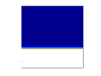
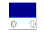
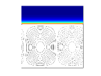
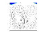
Temperature field

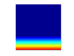
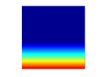
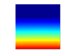
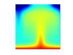
Figure 1: Snapshots at different times $t=50,100,300,440s$ for the stream function (top row) and temperature field (bottom row) for a domain of side $L=0.005\,m.$

The conductive regime starts at the beginning of melting and is governed by conductive heat transfer. The PCM is melted above the hot wall, there is not convective motion within the liquid phase, and a solid/liquid interface parallel to the hot wall develops moving upwards.

This regime is common to all domain sizes, and Fig. 1(a) illustrates this state for the smallest domain of this study $L=0.005\,m$ at $t=50\,s$. The height of the interface advances in time following a power law $h\sim t^{0.49}$ with a similar exponent for the rest of sizes $L$. The value of this exponent agrees remarkably well with that of the position of the solid/liquid interface of the analytic two-phase Stefan problem in a semi-infinite slab $\sim t^{1/2}$. In the Stefan problem, the interface is supposed to be sharp, with zero thickness. It is worth noticing that in spite of adopting a model with a diffuse interface in this work the value of the numerical exponent is very close to the Stefan problem with a sharp interface.

4.1.2 Linear regime

As time advances, a second regime arises after the destabilization of the conductive layer through a linear Rayleigh-Bénard instability and the ensuing convective motion. Indeed, for a horizontal layer of n-octadecane bounded by rigid plates, it suffices a thickness $\sim 1.5\,mm$ to destabilize the conductive state. The instability creates an array of counter-rotating convective cells and lengthening plumes.

Fig. 1 (b,c,d) show the evolution of this regime through a sequence of panels for the temperature and velocity fields for $L=0.005\,m$, and Fig. 2 for $L=0.01\,m$. The wave number of the primary instability allows a single plume fitting into the domain for $L=0.005\,m$. As time advances, the stem lengthens, and the head of the plume widens resulting in a plume with a form of mushroom. The widening and form of the head are responsible for a curved solid/liquid interface. During this process, there are two symmetric counter-rotating cells around the stem with preserved width.

	a) $t=100s$	b) $t=200s$	c) $t=300s$	d) $t=400s$
Stream Function
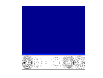
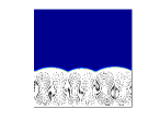
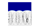
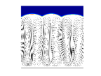
Temperature field

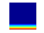
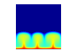
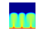
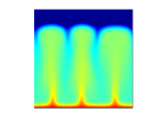
Figure 2: Snapshots at different times $t=50,100,300,400s$ for the stream function (top row) and temperature field (bottom row) for a domain of side $L=0.01\,m.$

For greater domain sizes, like $L=0.01\,m$ in Fig. 2, an array of plumes develop without interaction between them. The heads of this array of plumes generate a modulated melting front as appears in experiments of melting of n-octadecane by Gau and Viskanta (c.f. Fig 1a, 1b of Ref. [60]).

The separation between the plumes is determined by the critical wavenumber of the primary Rayleigh-Bénard instability and is conserved during this regime. As a consequence, this wavenumber determines the distance between peaks of the melting front. Given that the main features of this regime come from the linear instability mode of the conductive regime, we refer to it as the linear regime.

This second melting regime exhibits relatively low Rayleigh numbers $<O(10^{5})$. While the main dynamic features of this regime occur along the vertical direction we notice that when melting advances the stems of the plumes begin to bend, with roughly fixed stem location on the thermal boundary layer. Indeed, the thermal boundary layer extends along the hot wall with its thickness barely changing. This is opposed to plumes created by point sources of heat [29].

	a) $t=200s$	b) $t=500s$	c) $t=550s$	d) $t=570s$
Stream Function
Temperature field
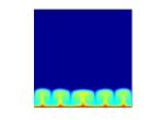
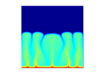
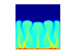
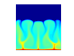
	e) $t=590s$	f) $t=600s$	c) $t=620s$	d) $t=670s$
Stream Function
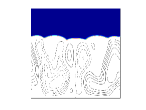
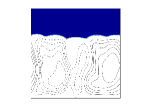
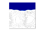
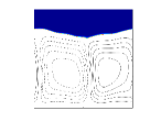
Temperature field

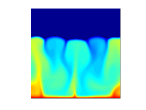
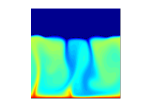
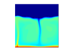
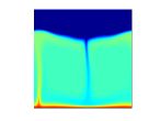
Figure 3: Sequence of snapshots for the stream function (top row) and temperature field (bottom row) at different times for a domain of side $L=0.02\,m$. The sequence shows the coarsening of five plumes in the first panel into a single plume in the last panel after suffering a secondary instability.

4.1.3 Coarsening regime

With the further advance in melting appears a regime where the convective cells of the linear regime destabilize and merge up to recover roughly an aspect ratio close to the cells at the onset of the Rayleigh-Bénard instability. Notice that this aspect ratio is the fraction of the average depth of the convective cells with respect to the domain size $L$. This merging takes places with the coarsening of the thermal plumes of the linear regime.

Figs. 3 and 4(left) show the coarsening and development of this secondary instability in time through a sequence of snapshots of the temperature and velocity fields for $L=0.02\,m$ and $L=0.04\,m$, respectively.

A closer look at the early stage of the linear regime ($t=500\,s$ in Fig. 3, or $t=400\,s$ in Fig. 4) shows that the stem of some plumes becomes very deflected in their central section. Next, the stem and cells begin to move erratically up to the coarsening of the plumes. This occurs with a central plume holding roughly a non-deflected stem, and the neighbor plumes exhibiting the largest deflections. This suggests the existence of a horizontal mode with a finite wavenumber during the coarsening of the plumes. Indeed, as observed for $L=0.04\,m$ the beginning of the secondary instability shows the stems deflecting in a periodic form along the horizontal direction.

During the coarsening, the solid/liquid front loses the periodicity characteristic of the linear regime becoming irregular in some regions. This loss of symmetry happens with a smooth increase in the amplitude of the modulations of the interface. Once the coarsening stage is completed, a new periodic solid/liquid interface is reached with lower wavenumber.

Remarkably, the completion of the coarsening phase occurs with the cells recovering an aspect ratio similar to the convective cells at the onset of the Rayleigh-Bénard instability. This is illustrated in Fig. 5, where the aspect ratio of the convective cells is plotted at the threshold of the coarsening regime (circles) and after the coarsening regime is completed (squares). The maximum aspect ratio reached by the convective cells is bounded between $4.7$ and $7.5$ for all domain sizes $L$. Although this maximum ratio does not decrease monotonously with $L$, there is an overall decreasing trend with higher $L$. After merging is completed we obtain an averaged value of the aspect ratio of $1.4$. The same average value of the aspect ratio of the convective cells at the origin of the first instability, shown as well in Fig. 5 with green diamonds. However the aspect ratio with respect to $L$ after the coarsening exhibits much larger fluctuations about the mean than after the first instability.

The evolution after the coarsening regime depends on the domain size. For large $L$, there is room for additional interplay between phase separation and convective motion before complete melting, and we generally find a transition towards a turbulent state. However, in some case such as $L=0.04\,m$ a third instability occurs developing a second coarsening (c.f. Fig. 4(right)). This creates a behavior similar to a coarsening cascade. After this second coarsening the number of cells is reduced to one to recover again an aspect ratio close to the cells of the first instability. This aspect ratio is shown in Fig. 5 as a black star.

While no systematic studies have been carried out on this state in the context of melting of PCM heated from below on the scaling of $Nu$, boundary layers or statistics of plume, we notice that using related models Prudhome [61] showed snapshots of merged convective cells in a cylinder heated from below, and Gong et al.[22] showed the merging of convective cells and plumes at different times within square geometries heated from below taking the domain size as the characteristic length for the Rayleigh number.

	First coarsening			Second coarsening
	Stream Function	Temperature field		Stream Function	Temperature field
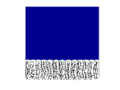
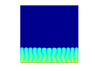
$t=400s$			$t=600s$
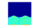
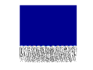
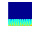
$t=420s$			$t=750s$
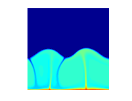
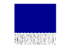
$t=440s$			$t=765s$
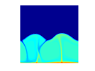
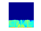
$t=460s$			$t=770s$
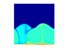
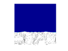
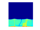
$t=480s$			$t=780s$
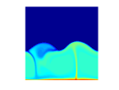
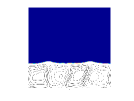
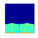
$t=500s$			$t=800s$

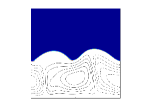
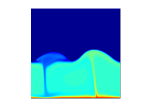
Figure 4: Stream function (left) and temperature field (right) for a domain of side $L=0.04\,m$ at different times. The sequence shows a first coarsening of the thermal plumes between $400\,s$ and $500\,s$, and a second coarsening after $600\,s$.

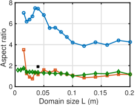
Figure 5: Aspect ratio (defined as the ratio of the average depth of the convective cells to the domain size $L$) of the convective cells before the first coarsening (blue circles) and once it is completed (red squares) versus the domain side $L$. The aspect ratio of the convective cells appearing after the first (Rayleigh-Bénard) instability is shown with green diamonds. The lonely black point corresponds to the aspect ratio after the second coarsening (third instability) of $L=0.04\,m$.

4.1.4 Turbulent regime

Finally, for large enough domains ($L>0.035\,m$ in the geometries tested) a fourth regime appears as the latest stage of melting after the coarsening regime. It is characterized by a high deformation of the thermal boundary layer on the hot wall and the emergence of new plumes no related to coarsening phenomena. Flow fields and plume dynamic are erratic in this regime. This is the regime where most of the melting occurs for the larger domains. Fig. 6 at $L=0.08\,m$ shows a sequence of snapshots of the temperature and velocity fields for this regime from $320\,s$. It can be observed how small hot plumes emerge from the hot wall and strong variations of the thickness occur on the thermal boundary layer. As we will see based on scaling arguments, this regime is similar to the classic turbulent regime observed in high Rayleigh number convection.

	a) $t=320s$	b) $t=400s$	c) $t=450s$	d) $t=500s$
Stream Function
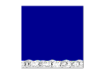
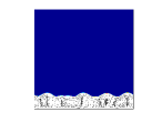
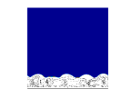
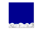
Temperature field
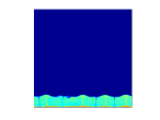
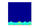
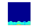
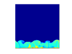
	e) $t=550s$	f) $t=600s$	c) $t=750s$	d) $t=1000s$
Stream Function
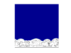
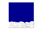
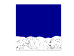
Temperature field

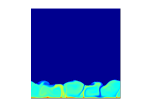
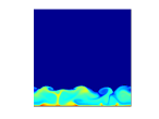
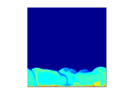
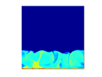
Figure 6: Snapshots of the turbulent regime at times $t=320,400,450,500,550,600,750,1000\,s$ for the stream function (top row) and temperature field (bottom row) for a domain of side $L=0.08\,m$. Strong variations in the thermal boundary layer, erratic motion and small plumes arising from the hot wall are observed.

4.2 Evolution of the Rayleigh number

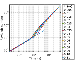
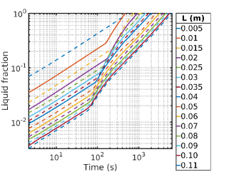
Figure 7: Rayleigh number as a function of time for all domain sizes (left). Liquid fraction as a function of time for all domain sizes considered (right)

We now characterize the regimes described previously with measures related to the Rayleigh number, the Nusselt number, the number of plumes and the thickness of the thermal and kinetic boundary layers.

Fig. 7(a) shows a log–log plot of the Rayleigh number as a function of the time for all domain sizes. Every curve stops when melting of the PCM is complete for the corresponding domain size. The curves start as straight lines in the log-log plot following a power law averaged over all the domain sizes $Ra\sim t^{1.47}$. The exponent provides an averaged front height dependence on time as $h\sim t^{0.49}$. This region is within the conductive melting regime, and this time dependence of the Rayleigh number extends up to the beginning of the linear regime. After entering into the linear regime, the simple power law of the conductive regime is lost and the melting rate is accelerated with a stronger increase of $Ra$ with time. Indeed, the linear regime with lengthening plumes barely interacting between them, exhibits the fastest advance of the solid/liquid interface during the melting of the PCM.

For domain sizes $L>0.035\,m$ the system is large enough to access the turbulent regime. Interestingly, at this regime a simpler power law behavior is recovered at the late stages of melting with averaged $Ra\sim t^{2.46}$. Fig. 7(b) shows a log-log representation of $Ra$ with respect to the liquid fraction that allows to distinguish better the different melting regimes. The growth of $Ra$ with time during the turbulent regime is lower than during the linear regime, but higher than in the conductive regime. The smallest growth rate during the conductive regime indicates how the convective motion accelerate the melting rate. The beginning of the coarsening and turbulent regime is not clearly identified from the $Ra$ curves, however we will show how measures based on the Nusselt number are more suitable to indentify these.

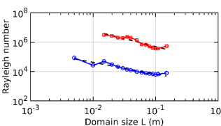
a)  b)
 
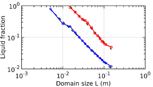
c)

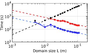
Figure 8: Left panel (a): Rayleigh number with respect to the domain size $L$ at the onset the first (blue circles) and second (red squares) instabilities. The dashed black lines correspond to power laws $Ra\sim L^{-0.85}$ and $Ra\sim L^{-0.87}$ for the first and second instability, respectively.
Right panel (b): Same thresholds represented with the overall liquid fraction, fitted with $f_{l}\sim L^{-1.31}$ and $f_{l}\sim\,L^{-1.27}$ for the first and second instability, respectively. Bottom panel (c): time of complete PCM melting as a function of the domain size (black dots). The black dashed line corresponds to a fit $t\sim L^{1.1}\,s$. The times of first and second instability are included as well as blue circles and red squares, respectively and their corresponding fits are $t\sim\,L^{-0.59}$ and $t\sim L^{-0.57}$.

The onset of the linear and coarsenining regimes is anticipated with the domain size. Each point of Fig. 8(a) corresponds to the Rayleigh number at the onset of the first (blue circles) and second (red squares) instabilities for each domain size $L$. The Rayleigh number at the onset of the the first instability follows a power law as $Ra\sim L^{-0.85}$while the onset of the coarsening regime can be fitted with $Ra\sim L^{-0.87}$, indicating a similar dependence on the domain size of both regimes. Likewise, the overall liquid fraction for the first and second instabilities follows as well a power law (c.f. Fig. 8(b)), with $f_{l}\sim L^{-1.31}$ for the first instability and $f_{l}\sim L^{-1.27}$ for the second. A representation of the time of these instabilities is additionally illustrated in Fig. 8(c), where is added the time when complete PCM melting occurs. The time for complete melting follows $t\sim L^{1.1}$, indicating a progressively longer time for $L$ respect to a linear relationship. Thus a configuration of smaller domains containing the same total volume and subjected to the same boundary conditions would melt faster than a larger domain with that PCM volume.

In short, the Rayleigh number at the conductive and tuburlent regime exhibits power laws. However, the linear regime, with a simple plume lengthening dynamics, exhibits the fastest melting rate with a more involved dependence of $Ra$ with time. Besides, the onset of the first and second instabilities, and the total melting time exhibit power laws with the domain side. The coarsening and onset of the turbulent regime are not clearly distinguished on the evolutive Rayleigh curves.

4.3 Number of plumes

The number of plumes emerging from the hot wall after the linear Rayleigh-Bénard instability depends on the domain size. This number fits a power law $N_{primary}=455.7\,L^{1.1}$ as seen in Fig. 9. Since this figure is only provided for a set of sizes, a step function (solid blue line) has been superposed to delimitate the boundaries between consecutive sizes. We have compared the quality of fits between straight lines and power laws. While for small $L$ the difference between both fits is small, it becomes meaningful for large $L$ where the power law matches better the number of plumes. Furthermore, Fig. 9 shows with squares the number of plumes after suffering the secondary instability and completed the coarsening as a function of $L$. In this case, the difference between the linear and power law fits is smaller but the residuals for the power law fit are less skewed. Thus the power law matches better the numeric data with $N_{secondary}=151.8\,L^{1.24}$. Comparing the exponents of these power laws, we obtain a weakening trend towards the formation of plumes after the secondary instability with $L$. Unfortunately we have not identified an adequate number of cases for the secondary coarsening to come to a conclusion whether this trend is obeyed for a tertiary instability.

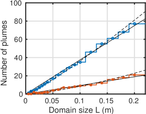
Figure 9: Number of thermal plumes after the primary (blue symbols) and secondary (red symbols) instability as a function of the size of the domain in meters $L$. The solid lines correspond to the best linear fits $N_{primary}=375\,L$ and $N_{secondary}=94.54\,L$, and the dashed lines correspond to the best power law fits $N_{primary}=455.7\,L^{1.1}$ and $N_{secondary}=151.8\,L^{1.24}$.

4.4 Evolution of the Nusselt number

We investigate the relation between the heat flux represented by the Nusselt number, which is calculated as described in Sec. 2.4, and the strength of buoyancy represented by the Rayleigh number in Fig. 10(a). Since $T_{h}$ is fixed and we have a moving solid/liquid interface, the curves $Nu$ v.s. $Ra$ are effectively $Nu$ v.s. $h^{3}$. The conductive, linear, coarsening and turbulent regimes are remarkably well distinguished in this representation of the melting dynamic. The quick destabilization of the conductive regime after the Rayleigh-Bénard instability leading to the formation of the convective cells exhibits the fastest rate of heat flux with a very strong dependency of the Nusselt number with the Rayleigh number. This destabilization was not captured clearly in the previous charts and appears in Fig. 10 as almost vertical lines with an averaged scaling of $Nu\sim Ra^{2.81}$. After the creation of the convective cells appears the linear regime following a power law with averaged smaller exponent $Nu\sim Ra^{0.29}$.

As time progresses, the plumes begin to merge entering into the coarsening regime. This regime is short lived and surfaces in Fig. 10 as a break of the previous power law with $Nu$ fluctuating for all $L$, without a clear trend. However, $Nu$ v.s. $Ra$ representation, even better $Nu$ v.s. liquid fraction of Fig. 10(b), allows for a clear separation between the linear and coarsening regime. Table 2 lists the individual values of the exponents of the linear regime as a function of size. For very small domain sizes $L<0.05\,m$ the effect of the confinement is strong and exponents are higher that once they settle to an average $Nu\sim Ra^{0.27}$ for $L>0.05\,m$, where the exponent is not strongly affected by the system size. This exponent is slighlty lower than $2/7$ reported in a broad set of literature in high Rayleigh number convection [35, 44, 45]. This is probably due to the fact that this regime is characterized by the vertical development of plumes without meaningful interaction between them or chaotic behavior.

For large domains $L>0.035\,m$ the system supports new instabilities and the development of turbulent states. Nusselt curves at the turbulent states are characterized by high fluctuations, whose amplitude tends to escalate with $Ra$. In spite of these fluctuations, these curves follow a power law $Nu\sim Ra^{0.29}$, after averaging with all the domain sizes (c.f. Table 2). This averaged exponent is slightly above than $2/7$, and get closer to this number for the largest domain sizes. Thus the turbulent state of the melted PCM exhibits a behavior for the heat flux very close to body of literature on high Rayleigh convection that reports and exponent $2/7$ in theoretical and numerical models. This is a remarkable result since the effect of heat release during melting and corrugated and moving solid/liquid interface does not affect strongly to the scalinng between bouyoancy and heat flux.

The exponent $0.9$ found in this work agrees as well with a group of experimental results on convection at high $Ra$ numbers [35, 46, 45, 47]. Interestingly, a recent experimental article by Ditze and Scharf [48] on melting of ingots of pure metals, metal alloys and ice on their own melts reports a scaling law as $Nu\sim Ra^{0.291}$. The exponent meaningfully deviates from the predictions of literature based on lateral heating as emphasized by those authors. In this work, we find a numerical value of $Nu\sim Ra^{0.90}$ in strong agreement with this experimental results, indicating the relevance of vertical gradients of temperature in this poblem.

A representation of the Nusselt number with respect to the overall liquid fraction provides a clearer separation between the different regimes (c.f. Fig. 10(b)). We identify the threshold of the first instability with circles and the threshold of the second instability with stars in Fig. 10(b). As the overall liquid fraction for the geometry of this work corresponds to a bounded dimensionless form of the average thickness $h$, Fig. 10(b) provides the dependence of the heat flux with the position of the solid/liquid interface. As a consequence $Nu$ v.s. $f_{l}$ has the same exponents as discussed above for $Nu$ v.s. $Ra$ divided by three.

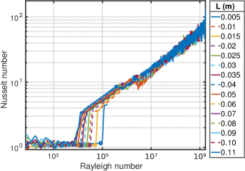
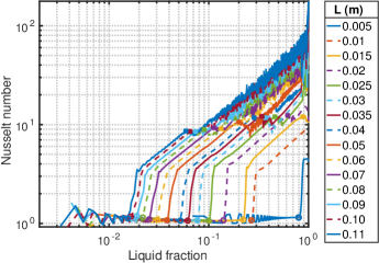
Figure 10: Nusselt number as a function of Rayleigh number for all the domain sizes considered in this work (left). Nusselt number as a function of the overall liquid fraction (right). Circles mark the threshold of the first instability and stars the second instability.

$Nu$ - $Ra$	Exponents power laws
L (m)	Linear regime	Turbulent regime
0.01	0.30	-
0.015	0.30	-
0.02	0.30	-
0.025	0.30	-
0.03	0.29	-
0.035	0.28	-
0.04	0.28	0.31
0.05	0.27	0.31
0.06	0.27	0.27
0.07	0.27	0.30
0.08	0.27	0.29
0.09	0.27	0.28
0.1	0.27	0.29
0.11	0.27	0.30
0.15	0.26	0.28
mean:	0.28	0.29

Table 2: Exponent of the power laws of the linear regime (first column) and turbulent regime (second column).

4.5 Thermal and kinetic boundary layers

The thickness of the thermal boundary layer $\delta_{T}$ can be defined in various ways. We define the thickness $\delta_{T}$ as the distance between the intersection of the tangent of the horizontally averaged temperature profile at the hot wall $\bar{T}=T_{h}+\left.d\,T/d\,y\right|_{y=0}\,y$ with the mean temperature between the hot wall and the interface $T_{m}=\frac{T_{h}+(T_{s}+T_{l})/2}{2}$. Notice how the temperature of the interface is fixed at $(T_{s}+T_{l})/2$, but its position is moving upwards, providing a $T_{m}$ that depends on increasingly distant points. As pointed out in Ref. [59] these definitions roughly correspond to the crossover point between mean dissipation and turbulent dissipation. From the definition of the averaged Nusselt number in Sec. 2.4 the thickness of the thermal boundary layer can be expressed as well as

$$\delta_{T}=\frac{h}{2\,Nu}$$ (7)

which is a more practical expression if the Nusselt curves are known.

The thickness of the thermal boundary layer $\delta_{T}$ on the hot wall as a function of $Ra$ for different $L$ is plotted in Fig. 11(a). The curves display clearly the four melting regimes: (i) the conductive regime appears as almost straight lines with positive slope in the log-log plot, (ii) the destabilization of the conductive regime produces a strong decrease of $\delta_{T}$ due to the quick enhancement of the heat flux at the bottom, (iii) the linear regime with its characteristic high heat flux exhibits the lowest values for $\delta_{T}$ once convection sets in, (iv) the turbulence shows very large fluctuations of $\delta_{T}$ with increasing amplitude when $Ra$ growths.

Interestingly, on the contrary to the problem turbulent Rayleigh-Bénard convection, where the liquid domain is fixed, the value of $\delta_{T}$ for the melted PCM increases with $Ra$ instead of decreasing [30]. Thus, for instance, we obtain $\delta_{T}\sim Ra^{0.05}$ for $L=0.1\,m$. However, we can compare with the classic Rayleigh-Bénard convection representing $\delta_{T}$ normalized with the average depth of the melted PCM, i.e. $\delta_{T}/h$ v.s. $Ra$, as shown in Fig. 11(b). Now we obtain decreasing curves with $Ra$, which follow power laws at the turbulent regime. For instance, $\delta_{T}/h\sim Ra^{-0.29}$ for $L=0.10\,m$. This value is above the Prandtl-Blassius theoretical prediction of $-0.25$. However, it agrees with values of numerical simulations of $-0.29$ for $Pr=0.7$ in a cylindrical cell with aspect ratios $1$ within a lower range de $Ra$ used in this work [62], and for with $-0.31$ obtained for an aspect ratio $1/2$ with a wider range of $Ra$ [63]. There are as well experimental works in water that report an exponent $-0.33$ [64], above as well of Prandtl-Blassius theory.

We follow [59] to define the thickness of the kinetic boundary layer $\delta_{u}$ as the distance from the hot wall to the intercept of $\overline{u}=\left.\frac{d\,\overline{u}}{d\,y}\right|_{y=0}\,y$ and $\overline{u}=max(\overline{u})$, where $\overline{u}$ is the spatial average along the horizontal axis of the module of the velocity. We observe in Fig. 4.5(a) how $\delta_{u}$ and its fluctuations increase with $Ra$; similarly to $\delta_{T}$ in the turbulent regime. However, $\delta_{u}/h$ v.s $Ra$ decreases, following a power law in the turbulent regime, for example $\delta_{u}/h\sim Ra^{-0.16}$ for $L=0.1\,m$. This scaling does not agree with the prediction of an exponent $-0.25$ from the Prandtl-Blasius theory, or with numerical and experimental results in very low Prandtl fluids that exhibit exponents close to Prandtl-Blasius [65, 66]. However, we find good agreement between our results in some experiments for liquids in cylindrical and cubic geometries covering a wide range of Prandtl numbers, reporting an exponent about $-0.16$ for the kinematic boundary layer at the bottom plate [67, 68, 69]. Similarly to the excellent agreement for $\delta_{T}/h$, Verzicco et al. [62] obtain an exponent $-0.18$ for the kinematic boundary layer in simulations with $Pr=0.7$.

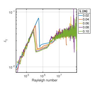
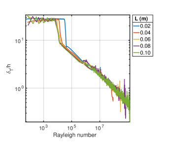
Figure 11: Left: Thickness of the thermal boundary layer $\delta_{T}$ as a function of the Rayleigh number in log-log scale. Right: Thickness of the thermal boundary layer $\delta_{T}$ scaled by the average depth of the melted PCM $h$ as a function of the Rayleigh number in log-log scale.