On the Phase Connectedness of the Volume-Constrained Area Minimizing Partitioning Problem

Abstract.

We study the stability of partitions in convex domains involving simultaneous coexistence of three phases, viz. triple junctions. We present a careful derivation of the formula for the second variation of area, written in a suitable form with particular attention to boundary and spine terms, and prove, in contrast to the two phase case, the existence of stable partitions involving a disconnected phase.

1. Introduction

The phase partitioning problem involves the splitting of a domain $\Omega\subset\mathbb{R}^{n}$ into a prescribed number of subsets, the phases, with the measure of each phase fixed, and minimality of their perimeter in the interior of $\Omega$. Investigation of interfaces and related phenomena started in the 19th century when Plateau[1] observed that soap films and bubble clusters consisted of (a) smooth surfaces, (b) curves (liquid lines) along which triples of surfaces met at equal angles, and (c) isolated points where four such triple junctions met at equal angles. Early studies of the mathematical problem of partitioning include Nitsche’s paper[2, 3], and Almgren’s Memoir[4]. White[5] proved existence and discussed regularity of equilibrium immiscible fluid configurations using Flemming’s flat chains[6]. Taylor[7, 8] characterized the minimal cones in $\mathbb{R}^{3}$. The regularity of the liquid line was established by Kinderlehrer, Nirenberg and Spruck[9].

The structure of the singular set of hypersurfaces and their clusters was studied by using mean curvature flow methods[10]. A hypersurface evolves by mean curvature flow when the velocity is given by the mean curvature vector. Volume preserving mean curvature flows were used for the investigation of the dynamics of phase partitioning problems with a volume constraint[11, 12]. These methods apply to two-phase problems. For the three-phase partitions with prescribed boundaries and triple junction topologies, the required constraints render the formulation and the handling of the problem prohibitively complex. Note that a pure mean curvature motion with nontrivial velocity is not possible near the line where the three surfaces of a triple junction intersect (the spine), see Section 5, text preceding equation (5.1). We found the direct variational methods used in this work, which allow tangential variations besides the usual normal ones, more convenient and suitable for the investigation of the stability of multiphase problems involving multijunctions.

The problem of the phase connectedness was addressed by Sternberg and Zumbrun (SZ)[13], for the particular case of two-phase partitioning. They proved that stable two phase partitions in strictly convex domains are necessarily connected. In the present paper we consider the three-phase partitioning of a domain (open and connected subset) $\Omega\subset\mathbb{R}^{3}$ (or $\mathbb{R}^{2}$) with boundary $\Sigma=\partial\Omega$, in which three phases coexist by the formation of triple junctions. $\Sigma$ is assumed to be a $C^{r}$-hypersurface of $\mathbb{R}^{3}$. Occasionally we present definitions, formulas and propositions more generally in $\mathbb{R}^{n}$, but our main results concern $\mathbb{R}^{3}$ and $\mathbb{R}^{2}$.

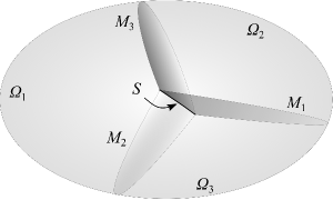
Figure 1.1. Single triple-junction partitioning. $\Omega_{i}$ is the space occupied by phase $i$ and $M_{i}$ is the interface between phases $k$, $l$ with $k\neq i$ and $l\neq i$. $S$ is the spine of the triple junction.

The problem can be mathematically formulated as follows. Let $\Omega\subset\mathbb{R}^{3}$ (or $\mathbb{R}^{2}$) be a domain with boundary $\Sigma=\partial\Omega$ as stated. In the volume constrained 3-phase partitioning problem (refer to Figure 1.1) we seek a division of $\Omega$ into three subsets (the phases) $\Omega_{1}$, $\Omega_{2}$, $\Omega_{3}$, each having prescribed volume $\left|\Omega_{i}\right|=V_{i}$, and boundaries $M_{i}$ in $\Omega$ (the interfaces), which form a triple junction $T=(M_{i})_{i=1}^{3}$, such that the total interface is a (local or global) minimizer of the area functional. The interfaces $M_{i}$ are assumed to be $C^{2}$-hypersurfaces with boundary. In a general setting, the interfaces $M_{1},\cdots,M_{m}$ form more than one triple junction (see Figure 1.2). The area, or more generally, the surface energy functional of the partitioning is given by

(1.1) $$A(T)=\sum_{i=1}^{m}\gamma_{i}A(M_{i})$$

where $\gamma_{i}>0$ is the surface energy density (surface tension) associated with $M_{i}$. In this notation, interfaces, phases and subsets are identified by successive indexing. Other indexing schemes are possible. The notation[5] $M_{ij}$ for the interfaces, where $i$, $j$ are phases in contact, was not found convenient for our calculations. More convenient notations are introduced in the sequel; refer to Example 6 for a brief comparison of indexing schemes. A minimal partitioning is a critical point of the functional (1.1),

$$\delta A(T):=\left.\frac{d}{dt}A(T^{t})\right|_{t=0}=0,$$

where $T^{t}$ is any admissible variation of the partition (for a precise formulation of this, see Definition 2). The second variation of the surface energy functional $A$ is defined by

$$\delta^{2}A(T):=\left.\frac{d^{2}}{dt^{2}}A(T^{t})\right|_{t=0}$$

A stable partition is a minimal partition with $\delta^{2}A(T)>0$ for all nontrivial admissible variations. A partition is disconnected if at least one phase $\Omega_{i}$ is a disconnected subset (see Figure 1.2).

Our main result is Theorem 31 which establishes the existence of stable partitions with a disconnected phase in convex domains of $\mathbb{R}^{2}$ by a configuration of two triple junctions (see Figure 7.1):

Theorem (Existence of stable partitions with a disconnected phase in $\mathbb{R}^{2}$).

Let $\Omega$ be a convex domain in $\mathbb{R}^{2}$, and $T=(M_{1},\cdots,M_{5})$ a minimal disconnected three-phase partitioning of $\Omega$ by a system of two $C^{2}$ triple junctions as in Figure 7.1, with volume constraints. Furthermore, for $\Omega$ and the partitioning system $T$ we make the following assumptions:

(H1) The boundary $\Sigma=\partial\Omega$ is $C^{2}$ in a neighborhood of $\Sigma\cap\overline{T}$ and it is flat at $\overline{T}\cap\Sigma$. In particular this means $\sigma=0$ at all points of $\overline{T}\cap\Sigma$.

(H2) $M_{1}$ is flat, i.e. $\kappa_{1}=0$, and the length of $M_{1}$ is $L$.

(H3) All other leaves have the same curvature $\kappa\neq 0$ and the same length $|M_{i}|=l$, $i=2,\cdots,5$.

(H4) $\alpha<0$ in the orientation of Figure 7.1.

Then there is a $L_{0}>0$, possibly depending on $l$ and $\kappa$, such that for $L\leqslant L_{0}$ the disconnected triple junction partitioning $T$ is stable.

This is in contrast to the 2-phase partitioning, indicating that the instability of disconnected partitions is specific to the 2-phase partitioning. Unstable triple junction configurations of the same topology in convex domains exist, as it is shown in Section 5. Figure 1.2 shows the geometric characteristics of stable (type II) and unstable (type I) configurations. The quantity $\alpha$ appears in the formula of the second variation of area for a triple junction system (see equations 4.48). We established Theorem 31 by proving that the second variation of the area of the double triple junction system (which is by hypothesis minimal, i.e. a critical point of the area functional) is positive for all nontrivial admissible variations. The fundamentals of the method are briefly presented in Section 6 (see also [14]).

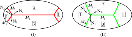
Figure 1.2. Disconnected triple junction configurations in 2-dimensional space. Boxed numbers indicate phases. Phase 1 is disconnected, while phases 2, 3 are connected in both cases. $M_{1},M_{2},M_{3}$ are the interfaces associated with the left triple junction. $N_{1},N_{2},N_{3}$ are the unit normal fields of the respective interfaces. In the shown orientation, configuration (I) has $\alpha=\frac{\sqrt{3}}{4}\left(\kappa_{2}-\kappa_{3}\right)>0$, while configuration (II) has $\alpha<0$. $\kappa_{2}$, $\kappa_{3}$ are the signed curvatures of the respective interfaces, defined by $\kappa_{i}=\left<\frac{dT_{i}}{ds},N_{i}\right>$ for each interface, $T_{i}$ being the unit tangent field of $M_{i}$, which is considered parametrized by arc length $s$.

The basis of our analysis is a formula for the second variation of area for minimal triple junction partitions with volume constraints in $\mathbb{R}^{3}$ (Theorem 12):

Theorem (2nd variation of area for minimal triple junctions with volume constraints in $\mathbb{R}^{3}$).

Let $\Omega$ be a domain in $\mathbb{R}^{3}$, $T=(T_{j})_{j=1}^{r}$, $T_{j}=(M_{pj})_{p=1}^{3}$, a minimal three-phase partition of $\Omega$ by a set of $r$ $C^{2}$ triple junctions with volume constraints, and $w$ an admissible variation satisfying (4.1) and the volume constraints. On each leaf $M_{pj}$ we have the splitting $w=u_{pj}+v_{pj}$, $u_{pj}\in TM_{pj}$, $v_{pj}\in NM_{pj}$, and we set $f_{pj}=w\cdot N_{pj}=v_{pj}\cdot N_{pj}$, $N_{pj}$ being the unit normal field of $M_{pj}$. Then the following formula holds for the second variation of the area functional,

$$\begin{gathered}\delta^{2}A^{\star}(T)=\sum_{p,j}\gamma_{pj}\int_{M_{pj}}\left(|\mathrm{grad}_{M_{pj}}f_{pj}|^{2}-|B_{M_{pj}}|^{2}f_{pj}^{2}\right)\\ -\sum_{j=1}^{r}\sum_{p=1}^{3}\gamma_{pj}\int_{\partial M_{pj}\cap\varSigma}f_{pj}^{2}II_{\varSigma}(N_{pj},N_{pj})\\ +\sum_{j=1}^{r}\sum_{p=1}^{3}\gamma_{pj}\int_{S_{j}}f_{pj}h_{pj}II_{M_{pj}}(\nu_{pj},\nu_{pj})\end{gathered}$$

where $S_{j}$ is the spine of $T_{j}$ and $\nu_{pj}\in TM_{pj}$ is the unit normal field of $\partial M_{pj}\cap S_{j}$.

As an application of this theorem, we prove in Section 5 the stability of the previously mentioned class of triple junction partitions.

In order to obtain Theorem 12, which holds in dimension three, we first need to extend the second variation formula (2.6) in the following Proposition (Proposition 9, Section 4), which works in all dimensions. The developed formulas apply to constant mean curvature manifolds allowing for tangential variations:

Proposition (2nd variation of area for constant mean curvature manifolds in $\mathbb{R}^{3}$).

Let $M$ be $C^{2}$-hypersurface of $\mathbb{R}^{n}$ with boundary. We assume that $M$ has constant mean curvature $\kappa$ and $w$ is a variation compactly supported in $M$ and whose support is contained in a chart of $M$. Further let $N$ be the unit normal field of $M$ in a chart containing the support of $w$, $\nu$ the unit outward normal of $\partial M$ which is tangent to $M$, $u=w^{\top}$, $v=w^{\bot}$, and $f=w\cdot N$. Then the second variation of the area of $M$ is given by

$$\delta^{2}A(M)= \int_{M}\left(|\mathrm{grad}_{M}f|^{2}-|B_{M}|^{2}f^{2}\right)+$$

$$\int_{M}\kappa\left[II_{M}(u,u)-2f\mathrm{div}_{M}u+\kappa f^{2}-a\cdot N\right]+$$

$$\int_{\partial M}\left[(u\cdot\nu)\mathrm{div}_{M}u-\left\langle\nabla_{u}u,\nu\right\rangle+2fII_{M}(u,\nu)+a\cdot\nu\right]$$

and for variations satisfying (4.1)

$$\delta^{2}A(M)= \int_{M}\left(|\mathrm{grad}_{M}\,f\,|^{2}-|B_{M}|^{2}f^{2}\right)+$$

$$\int_{M}\kappa\left[II_{M}(u,u)-2f\mathrm{div}_{M}u+\kappa f^{2}-a\cdot N\right]+$$

$$\int_{\partial M}\left[(u\cdot\nu)\mathrm{div}_{M}u+fII_{M}(u,\nu)+f\left\langle D_{N}w,\nu\right\rangle\right]$$

where

$$|B_{M}|^{2}=g^{ik}g^{jl}B_{ij}B_{kl}=B_{j}^{i}B_{i}^{j},\quad B_{ij}=II_{M}(E_{i},E_{j}),$$

and $\left(E_{i}(p)\right)_{i=1}^{n-1}$ is a local basis of $T_{p}M$.

The precise formulation of the variational problems considered in this paper, along with notation and well-known facts used, is given in Section 2. For the reader’s convenience, in Section 3 we briefly formulate facts related to the first variation of area in a form suitable for triple junction partitions.

2. Notation and Preliminaries

Throughout this paper we use manifolds with boundary (see [15] p. 478 for a definition).

Definition 1.

Let $\Omega$ be a domain of $\mathbb{R}^{3}$. By a $C^{r}$ triple junction in $\Omega$ (see Figure 1.1) we mean a collection of three 2-dimensional $C^{r}$ submanifolds of $\mathbb{R}^{3}$ with boundary, $(M_{i})_{i=1}^{3}$, having the same boundary in $\Omega$

$$\partial M_{i}\cap\Omega=S,\quad i=1,2,3$$

which is called the spine of the triple junction. We will refer to the manifolds $M_{i}$ as the leaves of the triple junction. Triple junctions in $\mathbb{R}^{2}$ are defined analogously.

Definition 2.

Let $M$ be a $n$-dimensional $C^{1}$ submanifold of $\mathbb{R}^{m}$ with boundary, $V$ an open subset of $\mathbb{R}^{m}$ such that $V\cap M\neq\emptyset$. A variation of $M$ is a collection of diffeomorphisms $(\xi^{t})_{t\in I}$, $I=\,]-\delta,\delta[$, $\delta>0$, $\xi^{t}:V\to V$ such that[16]

(i) The function $\xi(t,x)=\xi^{t}(x)$ is $C^{2}$

(ii) $\xi^{0}=id_{V}$

(iii) $\xi^{t}|_{V\setminus K}=id_{V\setminus K}$ for some compact set $K\subset V$. $\square$

In place of the $\xi^{t}$ we often consider their extension by identity to all of $\mathbb{R}^{m}$. With each variation we associate the first and second variation fields

$$w(x)=\xi_{t}(0,x),\quad a(x)=\xi_{tt}(0,x)$$

also known as velocity and acceleration fields[17], $\xi_{t}$, $\xi_{tt}$ denoting first and second partial derivatives in $t$. By the support of a variation we mean the support of $w$. We set $M^{t}:=\xi^{t}(M)$ for the variation of $M$.

This definition extends readily to triple junctions, which, as individual geometric objects, are not submanifolds of $\mathbb{R}^{m}$. Letting $T=(M_{i})_{i=1}^{3}$ be a triple junction, and $(\xi^{t})_{t\in I}$ a variation, the triple junctions

$$T^{t}=(\xi^{t}(M_{i}))_{i=1}^{3},\;t\in I$$

are a variation of $T$. The 1-dimensional submanifolds

$$S^{t}=\xi^{t}(S),\;t\in I$$

are a variation of the spine of $T$.

Let $M$ be a submanifold of $\mathbb{R}^{m}$. For a vector field $X$ of $\mathbb{R}^{m}$ defined on a domain $V$ of $\mathbb{R}^{m}$ we define its tangent and normal parts $X^{\top}(p)\in T_{p}M$ and $X^{\bot}(p)\in N_{p}M$, $p\in M\cap V$. $TM$ and $NM$ are the tangent and normal bundles of $M$ respectively. The notation $X\in TM$ is an abbreviation for $X(p)\in T_{p}M$ for $p$ in an open subset of $M$. Given any two vector fields $X$, $Y$ on $V$, $D_{Y}X$ denotes the directional derivative of $X$ in direction $Y$ in $\mathbb{R}^{m}$. When $u,v\in TM$,

$$\nabla_{v}u=(D_{v}u)^{\top}\in TM$$

is the covariant derivative of $u$ in direction $v$. The covariant derivative $\nabla u$ of $u$ is a $(1,1)$-tensor field defined by

$$\nabla u(\omega,v)=\omega(\nabla_{v}u),\quad v\in TM,\>\omega\in T^{\star}M,$$

where $T_{p}^{\star}M$ is the dual space of $T_{p}M$. The components of the covariant derivative $\nabla u$ are defined by

$$u_{\,|j}^{i}=\nabla u(E^{i},E_{j})=dq^{i}\left(\nabla_{E_{j}}u\right).$$

$E_{i}(p)$ is a basis of $T_{p}M$ and $E^{j}(p)\equiv dq^{j}(p)$ is the corresponding dual basis of $T_{p}^{\star}M$.

The normal part of the directional derivative $B(u,v)=(D_{v}u)^{\bot}\in NM$ defines the 2nd fundamental form tensor. The mean curvature vector is given by the trace of this tensor

(2.1) $$H(p)=\sum_{i}B_{p}(E_{i},E_{i})$$

in an orthonormal basis $(E_{i})$ of $T_{p}M$. If $M$ is a hypersurface, the scalar mean curvature is defined by

(2.2) $$\kappa=H\cdot N$$

where $N$ is a unit normal field of $M$. Similarly, when $M$ is a hypersurface of $\mathbb{R}^{m}$, we define the scalar version of the 2nd fundamental form:

(2.3) $$II_{M}(u,v)=B(u,v)\cdot N$$

The Weingarten mapping of a hypersurface $M$ of $\mathbb{R}^{n+1}$ is defined fiberwise by

$$W(p):T_{p}M\to T_{p}M,\;u\mapsto D_{u}N\quad(p\in M)$$

When index notation is used, summation over pairs of identical indices (which for tensor expressions must be pairs of contravariant-convariant indices) is assumed throughout.

The gradient of a function $f:U\to\mathbb{R}$ defined in an open neighborhood $U$ of $M$, is given by

$$\mathrm{grad}_{M}f=g^{ij}\frac{\partial f}{\partial q^{j}}E_{i}$$

in a coordinate system $q^{1},\cdots,q^{n}$. In this definition $g^{ij}$ are the contravariant components of the metric tensor $g_{ij}=E_{i}\cdot E_{j}$. The divergence of a tangent vector field $v$ of $M$ defined in $U$ is the trace of its covariant derivative, i.e.

$$\mathrm{div}v=\mathrm{tr}\nabla u=\nabla u(E_{i},E^{i})=u_{\,|i}^{i}$$

For a general vector field $w$ which is not tangent to $M$ the divergence is defined by

$$\mathrm{div}_{M}w=\left\langle D_{E_{i}}w,E^{i}\right\rangle=g^{ij}\left\langle D_{E_{i}}w,E_{j}\right\rangle$$

The notation $\left\langle\cdot,\cdot\right\rangle$ is alternately used to denote scalar product in lengthier expressions.

For the first variation of the area of a manifold with boundary, the following proposition holds.

Proposition 3.

Let $M$ be a $n$-dimensional $C^{1}$-submanifold of $\mathbb{R}^{m}$ with boundary, and $\xi^{t}$ a variation as in Definition 2, which is compactly supported in $M$. We assume that the support of $\xi^{t}$ is contained in a chart of $M$. Then the first variation of the area functional $A$ is given by

(2.4) $$\delta A(M)=\left.\frac{d}{dt}A(M^{t})\right|_{t=0}=\int_{M}\mathrm{div}{}_{M}wdS$$

If $M$ is additionally a $C^{2}$-hypersurface with boundary,

(2.5) $$\delta A(M)=-\int_{M}H\cdot wdS+\int_{\partial M}w\cdot\nu ds$$

where $\nu$ is the unit outward pointing normal vector field of $\partial M$ which is tangent to $M$, and $H$ is the mean curvature vector.

For the proof see [17, 18]. For brevity we will omit the integration symbols $dS$, $ds$.

Our formulas for the second variation of the area of triple junctions derive from the following well-known result.

Proposition 4.

Let $M$ be a $n$-dimensional $C^{2}$-submanifold of $\mathbb{R}^{m}$ with boundary, and $\xi^{t}$ a variation of $M$ compactly supported in $M$, and the support of $\xi^{t}$ is contained in a chart of $M$. Then the second variation of the area functional is given by

(2.6) $$\delta^{2}A(M) =\int_{M}\left(\mathrm{div}_{M}a+(\mathrm{div}_{M}w)^{2}+g^{ij}\left\langle(D_{E_{i}}w)^{\bot},(D_{E_{j}}w)^{\bot}\right\rangle\right.$$

$$\left.-g^{ik}g^{jl}\left\langle(D_{E_{i}}w)^{\top},E_{j}\right\rangle\left\langle(D_{E_{l}}w)^{\top},E_{k}\right\rangle\right).$$

$(E_{i})_{i=1}^{n}$ are the basis vector fields in a chart containing the support of the variation.

For the proof see [17].

The above formulas for the first variation of area extend readily to triple junctions:

(2.7) $$\delta A(T)=\left.\frac{d}{dt}A(T^{t})\right|_{t=0}=\sum_{i=1}^{3}\gamma_{i}\int_{M_{i}}\mathrm{div}{}_{M_{i}}w$$

(2.8) $$\delta A(T)=-\sum_{i=1}^{3}\gamma_{i}\int_{M_{i}}H\cdot w+\int_{S}w\cdot\sum_{i=1}^{3}\gamma_{i}\nu_{i}+\sum_{i=1}^{3}\gamma_{i}\int_{\partial M_{i}\cap\Sigma}w\cdot\nu_{i}$$

The extension of formula (2.6) for the second variation of area to triple junctions is not as straight-forward. This task is undertaken in Section 4 after proper modifications of (2.6).

3. First Variation-Young’s Equality

We treat the constraints of triple junction partitions by using Lagrange multipliers. In the simplest case of a connected partitioning, in which one triple junction is present, we consider the following modified area functional

(3.1) $$A^{\star}(T)=\sum_{i=1}^{3}\gamma_{i}A(M_{i})-\sum_{j=1}^{2}\lambda_{j}(|\Omega_{j}|-V_{j})$$

where $|\Omega_{j}|$ is the Lebesque measure of $\Omega_{j}$, and $V_{j}$ is the prescribed value for the volume of $\Omega_{j}$. The introduction of Lagrange multipliers is a matter of convenience, and one could proceed without them by properly restricting admissible variations to those preserving the volumes of the $\Omega_{j}$ (see [13, 14]). In taking the variations of (3.1) we can drop the constants $V_{i}$ altogether.

The leaves of a minimal triple junction with volume constraint are at angles $\vartheta_{i}$ according to Young’s law. We formulate this well-known fact in the simple case of a single triple junction and then extend it to a more general setting.

Proposition 5.

Let $T=(M_{i})_{i=1}^{3}$ be a $C^{2}$ triple junction partition of $\Omega\subset\mathbb{R}^{3}$ into the subdomains $\Omega_{j}$ ($j=1,2,3$). If $T$ is minimal, then Young’s equality

(3.2) $$\frac{\sin\vartheta_{1}}{\gamma_{1}}=\frac{\sin\vartheta_{2}}{\gamma_{2}}=\frac{\sin\vartheta_{3}}{\gamma_{3}}$$

holds on the spine $S$ of $T$. Furthermore, the leaves have constant (scalar) mean curvature satisfying the relation

(3.3) $$\gamma_{1}\kappa_{1}+\gamma_{2}\kappa_{2}+\gamma_{3}\kappa_{3}=0$$

where $\kappa_{i}=H_{i}\cdot N_{i}$ is the mean curvature of $M_{i}$.

Proof.

Let $(\xi^{t})_{t\in I}$ be any variation with first variation field $w$. By (3.1) we obtain

$$\delta A^{\star}(T)=\delta A(T)-\sum_{i=1}^{2}\lambda_{i}\left.\frac{d}{dt}|\Omega_{i}^{t}|\right|_{t=0}$$

where $\Omega_{i}^{t}=\xi^{t}(\Omega_{i})$. Using (2.8) and

(3.4) $$\left.\frac{d}{dt}|\Omega_{i}^{t}|\right|_{t=0}=\int_{\partial\Omega_{i}}w\cdot N_{\partial\Omega_{i}}$$

where $N_{\partial\Omega_{i}}$ is the unit outward normal field of $\partial\Omega_{i}$, we obtain

(3.5) $$\delta A^{\star}(T)=\int_{S}w\cdot\sum_{i=1}^{3}\gamma_{i}\nu_{i}-\sum_{i=1}^{3}\gamma_{i}\int_{M_{i}}H\cdot w-\sum_{i=1}^{2}\lambda_{i}\sum_{j\neq i}\int_{M_{j}}N_{\partial\Omega_{i}}\cdot w$$

Expanding out the last two terms on the right side of this equality and collecting integrals on the same manifold, we obtain

(3.6) $$\begin{gathered}\int_{M_{1}}(\gamma_{1}H_{1}-\lambda_{2}N_{1})\cdot w+\int_{M_{2}}(\gamma_{2}H_{2}+\lambda_{1}N_{2})\cdot w\\ +\int_{M_{3}}(\gamma_{3}H_{3}-\lambda_{1}N_{3}+\lambda_{2}N_{3})\cdot w\end{gathered}$$

Considering successively variations concentrated in the interior of $M_{1}$, $M_{2}$, $M_{3}$ we obtain

$$\kappa_{1}\gamma_{1}-\lambda_{2}=0,\quad\kappa_{2}\gamma_{2}+\lambda_{1}=0,\quad\kappa_{3}\gamma_{3}-\lambda_{1}+\lambda_{2}=0$$

Addition of these three equations gives (3.3). Furthermore, all integrals in (3.6) cancel out and (3.5) reduces to

$$\delta A^{\star}(T)\cdot w=\int_{S}w\cdot\sum_{i=1}^{3}\gamma_{i}\nu_{i}=0$$

hence

$$\sum_{i=1}^{3}\gamma_{i}\nu_{i}=0$$

Recalling that $\nu_{i}(p)\in T_{p}M_{i}$ and observing that the vectors $\gamma_{i}\nu_{i}$ ($i=1,2,3$) form a triangle, by the sine law of Euclidean geometry we obtain (3.2). ∎

The presence of many triple junctions requires consideration of the following modified functional:

(3.7) $$A^{\star}(M)=A(M)-\sum_{j=1}^{2}\lambda_{j}\left(\sum_{k=1}^{P_{j}}\left|\Omega_{jk}\right|-V_{j}\right)$$

In this formula, $P_{j}$ is the number of distinct sets which comprise phase $j$ (indexed by $k$); $V_{j}$ is the volume of phase $j$, and $\lambda_{j}$ is the Lagrange multiplier corresponding to the volume constraint for the $j$-th phase. Since $\sum_{j=1}^{3}\sum_{k=1}^{P_{j}}\left|\Omega_{jk}\right|=\left|\Omega\right|$, there are only two linearly independent constraints.

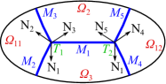
Figure 3.1. Disconnected triple junction partition for Example 6 and Proposition 7.

Example 6.

For the disconnected 3-phase partitioning of $\Omega$ (see Figure 3.1) by a system of two triple junctions, the modified area functional is given by

(3.8) $$A^{\star}(M)=A(T)-\lambda_{2}\left|\Omega_{2}\right|-\lambda_{3}\left|\Omega_{3}\right|$$

In this expression,

$$A(T)=\sum_{i=1}^{5}\gamma_{i}A(M_{i}),$$

$\gamma_{1}=\epsilon_{23}$, $\gamma_{2}=\gamma_{4}=\epsilon_{13}$, $\gamma_{3}=\gamma_{5}=\epsilon_{12}$, and $\epsilon_{ij}=\epsilon_{ji}$ is the interfacial energy density of the interface separating phases $i$, $j$. The volume constants $V_{j}$ were dropped as they play no part in the variational process. On using the volume constraints for phases 1 and 2, the modified area functional assumes the form

(3.9) $$A^{\star}(M)=A(T)-\lambda_{1}\left(\left|\Omega_{11}\right|+\left|\Omega_{12}\right|\right)-\lambda_{2}\left|\Omega_{2}\right|$$

We can also use all three constraints, which does not alter the final formulas and results. Occasionally, we use a notation indicating the triple junction, which an interface belongs to. In this notation the area functional becomes

$$A(T)=\sum_{p=1}^{3}\sum_{j=1}^{2}\gamma_{pj}A(M_{pj})$$

The indices $p$ and $j$ stand for “phase” and “junction”, $M_{pj}$ is the interface opposite to phase $p$ at junction $j$ (for example, in Figure 3.1 $M_{22}$ is shown as $M_{4}$) and $\gamma_{pj}$ the corresponding surface tension. Since there is only one interface between phases 2 and 3, $M_{11}\equiv M_{12}\equiv M_{1}$, and this term occurs only once in the sum. In a similar fashion, we drop superfluous indices from subsets. For example, referring to Figure 3.1, we write $\Omega_{2}$ and $\Omega_{3}$ instead of $\Omega_{21}$ and $\Omega_{31}$. The connection between notations is

(3.10) $$\begin{array}[]{cccccccc}M_{11}&\gamma_{11}&\leftrightarrow&M_{1}&\gamma_{1}&\leftrightarrow&M_{23}^{(1)}\equiv M_{23}^{(2)}&\epsilon_{23}\\ M_{21}&\gamma_{21}&\leftrightarrow&M_{2}&\gamma_{2}&\leftrightarrow&M_{13}^{(1)}&\epsilon_{13}\\ M_{31}&\gamma_{31}&\leftrightarrow&M_{3}&\gamma_{3}&\leftrightarrow&M_{12}^{(1)}&\epsilon_{12}\\ M_{22}&\gamma_{22}&\leftrightarrow&M_{4}&\gamma_{4}&\leftrightarrow&M_{13}^{(2)}&\epsilon_{13}\\ M_{32}&\gamma_{32}&\leftrightarrow&M_{5}&\gamma_{5}&\leftrightarrow&M_{12}^{(2)}&\epsilon_{12}\end{array}$$

The first two columns refer to the second notation, the next two to the first notation and the last two to the interfacial system (see Section 1, text below equation (1.1)). In the latter, $M_{pq}^{(j)}$ is the interface between phases $p,q$ attached to triple junction $j$. $\square$

The following theorem extends Proposition 5 to general disconnected triple junction partitions.

Proposition 7.

Let $T=(T_{j})_{j=1}^{r}=(M_{pj})_{p=1,\cdots,3;j=1,\cdots,r}$ be a three-phase partitioning of $\Omega\subset\mathbb{R}^{3}$ by a system of $r$ $C^{2}$-triple junctions, into the domains $\Omega_{pj}$ $(j=1,\cdots,r;p=1,2,3)$. Further let $N_{pj}$ be the unit normal field of $M_{pj}$ and $N_{\Sigma}$ be the unit normal field of $\Sigma$. If $T$ is minimal, then

(i) Young’s equality (3.2) holds for each triple junction in the system. Equivalently, the following equalities

(3.11) $$\sum_{p=1}^{3}\gamma_{pj}\nu_{pj}=0$$

hold for all triple junctions $j$ of the system.

(ii) The scalar mean curvature $\kappa_{pj}=H_{pj}\cdot N_{pj}$ of each interface $M_{pj}$ is constant and

(3.12) $$\kappa_{p1}=\cdots=\kappa_{pr}\equiv\kappa_{p}$$

for all $p=1,2,3$.

(iii) The scalar mean curvatures $\kappa_{p}$ satisfy the relation

(3.13) $$\sum_{p=1}^{3}\gamma_{p}\kappa_{p}=0$$

on each triple junction.

(iv) Each $M_{pj}$ is normal to $\Sigma$, i.e. on each $M_{pj}\cap\Sigma$ we have $N_{pj}\cdot N_{\Sigma}=0$ or $N_{pj}\in T\Sigma$.

Remark 8.

Equality (3.13) holds for each triple junction,

$$\sum_{p=1}^{3}\gamma_{pj}\kappa_{pj}=0$$

However, in view of (3.12) and the fact that $\gamma_{pj}=\gamma_{p}$ for all $j$ (see correspondence table (3.10)), all these equalities reduce to the single equality (3.13).

Proof.

For concreteness we consider the disconnected 3-phase partitioning of Fig. 3.1 with the indicated orientation. Letting $w$ be any variation of $T$, by (3.8) in view of (2.5) and (3.4) we obtain

$$\delta A^{\star}(T) =\sum_{j=1}^{2}\sum_{p=1}^{3}\gamma_{pj}\delta A(M_{pj})-\lambda_{2}\delta\left|\Omega_{2}\right|-\lambda_{3}\delta\left|\Omega_{3}\right|$$

$$=-\sum_{j=1}^{2}\sum_{p=1}^{3}\gamma_{pj}\int_{M_{pj}}H_{pj}\cdot w$$

$$+\sum_{j=1}^{2}\sum_{p=1}^{3}\gamma_{pj}\int_{S}\nu_{pj}\cdot w+\sum_{j=1}^{2}\sum_{p=1}^{3}\gamma_{pj}\int_{\partial M_{pj}\cap\Sigma}\nu_{pj}\cdot w$$

$$-\lambda_{2}\int_{M_{1}}N_{1}\cdot w-\lambda_{2}\int_{M_{31}}(-N_{31})\cdot w-\lambda_{2}\int_{M_{32}}(-N_{32})\cdot w$$

$$-\lambda_{3}\int_{M_{1}}(-N_{1})\cdot w-\lambda_{3}\int_{M_{21}}N_{21}\cdot w-\lambda_{3}\int_{M_{22}}N_{22}\cdot w$$

Rearranging gives

(3.14) $$\delta A^{\star}(T) =\int_{M_{1}}\left[\left(\lambda_{3}-\lambda_{2}\right)N_{1}-\gamma_{1}H_{1}\right]\cdot w$$

$$+\int_{M_{21}}\left(-\lambda_{3}N_{21}-\gamma_{21}H_{21}\right)\cdot w+\int_{M_{31}}\left(\lambda_{2}N_{31}-\gamma_{31}H_{31}\right)\cdot w$$

$$+\int_{M_{22}}\left(-\lambda_{3}N_{22}-\gamma_{22}H_{22}\right)\cdot w+\int_{M_{32}}\left(\lambda_{2}N_{32}-\gamma_{32}H_{32}\right)\cdot w$$

$$+\int_{S}\left(\sum_{j=1}^{2}\sum_{p=1}^{3}\gamma_{pj}\nu_{pj}\right)\cdot w+\sum_{j=1}^{2}\sum_{p=1}^{3}\gamma_{pj}\int_{\partial M_{pj}\cap\Sigma}\nu_{pj}\cdot w$$

Using variations concentrated on each leaf gives

(3.15) $$\begin{array}[]{l}-\gamma_{1}H_{1}\cdot N_{1}+\lambda_{3}-\lambda_{2}=0\\ -\gamma_{21}H_{21}\cdot N_{21}-\lambda_{3}=0\\ -\gamma_{31}H_{31}\cdot N_{31}+\lambda_{2}=0\\ -\gamma_{22}H_{22}\cdot N_{22}-\lambda_{3}=0\\ -\gamma_{32}H_{32}\cdot N_{32}+\lambda_{2}=0\end{array}$$

By (3.14), using variations concentrated on each spine, we obtain

(3.16) $$\sum_{p=1}^{3}\gamma_{pj}\nu_{pj}=0,\quad j=1,2$$

Variations concentrated on each $\partial M_{pj}\cap\Sigma$ give

(3.17) $$\nu_{pj}\cdot w=0$$

for $p,j$ such that $\partial M_{pj}\cap\Sigma\neq\emptyset$. From these relations it follows without difficulty that $\nu_{pj}\in N\Sigma$ and this proves (iv).

Part (i) follows from equations (3.16) by the same argumentation applied in the proof of Proposition 5. By the second and fourth of (3.15), on account of $\gamma_{21}=\gamma_{22}$ we obtain

$$\kappa_{21}=\kappa_{22}$$

and in a similar fashion from the third and fifth of (3.15)

$$\kappa_{31}=\kappa_{32}$$

The equality $\kappa_{11}=\kappa_{12}$ is trivial, and this proves (ii). The constancy of the $\kappa$’s follows immediately from (3.15). Addition of the first three equations of (3.15) gives $\sum_{p=1}^{3}\gamma_{p1}\kappa_{p1}=0$ and addition of the first, fourth and fifth gives $\sum_{p=1}^{3}\gamma_{p2}\kappa_{p2}=0$. By Remark 8 these are identical and this proves (iii). ∎

4. Second Variation Formulas

Formula (2.6) for the second variation of area is quite general but not directly applicable. Here we derive a more convenient expression for hypersurfaces with constant mean curvature, which in a subsequent step is applied to multijunction partitions. To satisfy the condition of fixed container walls, following [13], we define admissible variations by the solutions of the initial value problem

(4.1) $$\frac{d\xi}{dt}=w(\xi),\quad\xi(0)=x$$

Letting $\xi_{x}$ be the solution of (4.1) for the initial condition $\xi_{x}(0)=x$, we set $\xi(x,t)=\xi_{x}(t)$ for the corresponding variation. For solid undeformable walls we choose $w$ so that $w(p)\in T_{p}\Sigma$ for any $p\in\Sigma=\partial\Omega$.

On taking the time derivative of (4.1) we obtain the following expression for the second variation field:

(4.2) $$a=D_{w}w$$

Proposition 9.

Let $M$ be $C^{2}$-hypersurface of $\mathbb{R}^{n}$ with boundary. We assume that $M$ has constant mean curvature $\kappa$ and $w$ is a variation compactly supported in $M$ and whose support is contained in a chart of $M$. Further let $N$ be the unit normal field of $M$ in a chart containing the support of $w$, $\nu$ the unit outward normal of $\partial M$ which is tangent to $M$, $u=w^{\top}$, $v=w^{\bot}$, and $f=w\cdot N$. Then the second variation of the area of $M$ is given by

(4.3) $$\delta^{2}A(M)= \int_{M}\left(|\mathrm{grad}_{M}f|^{2}-|B_{M}|^{2}f^{2}\right)+$$

$$\int_{M}\kappa\left[II_{M}(u,u)-2f\mathrm{div}_{M}u+\kappa f^{2}-a\cdot N\right]+$$

$$\int_{\partial M}\left[(u\cdot\nu)\mathrm{div}_{M}u-\left\langle\nabla_{u}u,\nu\right\rangle+2fII_{M}(u,\nu)+a\cdot\nu\right]$$

and for variations satisfying (4.1)

(4.4) $$\delta^{2}A(M)= \int_{M}\left(|\mathrm{grad}_{M}\,f\,|^{2}-|B_{M}|^{2}f^{2}\right)+$$

$$\int_{M}\kappa\left[II_{M}(u,u)-2f\mathrm{div}_{M}u+\kappa f^{2}-a\cdot N\right]+$$

$$\int_{\partial M}\left[(u\cdot\nu)\mathrm{div}_{M}u+fII_{M}(u,\nu)+f\left\langle D_{N}w,\nu\right\rangle\right]$$

where

$$|B_{M}|^{2}=g^{ik}g^{jl}B_{ij}B_{kl}=B_{j}^{i}B_{i}^{j},\quad B_{ij}=II_{M}(E_{i},E_{j}),$$

and $\left(E_{i}(p)\right)_{i=1}^{n-1}$ is a local basis of $T_{p}M$.

Proof.

To perform the calculations in an orderly fashion we set

$$I:=g^{ij}\left\langle(D_{E_{i}}w)^{\bot},(D_{E_{j}}w)^{\bot}\right\rangle$$

$$J:=g^{ik}g^{jl}\left\langle(D_{E_{i}}w)^{\top},E_{j}\right\rangle\left\langle(D_{E_{l}}w)^{\top},E_{k}\right\rangle$$

$$K:=\mathrm{div}_{M}a,\quad L:=(\mathrm{div}_{M}w)^{2}.$$

Then, noticing that all these items are bilinear in $w$ (for $K$ this will become clear shortly), we name the terms resulting from breaking $w$ into tangent and normal parts, by adding the indices $n$ and $t$ denoting normal and tangent parts respectively. For example, for $I$ we have $I=I_{tt}+I_{tn}+I_{nt}+I_{tt}$, where $I_{tt}=g^{ij}\left\langle(D_{E_{i}}u)^{\bot},(D_{E_{j}}u)^{\bot}\right\rangle$, $I_{tn}=g^{ij}\left\langle(D_{E_{i}}u)^{\bot},(D_{E_{j}}v)^{\bot}\right\rangle$ etc.

Using this notation, the generic formula for the second variation of area (2.6) reads

(4.5) $$\delta^{2}A(M) =\int_{M}(K+L+I_{tt}+2I_{tn}+I_{nn}-J_{tt}-2J_{tn}-J_{nn})$$

$$=\int_{M}\left[(I_{nn}-J_{nn})+2(I_{tn}-J_{tn})+(L+I_{tt}-J_{tt})+K\right].$$

Since calculations are often done more conveniently in coordinate notation, while final results are more concisely expressed coordinate-free, we give all items in both notations. We are using summation convention throughout. From

(4.6) $$D_{E_{i}}v=D_{E_{i}}(fN)=fD_{E_{i}}N+(D_{E_{i}}f)N$$

recalling that $D_{E_{i}}N\in TM$ we obtain

(4.7) $$(D_{E_{i}}v)^{\bot}=(D_{E_{i}}f)N=\frac{\partial f}{\partial q^{i}}N$$

where $q^{1},q^{2},\cdots,q^{n-1}$ is a local coordinate system of $M$. We are using the same notation for $f:M\to\mathbb{R}$ and $f\circ\mathbf{x}$, $\mathbf{x}$ being a parametrization (inverse chart mapping) of $M$. By (4.7)

(4.8) $$I_{nn}:=g^{ij}\left\langle(D_{E_{i}}v)^{\bot},(D_{E_{j}}v)^{\bot}\right\rangle=g^{ij}\frac{\partial f}{\partial q^{i}}\frac{\partial f}{\partial q^{j}}=\left|\mathrm{grad}_{M}f\right|^{2}$$

Since $u\cdot N=0$ and $\dim N_{p}M=1$ $(p\in M)$,

$$I_{tt} =g^{ij}\left\langle(D_{E_{i}}u)^{\bot},(D_{E_{j}}u)^{\bot}\right\rangle=g^{ij}\left\langle(D_{E_{i}}u)^{\bot},N\right\rangle\left\langle(D_{E_{j}}u)^{\bot},N\right\rangle$$

$$=g^{ij}\left\langle D_{E_{i}}u,N\right\rangle\left\langle D_{E_{j}}u,N\right\rangle=g^{ij}\left\langle u,D_{E_{i}}N\right\rangle\left\langle u,D_{E_{j}}N\right\rangle$$

By the definition of the Weingarten mapping,

(4.9) $$I_{tt}=|Wu|^{2}=B_{ki}B_{\,j}^{k}u^{i}u^{j}.$$

Here $u^{1},\cdots,u^{n-1}$ are the components of $u$ in the coordinate system $q^{1},\cdots,q^{n-1}$, $B_{ij}=II_{M}(E_{i},E_{j})$ the components of the 2nd fundamental form and $B_{\,j}^{i}=g^{ik}B_{kj}$ the corresponding mixed contravariant-covariant components. In the derivation of (4.9) the following identity was used

(4.10) $$D_{E_{i}}N=WE_{i}=-B_{\,i}^{k}E_{k}.$$

By (4.7) and the definition of the Weingarten mapping we obtain

$$I_{tn} =g^{ij}\left\langle(D_{E_{i}}u)^{\bot},(D_{E_{j}}v)^{\bot}\right\rangle=g^{ij}\left\langle D_{E_{i}}u,(D_{E_{j}}v)^{\bot}\right\rangle$$

$$=g^{ij}\frac{\partial f}{\partial q^{j}}\left\langle D_{E_{i}}u,N\right\rangle=-g^{ij}\frac{\partial f}{\partial q^{j}}\left\langle u,D_{E_{i}}N\right\rangle$$

$$=-\left\langle u,D_{\mathrm{grad}_{M}f}N\right\rangle=-\left\langle u,W\mathrm{grad}_{M}f\right\rangle$$

By the self-adjointness of the Weingarten mapping and (4.10) we obtain the following alternative expressions for $I_{tn}$:

(4.11) $$I_{tn}=-\left\langle Wu,\mathrm{grad}_{M}f\right\rangle=II_{M}(u,\mathrm{grad}_{M}f)=B_{\,i}^{j}u^{i}\frac{\partial f}{\partial q^{j}}.$$

It is easily checked that $I_{tn}=I_{nt}$.

We proceed to the calculation of $J$-terms. Recalling the definition of covariant derivative from Section 2 and its component notation $\nabla_{Y}X=X_{|k}^{i}Y^{k}E_{i}$, $X,Y\in TM$, we have

$$J_{tt}=g^{ik}g^{jl}\left\langle(D_{E_{i}}u)^{\top},E_{j}\right\rangle\left\langle(D_{E_{l}}u)^{\top},E_{k}\right\rangle=u_{\,|i}^{k}u_{\,|k}^{i}$$

On using the following notation for the double contraction of two tensors $S,T$

$$S:T=S_{\,j}^{i}T_{\,i}^{j}$$

we obtain

(4.12) $$J_{tt}=u_{\,|i}^{k}u_{\,|k}^{i}=\nabla u:\nabla u$$

By (4.6)

$$J_{tn} =g^{ik}g^{jl}\left\langle(D_{E_{i}}u)^{\top},E_{j}\right\rangle\left\langle(D_{E_{l}}v)^{\top},E_{k}\right\rangle$$

$$=g^{ik}g^{jl}\left\langle\nabla_{E_{i}}u,E_{j}\right\rangle\left\langle fD_{E_{l}}N,E_{k}\right\rangle$$

$$=-fg^{ik}g^{jl}\left\langle u_{\,|i}^{r}E_{r},E_{j}\right\rangle II_{M}(E_{l},E_{k})$$

$$=-fg^{ik}u_{\,|i}^{l}B_{lk}=-fu_{\,|i}^{l}B_{\,l}^{i}$$

and

(4.13) $$J_{tn}=-fu_{\,|i}^{l}B_{\,l}^{i}=-fII_{M}:\nabla u$$

The symmetry $J_{tn}=J_{nt}$ follows immediately by interchanging indices $i\leftrightarrow l$, $j\leftrightarrow k$. Again by (4.6)

$$J_{nn} =g^{ik}g^{jl}\left\langle(D_{E_{i}}v)^{\top},E_{j}\right\rangle\left\langle(D_{E_{l}}v)^{\top},E_{k}\right\rangle$$

$$=f^{2}g^{ik}g^{jl}\left\langle D_{E_{i}}N,E_{j}\right\rangle\left\langle D_{E_{l}}N,E_{k}\right\rangle$$

$$=f^{2}g^{ik}g^{jl}\left\langle N,D_{E_{i}}E_{j}\right\rangle\left\langle N,D_{E_{l}}E_{k}\right\rangle=f^{2}B_{\,i}^{k}B_{\,k}^{i}$$

and

(4.14) $$J_{nn}=f^{2}B_{\,i}^{k}B_{\,k}^{i}=f^{2}|B_{M}|^{2}.$$

By (see [17])

(4.15) $$\mathrm{div}_{M}w=\mathrm{div}_{M}u-H\cdot v$$

since $M$ was supposed to have constant mean curvature $\kappa=H\cdot N$, we obtain $\mathrm{div}_{M}w=\mathrm{div}_{M}u-\kappa f$ and from this

(4.16) $$(\mathrm{div}_{M}w)^{2}=(\mathrm{div}_{M}u)^{2}-2\kappa f\mathrm{div}_{M}u+\kappa^{2}f^{2}$$

After this preparation we are ready to calculate the right side of (4.5). By (4.11), (4.13) and the properties of covariant derivative we obtain

$$I_{tn}-J_{tn} =B_{\,i}^{j}u^{i}\frac{\partial f}{\partial q^{j}}+fu_{\,|j}^{i}B_{\,i}^{j}=B_{\,i}^{j}(fu^{i})_{|j}$$

(4.17) $$=(fB_{\,i}^{j}u^{i})_{|j}-fu^{i}B_{\,i|j}^{j}$$

We will prove that for a hypersurface with constant mean curvature

(4.18) $$B_{\,i|j}^{j}=0.$$

By the Mainardi-Codazzi equations in component form

$$B_{jk|i}=B_{ik|j}$$

and Ricci’s lemma, we obtain

$$B_{\,j|i}^{k}=B_{\,i|j}^{k}$$

and from this by contraction over the indices $i$, $k$

(4.19) $$B_{\,j|i}^{i}=B_{\,i|j}^{i}.$$

The Mainardi-Codazzi equations in component form were obtained from their component-free version ([19], vol. III, p. 10),

$$(\nabla_{X}II)(Y,Z)=(\nabla_{Y}II)(X,Z)$$

by setting $X=E_{i}$, $Y=E_{j}$, $Z=E_{k}$ and recalling that

$$(\nabla_{E_{i}}II)(E_{j},E_{k})=B_{jk|i}.$$

By the definition of mean curvature (2.2) and equations (2.1) and (2.3),

(4.20) $$\kappa=B_{\,i}^{i}.$$

Since $\kappa$ is constant by hypothesis, application of (4.19) yields (4.18), and with this (4.17) reduces to

(4.21) $$I_{tn}-J_{tn}=(fB_{\,i}^{j}u^{i})_{|j}=-\mathrm{div}_{M}(fWu)$$

We calculate the third item under the integral sign on the right side of (4.5). By (4.16) and (4.12) we have

(4.22) $$L-J_{tt}=(u_{\,i}^{i}u^{j}-u^{i}u_{\,|i}^{j})_{|j}+u^{i}(u_{\,|ij}^{j}-u_{\,ji}^{j})-2\kappa f\mathrm{div}_{M}u+\kappa^{2}f^{2}$$

(4.23) $$L-J_{tt} =u_{\,|i}^{i}u_{\,|j}^{j}-u_{\,|j}^{i}u_{\,|i}^{j}-2\kappa fu_{\,|i}^{i}+\kappa^{2}f^{2}$$

$$=(u_{\,|i}^{i}u^{j}-u^{i}u_{\,|i}^{j})_{|j}-u^{j}u_{\,|ij}^{i}+u^{i}u_{\,|ij}^{j}-2\kappa fu_{\,|i}^{i}+\kappa^{2}f^{2}$$

$$=(u_{\,|i}^{i}u^{j}-u^{i}u_{\,|i}^{j})_{|j}+u^{i}(u_{\,|ij}^{j}-u_{\,|ji}^{j})-2\kappa fu_{\,|i}^{i}+\kappa^{2}f^{2}$$

By Ricci’s identity (see [19], vol. II, p. 224),

$$u_{\,|ij}^{r}-u_{\,|ji}^{r}=R_{\,kji}^{r}u^{k}$$

on contracting upon the indices $r,i$

$$u_{\,|ij}^{i}-u_{\,|ji}^{i}=R_{\,kji}^{i}u^{k}=R_{kj}u^{k}$$

and renaming indices, we obtain

(4.24) $$u_{\,|ij}^{j}-u_{\,|ji}^{j}=-R_{ki}u^{k}$$

In these equalities

$$R_{jk}=R_{\,jki}^{i}=g^{ri}R_{rjki}$$

are the components of Ricci’s tensor and

$$R_{ijkl}=\left\langle R(E_{k},E_{l})E_{j},E_{i}\right\rangle$$

are the components of the curvature tensor ([19], vol. II, pp. 190, 239). By Gauss’ Theorema Egregium ([19], vol III, p. 5, Theorem 6) we have

$$\left\langle R(E_{k},E_{l})E_{j},E_{i}\right\rangle=B_{ik}B_{jl}-B_{il}B_{jk}$$

hence

(4.25) $$R_{jk}=g^{il}B_{ik}B_{jl}-B_{\,i}^{i}B_{jk}.$$

Since $M$ has constant mean curvature, by (4.20) it follows that

(4.26) $$R_{jk}=g^{rs}B_{rj}B_{sk}-\kappa B_{jk}$$

Using this equality in (4.24) gives

(4.27) $$u^{i}(u_{\,|ij}^{j}-u_{\,|ji}^{j})=-g^{rs}B_{ri}B_{sk}u^{i}u^{k}+\kappa B_{ik}u^{i}u^{k}$$

Combination of (4.23), (4.27) and (4.9) yields

(4.28) $$L+I_{tt}-J_{tt} =\mathrm{div}_{M}\left(u\mathrm{div}_{M}u-\nabla_{u}u\right)$$

$$+\kappa II_{M}(u,u)-2\kappa f\mathrm{div}_{M}u+\kappa^{2}f^{2}$$

On using (4.28), (4.21), (4.8) and (4.14) in (4.5) we obtain

$$\delta^{2}A(M) =\int_{M}\left(|\mathrm{grad}_{M}f|^{2}-|B_{M}|^{2}f^{2}\right)$$

$$-2\int_{M}\mathrm{div}_{M}(fWu)+\int_{M}\mathrm{div}_{M}\left(u\mathrm{div}_{M}u-\nabla_{u}u\right)$$

$$+\int_{M}\kappa\left[II_{M}(u,u)-2f\mathrm{div}_{M}u+\kappa f^{2}\right]+\int_{M}\left(\mathrm{div}_{M}a^{\top}-H\cdot a^{\bot}\right)$$

Application of the divergence theorem gives

$$\delta^{2}A(M) =\int_{M}\left(|\mathrm{grad}_{M}f|^{2}-|B_{M}|^{2}f^{2}\right)$$

$$+\int_{M}\kappa\left[II_{M}(u,u)-2f\mathrm{div}_{M}u+\kappa f^{2}-a\cdot N\right]$$

$$-2\int_{\partial M}f\left\langle Wu,\nu\right\rangle+\int_{\partial M}\left[(u\cdot\nu)\mathrm{div}_{M}u-\left\langle\nabla_{u}u,\nu\right\rangle\right]+\int_{\partial M}a\cdot\nu$$

From this, equality (4.3) follows immediately from

(4.29) $$\left\langle Wu,\nu\right\rangle=-II_{M}(u,\nu).$$

Formula (4.4) follows by Lemma 10 below. ∎

Lemma 10.

For a variation of type (4.1) the second variation field $a$ satisfies the following equality

(4.30) $$\int_{M}\mathrm{div}_{M}a^{\top}=\int_{\partial M}\left(f\left\langle D_{N}w,\nu\right\rangle-fII_{M}(u,\nu)+\left\langle\nabla_{u}u,\nu\right\rangle\right)$$

Proof.

Application of the divergence theorem to (4.1) gives

(4.31) $$\int_{M}\mathrm{div}_{M}a^{\top}=\int_{\partial M}\left\langle D_{w}w,\nu\right\rangle=\int_{\partial M}f\left\langle D_{N}w,\nu\right\rangle+\int_{\partial M}\left\langle D_{u}w,\nu\right\rangle.$$

By the decomposition $w=u+v$ and

(4.32) $$\left\langle D_{u}v,\nu\right\rangle=-\left\langle v,D_{u}\nu\right\rangle=-fII_{M}(u,\nu)$$

we obtain (4.30). ∎

Lemma 11.

Let $T=(T_{j})_{j=1}^{r}$, $T_{j}=(M_{pj})_{p=1}^{3}$, be a three phase partitioning of a domain $\Omega\subset\mathbb{R}^{n}$ by a system of $r$ $C^{2}$-triple junctions into the domains $\Omega_{pj}$ $(p=1,\cdots,3;j=1,\cdots,r)$. Let $\tilde{\Omega}=\Omega_{pj}$ be any one of these domains. Then, for variations $w$ of type (4.1) preserving $\Sigma$, the second variation of volume of $\tilde{\Omega}$ is given by

(4.33) $$\delta^{2}|\tilde{\Omega}|=\int_{\partial\tilde{\Omega}\backslash\Sigma}(w\cdot N_{\partial\tilde{\Omega}})\mathrm{div}_{\mathbb{R}^{n}}w$$

where $N_{\partial\tilde{\Omega}}$ is the unit outward normal of $\tilde{\Omega}$.

Proof.

If $(\xi^{t})_{t\in I}$ is a variation with first variation field $w$, and $\tilde{\Omega}^{t}=\xi^{t}(\tilde{\Omega})$, we have

$$|\tilde{\Omega}^{t}|=\int_{\xi^{t}(\tilde{\Omega})}dx=\int_{\tilde{\Omega}}J\xi^{t}(y)dy$$

where $J\xi^{t}$ is the Jacobian of $\xi^{t}$. For the second variation of this functional we have

$$\delta^{2}|\tilde{\Omega}|=\left.\frac{d^{2}}{dt^{2}}|\tilde{\Omega}^{t}|\right|_{t=0}=\int_{\tilde{\Omega}}\left.\frac{\partial^{2}}{\partial t^{2}}J\xi^{t}(y)\right|_{t=0}dy.$$

Application of the rule of determinant differentiation and straight-forward manipulations give

$$\left.\frac{\partial^{2}}{\partial t^{2}}J\xi^{t}(y)\right|_{t=0}=\mathrm{div}_{\mathbb{R}^{n}}a+\frac{\partial w^{\alpha}}{\partial x^{\alpha}}\frac{\partial w^{\beta}}{\partial x^{\beta}}-\frac{\partial w^{\alpha}}{\partial x^{\beta}}\frac{\partial w^{\beta}}{\partial x^{\alpha}}.$$

We are using Greek indices for vector components and coordinates in the surrounding space $\mathbb{R}^{n}$ and Latin for the manifold $M$. Summation convention applies to Greek indices as well. Formula (4.33) follows from this equality, the identity

$$\frac{\partial w^{\alpha}}{\partial x^{\alpha}}\frac{\partial w^{\beta}}{\partial x^{\beta}}-\frac{\partial w^{\alpha}}{\partial x^{\beta}}\frac{\partial w^{\beta}}{\partial x^{\alpha}} =\frac{\partial}{\partial x^{\alpha}}\left(w^{\alpha}\frac{\partial w^{\beta}}{\partial x^{\beta}}-w^{\beta}\frac{\partial w^{\alpha}}{\partial x^{\beta}}\right)$$

$$=\mathrm{div}_{\mathbb{R}^{n}}\left(w\mathrm{div}_{\mathbb{R}^{n}}w-D_{w}w\right)$$

and Gauss’ theorem, in view of (4.2). The hypothesis that the variation preserves $\Sigma$ is only used to drop the integral over $\partial\tilde{\Omega}\cap\Sigma$. ∎

On the basis of the above results, in the next theorem we develop a formula for the second variation of area for minimal triple junction partitions with volume constraints.

Theorem 12.

Let $\Omega$ be a domain in $\mathbb{R}^{3}$, $T=(T_{j})_{j=1}^{r}$, $T_{j}=(M_{pj})_{p=1}^{3}$, a minimal three-phase partition of $\Omega$ by a set of $r$ $C^{2}$ triple junctions with volume constraints, and $w$ an admissible variation satisfying (4.1) and the volume constraints. On each leaf $M_{pj}$ we have the splitting $w=u_{pj}+v_{pj}$, $u_{pj}\in TM_{pj}$, $v_{pj}\in NM_{pj}$, and we set $f_{pj}=w\cdot N_{pj}=v_{pj}\cdot N_{pj}$, $N_{pj}$ being the unit normal field of $M_{pj}$. Then the following formula holds for the second variation of the area functional,

(4.34) $$\begin{gathered}\delta^{2}A^{\star}(T)=\sum_{p,j}\gamma_{pj}\int_{M_{pj}}\left(|\mathrm{grad}_{M_{pj}}f_{pj}|^{2}-|B_{M_{pj}}|^{2}f_{pj}^{2}\right)\\ -\sum_{j=1}^{r}\sum_{p=1}^{3}\gamma_{pj}\int_{\partial M_{pj}\cap\varSigma}f_{pj}^{2}II_{\varSigma}(N_{pj},N_{pj})\\ +\sum_{j=1}^{r}\sum_{p=1}^{3}\gamma_{pj}\int_{S_{j}}f_{pj}h_{pj}II_{M_{pj}}(\nu_{pj},\nu_{pj})\end{gathered}$$

where $S_{j}$ is the spine of $T_{j}$ and $\nu_{pj}\in TM_{pj}$ is the unit normal field of $\partial M_{pj}\cap S_{j}$.

Proof.

The second variation of the area functional with Lagrange multipliers, equation (3.7), is given by

$$\delta^{2}A^{\star}(M)=\delta^{2}A(M)-\sum_{j=2}^{3}\lambda_{j}\sum_{k=1}^{P_{j}}\delta^{2}\left|\Omega_{jk}\right|$$

Again, for concreteness and to keep the length of formulas to a minimum, we consider the disconnected three phase partitioning of Figure 3.1 with the indicated orientation. For this configuration the area functional is given by (3.7). Use of (4.33) gives

$$\delta^{2}A^{\star}(M) =\sum_{j=1}^{2}\sum_{p=1}^{3}\gamma_{pj}\delta^{2}A(M_{pj})-\lambda_{2}\delta^{2}\left|\Omega_{2}\right|-\lambda_{3}\delta^{2}\left|\Omega_{3}\right|$$

$$=\sum_{j=1}^{2}\sum_{p=1}^{3}\gamma_{pj}\delta^{2}A(M_{pj})-(\lambda_{2}-\lambda_{3})\int_{M_{1}}w\cdot N_{1}\,\mathrm{div}_{\mathbb{R}^{3}}w$$

$$-\lambda_{2}\int_{M_{31}}w\cdot(-N_{31})\mathrm{div}_{\mathbb{R}^{3}}w-\lambda_{2}\int_{M_{32}}w\cdot(-N_{32})\mathrm{div}_{\mathbb{R}^{3}}w$$

$$-\lambda_{3}\int_{M_{21}}w\cdot N_{21}\,\mathrm{div}_{\mathbb{R}^{3}}w-\lambda_{3}\int_{M_{22}}w\cdot N_{22}\,\mathrm{div}_{\mathbb{R}^{3}}w$$

By equations (3.15) and $\kappa_{pj}=H_{pj}\cdot N_{pj}$ (see Proposition 7(ii)) we obtain

$$\delta^{2}A^{\star}(M) =\sum_{j=1}^{2}\sum_{p=1}^{3}\gamma_{pj}\delta^{2}A(M_{pj})+\gamma_{1}\kappa_{1}\int_{M_{1}}w\cdot N_{1}\,\mathrm{div}_{\mathbb{R}^{3}}w$$

$$+\gamma_{31}\kappa_{31}\int_{M_{31}}w\cdot N_{31}\,\mathrm{div}_{\mathbb{R}^{3}}w+\gamma_{32}\kappa_{32}\int_{M_{32}}w\cdot N_{32}\,\mathrm{div}_{\mathbb{R}^{3}}w$$

$$+\gamma_{21}\kappa_{21}\int_{M_{21}}w\cdot N_{21}\,\mathrm{div}_{\mathbb{R}^{3}}w+\gamma_{22}\kappa_{22}\int_{M_{22}}w\cdot N_{22}\,\mathrm{div}_{\mathbb{R}^{3}}w$$

Each term of the double sum on the right side corresponds to one integral, and thus we can express $\delta^{2}A^{\star}(M)$ as follows:

$$\delta^{2}A^{\star}(M)=\sum_{j=1}^{2}\sum_{p=1}^{3}\gamma_{pj}\left[\delta^{2}A(M_{pj})+\kappa_{pj}\int_{M_{pj}}w\cdot N_{pj}\,\mathrm{div}_{\mathbb{R}^{3}}w\right]$$

We set

$$\delta^{2}A^{\star}(M_{pj})=\delta^{2}A(M_{pj})+\kappa_{pj}\int_{M_{pj}}w\cdot N_{pj}\,\mathrm{div}_{\mathbb{R}^{3}}w$$

so that

$$\delta^{2}A^{\star}(M)=\sum_{j}\sum_{p=1}^{3}\gamma_{pj}\delta^{2}A^{\star}(M_{pj}).$$

Using formula (4.3) of Proposition 9 gives for $\delta^{2}A^{\star}(M_{pj})$

$$\delta^{2}A^{\star}(M_{pj}) =\int_{M_{pj}}\left(|\mathrm{grad}_{M_{pj}}f|^{2}-|B_{M_{pj}}|^{2}f^{2}\right)$$

$$+\int_{M_{pj}}\kappa_{pj}\left[II_{M_{pj}}(u,u)-2f\mathrm{div}_{M_{pj}}u+\kappa_{pj}f^{2}-a\cdot N_{pj}\right]$$

$$+\int_{\partial M_{pj}}\left[(u\cdot\nu)\mathrm{div}_{M_{pj}}u-\left\langle\nabla_{u}u,\nu\right\rangle+2fII_{M_{pj}}(u,\nu)+a\cdot\nu\right]$$

$$+\kappa_{pj}\int_{M_{pj}}w\cdot N_{pj}\,\mathrm{div}_{\mathbb{R}^{3}}w$$

and reordering terms,

(4.35) $$\delta^{2}A^{\star}(M_{pj}) =\int_{M_{pj}}\left(|\mathrm{grad}_{M_{pj}}f|^{2}-|B_{M_{pj}}|^{2}f^{2}\right)$$

$$+\int_{M_{pj}}\kappa_{pj}\left[II_{M_{pj}}(u,u)-2f\mathrm{div}_{M_{pj}}u+\kappa_{pj}f^{2}\right]$$

$$+\int_{\partial M_{pj}}\left[(u\cdot\nu)\mathrm{div}_{M_{pj}}u-\left\langle\nabla_{u}u,\nu\right\rangle+2fII_{M_{pj}}(u,\nu)\right.$$

$$\left.\qquad\qquad+a\cdot\nu\right]$$

$$+\int_{M_{pj}}\kappa_{pj}\left[-\left\langle D_{w}w,N_{pj}\right\rangle+\left(w\cdot N_{pj}\right)\,\mathrm{div}_{\mathbb{R}^{3}}w\right]$$

We treat the last two items under the integral sign in the last line. For brevity we drop the indices $p,j$ on $N_{pj}$ and $M_{pj}$. Substituting $w=u+v$, $v=fN$ and expanding, we obtain

$$\left\langle D_{w}w-(\mathrm{div}_{\mathbb{R}^{n}}w)w,N\right\rangle =\left\langle D_{u}u,N\right\rangle+\left\langle D_{u}v,N\right\rangle+\left\langle D_{v}u,N\right\rangle$$

$$+\left\langle D_{v}v,N\right\rangle-f\mathrm{div}_{\mathbb{R}^{n}}w$$

$$=II_{M}(u,u)+\left\langle fD_{u}N+(D_{u}f)N,N\right\rangle$$

$$+f\left\langle D_{N}u,N\right\rangle+f\left\langle D_{N}v,N\right\rangle$$

$$-f\mathrm{div}_{\mathbb{R}^{n}}v-f\mathrm{div}_{\mathbb{R}^{n}}u$$

By the identity

$$\mathrm{div}_{\mathbb{R}^{n}}X=\mathrm{div}_{M}X+\left\langle D_{N}X,N\right\rangle$$

and dropping canceling terms we obtain

(4.36) $$\left\langle D_{w}w-(\mathrm{div}_{\mathbb{R}^{n}}w)w,N\right\rangle=II_{M}(u,u)+\left\langle u,\mathrm{grad}_{M}f\right\rangle-f\mathrm{div}u+\kappa f^{2}$$

Combination of (4.35) and (4.36) gives

$$\delta^{2}A^{\star}(M_{pj}) =\int_{M_{pj}}\left(|\mathrm{grad}_{M_{pj}}f|^{2}-|B_{M_{pj}}|^{2}f^{2}\right)$$

$$+\int_{\partial M_{pj}}\left\langle u\mathrm{div}u-\nabla_{u}u-2fWu-\kappa_{pj}fu+a,\nu\right\rangle$$

Use of equation (4.30) and simplification gives

$$\delta^{2}A^{\star}(M_{pj}) =\int_{M_{pj}}\left(|\mathrm{grad}_{M_{pj}}f|^{2}-|B_{M_{pj}}|^{2}f^{2}\right)$$

$$+\int_{\partial M_{pj}}\left\langle u\mathrm{div}u-fWu-\kappa_{pj}fu+fD_{N_{pj}}w,\nu\right\rangle$$

We break integrals over $\partial M$ (again for brevity we drop indices on leaves and related quantities) into integrals over $\partial M\cap\varSigma$ and $\partial M\cap\Omega=S$, where $S$ is the spine of the triple junction $M$ belongs to. Since by minimality $u\cdot\nu=0$ (see equation (3.17)),

(4.37) $$\begin{gathered}\int_{\partial M}\left[fII_{M}(u,\nu)+\left(\mathrm{div}u-\kappa f\right)\left\langle u,\nu\right\rangle+f\left\langle D_{N}w,\nu\right\rangle\right]=\\ \int_{S}\left[fII_{M}(u,\nu)+\left(\mathrm{div}u-\kappa f\right)\left\langle u,\nu\right\rangle+f\left\langle D_{N}w,\nu\right\rangle\right]\\ +\int_{\partial M\cap\varSigma}f\left[II_{M}(u,\nu)+\left\langle D_{N}w,\nu\right\rangle\right]\end{gathered}$$

Let $\tau$ be a unit tangent field of $\partial M\cap\varSigma$. The triple $\nu,\tau,N$ makes up an orthonormal frame along $\partial M\cap\varSigma$. Since $u\cdot\nu=u\cdot N=0$ on $\partial M\cap\varSigma$, there is a $C^{1}$ function $g:\partial M\cap\varSigma\to\mathbb{R}$ such that $u=g\tau$ on $\partial M\cap\varSigma$, and as a consequence of this and $w\cdot\nu=u\cdot\nu=0$, we have $w=fN+g\tau$ on $\partial M\cap\varSigma$. Thus, for the boundary part of the above integral we have

(4.38) $$\begin{gathered}\int_{\partial M\cap\varSigma}f\left[II_{M}(u,\nu)+\left\langle D_{N}w,\nu\right\rangle\right]=\\ \int_{\partial M\cap\varSigma}fII_{M}(u,\nu)-\int_{\partial M\cap\varSigma}f\left\langle w,D_{N}\nu\right\rangle=\\ \int_{\partial M\cap\varSigma}fgII_{M}(\tau,\nu)-\int_{\partial M\cap\varSigma}f^{2}\left\langle N,D_{N}\nu\right\rangle-\int_{\partial M\cap\varSigma}fg\left\langle\tau,D_{N}\nu\right\rangle\end{gathered}$$

Let $N_{\varSigma}$ be the inward pointing unit normal field of $\varSigma$. By

$$II_{M}(\tau,\nu)=\left\langle D_{\tau}\nu,N\right\rangle=-\left\langle\nu,D_{\tau}N\right\rangle=\left\langle N_{\Sigma},D_{\tau}N\right\rangle=II_{\Sigma}(\tau,N),$$

since $\tau,N\in T\Sigma$, and

$$\left\langle\tau,D_{N}\nu\right\rangle=-\left\langle\tau,D_{N}N_{\varSigma}\right\rangle=\left\langle D_{N}\tau,N_{\varSigma}\right\rangle=II_{\varSigma}(\tau,N),$$

the first and last term on the last row of (4.38) cancel out, and we obtain

$$\begin{gathered}\int_{\partial M\cap\varSigma}f\left[II_{M}(u,\nu)+\left\langle D_{N}w,\nu\right\rangle\right]=\int_{\partial M\cap\varSigma}f^{2}\left\langle D_{N}N,\nu\right\rangle\\ =-\int_{\partial M\cap\varSigma}f^{2}II_{\varSigma}(N,N).\end{gathered}$$

Multiplication by $\gamma_{pj}$ and summation over the possible values of $p,j$ (i.e. over the leaves intersecting the boundary of $\Omega$) gives the first term on the second row of (4.34).

Finally, we treat the integral over the spine $S$ in (4.37). Recall that we are dropping leaf indices, and $\mathrm{div}u-\kappa f=\mathrm{div}_{M}w$. We consider as previously the unit tangent field $\tau$ of $S$, so that the triple $\nu,\tau,N$ makes up an orthonormal frame along $S$. Again, there are $C^{1}$ functions $h,g:S\to\mathbb{R}$ such that $u=h\nu+g\tau$ on $S$, and as a consequence of this, $w=fN+h\nu+g\tau$ on $S$. From the identities

$$\mathrm{div}_{M}w=\mathrm{div}_{\mathbb{R}^{3}}w-\left\langle D_{N}w,N\right\rangle$$

$$\mathrm{div}_{S}w=\mathrm{div}_{\mathbb{R}^{3}}w-\left\langle D_{N}w,N\right\rangle-\left\langle D_{\nu}w,\nu\right\rangle$$

we obtain

$$\mathrm{div}_{M}w=\mathrm{div}_{S}w+\left\langle D_{\nu}w,\nu\right\rangle.$$

Using this equality, the quantity under the integral sign over $S$ on the second row of (4.37) assumes the form

$$(u\cdot\nu)\mathrm{div}_{M}w+fII_{M}(u,\nu)+f\left\langle D_{N}w,\nu\right\rangle=$$

$$(w\cdot\nu)\mathrm{div}_{S}w+\left\langle D_{\nu}w,\nu\right\rangle h+fII_{M}(u,\nu)+\left\langle D_{v}w,\nu\right\rangle=$$

$$(w\cdot\nu)\mathrm{div}_{S}w+\left\langle D_{w}w,\nu\right\rangle-g\left\langle D_{\tau}w,\nu\right\rangle+fII_{M}(u,\nu)=$$

$$(w\cdot\nu)\mathrm{div}_{S}w+\left\langle D_{w}w,\nu\right\rangle-g\left\langle D_{\tau}w,\nu\right\rangle+fhII_{M}(\nu,\nu)+fgII_{M}(\tau,\nu)$$

Multiplication by $\gamma_{pj}$ and summation over the leaves of $T_{j}$, in view of (3.11) gives

(4.39) $$\sum_{p=1}^{3}\gamma_{pj}f_{pj}h_{pj}II_{M_{pj}}(\nu_{pj},\nu_{pj})+g_{j}\sum_{p=1}^{3}\gamma_{pj}f_{pj}II_{M_{pj}}(\tau_{j},\nu_{pj})$$

We will prove that the second term vanishes. On each leaf (dropping indices) we have

$$fII_{M}(\tau,\nu) =-f\left\langle D_{\tau}N,\nu\right\rangle=-\left\langle D_{\tau}v,\nu\right\rangle$$

$$=-\left\langle D_{\tau}w,\nu\right\rangle+\left\langle D_{\tau}(h\nu+g\tau),\nu\right\rangle$$

$$=-\left\langle D_{\tau}w,\nu\right\rangle+g\left\langle D_{\tau}\tau,\nu\right\rangle+D_{\tau}h.$$

Multiplication by $\gamma_{pj}$ and summation over the leaves of $T_{j}$, in view of (3.11) and

$$\sum_{p=1}^{3}\gamma_{pj}h_{pj}=\sum_{p=1}^{3}\gamma_{pj}w\cdot\nu_{pj}=0$$

gives

$$\sum_{p=1}^{3}\gamma_{pj}f_{pj}II_{M_{pj}}(\tau_{j},\nu_{pj})=0.$$

Summation of the surviving term $\sum_{p=1}^{3}\gamma_{pj}f_{pj}h_{pj}II_{M_{pj}}(\nu_{pj},\nu_{pj})$ in (4.39) over all triple junctions present in the system gives the second term on the second row of equation (4.34), and this completes the proof. ∎

Remark 13.

The normal field of $\Sigma$, $N_{\Sigma}$, was chosen so that the component $II_{\varSigma}(N_{pj},N_{pj})$ of the second fundamental form is non-negative for convex $\Omega$.

Remark 14.

For two phase partitions and normal variations, (4.34) reduces to the second variation formula in [13].

For subsequent reference, we summarize the matching conditions on the spine of minimal triple junctions. Let $T=(M_{i})_{i=1}^{3}$ be such a triple junction with spine $S=\partial M_{1}=\partial M_{2}=\partial M_{3}$. For simplicity, we assume $\gamma_{1}=\gamma_{2}=\gamma_{3}=1$. By the first variation, Proposition 7, we have (refer to Figure 4.1)

(4.40) $$\nu_{1}+\nu_{2}+\nu_{3}=0$$

(4.41) $$N_{1}+N_{2}+N_{3}=0$$

on $S$. For any vector $X\in T_{p}\mathbb{R}^{3}$, $p\in S$, its projections $X_{i}=X\cdot\nu_{i}$ on the $\nu_{i}$ satisfy

(4.42) $$X_{1}+X_{2}+X_{3}=0$$

A similar equality is satisfied by the projections of $X$ on $N_{i}$.

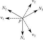
Figure 4.1. The unit vector fields $N_{i}$, $\nu_{i}$ ($i=1,2,3)$ at $p\in S$. $S$ is the spine of the triple junction. $N_{i}$ is normal to $M_{i}$ and $\nu_{i}\in TM_{i}$ is normal to $T_{p}S$ (cf. Figure 1.2, triple junction on the left). The plane of the sheet is perpendicular to the tangent vector $\tau(p)\in T_{p}S$ (not shown).

For the first variation field $w$ we use the following notation:

(4.43) $$\left.\begin{array}[]{l}f_{i}=v_{i}\cdot N_{i}=w\cdot N_{i}\\ h_{i}=u_{i}\cdot\nu_{i}=w\cdot\nu_{i}\\ g_{i}=u_{i}\cdot\tau_{i}=w\cdot\tau_{i}\end{array}\right\}\quad i=1,2,3$$

where $\tau$ is the unit tangent field of the spine such that at any point $p\in S$ the triple $(\tau,\nu_{i},N_{i})$ is positively oriented for all $i=1,2,3$. By (4.42) we have

(4.44) $$\begin{array}[]{l}f_{1}+f_{2}+f_{3}=0\\ h_{1}+h_{2}+h_{3}=0\\ g_{1}=g_{2}=g_{3}=g\end{array}$$

From Figure 4.1 we obtain the following elementary geometric relations:

(4.45) $$\begin{array}[]{l}N_{2}=-\frac{1}{2}N_{1}-\frac{\sqrt{3}}{2}\nu_{1}\\ \nu_{2}=+\frac{\sqrt{3}}{2}N_{1}-\frac{1}{2}\nu_{1}\\ N_{3}=-\frac{1}{2}N_{1}+\frac{\sqrt{3}}{2}\nu_{1}\\ \nu_{3}=-\frac{\sqrt{3}}{2}N_{1}-\frac{1}{2}\nu_{1}\end{array}$$

From these relations and (4.43) we obtain

(4.46) $$\begin{array}[]{l}f_{2}=-\frac{1}{2}f_{1}-\frac{\sqrt{3}}{2}h_{1}\\ h_{2}=+\frac{\sqrt{3}}{2}f_{1}-\frac{1}{2}h_{1}\\ f_{3}=-\frac{1}{2}f_{1}+\frac{\sqrt{3}}{2}h_{1}\\ h_{3}=-\frac{\sqrt{3}}{2}f_{1}-\frac{1}{2}h_{1}\end{array}$$

Equations (4.45), (4.46) express the matching conditions on the spine. When $\gamma_{1}\neq\gamma_{2}\neq\gamma_{3}\neq\gamma_{1}$ we have again linear dependences similar to (4.45), (4.46), with coefficients depending on $\gamma_{1},\gamma_{2},\gamma_{3}$.

Corollary 15.

In the setting of Theorem 12 and assuming that $\gamma_{1}=\gamma_{2}=\gamma_{3}=1$, the expression for the second variation of area (4.34) reduces to

(4.47) $$\begin{gathered}\delta^{2}A^{\star}(T)=\sum_{p,j}\int_{M_{pj}}\left(|\mathrm{grad}_{M_{pj}}f_{pj}|^{2}-|B_{M_{pj}}|^{2}f_{pj}^{2}\right)\\ -\sum_{j=1}^{r}\sum_{p=1}^{3}\int_{\partial M_{pj}\cap\varSigma}f_{pj}^{2}II_{\varSigma}(N_{pj},N_{pj})\\ +\sum_{j=1}^{r}\int_{S_{j}}\left[\alpha_{j}\left(f_{1j}^{2}-h_{1j}^{2}\right)+2\beta_{j}f_{1j}h_{1j}\right]\end{gathered}$$

The $\alpha_{j}$, $\beta_{j}$ are given by

(4.48) $$\alpha_{j}=\frac{\sqrt{3}}{4}\left[II_{M_{2j}}(\nu,\nu)-II_{M_{3j}}(\nu,\nu)\right],\quad\beta_{j}=\frac{3}{4}II_{M_{1j}}(\nu,\nu)$$

The fields $\nu$ correspond to the interface of the indicated second fundamental form.

Remark 16.

Equation (4.47) can be based on phase 2 or 3 instead of phase 1. In this case equations (4.48) must be properly modified. The utility of this expression lies in the independence of the involved variation components.

Proof.

For brevity we write $II_{pj}$ in place of $II_{M_{pj}}(\nu_{pj},\nu_{pj})$. Considering a particular triple junction $T_{j}$, and dropping the corresponding index, i.e. we write $II_{p}$ for $II_{pj}$ and $f_{p}$ for $f_{pj}$, we calculate the sums $\sum_{p}f_{pj}h_{pj}II_{M_{pj}}(\nu,\nu)$ on the third row of (4.34). By the matching conditions (4.46) on the spine we have

$$\sum_{i=1}^{3}f_{i}h_{i}II_{i} =II_{1}f_{1}+II_{2}\left(-\tfrac{1}{2}f_{1}+\tfrac{\sqrt{3}}{2}h_{1}\right)\left(-\tfrac{\sqrt{3}}{2}f_{1}-\tfrac{1}{2}h_{1}\right)$$

$$+II_{3}\left(-\tfrac{1}{2}f_{1}-\tfrac{\sqrt{3}}{2}h_{1}\right)\left(\tfrac{\sqrt{3}}{2}f_{1}-\tfrac{1}{2}h_{1}\right)$$

and performing operations we obtain

$$\sum_{i=1}^{3}f_{i}h_{i}II_{i}=\tfrac{\sqrt{3}}{4}(II_{2}-II_{3})(f_{1}^{2}-h_{1}^{2})+\left(II_{1}-\tfrac{1}{2}II_{2}-\tfrac{1}{2}II_{3}\right)f_{1}h_{1}$$

Setting $\alpha=\frac{\sqrt{3}}{4}(II_{2}-II_{3})$, $\beta=\frac{1}{4}\left(2II_{1}-II_{2}-II_{3}\right)$, and summing over all triple junctions in the system we obtain (4.47). There remains to be proved the second of (4.48).

By the definition of mean curvature vector (2.1), we have on each leaf

$$H\cdot N=\left\langle D_{\nu}\nu,N\right\rangle+\left\langle D_{\tau}\tau,N\right\rangle$$

By minimality $H\cdot N=\kappa=\textrm{const.}$, hence

$$II(\nu,\nu)=\left\langle D_{\nu}\nu,N\right\rangle=\kappa-\left\langle D_{\tau}\tau,N\right\rangle.$$

Summation over the leaves of a triple junction, in view of (3.13) and (4.41), gives

(4.49) $$II_{1}+II_{2}+II_{3}=0.$$

Using this equality in $\beta=\frac{1}{4}\left(2II_{1}-II_{2}-II_{3}\right)$ proves the second of (4.48), and with this the proof is complete. ∎

5. Application to Triple Junction Partitioning Problems in $\mathbb{R}^{3}$

We apply the formula of second variation of area to prove the instability of certain disconnected three-phase triple junction partitioning problems, and demonstrate that the method used for treating disconnectedness in two-phase partitionings has limited applicability to triple junction partitioning problems.

Following the method of two-phase partitioning [13, 14], we consider variations with constant normal component on each leaf. Variations normal to all leaves of a triple junction, other than the trivial, are not possible, for in that case the variation field $w$ would be normal to three linearly independent vectors, viz. $\tau$, the tangent of the spine, and the two tangent fields $\nu_{1}$, $\nu_{2}$ which are normal to the spine. Thus, non-trivial tangential variations $u$ are inevitable, at least in a neighborhood of each spine. For simplicity we take $\gamma_{1}=\gamma_{2}=\gamma_{3}=1$. We dropped the second index on the $\gamma$’s, as they do not depend on the spine (see (3.10)). Since the variation must preserve the volume of the phases, for the triple junction system of Figure 3.1 we have by (3.4) with $w\cdot N=v\cdot N=f$ on each leaf,

(5.1) $$f_{1}A_{1}-f_{31}A_{31}-f_{32}A_{32}=0$$

(5.2) $$-f_{1}A_{1}+f_{21}A_{21}+f_{22}A_{22}=0$$

where $A_{pj}=|M_{pj}|>0$. By (4.46) we obtain

(5.3) $$A_{21}\tilde{h}_{1}+A_{22}\tilde{h}_{2}=\tfrac{1}{\sqrt{3}}\left(2A_{1}+A_{21}+A_{22}\right)\tilde{f}$$

(5.4) $$A_{31}\tilde{h}_{1}+A_{32}\tilde{h}_{2}=-\tfrac{1}{\sqrt{3}}\left(2A_{1}+A_{31}+A_{32}\right)\tilde{f}.$$

where $\tilde{h}_{j}=h_{1j}$ and $\tilde{f}=f_{1}$. Thus the last term of (4.47), on setting $\tilde{f}=1$, becomes

$$\left(1-\tilde{h}_{1}^{2}\right)\int_{S_{1}}\alpha+2\tilde{h}_{1}\int_{S_{1}}\beta+\left(1-\tilde{h}_{2}^{2}\right)\int_{S_{2}}\alpha+2\tilde{h}_{2}\int_{S_{2}}\beta$$

For a stable partition, $\delta^{2}A^{\star}(T)>0$ for nontrivial variations. For constant variations this condition is

$$\begin{split}\left(1-\tilde{h}_{1}^{2}\right)\int_{S_{1}}\alpha+2\tilde{h}_{1}\int_{S_{1}}\beta+\left(1-\tilde{h}_{2}^{2}\right)\int_{S_{2}}\alpha+2\tilde{h}_{2}\int_{S_{2}}\beta>\\ \sum_{p,j}f_{pj}^{2}\int_{M_{pj}}|B_{M_{pj}}|^{2}+\sum_{p,j}f_{pj}^{2}\int_{\partial M_{pj}\cap\varSigma}II_{\varSigma}(N_{pj},N_{pj})\end{split}$$

For convex $\Omega$ the expression on the right side is non-negative, and if we prove that the expression on the left side is non-positive, i.e.

$$\left(1-\tilde{h}_{1}^{2}\right)\int_{S_{1}}\alpha+2\tilde{h}_{1}\int_{S_{1}}\beta+\left(1-\tilde{h}_{2}^{2}\right)\int_{S_{2}}\alpha+2\tilde{h}_{2}\int_{S_{2}}\beta\leqslant 0$$

we get a contradiction, and this would prove that the partitioning is not stable. From what we show in the sequel (see Section 7) it turns out that this condition does not hold in general, and thus the methods of two-phase partitioning are in general not applicable to triple junction partitioning problems.

However, this method can be used to prove instability in certain cases. For example, in the disconnected partitioning of Figure 3.1, assuming that $M_{1}$ is flat, i.e. $II_{1}=0$, we have $\beta=0$. Further, we assume $A_{21}=A_{22}$, $A_{31}=A_{32}$ and $II_{2}\geqslant 0$ for both spines. In this case the system (5.3)-(5.4) has no solution, except when $f_{1}=0$, $\tilde{h}_{2}=-\tilde{h}_{1}$, and then the above condition reduces to

$$-\tilde{h}_{1}^{2}\int_{S_{1}}\alpha-\tilde{h}_{2}^{2}\int_{S_{2}}\alpha\leqslant 0$$

which is true by the hypothesis $II_{2}\geqslant 0$. We have proved the following Proposition.

Proposition 17.

Let $\Omega$ be a convex domain in $\mathbb{R}^{3}$ and $T=(T_{j})_{j=1}^{2}$, $T_{j}=(M_{pj})_{p=1}^{3}$, a minimal disconnected three-phase partition of $\Omega$ by a system of two $C^{2}$ triple junctions as in Figure 3.1, with volume constraints. We assume that $\Sigma=\partial\Omega$ is $C^{2}$ in a neighborhood of $\Sigma\cap\overline{T}$. Further we assume that $M_{1}$ is flat, the areas of the leaves $A_{pj}=|M_{pj}|$ satisfy the condition

$$\left|\begin{array}[]{cc}A_{21}&A_{22}\\ A_{31}&A_{32}\end{array}\right|=0$$

and $II_{2j}(\nu,\nu)\geqslant 0$ for both spines $j=1,2$. Then the disconnected triple junction partition $T$ is unstable.

6. Spectral Analysis of the 2nd Variation Form

To keep the length of formulas to a minimum and focus on the essence of the argument, we present the details for the configuration of Figure 3.1, and adopt the assumption $\gamma_{1}=\gamma_{2}=\gamma_{3}=1$ from this point on.

Let $T$ be a system of triple junctions of a three phase partitioning problem in $\Omega$, which is assumed minimal, i.e. $\delta A(T)=0$. When $T$ is stable, it is a local minimizer of the area functional, so we aim at studying the conditions under which $T$ is stable. To this purpose we will use a spectral analysis method for the bilinear form expressing the second variation of area of $T$,

(6.1) $$\begin{gathered}J(\mathbf{f})=\sum_{p,j}\int_{M_{pj}}\left(|\nabla^{M_{pj}}f_{pj}|^{2}-|B_{M_{pj}}|^{2}f_{pj}^{2}\right)-\sum_{p,j}\int_{\partial M_{pj}\cap\varSigma}\sigma_{pj}f_{pj}^{2}\\ +\sum_{j}\int_{S_{j}}\left[\alpha_{j}\left(f_{1j}^{2}-h_{1j}^{2}\right)+2\beta_{j}f_{1j}h_{1j}\right]\end{gathered}$$

where $\sigma_{pj}=II_{\varSigma}(N_{pj},N_{pj})$ and $\mathbf{f}=(f_{1},f_{21},f_{31},f_{22},f_{32})$. As $f_{11}\equiv f_{12}$ we write simply $f_{1}$. For brevity we will write $\nabla^{M}f$ in place of $\mathrm{grad}_{M}\,f$. Although $J$ and $\delta^{2}A^{\star}(T)$ are identical expressions, their meaning is different: in the context of spectral analysis $T$ is a fixed system of manifolds with boundary and $J$ is a nonlinear functional on a properly defined functional space on $T$ containing the admissible variations of $T$. As a consequence the functions of this space satisfy the conditions of volume constancy

(6.2) $$\begin{cases}-\int_{M_{1}}f_{1}+\int_{M_{21}}f_{21}+\int_{M_{22}}f_{22}=0\\ -\int_{M_{1}}f_{1}+\int_{M_{31}}f_{31}+\int_{M_{32}}f_{32}=0\end{cases}$$

and the normalization condition

(6.3) $$\sum_{p,j}\int_{M_{pj}}f_{pj}^{2}=\int_{M_{1}}f_{1}^{2}+\int_{M_{21}}f_{21}^{2}+\int_{M_{31}}f_{31}^{2}+\int_{M_{22}}f_{22}^{2}+\int_{M_{32}}f_{32}^{2}=1$$

in addition to the compatibility conditions on the spines (see first of (4.44)),

(6.4) $$\begin{cases}f_{1}+f_{21}+f_{31}=0&\textrm{on }S_{1}\\ f_{1}+f_{22}+f_{32}=0&\textrm{on }S_{2}\end{cases}$$

For convenience, we introduce Lagrange multipliers $\lambda_{2},\lambda_{3}$, and the corresponding functional

(6.5) $$\begin{gathered}J^{\star}(\mathbf{f};\mu,\lambda_{2},\lambda_{3})=J(\mathbf{f})-\mu\left(\sum_{p,j}\int_{M_{pj}}f_{pj}^{2}-1\right)\\ -\lambda_{2}\left(-\int_{M_{1}}f_{1}+\int_{M_{21}}f_{21}+\int_{M_{22}}f_{22}\right)\\ -\lambda_{3}\left(-\int_{M_{1}}f_{1}+\int_{M_{31}}f_{31}+\int_{M_{32}}f_{32}\right)\end{gathered}$$

and we are interested in the critical points of $J^{\star}$.

Proposition 18.

A necessary and sufficient condition for a $C^{2}$ function $\mathbf{f}=(f_{1},f_{21},f_{31},f_{22},f_{32})$ on $T$, which satisfies the compatibility conditions (6.4) on the spines, to be a critical point of $J^{\star}$, or equivalently of $J$ with the conditions (6.2) and (6.3), is that it satisfies the following linear inhomogeneous system of PDE

(6.6) $$\Delta_{M_{pj}}f_{pj}+\left(\mu+|B_{M_{pj}}|^{2}\right)f_{pj}=-\tfrac{1}{2}\lambda_{pj}$$

with Neumann-type boundary conditions:

(6.7) $$D_{\nu_{pj}}f_{pj}=\sigma_{pj}f_{pj}\quad\textrm{on}\,\partial M_{pj}\cap\Sigma$$

(6.8) $$\alpha_{j}f_{1j}+\beta_{j}h_{1j}=-D_{\nu_{1j}}f_{1j}+\tfrac{1}{2}\left(D_{\nu_{2j}}f_{2j}+D_{\nu_{3j}}f_{3j}\right)$$

(6.9) $$\beta_{j}f_{1j}-\alpha_{j}h_{1j}=-\tfrac{\sqrt{3}}{2}\left(D_{\nu_{2j}}f_{2j}-D_{\nu_{3j}}f_{3j}\right)$$

Remark 19.

In (6.6) $\Delta_{M}$ is the Laplace-Beltrami operator on $M$ defined by

$$\Delta_{M}f=\mathrm{div}_{M}(\nabla^{M}f)=g^{-1/2}(g^{1/2}g^{ij}f_{,j})_{,i}$$

in a local coordinate system $q^{1},\cdots,q^{n-1}$, where $g=\det\left[g_{ij}\right]$, $g_{ij}$ is the metric tensor and the comma operator denotes partial derivative in the respective coordinate, i.e. $f_{,i}=\frac{\partial f}{\partial q^{i}}=D_{E_{i}}f$. As $M$ is fixed, $g_{ij}$ is fixed and (6.6) is a linear equation.

Remark 20.

The PDE’s (6.6) and the boundary conditions (6.7) are independent of the particular problem, provided that the $\lambda$’s have been defined properly. The boundary conditions (6.8) and (6.9), as well as the definition of the $\lambda$’s are problem specific. For the problem at hand the particular form of the PDE’s is

(6.10) $$\begin{cases}\Delta_{M_{21}}f_{21}+\left(\mu+|B_{M_{21}}|^{2}\right)f_{21}=-\tfrac{1}{2}\lambda_{2}\\ \Delta_{M_{21}}f_{21}+\left(\mu+|B_{M_{21}}|^{2}\right)f_{21}=-\tfrac{1}{2}\lambda_{2}\\ \Delta_{M_{22}}f_{22}+\left(\mu+|B_{M_{22}}|^{2}\right)f_{22}=-\tfrac{1}{2}\lambda_{3}\\ \Delta_{M_{22}}f_{22}+\left(\mu+|B_{M_{22}}|^{2}\right)f_{22}=-\tfrac{1}{2}\lambda_{3}\\ \Delta_{M_{1}}f_{1}+\left(\mu+|B_{M_{1}}|^{2}\right)f_{1}=\tfrac{1}{2}(\lambda_{2}+\lambda_{3})\end{cases}$$

Proof.

The first variation of $J^{\star}$ is given by

$$\delta J^{\star}(\mathbf{f})\boldsymbol{\phi} =\left.\frac{d}{dt}J^{\star}(\mathbf{f}+t\boldsymbol{\phi})\right|_{t=0}$$

$$=2\sum_{p,j}\int_{M_{pj}}\left(\nabla^{M_{pj}}f_{pj}\cdot\nabla^{M_{pj}}\phi_{pj}-|B_{M_{pj}}|^{2}f_{pj}\phi_{pj}\right)$$

$$-2\sum_{p,j}\int_{\partial M_{pj}}\sigma_{pj}f_{pj}\phi_{pj}-2\mu\sum_{p,j}\int_{M_{pj}}f_{pj}\phi_{pj}$$

$$+2\sum_{j}\int_{S_{j}}\left[\alpha_{j}\left(f_{1j}\phi_{1j}-h_{1j}\psi_{1j}\right)+\beta_{j}\left(\phi_{1j}h_{1j}+f_{1j}\psi_{1j}\right)\right]$$

$$-\lambda_{2}\left(-\int_{M_{1}}\phi_{1}+\int_{M_{21}}\phi_{21}+\int_{M_{22}}\phi_{22}\right)$$

$$-\lambda_{3}\left(-\int_{M_{1}}\phi_{1}+\int_{M_{31}}\phi_{31}+\int_{M_{32}}\phi_{32}\right)$$

with

$$\psi_{1j}=\delta h_{1j}=\delta\left[\tfrac{1}{\sqrt{3}}\left(f_{1j}+2f_{2j}\right)\right]=\tfrac{1}{\sqrt{3}}\left(\phi_{1j}+2\phi_{2j}\right)$$

The second equality is obtained by the first of (4.46). By Green’s formula for manifolds, the term on the second row is written in the form

$$-2\sum_{p,j}\int_{M_{pj}}\phi_{pj}\left(\Delta_{M_{pj}}f_{pj}+|B_{M_{pj}}|^{2}f_{pj}\right)+2\sum_{p,j}\int_{\partial M_{pj}}\phi_{pj}D_{\nu_{pj}}f_{pj}$$

and splitting the integrals over $\partial M_{pj}$ into boundary and spine parts

$$\int_{\partial M_{pj}}\phi_{pj}D_{\nu_{pj}}f_{pj}=\int_{\partial M_{pj}\cap\Sigma}\phi_{pj}D_{\nu_{pj}}f_{pj}+\int_{S_{j}}\phi_{pj}D_{\nu_{pj}}f_{pj}$$

we obtain

$$\delta J^{\star}(\mathbf{f})\boldsymbol{\phi} =-2\sum_{p,j}\int_{M_{pj}}\phi_{pj}\left[\Delta_{M_{pj}}f_{pj}+\left(\mu+|B_{M_{pj}}|^{2}\right)f_{pj}\right]$$

$$+2\sum_{p,j}\int_{\partial M_{pj}\cap\Sigma}\phi_{pj}\left(D_{\nu_{pj}}f_{pj}-\sigma_{pj}f_{pj}\right)$$

$$+2\sum_{p,j}\int_{S_{j}}\phi_{pj}D_{\nu_{pj}}f_{pj}$$

$$+2\sum_{j}\int_{S_{j}}\left[\alpha_{j}\left(f_{1j}\phi_{1j}-h_{1j}\psi_{1j}\right)+\beta_{j}\left(\phi_{1j}h_{1j}+f_{1j}\psi_{1j}\right)\right]$$

$$-\sum_{p,j}\lambda_{pj}\int_{M_{pj}}\phi_{pj}$$

We have set $\lambda_{11}=-(\lambda_{2}+\lambda_{3})$, $\lambda_{21}=\lambda_{22}=\lambda_{2}$ and $\lambda_{31}=\lambda_{32}=\lambda_{3}$. Using compactly supported variations vanishing on all $\partial M_{pj}\cap\Sigma$ and $S_{j}$ we obtain (6.6). Variations $\boldsymbol{\phi}$ concentrated on $\partial M_{pj}\cap\Sigma$ give (6.7). The remaining terms are integrals over spines:

$$\delta J^{\star}(\mathbf{f})\boldsymbol{\phi} =2\sum_{p,j}\int_{S_{j}}\phi_{pj}D_{\nu_{pj}}f_{pj}$$

$$+2\sum_{j}\int_{S_{j}}\left[\alpha_{j}\left(f_{1j}\phi_{1j}-h_{1j}\psi_{1j}\right)+\beta_{j}\left(\phi_{1j}h_{1j}+f_{1j}\psi_{1j}\right)\right]$$

Using the identities (4.44) to express the $\phi_{3j}$ in terms of independent quantities,

$$\phi_{3j}=\delta f_{3j}=-\delta f_{1j}-\delta f_{2j}=-\phi_{1j}-\phi_{2j},$$

expanding out and collecting similar terms,

$$\delta J^{\star}(\mathbf{f}) =2\sum_{j}\int_{S_{j}}\phi_{1j}D_{\nu_{1j}}f_{1j}+\phi_{2j}D_{\nu_{2j}}f_{2j}+\phi_{3j}D_{\nu_{3j}}f_{3j}$$

$$+2\sum_{j}\int_{S_{j}}\left[\alpha_{j}\left(f_{1j}\phi_{1j}-h_{1j}\psi_{1j}\right)+\beta_{j}\left(\phi_{1j}h_{1j}+f_{1j}\psi_{1j}\right)\right]$$

$$=2\sum_{j}\int_{S_{j}}\phi_{1j}\left(D_{\nu_{1j}}f_{1j}-D_{\nu_{3j}}f_{3j}\right)+\phi_{2j}\left(D_{\nu_{2j}}f_{2j}-D_{\nu_{3j}}f_{3j}\right)$$

$$+2\sum_{j}\int_{S_{j}}\phi_{1j}\left(\alpha_{j}f_{1j}+\beta_{j}h_{1j}\right)+2\sum_{j}\int_{S_{j}}\psi_{1j}\left(\beta_{j}f_{1j}-\alpha_{j}h_{1j}\right)$$

Substituting for $\phi_{2j}$ by $\phi_{2j}=\frac{\sqrt{3}}{2}\psi_{1j}-\frac{1}{2}\phi_{1j}$, and performing operations gives

$$\delta J^{\star}(\mathbf{f}) =2\sum_{j}\int_{S_{j}}\phi_{1j}\left[D_{\nu_{1j}}f_{1j}-\tfrac{1}{2}D_{\nu_{2j}}f_{2j}-\tfrac{1}{2}D_{\nu_{3j}}f_{3j}+\alpha_{j}f_{1j}+\beta_{j}h_{1j}\right]$$

$$+2\sum_{j}\int_{S_{j}}\psi_{1j}\left(\tfrac{2}{\sqrt{3}}D_{\nu_{2j}}f_{2j}-\tfrac{2}{\sqrt{3}}D_{\nu_{3j}}f_{3j}+\beta_{j}f_{1j}-\alpha_{j}h_{1j}\right)$$

Using variations concentrated on each spine we obtain (6.8) and (6.9). The converse is immediate. ∎

In the following we present two propositions that are necessary for the study of stability of triple junction partitionings. The next proposition states that a partitioning problem is unstable if there is an eigenvalue $\mu<0$ of the system (6.6)-(6.9).

Proposition 21.

Let $T$ be a system of $C^{2}$ triple junctions of a minimal three phase partitioning problem in $\Omega$, and $\mathbf{f}$ an eigenfunction of problem (6.6)-(6.9) with corresponding eigenvalue $\mu$. Then

(6.11) $$J(\mathbf{f})=\mu.$$

In particular, if $\mu<0$, $T$ is unstable.

Remark 22.

Proposition 21 implies that, with a negative eigenvalue at hand, no lower bound is needed to be known in advance for the functional $J$, in order to conclude that a minimal partitioning is unstable.

Proof.

Multiplication of (6.6) by $f_{pj}$, integration over $M_{pj}$ and summation over all leaves of all triple junctions, gives in view of (6.2) and (6.3)

$$\sum_{p,j}\int_{M_{pj}}\left(f_{pj}\Delta_{M_{pj}}f_{pj}+|B_{M_{pj}}|^{2}f_{pj}^{2}\right)+\mu=0$$

Application of Green’s formula gives

$$\sum_{p,j}\int_{M_{pj}}\left(|\nabla^{M_{pj}}f_{pj}|^{2}-|B_{M_{pj}}|^{2}f_{pj}^{2}\right)-\sum_{p,j}\int_{\partial M_{pj}}f_{pj}D_{\nu_{pj}}f_{pj}=\mu$$

On breaking the integrals over $\partial M_{pj}$ into boundary and spine parts and using the boundary condition (6.7), we obtain

$$\begin{gathered}\sum_{p,j}\int_{M_{pj}}\left(|\nabla^{M_{pj}}f_{pj}|^{2}-|B_{M_{pj}}|^{2}f_{pj}^{2}\right)-\sum_{p,j}\int_{\partial M_{pj}\cap\Sigma}\sigma_{pj}f_{pj}^{2}\\ -\sum_{p,j}\int_{S_{j}}f_{pj}D_{\nu_{pj}}f_{pj}=\mu\end{gathered}$$

Furthermore, on each spine we have

$$\begin{gathered}\alpha_{j}\left(f_{1j}^{2}-h_{1j}^{2}\right)+2\beta_{j}f_{1j}h_{1j}=f_{1j}(\alpha_{j}f_{1j}+\beta_{j}h_{1j})+h_{1j}(\beta_{j}f_{1j}-\alpha_{j}h_{1j})=\\ f_{1j}\left[-D_{\nu_{1j}}f_{1j}+\tfrac{1}{2}\left(D_{\nu_{2j}}f_{2j}+D_{\nu_{3j}}f_{3j}\right)\right]-\tfrac{\sqrt{3}}{2}h_{1j}\left(D_{\nu_{2j}}f_{2j}-D_{\nu_{3j}}f_{3j}\right)=\\ \sum_{p}f_{pj}D_{\nu_{pj}}f_{pj}\end{gathered}$$

after using (4.46) and performing straight-forward operations. By the definition of $J$ (6.1) we obtain $J(\mathbf{f})=\mu$. The second assertion follows immediately from this. ∎

Proposition 21 can be used to prove instability. The method we follow to establish the stability of a specific partitioning problem, is to prove that the minimal eigenvalue of $J$, or equivalently of the boundary value problem (6.6)-(6.9), is positive. We provide a justification of this method. The difficulty is that the boundary integral $\int_{\partial M}f^{2}$ cannot be bounded above by $\int_{M}f^{2}$. However, if $f\in W^{1,2}(M)\equiv H^{1}(M)$, the boundary trace embedding theorem ([20] §§ 5.34-5.37, pp 163-166; [21] § 8, pp 120-132) and a suitable interpolation estimate (see Lemma 24 below) yield the coercivity of $J$. From this by a well-known theorem (see proof of Proposition 25) we obtain the existence of a minimal eigenvalue for $J$.

The standard notation for Sobolev spaces is used: $|u|_{L^{2}(M)}=(\int_{M}u^{2})^{1/2}$, $|u|_{H^{1}(M)}=(|u|_{L^{2}(M)}^{2}+|\nabla^{M}u|_{L^{2}(M)}^{2})^{1/2}$, $|u|_{L^{2}(\partial M)}=(\int_{\partial M}u^{2})^{1/2}$ are the standard norms of $L^{2}(M)$, $H^{1}(M)$ and $L^{2}(\partial M)$. Let $T$ be a partitioning of $\Omega$ by a system of triple junctions. Sobolev spaces on $T$ are defined as follows:

$$H^{1}(T)=\prod_{j=1}^{r}\prod_{p=1}^{3}H^{1}(M_{pj})$$

It is understood that each distinct $M_{pj}$ participates in the product only once. The $L^{2}$-norm is

$$|\mathbf{f}|_{L^{2}(T)}=\left(\sum_{p,j}|f_{pj}|_{L^{2}(M_{pj})}^{2}\right)^{1/2}$$

and the $H^{1}(T)$-norm is defined analogously. Further, we define the functionals

$$\varphi_{p}(\mathbf{f})=\sum_{j=1}^{r}\sum_{q\neq p}\varepsilon_{pqj}\int_{M_{qj}}f_{qj}\quad(p,q=1,2,3)$$

where

$$\varepsilon_{pqj}=\begin{cases}+1,&N_{qj}\>\textrm{outward}\>\textrm{to}\>\Omega_{pj}\\ -1,&N_{qj}\>\textrm{inward}\>\textrm{to}\>\Omega_{pj}\end{cases}$$

Clearly $\sum_{p}\varphi_{p}(\mathbf{f})=0$ and the volume constraints can be expressed by means of these functionals.

Example 23.

For the triple junction system of Figure 3.1 the $\varphi$-functionals are

$$\varphi_{1}(\mathbf{f})= \int_{M_{21}}f_{21}+\int_{M_{22}}f_{22}-\int_{M_{31}}f_{31}-\int_{M_{32}}f_{32}$$

$$\varphi_{2}(\mathbf{f})= -\int_{M_{1}}f_{1}+\int_{M_{31}}f_{31}+\int_{M_{32}}f_{32}$$

$$\varphi_{3}(\mathbf{f})= -\int_{M_{1}}f_{1}+\int_{M_{21}}f_{21}+\int_{M_{22}}f_{22}$$

The volume constraints are given by $\varphi_{2}(\mathbf{f})=0$, $\varphi_{3}(\mathbf{f})=0$.

The following estimate is easily established for $\mathbf{f}\in L^{2}(T)$:

(6.12) $$|\varphi_{p}(\mathbf{f})|\leqslant c_{0}|\mathbf{f}|_{L^{2}(T)},\quad p=1,2,3.$$

Lemma 24.

Let $M$ be a bounded $C^{2}$ submanifold of $\mathbb{R}^{n}$ with boundary. Then for every $\epsilon>0$ there is a constant $c_{\epsilon}$ such that for any $u\in H^{1}(M)$

(6.13) $$|u|_{L^{2}(\partial M)}\leqslant\epsilon|u|_{H^{1}(M)}+c_{\epsilon}|u|_{L^{2}(M)}$$

For the proof see [14].

After this preparation we can prove the following result, which is the basis of our method for establishing stability.

Proposition 25.

Let $T$ be a minimal three phase partitioning of $\Omega\subset\mathbb{R}^{3}$ by a system of triple junctions. Then for any $\mathbf{f}=(f_{pj})\in H^{1}(T)$ satisfying the compatibility conditions on the spines and (6.2), (6.3) we have

(6.14) $$J(\mathbf{f})\geqslant\mu_{1}$$

where $\mu_{1}$ is the smallest eigenvalue of problem (6.6)-(6.9). In particular, if $\mu_{1}>0$, $T$ is stable.

Proof.

We will prove that the conditions of Theorem 1.2 in [22] are satisfied. Let

$$X=\{u\in H^{1}(T):|u|_{L^{2}(T)}\leqslant 1,\,\sum_{p}u_{pj}=0\,\textrm{on }S_{j},\,\varphi_{2}(u)=\varphi_{3}(u)=0\}.$$

By the continuity of the $L^{2}(T)$-norm, the functionals $\varphi_{p}:H^{1}(T)\to\mathbb{R}$, and the mappings $u\mapsto\left.\sum_{p}u_{pj}\right|_{S_{j}}$, it follows that $X$ is a closed subset of $H^{1}(T)$. The convexity of $X$ is clear. Hence $X$ is a weakly closed subset of $H^{1}(T)$. We prove the coercivity of $J$ on $X$. By continuity there are non-negative constants $\sigma_{0}$, $b_{0}$, $\alpha_{0}$ such that

$$\sigma_{pj}\leqslant\sigma_{0},\;|B_{M_{pj}}|^{2}\leqslant b_{0},\;|\alpha_{j}|\leqslant\tfrac{1}{2}\alpha_{0},\;|\beta_{j}|\leqslant\tfrac{1}{2}\alpha_{0}$$

for all $p,j$. By the inequalities

$$\alpha_{j}\left(f_{1j}^{2}-h_{1j}^{2}\right)\geqslant-\tfrac{1}{2}\alpha_{0}\left(f_{1j}^{2}+h_{1j}^{2}\right),\quad 2\beta_{j}f_{1j}h_{1j}\geqslant-\alpha_{0}|f_{1j}h_{1j}|$$

which are easily established, we obtain

$$\alpha_{j}\left(f_{1j}^{2}-h_{1j}^{2}\right)+2\beta_{j}f_{1j}h_{1j}\geqslant-\alpha_{0}\left(f_{1j}^{2}+h_{1j}^{2}\right)$$

and using the first of (4.46),

$$\alpha_{j}\left(f_{1j}^{2}-h_{1j}^{2}\right)+2\beta_{j}f_{1j}h_{1j}\geqslant-2\alpha_{0}\left(f_{1j}^{2}+f_{2j}^{2}\right)$$

Thus by (6.1), with possibly redefined values of $b_{0}$, $\sigma_{0}$, we obtain the estimate

$$J(\mathbf{f})\geqslant\sum_{p,j}|f_{pj}|_{H^{1}(M_{pj})}^{2}-b_{0}\sum_{p,j}|f_{pj}|_{L^{2}(M_{pj})}^{2}-\sigma_{0}\sum_{p,j}\int|f_{pj}|_{L^{2}(\partial M_{pj})}^{2}$$

By the interpolation inequality (6.13),

$$J(\mathbf{f})\geqslant(1-\epsilon\sigma_{0})\sum_{p,j}|f_{pj}|_{H^{1}(M_{pj})}^{2}-(b_{0}+c_{\epsilon}\sigma_{0})\sum_{p,j}|f_{pj}|_{L^{2}(M_{pj})}^{2}$$

which for sufficiently small value of $\epsilon>0$ proves the coercivity of $J$. The sequential weakly lower semicontinuity of $J$ follows from the sequential weakly lower semicontinuity of the norm of $H^{1}(T)$ and the compactness of the embedding $H^{1}(M)\hookrightarrow L^{2}(M)$. Thus the conditions of Theorem 1.2 in [22] are satisfied, and from this we conclude that $J$ attains its infimum in $X$. The position of the infimum is a critical point of $J^{\star}$ and, as it was shown in Proposition 21, it is a solution of equation (6.6) with BC (6.7). The inequality (6.14) follows immediately form this. ∎

7. Application to Disconnected 2-Dimensional Partitioning Problems

We prove the existence of stable disconnected partitionings in 2 dimensions by example.

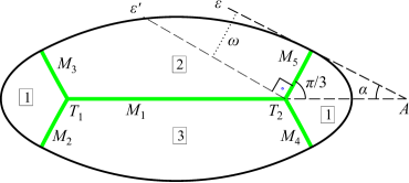
Figure 7.1. Disconnected three phase partitioning consisting of two triple junctions. Boxed numbers indicate phases. $T_{1}$ and $T_{2}$ are the triple junctions. The leaves of the triple junctions $M_{2},\cdots,M_{5}$ are circular arcs of the same curvature $\kappa$ (absolute value) while $M_{1}$ is flat. By minimality the tangent to $M_{5}$ at $T_{2}$ is at angle $\pi/3$ with the line $T_{1}A$. $A\varepsilon$ is the tangent to $\Sigma=\partial\Omega$ at $M_{5}\cap\Sigma$ and $T_{2}\varepsilon^{\prime}$ is the normal to the tangent of $M_{5}$ at $T_{2}$. The intersection $C$ (not shown in the Figure) of $A\varepsilon$ and $T_{2}\varepsilon^{\prime}$ is the center of the circle with radius $R=1/\kappa$ containing the circular arc $M_{5}$. Since $\omega=\widehat{ACT}_{2}$, by plane geometry, $\omega=\frac{\pi}{6}-\alpha$. Analogous relations hold for the other leaves. This Figure was produced by an Octave (MATLAB) program. The boundary $\Sigma$ was drawn as a set of four four-degree splines having curvature zero at their ends $M_{i}\cap\Sigma$, $i=2,\cdots,5$. The indicated boundary is symmetric about the $x$ and $y$ axes, but a non-symmetric boundary could also be drawn for the same triple junction arrangement.

For two-dimensional partitions the Laplace-Beltrami operator reduces to

$$\Delta_{M}f=\frac{d^{2}f}{ds^{2}}$$

where $s$ is the arc length of $M$, $M$ being any triple junction leaf, and the integrals over $\partial M$ reduce to numbers. The boundary condition (6.7) reduces to

(7.1) $$\frac{df}{ds}=0,\;\textrm{on}\,\partial M\cap\Sigma$$

As we are interested in proving the existence of stable disconnected partitionings, we have chosen $\sigma=0$ at $\partial M\cap\Sigma$. From part (ii) of Proposition 7 the curvature of each leaf is constant, thus the only possibilities for $M$ are line segments and circular arcs. Further, $|B_{M}|=\kappa=1/R$, where $R$ is the radius of the arc or $\infty$ for line segments. We consider disconnected partitionings having the topology of Figure 7.1. We are using the sequential enumeration notation of Example 6 in which $\mathbf{f}=(f_{1},\cdots,f_{5})$, $T=(M_{1},\cdots,M_{5})$.

For equation (6.6) we have the following three types of solution, depending on the sign of $\mu+|B_{M}|^{2}$,

$$(I) \quad f(s)=-\frac{\lambda}{2k^{2}}+C\sin(ks)+D\cos(ks), k^{2}=\mu+\kappa^{2}\Leftrightarrow\mu>-\kappa^{2}$$

$$(II) \quad f(s)=\frac{\lambda}{2k^{2}}+Ce^{ks}+De^{-ks}, k^{2}=-(\mu+\kappa^{2})\Leftrightarrow\mu<-\kappa^{2}$$

$$(III) \quad f(s)=-\frac{\lambda}{4}s^{2}+Cs+D, \mu=-\kappa^{2}$$

and

$$\lambda_{1}=-(\lambda_{2}+\lambda_{3}),\;\lambda_{4}=\lambda_{2},\;\lambda_{5}=\lambda_{3}$$

while the $\lambda_{2},\,\lambda_{3}$ are independent variables. The parametrizations of the $M_{i}$ (with the exception of $M_{1}$ which does not intersect $\Sigma$) are such that $M_{i}\cap\Sigma$ is obtained at $s=l_{i}$, where $l_{i}=|M_{i}|$ is the length of $M_{i}$. From the BC (7.1) we obtain for the three cases ($i\neq 1)$

$$(I)\;D_{i}=C_{i}\cot(k_{i}l_{i}),\quad(II)\;D_{i}=C_{i}e^{2k_{i}l_{i}},\quad(III)\;C_{i}=-\tfrac{1}{2}\lambda_{i}l_{i}$$

and

$$(I) \quad f_{i}(s)=-\frac{\lambda_{i}}{2k_{i}^{2}}+\frac{C_{i}}{\sin(k_{i}l_{i})}\cos k_{i}(s-l_{i}),$$

$$(II) \quad f_{i}(s)=\frac{\lambda_{i}}{2k_{i}^{2}}+C_{i}e^{2k_{i}l_{i}}\cosh k_{i}(s-l_{i}),$$

$$(III) \quad f(s)=-\frac{\lambda_{i}}{4}(s-l_{i})^{2}+\frac{\lambda_{i}l_{i}^{2}}{4}+D_{i},$$

Since $f_{1}$ contains 2 constants while all other $f$’s only one, we have in total 6 unknown constants, which together with $\lambda_{2}$, and $\lambda_{3}$ make 8 unknowns. On the other hand, two volume constraints, the BC’s (6.8), (6.9), and the compatibility condition on the two spines (see first of (4.44)) are 8 equations in total, and in this way we have a linear system of 8 equations in 8 unknowns. The condition for existence of solutions of this system is, as usually, obtained by setting its determinant to 0, which gives a nonlinear equation for $k$. With a solution for $k$ at hand, we can determine the eigenvalue $\mu$ by the last column in the above table of possible solutions for $f$, and each eigenvector determines an eigenfunction $f$ of problem (6.6)-(6.9).

We specialize these relations by considering the case of Figure 7.1 in which the leaves $M_{2}$, $M_{3}$, $M_{4}$ and $M_{5}$ have the same radius $R=1/\kappa$ and the same length $l$, while $M_{1}$ is flat and has length $L$. In this case

$$II_{M_{21}}(\nu,\nu)=II_{M_{22}}(\nu,\nu)=-\frac{1}{R}=-\kappa$$

$$II_{M_{31}}(\nu,\nu)=II_{M_{32}}(\nu,\nu)=\kappa,\;II_{M_{1}}(\nu,\nu)=-(II_{M_{21}}+II_{M_{31}})=0$$

and

$$\alpha=-\frac{\sqrt{3}}{2}\kappa<0,\quad\beta=0$$

for both spines.

We distinguish the following cases for $\mu$:

7.1. Case I: $-\kappa^{2}<\mu<0,\;k^{2}=\mu+\kappa^{2}\,(0<\frac{k}{\kappa}<1)$

For $i\neq 1$ we have $\mu+|B_{M_{i}}|^{2}=\mu+\kappa^{2}>0$, and $\mu+|B_{M_{i}}|^{2}=\mu<0$, so we have a solution type (I) on $M_{2}$, $M_{3}$, $M_{4}$, $M_{5}$ and type (II) on $M_{1}$. Thus

(7.2) $$f_{1}(s)=-\frac{\lambda_{2}+\lambda_{3}}{2(\kappa^{2}-k^{2})}+C_{1}e^{\sqrt{\kappa^{2}-k^{2}}s}+D_{1}e^{-\sqrt{\kappa^{2}-k^{2}}s}$$

$$f_{i}(s)=-\frac{\lambda_{i}}{2k^{2}}+\frac{C_{i}}{\sin(kl)}\cos\left[k(s-l)\right],\quad i=2,\cdots,5$$

and their derivatives are given by

$$f_{1}^{\prime}(s)=\sqrt{\kappa^{2}-k^{2}}\left(C_{1}e^{\sqrt{\kappa^{2}-k^{2}}s}-D_{1}e^{-\sqrt{\kappa^{2}-k^{2}}s}\right)$$

$$f_{i}^{\prime}(s)=-\frac{kC_{i}}{\sin(kl)}\sin\left[k(s-l)\right],\quad i=2,\cdots,5$$

In the second of (7.2) it is $\sin(kl)\neq 0$, for otherwise $k=\frac{n\pi}{l}$, $n\in\mathbb{Z}$, and by $0<k<\kappa$ it follows that $0<n<\frac{\kappa l}{\pi}$. However, by simple geometric arguments, $\kappa l=\frac{l}{R}\leqslant\frac{\pi}{3}$.

On spine 1 we have

$$D_{\nu_{1}}f_{1}(0)=-f_{1}^{\prime}(0)=-\sqrt{\kappa^{2}-k^{2}}\left(C_{1}-D_{1}\right)$$

$$D_{\nu_{2}}f_{2}(0)=-f_{2}^{\prime}(0)=-kC_{2}$$

$$D_{\nu_{3}}f_{3}(0)=-f_{3}^{\prime}(0)=-kC_{3}$$

and similarly on spine 2,

$$D_{\nu_{1}}f_{1}(L)=+f_{1}^{\prime}(L)=\sqrt{\kappa^{2}-k^{2}}\left(C_{1}e^{\sqrt{\kappa^{2}-k^{2}}L}-D_{1}e^{-\sqrt{\kappa^{2}-k^{2}}L}\right)$$

$$D_{\nu_{4}}f_{4}(0)=-f_{4}^{\prime}(0)=-kC_{4}$$

$$D_{\nu_{5}}f_{5}(0)=-f_{5}^{\prime}(0)=-kC_{5}$$

For brevity we set

$$\textrm{Case}\,\textrm{I:}\quad a=\frac{2}{\sqrt{3}}\sqrt{1-\left(\frac{k}{\kappa}\right)^{2}},\;z=e^{L\sqrt{\kappa^{2}-k^{2}}},\;b=\frac{2l}{k^{2}}-\frac{L}{\kappa^{2}-k^{2}}$$

From the conditions (6.8), (6.9) on spine 1 we obtain

(7.3) $$\lambda_{2}-\lambda_{3}-2k^{2}\left[\cot(kl)-\frac{\sqrt{3}}{2}\frac{k}{\kappa}\right](C_{2}-C_{3})=0$$

(7.4) $$\frac{\lambda_{2}+\lambda_{3}}{2(\kappa^{2}-k^{2})}-\left(a+1\right)C_{1}+\frac{1}{\sqrt{3}}\frac{k}{\kappa}(C_{2}+C_{3})+\left(a-1\right)D_{1}=0$$

By the compatibility condition $f_{1}+f_{2}+f_{3}=0$ on spine 1 we obtain

(7.5) $$-\frac{1}{2}\left(\frac{1}{\kappa^{2}-k^{2}}+\frac{1}{k^{2}}\right)(\lambda_{2}+\lambda_{3})+C_{1}+(C_{2}+C_{3})\cot(kl)+D_{1}=0$$

From the conditions (6.8), (6.9) on spine 2 we obtain

(7.6) $$\lambda_{2}-\lambda_{3}-2k^{2}\left[\cot(kl)-\frac{\sqrt{3}}{2}\frac{k}{\kappa}\right](C_{4}-C_{5})=0$$

(7.7) $$\frac{\lambda_{2}+\lambda_{3}}{2(\kappa^{2}-k^{2})}+\left(a-1\right)zC_{1}+\frac{1}{\sqrt{3}}\frac{k}{\kappa}(C_{4}+C_{5})-\left(a+1\right)\frac{1}{z}D_{1}=0$$

The equality $f_{1}+f_{2}+f_{3}=0$ on spine 2 gives

(7.8) $$-\frac{1}{2}\left(\frac{1}{\kappa^{2}-k^{2}}+\frac{1}{k^{2}}\right)(\lambda_{2}+\lambda_{3})+zC_{1}+(C_{4}+C_{5})\cot(kl)+\frac{1}{z}D_{1}=0$$

Finally the volume conservation equations (4.37) give the equations

(7.9) $$b\frac{\lambda_{2}}{2}-\frac{L}{\kappa^{2}-k^{2}}\frac{\lambda_{3}}{2}+\frac{z-1}{\sqrt{\kappa^{2}-k^{2}}}\left(C_{1}+\frac{1}{z}D_{1}\right)-\frac{1}{k}(C_{2}+C_{4})=0$$

(7.10) $$-\frac{L}{\kappa^{2}-k^{2}}\frac{\lambda_{2}}{2}+b\frac{\lambda_{3}}{2}+\frac{z-1}{\sqrt{\kappa^{2}-k^{2}}}\left(C_{1}+\frac{1}{z}D_{1}\right)-\frac{1}{k}(C_{3}+C_{5})=0$$

The following lemma allows the reduction of this system to a simpler one.

Lemma 26.

Assume $\left[\tan(\kappa l)+\sqrt{3}\right]\kappa L<4$. Then the $8\times 8$ linear system of equations (7.3)-(7.10) is equivalent to the following $3\times 3$ linear system

$$(S_{1})\;\begin{cases}\frac{1}{\kappa^{2}-k^{2}}\lambda_{2}+\left[(a-1)z-a-1\right]C_{1}+\frac{2}{\sqrt{3}}\frac{k}{\kappa}C_{2}=0\\ \left(\frac{1}{\kappa^{2}-k^{2}}+\frac{1}{k^{2}}\right)\lambda_{2}-(z+1)C_{1}-2C_{2}\cot(kl)=0\\ \left(\frac{l}{k^{2}}-\frac{L}{\kappa^{2}-k^{2}}\right)\lambda_{2}+2\frac{z-1}{\sqrt{\kappa^{2}-k^{2}}}C_{1}-\frac{2}{k}C_{2}=0\end{cases}$$

and $C_{2}=C_{3}=C_{4}=C_{5}$, $D_{1}=zC_{1}$, $\lambda_{2}=\lambda_{3}$.

Remark 27.

The condition is satisfied if $\kappa L<\sqrt{3}$, for by simple geometric arguments (see Figure 7.1) $\kappa l=\omega<\frac{\pi}{6}$, and $\tan(\kappa l)<\frac{1}{\sqrt{3}}$.

Proof.

The pairs of equations (7.9), (7.10) and (7.3), (7.6) give

(7.11) $$C_{2}-C_{3}+C_{4}-C_{5}=\frac{l}{k}(\lambda_{2}-\lambda_{3})$$

and

$$\left[\cot(kl)-\frac{\sqrt{3}}{2}\frac{k}{\kappa}\right](C_{2}-C_{3}-C_{4}+C_{5})=0$$

Since $\cot(kl)\not=\frac{\sqrt{3}}{2}\frac{k}{\kappa}$, which follows from $\frac{\sqrt{3}}{2}\frac{k}{\kappa}\tan(kl)<\frac{\sqrt{3}}{2}\tan\omega<\frac{1}{2}$ and $\omega<\frac{\pi}{6}$ (see Figure 7.1), we obtain

(7.12) $$C_{2}-C_{3}-C_{4}+C_{5}=0$$

By equations (7.5), (7.8) we obtain

(7.13) $$C_{2}+C_{3}-C_{4}-C_{5}=(C_{1}-\frac{1}{z}D_{1})(z-1)\tan(kl)$$

and by (7.4), (7.7)

(7.14) $$C_{2}+C_{3}-C_{4}-C_{5}=\sqrt{3}(C_{1}-\frac{1}{z}D_{1})\frac{\kappa}{k}\left[(a-1)z+a+1\right]$$

The last two equations give

(7.15) $$D_{1}=zC_{1}$$

and

$$\frac{k}{\kappa}\tan(kl)+\sqrt{3}\left(1-a\frac{z+1}{z-1}\right)=0$$

which on setting $x=\frac{k}{\kappa}$, $l^{\star}=\kappa l$, $L^{\star}=\kappa L$ and using the expression of $a$, assumes the form

(7.16) $$x\tan(l^{\star}x)=2\sqrt{1-x^{2}}\frac{z+1}{z-1}-\sqrt{3}.$$

The function on the right side is decreasing and thus attains its minimum at $x=1$, hence it is greater than $\frac{4}{L^{\star}}-\sqrt{3}$. From $x\tan(l^{\star}x)<\tan(l^{\star})=\tan(\kappa l)$ and the hypothesis, it follows that equation (7.16) has no solution.

By (7.14), (7.15) and (7.11), (7.12) we obtain

(7.17) $$C_{2}+C_{3}-C_{4}-C_{5}=0$$

(7.18) $$C_{2}-C_{3}=C_{4}-C_{5}=\frac{l}{2k}(\lambda_{2}-\lambda_{3})$$

By (7.3) and (7.18) it follows that

$$(\lambda_{2}-\lambda_{3})\left[kl\left(\cot(kl)-\frac{\sqrt{3}}{2}\frac{k}{\kappa}\right)-1\right]=0$$

and from this and $\cot(kl)-\frac{\sqrt{3}}{2}\frac{k}{\kappa}<0$, $\lambda_{2}=\lambda_{3}$. Use of equations (7.17), (7.18), and the remaining equations of system (7.3)-(7.10), i.e. (7.4), (7.5) and (7.9), completes the proof. ∎

7.2. Case II: $\mu<-\kappa^{2},\;k>0$

Here $k$ is defined by $k^{2}=-(\mu+\kappa^{2})$, so that the valid range of $k$ is $k>0$. In this case $k_{i}=k$ for $i=2,\cdots,5$ and $k_{1}=-(\mu+\kappa_{1}^{2})=-\mu>0$. Thus we have a solution type (II) for all $f_{i}$,

(7.19) $$f_{1}(s)=-\frac{\lambda_{2}+\lambda_{3}}{2(k^{2}+\kappa^{2})}+C_{1}e^{\sqrt{k^{2}+\kappa^{2}}s}+D_{1}e^{-\sqrt{k^{2}+\kappa^{2}}s}$$

$$f_{i}(s)=\frac{\lambda_{i}}{2k^{2}}+2C_{i}e^{kl}\cosh k(s-l),\quad i=2,\cdots,5$$

and their derivatives are given by

$$f_{1}^{\prime}(s)=\sqrt{k^{2}+\kappa^{2}}\left(C_{1}e^{\sqrt{k^{2}+\kappa^{2}}s}-D_{1}e^{-\sqrt{k^{2}+\kappa^{2}}s}\right)$$

$$f_{i}^{\prime}(s)=2kC_{i}e^{kl}\sinh k(s-l),\quad i=2,\cdots,5$$

Proceeding as in case I we obtain the following linear system:

(7.20) $$\frac{\lambda_{2}-\lambda_{3}}{2k^{2}}+\left[\left(\frac{\sqrt{3}}{2}\frac{k}{\kappa}+1\right)e^{2kl}-\left(\frac{\sqrt{3}}{2}\frac{k}{\kappa}-1\right)\right](C_{2}-C_{3})=0$$

(7.21) $$\frac{\lambda_{2}-\lambda_{3}}{2(k^{2}+\kappa^{2})}-(a+1)C_{1}-\frac{1}{\sqrt{3}}\frac{k}{\kappa}(e^{2kl}-1)(C_{2}+C_{3})+(a-1)D_{1}=0$$

(7.22) $$\frac{\lambda_{2}-\lambda_{3}}{2}\left(\frac{1}{k^{2}}-\frac{1}{k^{2}+\kappa^{2}}\right)+C_{1}+(e^{2kl}+1)(C_{2}+C_{3})+D_{1}=0$$

(7.23) $$\frac{\lambda_{2}+\lambda_{3}}{2k^{2}}+\left[\left(\frac{\sqrt{3}}{2}\frac{k}{\kappa}+1\right)e^{2kl}-\left(\frac{\sqrt{3}}{2}\frac{k}{\kappa}-1\right)\right](C_{4}-C_{5})=0$$

(7.24) $$\frac{\lambda_{2}-\lambda_{3}}{2(k^{2}+\kappa^{2})}+(a-1)zC_{1}-\frac{1}{\sqrt{3}}\frac{k}{\kappa}(e^{2kl}-1)(C_{4}+C_{5})-(a+1)\frac{1}{z}D_{1}=0$$

(7.25) $$\frac{\lambda_{2}+\lambda_{3}}{2}\left(\frac{1}{k^{2}}-\frac{1}{k^{2}+\kappa^{2}}\right)+zC_{1}+(e^{2kl}+1)(C_{4}+C_{5})+\frac{1}{z}D_{1}=0$$

(7.26) $$-b\frac{\lambda_{2}}{2}-\frac{L}{k^{2}+\kappa^{2}}\frac{\lambda_{3}}{2}+\frac{z-1}{\sqrt{k^{2}+\kappa^{2}}}\left(C_{1}+\frac{1}{z}D_{1}\right)-\frac{e^{2kl}-1}{k}(C_{2}+C_{4})=0$$

(7.27) $$-\frac{L}{k^{2}+\kappa^{2}}\frac{\lambda_{2}}{2}-b\frac{\lambda_{3}}{2}+\frac{z-1}{\sqrt{k^{2}+\kappa^{2}}}\left(C_{1}+\frac{1}{z}D_{1}\right)-\frac{e^{2kl}-1}{k}(C_{3}+C_{5})=0$$

The $a$, $b$, $z$ are now defined as

$$\textrm{Case}\,\textrm{II:}\quad a=\frac{2}{\sqrt{3}}\sqrt{1+\left(\frac{k}{\kappa}\right)^{2}},\;z=e^{L\sqrt{k^{2}+\kappa^{2}}},\;b=\frac{2l}{k^{2}}+\frac{L}{k^{2}+\kappa^{2}}$$

As previously,

Lemma 28.

The $8\times 8$ linear system of equations (7.20)-(7.27) is equivalent to the following $3\times 3$ linear system

$$(S_{2})\;\begin{cases}\frac{1}{k^{2}+\kappa^{2}}\lambda_{2}-\left[z+1-a(z-1)\right]C_{1}-\frac{2}{\sqrt{3}}\frac{k}{\kappa}\left(e^{2kl}-1\right)C_{2}=0\\ \left(\frac{1}{k^{2}}-\frac{1}{k^{2}+\kappa^{2}}\right)\lambda_{2}+(z+1)C_{1}+2C_{2}\left(e^{2kl}+1\right)=0\\ \left(\frac{l}{k^{2}}+\frac{L}{k^{2}+\kappa^{2}}\right)\lambda_{2}-2\frac{z-1}{\sqrt{k^{2}+\kappa^{2}}}C_{1}+\frac{2}{k}\left(e^{2kl}-1\right)C_{2}=0\end{cases}$$

and $C_{2}=C_{3}=C_{4}=C_{5}$, $D_{1}=zC_{1}$, $\lambda_{2}=\lambda_{3}$.

The proof of Lemma 28 is analogous to the proof of Lemma 26.

7.3. Case III: $\mu=-\kappa^{2}$

In this case $k_{1}^{2}=-(\mu+\kappa_{1}^{2})=-\mu=\kappa^{2}$, and $k_{i}=\mu+\kappa_{i}^{2}=\mu+\kappa^{2}=0$ $(i=2,\cdots,5)$, and thus we have a solution type (II) for $f_{1}$ and type (III) for all other $f_{i}$:

(7.28) $$f_{1}(s)=-\frac{\lambda_{2}+\lambda_{3}}{2\kappa^{2}}+C_{1}e^{\kappa s}+D_{1}e^{-\kappa s}$$

$$f_{i}(s)=-\frac{\lambda_{i}}{4}(s-l)^{2}+C_{i},\quad i=2,\cdots,5$$

Their derivatives are

$$f_{1}^{\prime}(s)=\kappa\left(C_{1}e^{\kappa s}-D_{1}e^{-\kappa s}\right)$$

$$f_{i}^{\prime}(s)=-\frac{\lambda_{i}}{2}(s-l),\quad i=2,\cdots,5$$

As previously we obtain the system

(7.29) $$\left(\frac{\sqrt{3}}{\kappa}+l\right)\frac{\lambda_{2}+\lambda_{3}}{4}-\kappa\left(1+\frac{\sqrt{3}}{2}\right)C_{1}+\kappa\left(1-\frac{\sqrt{3}}{2}\right)D_{1}=0$$

(7.30) $$\left(\frac{\sqrt{3}}{\kappa}+l\right)l\frac{\lambda_{3}-\lambda_{2}}{4}+C_{2}-C_{3}=0$$

(7.31) $$-\left(\frac{2}{\kappa^{2}}+l^{2}\right)\frac{\lambda_{2}+\lambda_{3}}{4}+C_{1}+C_{2}+C_{3}+D_{1}=0$$

(7.32) $$\left(\frac{\sqrt{3}}{\kappa}+l\right)\frac{\lambda_{2}+\lambda_{3}}{4}+\left(1-\frac{\sqrt{3}}{2}\right)\kappa e^{\kappa L}C_{1}-\left(1+\frac{\sqrt{3}}{2}\right)\kappa e^{-\kappa L}D_{1}=0$$

(7.33) $$\left(\frac{\sqrt{3}}{\kappa}+l\right)l\frac{\lambda_{3}-\lambda_{2}}{4}+C_{4}-C_{5}=0$$

(7.34) $$-\left(\frac{2}{\kappa^{2}}+l^{2}\right)\frac{\lambda_{2}+\lambda_{3}}{4}+e^{\kappa L}C_{1}+C_{4}+C_{5}+e^{-\kappa L}D_{1}=0$$

(7.35) $$\left(\frac{L}{\kappa^{2}}-\frac{l^{3}}{3}\right)\frac{\lambda_{2}}{2}+\frac{L}{\kappa^{2}}\frac{\lambda_{3}}{2}-\frac{e^{\kappa L}-1}{\kappa}(C_{1}+e^{-\kappa L}D_{1})+l(C_{2}+C_{4})=0$$

(7.36) $$\frac{L}{\kappa^{2}}\frac{\lambda_{2}}{2}+\left(\frac{L}{\kappa^{2}}-\frac{l^{3}}{3}\right)\frac{\lambda_{3}}{2}-\frac{e^{\kappa L}-1}{\kappa}(C_{1}+e^{-\kappa L}D_{1})+l(C_{3}+C_{5})=0$$

Lemma 29.

The $8\times 8$ linear system of equations (7.29)-(7.36) is equivalent to the following $3\times 3$ linear system

$$(S_{3})\;\begin{cases}\left(\sqrt{3}+\kappa l\right)\lambda_{2}^{\star}+\left[z-1-\tfrac{\sqrt{3}}{2}(z+1)\right]C_{1}=0\\ -\left(\kappa^{2}l^{2}+2\right)\lambda_{2}^{\star}+(z+1)C_{1}+2C_{2}=0\\ \left(\kappa L-\tfrac{1}{6}\kappa^{3}l^{3}\right)\lambda_{2}^{\star}-(z-1)C_{1}+\kappa lC_{2}=0\end{cases}$$

and $C_{2}=C_{3}=C_{4}=C_{5}$, $D_{1}=zC_{1}$, $\lambda_{2}=\lambda_{3}$. In $(S_{3})$, $\lambda_{2}^{\star}=\frac{\lambda_{2}}{2\kappa^{2}}$, and $z=e^{\kappa L}$.

The proof is analogous to that of Lemma 26.

7.4. Case IV: $\mu=0$

This is the case of neutral stability. Since $k_{1}^{2}=-(\mu+\kappa_{1}^{2})=0$, and $k_{i}=\mu+\kappa_{i}^{2}=\kappa^{2}>0$ $(i=2,\cdots,5)$, we have a solution type (III) for $f_{1}$ and type (I) for all other $f_{i}$:

(7.37) $$f_{1}(s)=\frac{\lambda_{2}+\lambda_{3}}{4}s^{2}+C_{1}s+D_{1}$$

$$f_{i}(s)=-\frac{\lambda_{i}}{2\kappa^{2}}+\frac{C_{i}}{\sin(\kappa l)}\cos\kappa(s-l),\quad i=2,\cdots,5$$

Proceeding as in case I we obtain the following linear system:

(7.38) $$\frac{2}{\kappa}C_{1}-C_{2}-C_{3}+\sqrt{3}D_{1}=0$$

(7.39) $$-\frac{\lambda_{2}-\lambda_{3}}{2\kappa^{2}}+(C_{2}-C_{3})\left(\cot\kappa l-\tfrac{\sqrt{3}}{2}\right)=0$$

(7.40) $$-\frac{\lambda_{2}+\lambda_{3}}{2\kappa^{2}}+(C_{2}+C_{3})\cot\kappa l+D_{1}=0$$

(7.41) $$\left(\tfrac{\sqrt{3}}{2}\kappa L-1\right)L\frac{\lambda_{2}+\lambda_{3}}{2\kappa}+\left(\tfrac{\sqrt{3}}{2}\kappa L-1\right)\frac{C_{1}}{\kappa}-\tfrac{1}{2}(C_{4}+C_{5})+\tfrac{\sqrt{3}}{2}D_{1}=0$$

(7.42) $$-\frac{\lambda_{2}-\lambda_{3}}{2\kappa^{2}}+(C_{4}-C_{5})\left(\cot\kappa l-\tfrac{\sqrt{3}}{2}\right)=0$$

(7.43) $$\frac{\lambda_{2}+\lambda_{3}}{2\kappa^{2}}\left(\kappa^{2}L^{2}-1\right)+LC_{1}+(C_{4}+C_{5})\cot\kappa l+D_{1}=0$$

(7.44) $$\left(\frac{\kappa^{3}L^{3}}{12}+\kappa l\right)\frac{\lambda_{2}}{\kappa^{2}}+\frac{\kappa^{3}L^{3}}{12}\frac{\lambda_{3}}{\kappa^{2}}+\frac{\kappa L^{2}}{2}C_{1}-(C_{2}+C_{4})+\kappa LD_{1}=0$$

(7.45) $$\frac{\kappa^{3}L^{3}}{12}\frac{\lambda_{2}}{\kappa^{2}}+\left(\frac{\kappa^{3}L^{3}}{12}+\kappa l\right)\frac{\lambda_{3}}{\kappa^{2}}+\frac{\kappa L^{2}}{2}C_{1}-(C_{3}+C_{5})+\kappa LD_{1}=0$$

Lemma 30.

The linear system of equations (7.38)-(7.45) has a nontrivial solution if and only if the following condition is satisfied:

(7.46) $$\begin{gathered}\left[\phi\left(\tfrac{1}{6}L^{\star 3}-\tfrac{\sqrt{3}}{2}L^{\star 2}+L^{\star}+l\right)-\left(\sqrt{3}-L^{\star}\right)\right]\left(\phi L^{\star}-4\cot l^{\star}\right)+\\ \tfrac{1}{2}\left(4-\phi L^{\star}\right)\left(\sqrt{3}-L^{\star}\right)L^{\star}\left(\phi L^{\star}-2\cot l^{\star}\right)=0\end{gathered}$$

In (7.46) $L^{\star}=\kappa L$, $l^{\star}=\kappa l$, and $\phi=\sqrt{3}\cot l^{\star}+1$.

Proof.

Equations (7.44), (7.45), (7.39) and (7.42) are equivalent to the following four equations:

$$\lambda_{2}=\lambda_{3},\quad C_{2}=C_{3},\quad C_{4}=C_{5}$$

and

(7.47) $$\left(\tfrac{1}{6}L^{\star 3}+l^{\star}\right)\lambda_{2}^{\star}+\tfrac{1}{2}L^{\star 2}C_{1}^{\star}-(C_{2}+C_{4})+L^{\star}D_{1}=0$$

We have switched to the dimensionless quantities $L^{\star}$, $l^{\star}$, $\lambda_{2}^{\star}=\frac{\lambda_{2}}{\kappa^{2}}$ and $C_{2}^{\star}=\frac{C_{2}}{\kappa}$. Similarly, equations (7.38), (7.41), (7.40) and (7.43) are equivalent to

(7.48) $$C_{2}-\tfrac{\sqrt{3}}{2}D_{1}=C_{1}^{\star},\quad 2C_{2}\cot l^{\star}+D_{1}=\lambda_{2}^{\star}$$

and

(7.49) $$C_{2}-C_{4}=-L^{\star}\left(\tfrac{\sqrt{3}}{2}L^{\star}-1\right)\lambda_{2}^{\star}-\left(\tfrac{\sqrt{3}}{2}L^{\star}-2\right)C_{1}^{\star}$$

(7.50) $$\left[\left(\tfrac{\sqrt{3}}{2}L^{\star}-1\right)\cot l^{\star}+\tfrac{1}{2}L^{\star}\right]L^{\star}\lambda_{2}^{\star}=\left[\left(\tfrac{\sqrt{3}}{2}L^{\star}-2\right)\cot l^{\star}+\tfrac{1}{2}L^{\star}\right]C_{1}^{\star}$$

By (7.48), solving for $C_{2}$ and $D_{1}$ in terms of $C_{1}^{\star}$, $\lambda_{2}^{\star}$, and then solving (7.47) for $C_{4}$ again in terms of $C_{1}^{\star}$, $\lambda_{2}^{\star}$, and substituting in (7.49) gives a linear homogeneous equation in $C_{1}^{\star}$ and $\lambda_{2}^{\star}$. The compatibility condition of the system comprised of this equation and (7.50) gives equation (7.46). ∎

7.5. Existence of stable disconnected partitions

In the following theorem we state the example announced at the beginning of this section, showing the existence of stable disconnected three phase partitionings by triple junction systems.

Theorem 31.

Let $\Omega$ be a convex domain in $\mathbb{R}^{2}$, and $T=(M_{1},\cdots,M_{5})$ a minimal disconnected three-phase partitioning of $\Omega$ by a system of two $C^{2}$ triple junctions as in Figure 7.1, with volume constraints. Furthermore, for $\Omega$ and the partitioning system $T$ we make the following assumptions:

(H1) The boundary $\Sigma=\partial\Omega$ is $C^{2}$ in a neighborhood of $\Sigma\cap\overline{T}$ and it is flat at $\overline{T}\cap\Sigma$. In particular this means $\sigma=0$ at all points of $\overline{T}\cap\Sigma$.

(H2) $M_{1}$ is flat, i.e. $\kappa_{1}=0$, and the length of $M_{1}$ is $L$.

(H3) All other leaves have the same curvature $\kappa\neq 0$ and the same length $|M_{i}|=l$, $i=2,\cdots,5$.

(H4) $\alpha<0$ in the orientation of Figure 7.1.

Then there is a $L_{0}>0$, possibly depending on $l$ and $\kappa$, such that for $L\leqslant L_{0}$ the disconnected triple junction partitioning $T$ is stable.

Proof.

We will prove that the cases (I)-(IV) give no eigenvalue $\mu$, and thus the minimal eigenvalue of the problem is necessarily positive, which then by Proposition 25 proves the assertion.

Assume $\left(\tan l^{\star}+\sqrt{3}\right)L_{0}^{\star}<4$. The possible eigenvalues in the range $-\kappa^{2}<\mu<0$ (case I) are given by the solution of the equation $D_{1}(x)=0$ in $0<x<1$, where $D_{1}$ is the determinant of $(S_{1})$ (see Lemma 26) multiplied by $\kappa k(k+\kappa)$,

(7.51) $$D_{1}(x)=\frac{1}{x^{2}(1-x)}\left|\begin{array}[]{ccc}x^{2}&a(z-1)-(z+1)&\tfrac{2}{\sqrt{3}}x^{2}\\ 1&-(z+1)&-2x\cot(l^{\star}x)\\ l^{\star}(1-x^{2})-L^{\star}x^{2}&2\frac{z-1}{\sqrt{1-x^{2}}}&-2\end{array}\right|,$$

$k^{2}=\mu+\kappa^{2}$, $x=\frac{k}{\kappa}$, $0<x<1$, $a=\frac{2}{\sqrt{3}}\sqrt{1-x^{2}}$, and $z=e^{L^{\star}\sqrt{1-x^{2}}}$. Clearly $D_{1}$ is real analytic in $L^{\star}$, and

(7.52) $$D_{1}(x)=4\frac{x+1}{x^{2}}\left[\frac{l^{\star}}{\sqrt{3}}x^{2}+l^{\star}x\cot\left(l^{\star}x\right)-1\right]+\mathcal{O}(L^{\star})$$

We will prove that the term inside square brackets is $\geq C_{0}$, where $C_{0}>0$ is a constant, in the interval $0\leqslant x\leqslant 1$. Considering the function

$$f(x)=\frac{l^{\star}}{\sqrt{3}}x^{2}\sin(l^{\star}x)+l^{\star}x\cos\left(l^{\star}x\right)-\sin(l^{\star}x)$$

with derivative

$$f^{\prime}(x)=l^{\star}x\sin\left(l^{\star}x\right)\left[\tfrac{2}{\sqrt{3}}-l^{\star}+\tfrac{1}{\sqrt{3}}l^{\star}x\cot\left(l^{\star}x\right)\right]>0,\;x>0$$

we obtain $f(x)>0$ for $x>0$ and

$$\frac{l^{\star}}{\sqrt{3}}x^{2}+l^{\star}x\cot\left(l^{\star}x\right)-1>0$$

The limits as $x\to 0+,1-$ of the 0-th order term in the expansion (7.52) are positive in the valid range of $l^{\star}$, $]0,\frac{\pi}{6}[$. Furthermore, the function $\frac{\partial D_{1}}{\partial L^{\star}}$ is bounded and continuous in $[0,1]$. Application of Taylor’s formula with remainder yields a $L_{1}^{\star}>0$ such that $L_{1}^{\star}\leqslant L_{0}^{\star}$ and $D_{1}(x)\not=0$ in $]0,1[$ for all $0<L^{\star}\leqslant L_{1}^{\star}$.

The possible eigenvalues in the range $\mu<-\kappa^{2}$ are given by the solution of the equation $D_{2}(x)=0$ in $]0,\infty[$, where $D_{2}$ is the determinant of $(S_{2})$ (see Lemma 28) multiplied by $\kappa k(k+\kappa)$,

$$D_{2}(x)=\frac{1}{x^{2}}\left|\begin{array}[]{ccc}x^{2}&a(z-1)-(z+1)&-\frac{2}{\sqrt{3}}x\left(e^{2xl^{\star}}-1\right)\\ 1&z+1&2\left(e^{2xl^{\star}}+1\right)\\ L^{\star}x^{2}+l^{\star}(x^{2}+1)&-2\frac{z-1}{\sqrt{x^{2}+1}}&\frac{2}{x}\left(e^{2xl^{\star}}-1\right)\end{array}\right|,$$

$k^{2}=-(\mu+\kappa^{2})$, $x=\frac{k}{\kappa}$, $x>0$, $a=\frac{2}{\sqrt{3}}\sqrt{1+x^{2}}$, and $z=e^{L^{\star}\sqrt{1+x^{2}}}$. We have

$$D_{2}(x)=ze^{2xl^{\star}}x\left[2\sqrt{3}(L^{\star}+l^{\star})+\mathcal{O}(\frac{1}{x})\right]$$

as $x\to+\infty$. Consequently, we can select a $x_{0}>0$ (which is independent of $L^{\star}$) such that $D_{2}(x)\neq 0$ for $x\geqslant x_{0}$. To prove that $D_{2}$ has no roots in $]0,x_{0}[$ we consider its Taylor expansion in $L^{\star}$,

$$D_{2}(x)=4\frac{x^{2}+1}{x^{3}}\left[\left(\tfrac{l^{\star}}{\sqrt{3}}x^{2}-l^{\star}x+1\right)e^{2l^{\star}x}-\tfrac{l^{\star}}{\sqrt{3}}x^{2}-l^{\star}x-1\right]+\mathcal{O}(L^{\star})$$

We will prove that the 0-th order term is positive in $[0,x_{0}]$. To this purpose we write the term inside the square brackets in the form

$$\left(\tfrac{1}{\sqrt{3}}l^{\star}x^{2}-l^{\star}x+1\right)\left(e^{2l^{\star}x}-1\right)-2l^{\star}x$$

and apply the inequality $e^{t}-1\geqslant t+\frac{1}{2}t^{2}$ with $t=2l^{\star}x$. In this way we obtain

$$\left(\tfrac{l^{\star}}{\sqrt{3}}x^{2}-l^{\star}x+1\right)e^{2l^{\star}x}-\tfrac{l^{\star}}{\sqrt{3}}x^{2}-l^{\star}x-1>\tfrac{2}{\sqrt{3}}l^{\star 2}x^{3}\left(l^{\star}x-\sqrt{3}l^{\star}+1\right).$$

Since $l^{\star}\leqslant\frac{\pi}{6}$, we have $l^{\star}x-\sqrt{3}l^{\star}+1\geqslant 1-\frac{\sqrt{3}\pi}{6}>0$. This proves the existence of a $C_{0}>0$ such that

$$4\frac{x^{2}+1}{x^{3}}\left[\left(\tfrac{l^{\star}}{\sqrt{3}}x^{2}-l^{\star}x+1\right)e^{2l^{\star}x}-\tfrac{l^{\star}}{\sqrt{3}}x^{2}-l^{\star}x-1\right]\geqslant C_{0},\;x>0.$$

The partial derivative of $D_{2}$ with respect to $L^{\star}$ is a bounded continuous function in $[0,x_{0}]$. By Taylor’s formula with remainder, we can select $L_{2}^{\star}\leqslant L_{1}^{\star}$ so small that $|\mathcal{O}(L^{\star})|<\frac{C_{0}}{2}$ for $L^{\star}\leqslant L_{2}^{\star}$. Then $D_{2}(x)>\frac{C_{0}}{2}$ in $]0,x_{0}[$, and this completes the proof that $D_{2}$ has no roots in $]0,+\infty[$ for $L^{\star}\leqslant L_{2}^{\star}$.

We proceed to case (III) for the eigenvalue $\mu=-\kappa^{2}$. Solving the last two equations of $(S_{3})$ for $C_{1}$, $C_{2}$ in terms of $\lambda_{2}^{\star}$ and substituting in the first of $(S_{3})$ gives the following necessary and sufficient condition for $(S_{3})$ to have nontrivial solutions:

(7.53) $$\left(\sqrt{3}+2l^{\star}+\tfrac{1}{3}l^{\star 3}+L^{\star}\right)(z-1)+\tfrac{1}{2}\left(l^{\star 2}-\tfrac{1}{\sqrt{3}}l^{\star 3}-\sqrt{3}L^{\star}\right)(z+1)=0$$

In the limit $L\to 0$ this reduces to $l^{\star}=\sqrt{3}>\frac{\pi}{6}$, which is absurd. Hence, there is a $L_{3}^{\star}>0$ such that $L_{3}^{\star}\leqslant L_{2}^{\star}$ and equation (7.53) has no solution for $L^{\star}\leqslant L_{3}^{\star}$.

Finally, we treat the neutral stability case (IV), $\mu=0$. By Lemma 30 the eigenvalue 0 is possible only for pairs $L^{\star}$, $l^{\star}$ satisfying equation (7.46). As $L^{\star}\to 0$ this reduces to

$$-4\cot l^{\star}\left[l^{\star}\left(\sqrt{3}\cot l^{\star}+1\right)-\sqrt{3}\right]=0$$

which, as it is easily seen, has no solution. This implies the existence of a $L_{4}^{\star}>0$ such that $L_{4}^{\star}\leqslant L_{3}^{\star}$ and there is no $l^{\star}$ satisfying equation (7.46) for all $L^{\star}\leqslant L_{4}^{\star}$. Redefinition of $L_{0}^{\star}$ as $L_{4}^{\star}$ proves the theorem. ∎

References

- [1] Plateau, J.A.F. Statique Expérimentale Théorique des Liquides Soumis aux Seules Forces Moléculaire. Gauthier-Villars, Paris, 1863.
- [2] Nitsche, J.C.C. Stationary partitioning of convex bodies. Arch. Ration. Mech. An. 89 (1), 1–19 (1985).
- [3] Nitsche, J.C.C. Corrigendum to: Stationary partitioning of convex bodies. Arch. Ration. Mech. An. 95 (4), 389 (1986).
- [4] Almgren, F.J., Jr. Existence and regularity almost everywhere of solutions to elliptic variational problems with constraints. Mem. Amer. Math. Soc. 4 (165), viii-199 (1976).
- [5] White, B. Existence of least-energy configurations of immiscible fluids. J. Geom. Anal. 6 (1), 151–161 (1996).
- [6] Fleming, W. Flat chains over a coefficient group. Trans. Amer. Math. Soc. 121, 160–186 (1966).
- [7] Taylor, J.E. The structure of singularities in soap-bubble-like and soap-film-like minimal surfaces, Ann. of Math. 103 (1976), 489–539.
- [8] Taylor, J.E. The structure of singularities in area-related variational problems with constraints. Bull. Amer. Math. Soc. 81 (1975), 1093–1095.
- [9] Kinderlehrer, D.; Nirenberg, L.; Spruck, J. Regularity in elliptic free boundary problems. J. Analyse Math. 34 (1978), 86–119.
- [10] Brakke, K. A. The motion of a surface by its mean curvature. Mathematical Notes, 20. Princeton University Press, Princeton, N.J., 1978.
- [11] Huisken, G. The Volume Preserving Mean Curvature Flow. J. Reine Angew. Math., 382 (1987), 34–48.
- [12] Hartley, D. Motion by volume preserving mean curvature flow near cylinders. Comm. Anal. Geom. 21 (2013), no. 5, 873–889.
- [13] Sternberg, P.; Zumbrun, K. A Poincaré inequality with applications to volume-constrained area-minimizing surfaces. J. Reine Angew. Math. 503 (1998), 63–85.
- [14] Alikakos, N.; Faliagas, A. Stability criteria for multiphase partitioning problems with volume constraints. Discrete Contin. Dyn. Syst. 37 (2017), no. 2, 663–683.
- [15] Abraham, R.; Marsden, J. E.; Ratiu, T. Manifolds, tensor analysis, and applications. Second edition. Applied Mathematical Sciences, 75. Springer 1988.
- [16] Giaquinta, M.; Hildebrandt, S. Calculus of variations. I. The Lagrangian formalism. Grundlehren der Mathematischen Wissenschaften, 310. Springer-Verlag, Berlin, 1996.
- [17] Simon, L. Lectures on geometric measure theory. Proceedings of the Centre for Mathematical Analysis, Australian National University, 3. Australian National University, Canberra, 1983.
- [18] Bellettini, G. Lecture notes on mean curvature flow, barriers and singular perturbations. Edizioni della Normale, 2013.
- [19] Spivak, M. A comprehensive introduction to differential geometry. Vol. II, III. Second edition. Publish or Perish, 1979.
- [20] Adams, R. A.; Fournier, J. J. F. Sobolev spaces. Second edition. Pure and Applied Mathematics 140. Elsevier/Academic Press, Amsterdam 2006.
- [21] Wloka, J. Partial differential equations. Cambridge University Press, Cambridge 1992.
- [22] Struwe, M. Variational Methods. Applications to Nonlinear Partial Differential Equations and Hamiltonian Systems. Fourth Edition. Springer 2008.