Secondary atmospheres on HD 219134 b and c

Abstract

We analyze the interiors of HD 219134 b and c, which are among the coolest super Earths detected thus far. Without using spectroscopic measurements, we aim at constraining if the possible atmospheres are hydrogen-rich or hydrogen-poor. In a first step, we employ a full probabilistic Bayesian inference analysis in order to rigorously quantify the degeneracy of interior parameters given the data of mass, radius, refractory element abundances, semi-major axes, and stellar irradiation. We obtain constraints on structure and composition for core, mantle, ice layer, and atmosphere. In a second step, we aim to draw conclusions on the nature of possible atmospheres by considering atmospheric escape. Specifically, we compare the actual possible atmospheres to a threshold thickness above which a primordial (H₂-dominated) atmosphere can be retained against evaporation over the planet’s lifetime. The best constrained parameters are the individual layer thicknesses. The maximum radius fraction of possible atmospheres are 0.18 and 0.13 $R$ (radius), for planets b and c, respectively. These values are significantly smaller than the threshold thicknesses of primordial atmospheres: 0.28 and 0.19 $R$, respectively. Thus, the possible atmospheres of planets b and c are unlikely to be H₂-dominated. However, whether possible volatile layers are made of gas or liquid/solid water cannot be uniquely determined. Our main conclusions are: (1) the possible atmospheres for planets b and c are enriched and thus possibly secondary in nature, and (2) both planets may contain a gas layer, whereas the layer of HD 219134 b must be larger. HD 219134 c can be rocky.

1 Introduction

1.1 Motivation

Little is known about compositional and structural diversity of super-Earths. We often consider super-Earths to be distinct from sub-Neptunes in terms of their volatile fraction. In fact, there is an intriguing transition around 1.5 R_⊕, above which most planets appear to contain a significant amount of volatiles (e.g., Rogers et al., 2015; Dressing et al., 2015). The distribution of planet densities and radii suggest a transition that is continuous rather than stepwise (Leconte et al., 2015), although the limited number of available observations might not allow a firm conclusion yet (Rogers et al., 2015).

A key criterion to distinguish super-Earths from sub-Neptunes is the origin of its atmosphere. Super-Earths atmospheres are thought to be dominated by outgassing from the interior, whereas sub-Neptunes have accreted and retained a substantial amount of primordial hydrogen and helium. The atmospheric scale height will be significantly larger in the latter case since it scales as the reciprocal of the mean molecular mass. In consequence, the radius fraction of volatiles is often used to distinguish between super-Earths and sub-Neptunes.

The nature of an atmosphere, be it primordial or secondary, helps to clearly categorize a planet. Atmospheres can have three different origins. (1) Accreted nebular gas from the protoplanetary disk ( primordial origin), (2) gas-release during disruption of accreting volatile-enriched planetesimals, or (3) outgassing from the interior (secondary origin). The time-scales associated with (1-2) and (3) are very different. An atmosphere that is dominated by outgassed planetesimal disruption (2) can theoretically be significantly different from a hydrogen-helium atmosphere (e.g., Fortney et al., 2013; Elkins-Tanton & Seager, 2008; Schaefer & Fegley, 2007; Hashimoto et al., 2007; Zahnle et al., 2015; Venturini et al., 2016). Venturini et al. (2016) show that enriched gas layers speed up the accretion of gas from the primordial disk, which explains large fractions of H/He for intermediate mass planets. However, to what extent atmospheres of low-mass planets can be enriched (e.g., in water) and sustain their metallicity over their lifetime is subject of ongoing research. For the close-in super-Earths HD 219134 b and c, we consider the two scenarios (1) and (3). In other words, we use the term primordial to refer to H₂-dominated atmospheres that are pristine and compositionally unaffected by subsequent physical or chemical processing including atmospheric escape (e.g., Hu et al., 2015; Lammer et al., 2013) or interaction with the rocky interior.

The atmospheres of close-in planets are subject to significant mass loss (atmospheric escape), driven by extreme ultraviolet and X-ray heating from their stars. The goal of this study is to present a method for determining if a planet may host a gaseous layer, and if this gas layer is hydrogen-dominated (primordial) or dominated by high mean molecular masses (secondary). Our method is different and complementary to studies that use spectroscopic signatures to distinguish between hydrogen-rich and hydrogen-poor atmospheres (e.g., Miller-Ricci et al., 2009). We focus on the HD 219134 system, which hosts multiple planets. Two of which fall in the super-Earth regime. Both planets b and c are transiting (Vogt et al., 2015; Gillon et al., 2017) and represent together the coolest super-Earth pair yet detected in a star system (Figure 1).

The characterization of two planets from the same system benefits from possible compositional correlations between them. We can expect a correlation in relative abundance of refractory elements (Sotin et al., 2007). Abundances measured in the photosphere of the host star can be used as proxies for the relative bulk abundances, namely Fe/Si and Mg/Si (Dorn et al., 2015). Here, we use different photospheric measurements on HD 219134, compiled by Hinkel et al. (2014). These bulk abundance constraints in addition to mass, radius, and stellar irradiation are the data that we use to infer structure and composition of the planets.

A rigorous interior characterization that accounts for data and model uncertainty can be done sensibly using Bayesian inference analysis, for which we use the generalized method of Dorn et al. (2016a). The previous work of Dorn et al. (2015) and Dorn et al. (2016a) showed that Bayesian inference analysis is a robust method for quantifying interior parameter degeneracy for a given (observed) exoplanet. While Dorn et al. (2015) focussed on purely rocky planets, a generalized method for super-Earths and mini-Neptunes was developed by Dorn et al. (2016a) by including volatiles (liquid and high pressure ices, and gas layers). Inferred confidence regions of interior parameters are generally large, which emphasizes the need to utilise extra data that further informs one about a planet’s composition and structure. Here, we investigate additional considerations on atmospheric escape to further constrain the nature of the atmosphere.

Similarly to the previous works, we assume planets that are made of distinct layers, i.e. iron core, silicate mantle, water layer, and gas layer as illustrated in Figure 2. The use of an inference analysis allows us to account for the degeneracy among the layer properties, i.e., core size, mantle size and composition, water mass fraction, gas mass fraction and metallicity, and intrinsic luminosity. In this study, we account for interior degeneracy and calculate robust confidence regions of atmospheric thicknesses ($r_{\rm env}$). These inferred thicknesses $r_{\rm env}$ are then compared to theoretically possible thicknesses of a H₂-dominated atmosphere. The theoretically possible range of a H₂-dominated atmospheres is restricted due to atmospheric escape, i.e., too thin H₂-dominated atmospheres cannot be retained over a planet’s lifetime. This implies a threshold thickness below which H₂-dominated atmospheres cannot be retained. Here, we present how this threshold thickness ($\Delta R$) can be estimated. The comparison between $\Delta R$ and $r_{\rm env}$ is a key aspect of our study and allows us to draw conclusions about the nature of possible planetary atmospheres.

1.2 Concept and method

We wish to first describe the method conceptually, before providing the technical details later in the paper. Consider a planet orbiting close to its star, which emits ultraviolet and X-ray radiation. Planet formation occurs on short time-scales ($\sim 10^{6}-10^{8}$ years) and is essentially instantaneous over the lifetime of a $\sim 1$–10 Gyr-old star. Immediately after the planet has formed, it retains a hydrogen-dominated atmosphere, which is then continuously eroded until the present time. We take the total time lapsed to be the age of the star ($t_{\star}$).

The total mass of lost primordial atmosphere, $M_{\rm env,lost}(t)$, increases over time due to atmospheric escape. Over the lifetime $t_{\star}$, the total escaped mass is $M_{\rm env,lost}(t_{\star})$, which we convert to a fraction of the planetary radius, $\Delta R/R$. Atmospheric escape can erode $\Delta R$ worth of atmosphere over the age of the star. Independent of $\Delta R$ and from our Bayesian inference analysis, we can estimate the possible range of atmospheric thicknesses at the present time, $r_{\rm env}(t_{\star})$. If $r_{\rm env}(t_{\star})<\Delta R$, then the atmosphere is not H₂-dominated, because any H₂ atmosphere would have been eroded away. Thus, $\Delta R$ may be visualized as being the threshold thickness above which a primordial atmosphere can be retained against atmospheric escape over a time $t_{\star}$. The comparison between $r_{\rm env}(t_{\star})$ and $\Delta R$ is a key aspect of this study.

The outline of this study is as follows: We first discuss the method of characterizing planet interiors. We explain how we approximate the amount of primordial atmosphere that may be lost due to stellar irradiation and how we relate this to a threshold thickness of a primordial atmosphere. Based on these estimates, we demonstrate how we infer the atmospheric origin. We show results for HD 219134 b and c, and compare them to 55 Cnc e, HD 97658 b, and GJ 1214 b. In an attempt to get an idea of the distribution of enriched (secondary) atmospheres, we apply the method to low-mass planets ($<10$ M_⊕). We finish with a discussion and conclusions.

Note that we use the terms atmosphere and gas layer synonymously. The atmosphere/gas layer model comprises a radiative layer on top of a convection-dominated envelope.

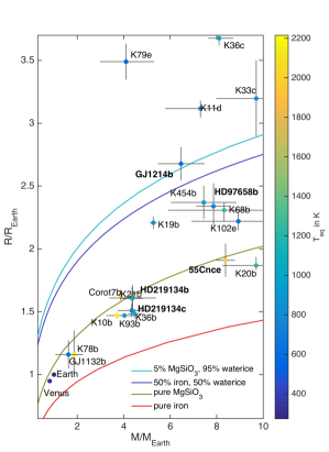
Figure 1: Mass-radius diagram for planets below 2.7 R_⊕ and 10 M_⊕ and mass uncertainties better than 20% in general. HD 219134 b and c are among the coolest exoplanets yet detected regarding their equilibrium temperature (in color). Planets in bold face are included in the comparative study in section 3.3.

2 Methodology

2.1 Interior characterization

Using the generalized Bayesian inference analysis of Dorn et al. (2016a) that employs a Markov chain Monte Carlo (McMC) method, we rigorously quantify the degeneracy of the following interior parameters for a general planet:

• core: core size ($r_{\rm core}$),

• mantle: mantle composition (${\rm Fe}/{\rm Si}_{\rm mantle}$, ${\rm Mg}/{\rm Si}_{\rm mantle}$) and size ($r_{\rm mantle}$),

• water: water mass fraction ($m_{\rm water}$),

• gas: intrinsic luminosity ($L_{\rm env}$), gas mass ($m_{\rm env}$), and metallicity ($Z_{\rm env}$).

From the posterior distribution of those interior parameters, we can compute the posterior distribution of the thickness of a possible gas layer ($r_{\rm env}$), which we then use to infer if the gas layer is hydrogen-rich or poor (Section 2.3). Regarding the volatile-rich layers, our parameterization allows us to produce planet structures that range from (1) purely-rocky to (2) thick water layers with no additional gas layer to (3) thick gas layers without water layers below. The latter structure (3) determines the largest values of $r_{\rm env}$. Figure 2 illustrates the interior parameters of interest.

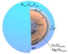
Figure 2: Illustration of interior parameters: core size ($r_{\rm core}$), mantle composition (${\rm Fe}/{\rm Si}_{\rm mantle}$, ${\rm Mg}/{\rm Si}_{\rm mantle}$), mantle size ($r_{\rm mantle}$), water mass fraction ($m_{\rm water}$), intrinsic luminosity ($L_{\rm env}$), gas mass ($m_{\rm env}$), gas metallicity ($Z_{\rm env}$), and atmospheric thickness ($r_{\rm env}$).

The considered data comprise:

• mass $M$,

• radius $R$,

• bulk abundance constraints on ${\rm Fe}/{\rm Si}_{\rm bulk}$ and ${\rm Mg}/{\rm Si}_{\rm bulk}$, and minor elements Na, Ca, Al,

• semi-major axes $a$,

• stellar irradiation (namely, effective temperature $T_{\rm eff}$ and stellar radius $R_{\star}$).

For ${\rm Fe}/{\rm Si}_{\rm bulk}$, ${\rm Mg}/{\rm Si}_{\rm bulk}$ and minor elements, we use their equivalent stellar ratios as proxies that can be measured in the stellar photosphere (Dorn et al., 2015).

The prior distributions of the interior parameters are listed in Table 1. The priors are chosen conservatively. The cubic uniform priors on $r_{\rm core}$ and $r_{\rm mantle}$ reflect equal weighing of masses for both core and mantle. Prior bounds on ${\rm Fe}/{\rm Si}_{\rm mantle}$ and ${\rm Mg}/{\rm Si}_{\rm mantle}$ are determined by the host star’s photospheric abundance proxies. Since iron is distributed between core and mantle, ${\rm Fe}/{\rm Si}_{\rm bulk}$ only sets an upper bound on ${\rm Fe}/{\rm Si}_{\rm mantle}$. A log-uniform prior is set for $m_{\rm env}$ and $L_{\rm env}$. A uniform prior in $Z_{\rm env}$ equally favors metal-poor and metal-rich atmospheres, which seems appropriate for secondary atmospheres. In Section 3.1, we investigate the effect of different priors on $Z_{\rm env}$.

In this study, the planetary interior is assumed to be composed of a pure iron core, a silicate mantle comprising the oxides Na₂O–CaO–FeO–MgO–Al₂O₃–SiO₂, pure water layer, and an atmosphere of H, He, C, and O.

The structural model for the interior uses self-consistent thermodynamics for core, mantle, high-pressure ice, and water ocean, and to some extent also atmosphere. For the core density profile, we use the equation of state (EoS) fit of iron in the hcp (hexagonal close-packed) structure provided by Bouchet et al. (2013) on ab initio molecular dynamics simulations. We assume a solid state iron, since the density increase due to solidification in the Earth’s core is small (0.4 g/cm3, or 3%) (Dziewonski & Anderson, 1981). For the silicate mantle, we compute equilibrium mineralogy and density as a function of pressure, temperature, and bulk composition by minimizing Gibbs free energy (Connolly, 2009). For the water layers, we follow Vazan et al. (2013) using a quotidian equation of state (QEOS) and above 44.3 GPa, we use the tabulated EoS from Seager et al. (2007) that is derived from DFT simulations. Depending on pressure and temperature, the water can be in solid, liquid or vapour phase. We assume an adiabatic temperature profile within core, mantle, and water layers. The surface temperature of the water layer is set equal to the temperature of the bottom of the gas layer.

For the gas layer, we solve the equations of hydrostatic equilibrium, mass conservation, and energy transport. For the EoS of elemental compositions of H, He, C, and O, we employ the CEA (Chemical Equilibrium with Applications) package (Gordon & McBride, 1994), which performs chemical equilibrium calculations for an arbitrary gaseous mixture, including dissociation and ionization and assuming ideal gas behavior. The metallicity $Z_{\rm env}$ is the mass fraction of C and O in the gas layer, which can range from 0 to 1. For the gas layer, we assume an irradiated layer on top of a convective-dominated envelope, for which we assume a semi-gray, analytic, global temperature averaged profile (Guillot et al., 2010; Heng et al., 2014). The boundary between the irradiated layer and the underlying envelope is defined where the optical depth in visible wavelength is $100/\sqrt{3}$ (Jin et al., 2014). Within the envelope, the usual Schwarzschild criterion is used to distinguish between convective and radiative layers. The planet radius is defined where the chord optical depth becomes 0.56 (Lecavelier des Etangs et al., 2008).

We refer to model I in Dorn et al. (2016a) for more details on both the inference analysis and the structural model.

Table 1: Prior ranges.

parameter	prior range	distribution
$r_{\rm core}$	(0.01 – 1) $r_{\rm mantle}$	uniform in $r_{\rm core}^{3}$
${\rm Fe}/{\rm Si}_{\rm mantle}$	0 – ${\rm Fe}/{\rm Si}_{\rm star}$	uniform
${\rm Mg}/{\rm Si}_{\rm mantle}$	${\rm Mg}/{\rm Si}_{\rm star}$	Gaussian
$r_{\rm mantle}$	(0.01 – 1) $R$	uniform in $r_{\rm mantle}^{3}$
$m_{\rm water}$	0 – 0.98 $M$	uniform
$m_{\rm env}$	0 – $m_{\rm env,max}$	uniform in log-scale
$L_{\rm env}$	$10^{18}-10^{23}$ erg/s	uniform in log-scale
$Z_{\rm env}$	0 – 1	uniform

2.2 Estimating the threshold thickness $\Delta R$ of a primordial atmosphere layer considering atmospheric escape

We approximate $\Delta R$ by the atmospheric layer thickness that corresponds to the accumulated mass of hydrogen that may be lost over the planet’s lifetime ($M_{\rm env,lost}$). Loss rates are determined by X-ray irradiation from the star and mass-loss efficiencies. Hydrostatic balance is used to calculate the layer thickness $\Delta R$ corresponding to a primordial atmosphere of mass $M_{\rm env,lost}$. The detailed calculation of $\Delta R$ involves several steps, that are discussed in the following.

Let the layer thickness $\Delta R$ be the difference in radius attributed to a primordial atmosphere. If we assume this layer to be in hydrostatic equilibrium, then this difference in radius is

$$\Delta R=H\ln{\left(\frac{P_{\rm b}}{P_{\rm t}}\right)},$$ (1)

where $H$ is pressure scale height and $P_{\rm b}$ is the pressure at the bottom of the layer, which we will derive in the next paragraphs. $P_{\rm t}$ is the pressure at the top of the layer, corresponding to the transit radius (Heng, 2016),

$$P_{\rm t}\approx\frac{g}{\kappa}\sqrt{\frac{H}{2\pi R}}.$$ (2)

If we assume a mean opacity of $\kappa=0.1$ cm² g^-1 (Freedman et al., 2014), then for both the b and c planets we get $P_{\rm t}\approx 1$ mbar.

The pressure scale height $H$ is calculated assuming a hydrogen-dominated layer (mean molecular mass $\mu=2~{}$g/mol) and using the equilibrium temperature $T_{\rm eq}$,

$$H=\frac{T_{\rm eq}R^{*}}{g_{\rm surf}\mu},$$ (3)

where $g_{\rm surf}$ is surface gravity and $R^{*}$ is the universal gas constant (8.3144598 J mol^-1 K^-1). The estimates in Heng (2016) suggest that the assumption of $T=T_{\rm eq}$ is reasonable. Values for $g_{\rm surf}$ and $T_{\rm eq}$ are listed in Tables 2 and 3.

The pressure at the bottom of the layer $P_{\rm b}$ corresponds to the accumulated mass of escaped hydrogen over the planet’s lifetime $M_{\rm env,lost}$,

$$P_{\rm b}=\frac{gM_{\rm env,lost}}{4\pi R^{2}},$$ (4)

which is simply a restatement of Newton’s second law. $M_{\rm env,lost}$ is approximated by atmospheric escape considerations. Dimensional analysis yields an expression for the atmospheric escape rate,

$$\dot{M}=\frac{\pi\eta F_{\rm X}R^{2}}{E_{g}},$$ (5)

where $F_{\rm X}$ is the X-ray flux of the star and $E_{g}=GM/R$ is the gravitational potential energy. The evaporation efficiency, $\eta$, is the fraction of the input stellar energy that is converted to escaping outflow from the planet. It is often assumed to be a constant, but it is more likely that its value varies with the age of the system (Owen & Wu, 2013). The evaporation efficiency $\eta$ has been studied by various authors (e.g., Shematovich et al., 2014; Salz et al., 2016), who demonstrate that values between 0.01 and 0.2 are reasonable for our planet range of interest. In other words, $\eta$ hides the complexity of atmospheric radiative transfer of X-ray photons as well as unknown quantities such as the planetary albedo.

The strongest assumption we make is that mass loss is constant over the planet’s lifetime, such that $M_{\rm env,lost}=t_{\star}\dot{M}$ ($t_{\star}=12.9$ Gyr; Takeda et al. 2007). Thus, equations 4 and 5 provide us the expression

$$P_{\rm b}=\frac{\eta L_{\rm X}t_{\star}}{16\pi a^{2}R},$$ (6)

with $L_{\rm X}=4\pi a^{2}F_{\rm X}=4\times 10^{26}$ erg s^-1 (Porto de Mello et al., 2006) being the X-ray luminosity of the star. In Figure 3, we compute $\Delta R/R$ as a function of $\eta$, since the exact value of $\eta$ is not well known. Fortunately, $\Delta R/R$ depends weakly on $\eta$. Also, uncertainty in stellar age only has a small effect on $\Delta R/R$: a difference in stellar age of 1 Gyr only introduces variations on $\Delta R/R$ of less than one percent. The spread in $\Delta R/R$ is mainly due to the uncertainties in planetary mass and radius.

The physical interpretation of the preceding expressions for $P_{\rm b}$ and $\Delta R$ are worth emphasizing. The former is the amount of primordial atmosphere that may be lost by atmospheric escape during the lifetime of the star. It provides a conservative estimate, because we have assumed the X-ray luminosity to be constant, whereas in reality stars tend to be brighter in X-rays earlier in their lifetimes:

$$M_{\rm env,lost}=\int_{0}^{t_{\star}}\dot{M}(t)dt>\dot{M}t_{\star}\,.$$ (7)

The expression for $\Delta R$ is then a lower limit for a primordial atmosphere thickness corresponding to this atmospheric mass loss scenario.

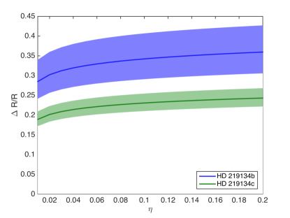
Figure 3: Threshold thickness $\Delta R$ as a function of evaporation efficiency $\eta$. The spread accounts for the uncertainty in planet mass and radius, and age. If the inferred radius $r_{\rm env}$ is less than $\Delta R$, then the atmosphere is most likely enriched and not dominated by H₂.

2.3 Assessing secondary/ primordial nature of an atmosphere

We wish to compare $\Delta R$ with the gas thickness $r_{\rm env}$ inferred from the interior characterization. There are three possible scenarios:

• $r_{\rm env}>\Delta R$: Atmospheric escape is not efficient enough in removing a possible primordial atmosphere. This suggests that a large portion of the atmosphere can be primordial. However, a secondary atmosphere is also possible.

• $r_{\rm env}\approx\Delta R$: Mass loss can be still ongoing and no conclusion can be drawn about the nature of the atmosphere.

• $r_{\rm env}<\Delta R$: Atmospheric escape should have efficiently removed any primordial H₂ atmosphere. If a finite $r_{\rm env}/{R}$ is inferred, the atmosphere is likely enriched and thus of secondary origin. Since the calculation of the threshold thickness $\Delta R$ is conservative, this is the only scenario that can be used for a conclusive statement on the atmospheric origin.

  This conclusion is illustrated in Figure 4, where the time-evolutions of H₂-dominated atmosphere thicknesses for HD219134 b are shown for $\eta=0.01$. The curves are constructed such that at $t=t_{\star}$ the relative thicknesses $r_{\rm env}/{R}$ are equal to 0 (blue), 0.1 (black), 0.17 (red), and 0.23 (green). Furthermore, the solid curves include the time-evolution of X-ray flux, which we assume here to be solar-like ($F_{\rm X}\propto t^{-1.83}$ for $t>t_{\rm sat}$ and $F_{\rm X}=F_{\rm X}$ for $t<t_{\rm sat}$, where the saturation time is equal to 100 Myr and $F_{\rm X}(t_{\star})$ is the observed value) (Ribas et al., 2005). Compared to a constant X-ray flux, the higher stellar activity for a young star implies that an atmosphere thickness of $r_{\rm env}/{R}$ at $t_{\star}$ must have started with a higher gas fraction at $t=0$ (see difference between solid and dashed curves in Figure 4). In both scenarios, we find that the smaller the observed thickness $r_{\rm env}/{R}$ compared to $\Delta R/R$, the shorter the time a planet spends with this atmosphere thickness. Thus it is possible for a planet to host remaining small amounts of an initially thick primordial atmosphere that will have a $r_{\rm env}/{R}$ lower than the threshold thickness. However, we find that this state is a very short fraction of the planet’s lifetime, so it is unlikely that the planets we observe with $r_{\rm env}/{R}$ lower than the threshold value will be remnants of thicker primordial atmospheres. In consequence, inferred atmospheres with thicknesses less than $\Delta R/R$ are likely to be enriched (secondary).

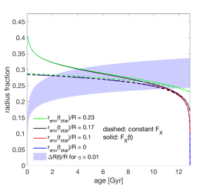
Figure 4: Evolution of H₂-dominated atmosphere thicknesses $r_{\rm env}/{R}$ for HD219134b leading to different thicknesses at $t=t_{\star}$ ($\eta$ = 0.01 in all cases). Solid curves account for a time variable stellar X-ray flux $F_{X}(t)$ (Ribas et al., 2005), whereas dashed curves imply a constant $F_{X}$.The blue-shaded area depicts the evolution of $\Delta R/R$, its spread accounts for the uncertainties in planet mass and radius.

3 Results

3.1 Interiors of HD 219134 b and c

We apply the inferrence method to HD 219134 b and c with the data listed in Tables 2 and 3. The latter lists different stellar abundance estimates from the literature (Mishenina et al., 2015; Ramírez et al., 2007; Valenti & Fischer, 2005; Thévenin, 1998; Thévenin & Idiart, 1999) that were compiled by (Dorn et al., 2016b) to examine different bulk abundance scenarios. Besides a median abundance estimate (V0), they provide an iron-rich (V1) and an iron-poor (V2) scenario, that reflect the limited accuracy in stellar abundance estimates (Table 4). First, we use the median stellar abundance estimate denoted with V0. Figures 5 and 6 show the two and one-dimensional (2-D and 1-D) marginal posteriors for all eight model parameters. Best constrained parameters are the layer thicknesses represented by $m_{\rm water}$, $r_{\rm mantle}$, $r_{\rm core}$. We summarize our findings on the interiors of HD 219134 b and c with respect to the models that fit the data within 1-$\sigma$ uncertainty (blue dots in Figs. 5 and 6):

• The possible interiors of HD 219134 b and c span a large region, including purely rocky and volatile-rich scenarios.

• less than 0.1% of the model solutions for planets b and c, repectively, are rocky ($r_{rocks}$/R $>$ 0.98).

• The possible water mass fraction of HD 219134 b and c can reach from 0 – 0.2 and 0 – 0.1, respectively.

• Unsurprisingly, the individual atmosphere properties ($m_{\rm env}$, $L_{\rm env}$, $Z_{\rm env}$) are weakly constrained. Consequently, their pdfs are dominated by prior information. However, the possible range of atmosphere thickness is well constrained to 0 – 0.18 and 0 – 0.13 for planets b and c, respectively (see Section 3.1.1).

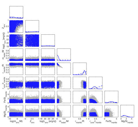
Figure 5: Sampled two and one-dimensional marginal posterior for HD 219134 b interior parameters: gas mass $m_{\rm env}$, gas metallicity $Z_{\rm env}$, intrinsic luminosity $L_{\rm env}$, mass of water $m_{\rm water}$, radius of rocky interior $r_{\rm mantle}$, core radius $r_{\rm core}$, and mantle’s relative abundances ${\rm Fe}/{\rm Si}_{\rm mantle}$ and ${\rm Mg}/{\rm Si}_{\rm mantle}$. Blue dots explain the data within 1-$\sigma$ uncertainty. Dashed curves represent the prior distributions assumed.

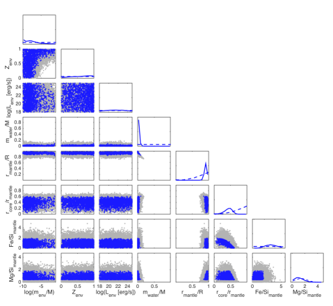
Figure 6: Sampled two-dimensional (2-D) marginal posterior for HD 219134 c interior parameters: gas mass $m_{\rm env}$, gas metallicity $Z_{\rm env}$, intrinsic luminosity $L_{\rm env}$, mass of water $m_{\rm water}$, radius of rocky interior $r_{\rm mantle}$, core radius $r_{\rm core}$, and mantle’s relative abundances ${\rm Fe}/{\rm Si}_{\rm mantle}$ and ${\rm Mg}/{\rm Si}_{\rm mantle}$. Blue dots explain the data within 1-$\sigma$ uncertainty. Dashed curves represent the prior distributions assumed.

Table 2: Summary of planetary data (Motalebi et al., 2015; Gillon et al., 2017).

parameter	HD 219134 b	HD 219134 c
$R$/R⊕	1.606$\pm$0.086	1.515 $\pm$ 0.047
$M$/M⊕	4.36$\pm$0.44	4.34 $\pm$ 0.22
$g_{\rm surf}$[cm/$s^{-2}$]	1656	1865
$T_{\rm eq}$ [K]	1025	784
$a$ [AU]	0.038	0.065

Table 3: Summary of stellar data (Motalebi et al., 2015).

parameter	HD 219134
$R_{\rm star}$/Rsun	0.778 $\pm$ 0.005
$T_{\rm eff}$ in K	4699 $\pm$ 16
$[\rm Fe/H]$	0.04–0.84
$[\rm Fe/H]_{median}$	0.13
$[\rm Mg/H]$	0.09–0.37
$[\rm Mg/H]_{median}$	0.32
$[\rm Si/H]$	0.04–0.27
$[\rm Si/H]_{median}$	0.12
$[\rm Na/H]$	0.17–0.32
$[\rm Na/H]_{median}$	0.19
$[\rm Al/H]$	0.16–0.29
$[\rm Al/H]_{median}$	0.23
$[\rm Ca/H]$	0.18–0.25
$[\rm Ca/H]_{median}$	0.21

Table 4: Considered planet bulk abundance cases. V0 represents median abundance estimates, whereas V1 and V2 refer to iron-rich and iron-poor cases, respectively.

parameter		V0	V1	V2
${\rm Fe}/{\rm Si}_{\rm bulk}$		1.73$\pm$1.55	10.68$\pm$1.55	1.00$\pm$1.55
${\rm Mg}/{\rm Si}_{\rm bulk}$		1.44$\pm$0.91	1.02$\pm$0.91	1.14$\pm$0.91
Na2O [wt%]		0.021	0.01	0.025
Al2O3 [wt%]		0.055	0.023	0.057
CaO [wt%]		0.021	0.01	0.021

3.1.1 Influence of stellar abundances

Dorn et al. (2016b) investigated the influence of different bulk abundance constraints on interior estimates. In Figures 7 and 8, we similarly show this influence on key interior parameters ($r_{\rm env}/{R}$, $m_{\rm water}$, $r_{\rm mantle}$, and $r_{\rm core}$) for the median abundance estimate (V0, blue), the iron-rich case (V1, light green), and the iron-poor case (V2, dark green) (Table 4). As discussed by Dorn et al. (2016b), the largest effects are seen on $r_{\rm mantle}$ and $r_{\rm core}$: if the planets are iron-rich, the core size is significantly larger, which implies a smaller rocky interior ($r_{\rm mantle}$) in order to fit mass. The effect on $r_{\rm env}/{R}$ is apparent in the comparison between the iron-rich case V1 and V0. For an iron-rich planet, the density of the rocky interior is higher. In order to fit the mass, $r_{\rm mantle}$ is smaller. Consequently, to fit the radius, $r_{\rm env}/{R}$ can be larger. For the iron-rich case (V1), the upper 99% percentile of $r_{\rm env}/{R}$ is 0.02 (HD 219134 b) and 0.04 (HD 219134 c) larger than for V0. Even if the iron-rich case is in agreement with spectroscopic data, we believe that V1 may represent a limitation in accuracy rather than the actual planet bulk abundance.

3.1.2 Influence of data uncertainty

In Figures 7 and 8, we also investigate the improvement in constraining interior parameters assuming the hypothetical case of having double the precision on (1) observed mass (light purple), and (2) mass and radius (dark purple). Significant improvement in constraining interior parameters is only obvious for HD 219134 b when both mass and radius precision is doubled. For HD 219134 c, the increase in both mass and radius uncertainty leads to only moderate improvement of parameter estimates. The different potential to improve interior estimates by reducing data uncertainty for planets b and c stems from the fact, that the uncertainties are much smaller for planet c ($\sigma_{R}=3.1\%$) compared to b ($\sigma_{R}=5.4\%$). For the considered planets, improved constraints for interior parameters are dominantly gained by a better precision in radius. This is expected, since mass-radius curves flatten out at higher masses (Fig. 1).

3.1.3 Influence of prior on $Z_{\rm env}$

We have shown that the individual parameters $L_{\rm env}$, $Z_{\rm env}$, and $m_{\rm env}$ are weakly constrained and thereby are dominated by their prior distributions. However, $r_{\rm env}/{R}$ is well constrained (Figures 7 and 8), which is not explicitly a model parameter in this study. Here, we investigate the effect of different priors on the radius fractions $r_{\rm env}/{R}$. An obvious prior to test is on $Z_{\rm env}$. The prior on gas metallicity can be chosen such that it favors H₂-dominated (uniform in 1/$Z_{\rm env}$) or enriched atmospheres (uniform in $Z_{\rm env}$). In Figures 7 and 8 (comparing blue and dark grey curve), we demonstrate that different priors in $Z_{\rm env}$ have only small effects on the possible distribution of radius fractions $r_{\rm env}/{R}$.

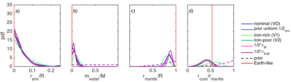
Figure 7: Sampled one-dimensional marginal posterior for selected parameters of HD 219134 b: (a) gas radius fraction $r_{\rm env}/{R}$, (b) water mass fraction $m_{\rm water}$ $/M$, (c) rock radius fraction $r_{\rm mantle}$ $/R$, and (d) relative core radius $r_{\rm core}$/$r_{\rm mantle}$. The posterior distributions depend on precision on bulk abundance constraints (light and dark green curves), and mass and radius uncertainties (light and dark purple curves). For comparison, the Earth-like solution is highlighted in red.

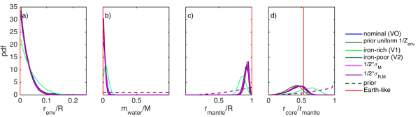
Figure 8: Sampled one-dimensional marginal posterior for selected parameters of HD 219134 c: (a) gas radius fraction $r_{\rm env}/{R}$, (b) water mass fraction $m_{\rm water}$ $/M$, (c) rock radius fraction $r_{\rm mantle}$ $/R$, and (d) relative core radius $r_{\rm core}$/$r_{\rm mantle}$. The posterior distributions depend on precision on bulk abundance constraints (light and dark green curves), and mass and radius uncertainties (light and dark purple curves). For comparison, the Earth-like solution is highlighted in red.

3.2 Secondary or primordial atmosphere?

The comparison in Figure 9 of the inferred $r_{\rm env}/{R}$ (solid lines) to the threshold thickness $\Delta R/R$ (dashed areas) shows that the possible atmospheres of planets b and c are significantly smaller than $\Delta R/R$. This indicates that the possible atmospheres are not dominated by hydrogen but must be secondary in nature. This provides a simple test to identify H₂-rich versus enriched atmospheres, which may then guide future spectroscopic campaigns to characterise atmospheres (e.g., JWST, E-ELT).

3.3 Comparison to other planets

Similarly to HD 219134 b and c, we compare $r_{\rm env}/{R}$ with $\Delta R/R$ (Figure 9 and Table 5) for GJ 1214 b, HD 97658 b, and 55 Cnc e. This serves as a benchmark for our proposed determination for H₂-dominated and enriched atmospheres, since large efforts were put in understanding composition and nature of the atmospheres of the three planets.

For GJ 1214 b, the distribution of $r_{\rm env}/{R}$ is large and overlaps with $\Delta R/R$. The possible atmosphere is consistent with both a H₂-dominated and enriched atmosphere. Prior to our study, much effort has been invested in characterizing the atmosphere of GJ 1214 b (e.g., Berta et al., 2012; Kreidberg et al., 2014). Studies on interior structure suggested either an hydrogen-rich atmosphere that formed by recent outgassing or a maintained hydrogen-helium atmosphere of primordial nature (Rogers & Seager, 2010). A third scenario of a massive water layer surrounded by a dense water atmosphere has been disfavored by Nettelmann et al. (2011) based on thermal evolution calculations that argued that the water-to-rock ratios would be unreasonable large. Transmission spectroscopy and photometric transit observations revealed that the atmosphere has clouds and/or shows features from a high mean-molecular-mass composition (Berta et al., 2012; Kreidberg et al., 2014).

For HD 97658 b, we find that $r_{\rm env}/{R}$ is very likely smaller than $\Delta R/R$. This suggests an atmosphere that is enriched and thus possibly of secondary nature, however, a primordial atmosphere cannot be ruled out with certainty. Previous transmission spectroscopy results of Knutson et al. (2014) are in agreement with a flat transmission spectrum, indicating either a cloudy or water-rich atmosphere. The latter scenario would involve photodissociation of water into OH and H at high altitudes. Evidence for this would be neutral hydrogen escape. Bourrier et al. (2016) undertook a dedicated Lyman-$\alpha$ line search of three transits but could not find any signature. Any neutral hydrogen escape could happen at low rates only. Consequently, a low hydrogen content in the upper atmosphere is a likely scenario. This is consistent with our findings, that a secondary atmosphere is probable.

For 55 Cnc e, our prediction clearly indicates a secondary atmosphere, since $r_{\rm env}/{R}$ is significantly lower than $\Delta R/R$. This is in agreement with previous interpretations based on infra-red and optical observations of transits, occultations, and phase curves (Demory et al., 2012, 2016; Angelo & Hu, 2017). This planet has a large day-night-side temperature contrast of about 1300 K and its hottest spot is shifted eastwards from the substellar point (Demory et al., 2016; Angelo & Hu, 2017). The implication for the atmosphere is an optically thick atmosphere with inefficient heat redistribution. A bare rocky planet is disfavored (Angelo & Hu, 2017). Furthermore, Ehrenreich et al. (2013) give evidence for no extended hydrogen planetary atmospheres (but see Tsiaras et al., 2016). If an atmosphere is present, it would be of secondary nature. Our approximated approach leads to the same conclusion. Furthermore, the study of 55 Cnc e’s thermal evolution and atmospheric evaporation by Lopez (2017) suggest either a bare rocky planet or a water-rich interior. Although the composition of 55 Cnc e is a matter of debate, a hydrogen-dominated atmosphere seems unlikely.

Also we note that this test holds for Earth and Venus, although atmospheric loss mechanisms are very different for them (i.e., Jeans escape and non-thermal escape) (Shizgal et al., 1996). The threshold thicknesses of possible primordial atmospheres are larger than 10 %, whereas the actual thicknesses are no more than a few percent. Thus, our tests would correctly predict a secondary atmosphere for Earth and Venus.

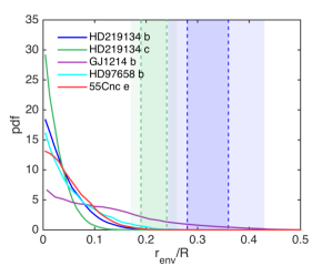
Figure 9: Comparison of $r_{\rm env}/{R}$ between five highlighted planets in Figure 1. Inferred radius (solid lines) and approximated threshold thicknesses $\Delta R/R$ (colored areas with dashed borders). $\Delta R/R$ is listed in Table 5 for all five planets.

Table 5: Threshold thickness $\Delta$R/R for different evaporation efficiencies $\eta$.

planet	Lx [erg/s]	$\Delta R/R$	$\Delta R/R$
		($\eta=0.01$)	($\eta=0.2$)
HD 219134 b	4$\times 10^{26}$	0.28	0.36
HD 219134 c	4$\times 10^{26}$	0.19	0.24
GJ 1214 b	7.4$\times 10^{25}$	0.17	0.22
55 Cnc e	4$\times 10^{26}$	0.37	0.46
HD 97658 b	1.2$\times 10^{28}$	0.18	0.22
Earth	2.24$\times 10^{27}$	0.12	0.16
Venus	2.24$\times 10^{27}$	0.15	0.21

Table 6: Threshold thickness $\Delta$R/R for evaporation efficiencies $\eta$ of 0.01 and 95th-percentile of inferred atmosphere thicknesses $r_{\rm env}/{R}$. ^∗In case of planets for which stellar X-ray luminosities are not available, we assume solar X-ray luminosities.

planet	95th-percentile of $r_{\rm env}/{R}$	$\Delta R/R$
Kepler-78 b	0.15	1.0∗
GJ 1132 b	0.1	0.40∗
Kepler-93 b	$<$0.05	0.31∗
Kepler-10 b	$<$0.05	0.76∗
Kepler-36 b	$<$0.05	0.23∗
HD 219134 c	0.13	0.19
HD 219134 b	0.18	0.28
CoRoT-7 b	0.1	0.59∗
Kepler-21 b	0.05	0.64∗
Kepler-20 b	0.05	0.18∗
55 Cnc e	0.18	0.37
Kepler-19 b	0.27	0.25∗
Kepler-102 e	0.17	0.10∗
HD 97658 b	0.21	0.18
Kepler-68 b	0.28	0.25∗
Kepler-454 b	0.28	0.16∗
GJ 1214 b	0.39	0.17
Kepler-11 d	0.43	0.20∗
Kepler-33 c	0.48	0.18∗
Kepler-79 e	0.58	0.25∗
Kepler-36 c	0.49	0.30∗

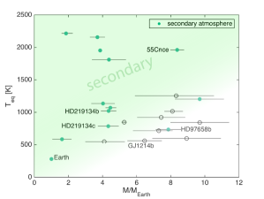
Figure 10: Possible origin of atmospheres depending on effective temperature and planet mass. For labeled planets, we use our method described in the text. For unlabelled planets, stellar X-ray luminosities are not available and thus we assume solar X-ray luminosities which is a fair assumption given that the Kepler mission targeted Sun-like stars. Radii and masses of considered planets are shown in Figure 1.

A comparison of atmospheric origin on a larger set of exoplanets is limited due to the lack of estimated X-ray stellar luminosities. For simplicity, we assume solar X-ray luminosities whenever stellar X-ray luminosities are not available, which is a fair assumption given that the Kepler mission targeted Sun-like stars. Using such simple assumptions, the distribution of planets with secondary atmospheres depends on planet mass and equilibrium temperature to first order (Figure 10 and Table 6). In comparison to the tested HD 219134 b and c, most planets have higher equilibrium temperatures and are thus more vulnerable against atmospheric loss. Also, Dorn et al. (2016b) concluded that it is unlikely that the planets HD 219134 b, Kepler-10 b, Kepler-93 b, CoRoT-7b, and 55 Cnc e could retain a hydrogen-dominated atmosphere against evaporative mass loss.

The possible transition between secondary and primordial atmospheres depending on $T_{\rm eq}$ is positively correlated with planet mass (Figure 10). Theoretical photo-evaporation studies (e.g., Jin et al., 2014; Lopez & Fortney, 2013) and the study on observed planets by Lecavelier des Etangs et al. (2007) predict similar trends, in that planets need to be more massive when receiving higher incident flux in order to retain their primordial atmospheres. For a better understanding of the observed distribution of secondary atmospheres, future estimates of X-ray stellar luminosities are required.

4 Discussion

As already mentioned, the strongest assumption we make is that mass loss is constant over the stellar age. A more accurate approach is to calculate

$$M_{\rm env,lost}=\int_{0}^{t_{\star}}\frac{\pi\eta F_{\rm X}R^{2}}{E_{g}}dt,$$ (8)

where $\eta(t)$ and $F_{\rm X}(t)$ are both functions of time. The X-ray luminosity evolves over the lifetime of the star, which in turn causes the efficiency of atmospheric escape to evolve. Also, the planetary radius $R$ depends on the gas mass fraction that changes over time. We emphasize that, while the $M_{\rm env,lost}=\dot{M}t_{\star}$ approximation may lack precision, the logical structure of our approach is robust and accurate. The reasoning remains that $M_{\rm env,lost}$ (corresponding to a thickness of $\Delta R$) worth of atmosphere may be eroded over the stellar lifetime, so any inferred atmosphere with thicknesses less than this threshold are very unlikely to be primordial (H₂-dominated).

In addition, we assume $T=T_{\rm eq}$ while estimating the threshold thickness (Equation 3). Heng (2016) finds differences on the order of few tens of percents while approximating the scale height with the isothermal scale height at $T=T_{\rm eq}$. If temperatures are higher, the hydrogen escape would be more efficient and $\Delta$R/R would be higher (and vice versa). The uncertainty on the temperature is accounted for by the variability in $\eta$.

Furthermore, our estimates of the radius fraction $r_{\rm env}/{R}$ are subject to our choices of interior model and assumptions. Changes in the interior model, especially the atmosphere model, can affect the estimated $r_{\rm env}/{R}$ as discussed by (Dorn et al., 2016a). Furthermore, we assume distinct layers of core, mantle, water, and gas. This may not be true as discussed for giant planets (Stevenson, 1985; Helled et al., 2010).

Following the outlined strategy, it is possible to test for other types of atmospheres (e.g., N₂ or CO₂-dominated atmospheres). Here, we focussed on an atmosphere type that informs us about formation processes, i.e. we have assumed that a primordial atmosphere is dominated by hydrogen. In principle, a primordial atmosphere can be enriched by planetesimal disruption during the accretion. However, initial gas fractions for super-Earths are small and it is not clear whether atmosphere enrichment can be efficient in these cases nor if metal-enriched thin atmospheres remain well-mixed over long timescales.

We have demonstrated that the possible atmospheres on HD 219134 b and c are very likely to be secondary in nature. We have shown that this result is robust against different assumptions of bulk abundance constraints and prior choices, as shown for $Z_{\rm env}$.

Based on bulk density, both planets could be potentially rocky. However, we would expect planets, that are rocky and that formed within the same disk, to roughly lie on the same mass-radius curve. This is because we expect a compositional correlation, i.e. similar abundances of relative refractory elements (e.g., Sotin et al., 2007). The fact, that HD 219134 b and c do not fall on one mass-radius curve, suggests that the larger planet b must harbor a substantial volatile layer.

Our use of stellar composition as a proxy for the planet bulk composition excludes Mercury-like rocky interiors. If such interiors were applicable to the HD 219134 planets, the rocky interiors would be iron-rich surrounded by substantially thick volatile envelopes in order to fit mass and radius. It remains an open question whether Mercury-like interiors are common or not.

5 Conclusions and Outlook

We have presented a method in order to determine the nature of a possible atmosphere. Since close-in planets suffer from evaporative mass loss, the amount of primordial atmosphere that can be lost is determined by irradiation from the star, lifetime of the system, and evaporation efficiency. Fortunately, the amount of primordial atmosphere loss is weakly dependent on evaporation efficiency and system lifetime in case of the usually Gyr-old observed exoplanets. A comparison between the threshold thickness above which a primordial atmosphere can be retained against atmospheric escape and the actual possible atmosphere thickness is a clear indicator of whether an atmosphere is secondary. We performed this analysis for HD 219134 b and HD 219134 c.

The possible thicknesses of their atmospheres were inferred by using a generalized Bayesian inference method. For this, we have used the data of planet mass, radius, stellar irradiation, and bulk abundance constraints from the star to constrain the interiors of HD 219134 b and c. Interior parameters include core size, mantle composition and size, water mass fraction, intrinsic luminosity, gas mass, and gas metallicity. Although individual parameters of the gas layer ($m_{\rm env}$, $L_{\rm env}$, $Z_{\rm env}$) are only weakly constrained, the thickness is well contrained. Inferred thicknesses $r_{\rm env}/{R}$ are robust against different assumed priors and bulk abundance constraints.

We summarize our findings on HD 219134 b and HD 219134 c below:

• maximum radius fractions of possible gas layers are 0.18 (HD 219134 b) and 0.13 (HD 219134 c),

• the possible atmospheres are likely secondary in nature,

• HD 219134 b must contain a significant amount of volatiles.

Here, we have proposed a simple quantitative determination of the nature of an exoplanetary atmosphere, that does not include spectroscopic measurement. In order to check our method against planets whose atmospheres are intensively studied, we applied it to GJ 1214 b, HD 97658 b, and 55 Cnc e. Our predictions agree with previous findings on their atmospheres, and may be tested by future infrared transmission spectroscopy performed on these exoplanets.

References

- Adams et al. (2008) Adams, E. R., Seager, S., & Elkins-Tanton, L. (2008). The Astrophysical Journal, 673(2), 1160.
- Angelo & Hu (2017) Angelo, I., & Hu, R. (2017). A Case for an Atmosphere on Super-Earth 55 Cancri e. arXiv preprint arXiv:1710.03342.
- Berta et al. (2012) Berta, Z. K., Charbonneau, D., Désert, J. M., Kempton, E. M. R., McCullough, P. R., Burke, C. J., … & Homeier, D. (2012). The Astrophysical Journal, 747(1), 35.
- Bourrier et al. (2016) Bourrier, V., Ehrenreich, D., King, G., Etangs, A. L. D., Wheatley, P. J., Vidal-Madjar, A., … & Udry, S. (2016). Astronomy & Astrophysics, 597, A26.
- Bouchet et al. (2013) Bouchet, J., Mazevet, S., Morard, G., Guyot, F., & Musella, R. (2013). Physical Review B, 87(9), 094102.
- Connolly (2009) Connolly, J.A.D. (2009). Geochemistry, Geophysics, Geosystems, 10(10).
- Demory et al. (2016) Demory, B. O., Gillon, M., De Wit, J., Madhusudhan, N., Bolmont, E., Heng, K., … & Stamenković, V. (2016). Nature, 532(7598), 207-209.
- Demory et al. (2012) Demory, B. O., Gillon, M., Seager, S., Benneke, B., Deming, D., & Jackson, B. (2012). The Astrophysical Journal Letters, 751(2), L28.
- Dorn et al. (2016b) Dorn, C., Hinkel, N.R., Venturini, J. (2016). Astrophysics & Astronomy, 597, A38, 10.1051/0004-6361/201628749.
- Dorn et al. (2015) Dorn, C., Khan, A., Heng, K., Connolly, J.A.D., Alibert, Y., Benz, W., and Tackley, P., (2015). Can we constrain the interior structure of rocky exoplanets from mass and radius measurements?, Astrophysics & Astronomy, 577, A83, 10.1051/0004-6361/201424915.
- Dorn et al. (2016a) Dorn, C., Venturini, J., Khan, A., Heng, K., Alibert, Y., Helled, R., Rivoldini, A., Benz, W. (2016). Astrophysics & Astronomy, 597, A37, 10.1051/0004-6361/201628708.
- Dressing et al. (2015) Dressing, C. D., & Charbonneau, D. (2015). The Astrophysical Journal, 807(1), 45.
- Dziewonski & Anderson (1981) Dziewonski, A. M., & Anderson, D. L. (1981). Preliminary reference Earth model. Physics of the earth and planetary interiors, 25(4), 297-356.
- Ehrenreich et al. (2011) Ehrenreich, D., & Desert, J. M. (2011). Astronomy & Astrophysics, 529, A136.
- Ehrenreich et al. (2013) Ehrenreich, D., Bourrier, V., Bonfils, X., des Etangs, A. L., Hébrard, G., Sing, D. K., … & Forveille, T. (2012). Astronomy & Astrophysics, 547, A18.
- Elkins-Tanton & Seager (2008) Elkins-Tanton, L. T., & Seager, S. (2008). Ranges of atmospheric mass and composition of super-Earth exoplanets. The Astrophysical Journal, 685(2), 1237.
- Fortney et al. (2013) Fortney, J. J., Mordasini, C., Nettelmann, N., Kempton, E. M. R., Greene, T. P., & Zahnle, K. (2013). The Astrophysical Journal, 775(1), 80.
- Freedman et al. (2014) Freedman, R. S., Lustig-Yaeger, J., Fortney, J. J., Lupu, R. E., Marley, M. S., & Lodders, K. (2014). The Astrophysical Journal Supplement Series, 214(2), 25.
- Gillon et al. (2017) Guillot, M., Demory, B.-O. , Van Grootel, V., Motalibi, F., Lovis, C., Cameron, A.C., Charbonneau, C., Latham, D., Molinari, E., Pepe, F.A., Ségransan, D. , Sasselov, D., & Udry, S. (2016). Nature Astronomy, 2017, 1, 56
- Gordon & McBride (1994) Gordon, S., & McBride, B. (1994). Computer program for calculation of complex chemical equilibrium compositions and applications. Cleveland, Ohio, Springfield, Va: National Aeronautics and Space Administration, Office of Management, Scientific and Technical Information Program; National Technical Information Service, distributor
- Guillot et al. (2010) Guillot, T. (2010). Astronomy & Astrophysics, 520, A27.
- Hashimoto et al. (2007) Hashimoto, G. L., Abe, Y., & Sugita, S. (2007). The chemical composition of the early terrestrial atmosphere: Formation of a reducing atmosphere from CI?like material. Journal of Geophysical Research: Planets, 112(E5).
- Helled et al. (2010) Helled, R., Anderson, J. D., Podolak, M., & Schubert, G. (2010). Interior models of Uranus and Neptune. The Astrophysical Journal, 726(1), 15.
- Heng (2016) Heng, K. 2016, ApJL, 826, L16
- Heng et al. (2014) Heng, K., Mendonça, J. M., & Lee, J. M. (2014). The Astrophysical Journal Supplement Series, 215(1), 4.
- Hinkel et al. (2014) Hinkel, N. R., Timmes, F. X., Young, P. A., Pagano, M. D., & Turnbull, M. C. (2014). The Astronomical Journal, 148, 54.
- Hu et al. (2015) Hu, R., Seager, S., & Yung, Y. L. (2015). Helium atmospheres on warm Neptune-and sub-Neptune-sized exoplanets and applications to GJ 436b. The Astrophysical Journal, 807(1), 8.
- Jin et al. (2014) Jin, S., Mordasini, C., Parmentier, V., van Boekel, R., Henning, T., & Ji, J. (2014). The Astrophysical Journal, 795(1), 65.
- Kreidberg et al. (2014) Kreidberg, L., Bean, J. L., Désert, J. M., Benneke, B., Deming, D., Stevenson, K. B., … & Homeier, D. (2014). Nature, 505(7481), 69-72.
- Knutson et al. (2014) Knutson, H. A., Dragomir, D., Kreidberg, L., Kempton, E. M. R., McCullough, P. R., Fortney, J. J., … & Howard, A. W. (2014). The Astrophysical Journal, 794(2), 155.
- Lammer et al. (2013) Lammer, H., Erkaev, N. V., Odert, P., Kislyakova, K. G., Leitzinger, M., & Khodachenko, M. L. (2013). Probing the blow-off criteria of hydrogen-rich ‘super-Earths’. Monthly Notices of the Royal Astronomical Society, 430(2), 1247-1256.
- Lecavelier des Etangs et al. (2007) Lecavelier des Etangs, A. (2007). Astronomy & Astrophysics, 461(3), 1185-1193.
- Lecavelier des Etangs et al. (2008) Lecavelier des Etangs, A., Pont, F., Vidal-Madjar, A., & Sing, D. (2008). Rayleigh scattering in the transit spectrum of HD 189733b. Astronomy & Astrophysics, 481(2), L83-L86.
- Leconte et al. (2015) Leconte, J., Forget, F., & Lammer, H. (2015). Experimental Astronomy, 40(2-3), 449-467.
- Lopez (2017) Lopez, E. D. (2017). Born dry in the photoevaporation desert: Kepler’s ultra-short-period planets formed water-poor. Monthly Notices of the Royal Astronomical Society, 472(1), 245-253.
- Lopez & Fortney (2013) Lopez, E. D., & Fortney, J. J. (2013). The Astrophysical Journal, 776(1), 2.
- Mihalas et al. (1970) Mihalas, D. (1970). Stellar atmospheres. San Francisco, WH Freeman and Co., 1st edition, 1970.
- Miller-Ricci et al. (2009) Miller-Ricci, E., Seager, S., & Sasselov, D. (2009). The atmospheric signatures of super-Earths: how to distinguish between hydrogen-rich and hydrogen-poor atmospheres. The Astrophysical Journal, 690(2), 1056.
- Mishenina et al. (2015) Mishenina, T., Gorbaneva, T., Pignatari, M., Thielemann, F.-K., & Korotin, S. A. (2015). Monthly Notices of the Royal Astronomical Society, 454, 1585
- Motalebi et al. (2015) Motalebi, F., Udry, S., Gillon, M., Lovis, C., Sagransan, D., Buchhave, L. A., …& Rice, K. (2015). The HARPS-N Rocky Planet Search-I. HD 219134 b: A transiting rocky planet in a multi-planet system at 6.5 pc from the Sun. Astronomy & Astrophysics, 584, A72.
- Nettelmann et al. (2011) Nettelmann, N., Fortney, J. J., Kramm, U., & Redmer, R. (2011). The Astrophysical Journal, 733(1), 2.
- Owen & Jackson (2013) Owen, J. E., & Jackson, A. P. (2012). Monthly Notices of the Royal Astronomical Society, 425(4), 2931-2947.
- Owen & Wu (2013) Owen, J. E., & Wu, Y. (2013). The Astrophysical Journal, 775(2), 105.
- Porto de Mello et al. (2006) Porto de Mello, G., del Peloso, E.F., & Ghezzi, L. (2006). Astrobiology, 6, 308
- Ramírez et al. (2007) Ramírez, I., Prieto, C. A., & Lambert, D. L. (2007). Astronomy & Astrophysics, 465, 271
- Ribas et al. (2005) Ribas, I., Guinan, E. F., Guedel, M., & Audard, M. (2005). The Astrophysical Journal, 622(1), 680.
- Rogers et al. (2015) Rogers, L. A. (2015). The Astrophysical Journal, 801(1), 41.
- Rogers & Seager (2010) Rogers, L. A., & Seager, S. (2010). The Astrophysical Journal, 716(2), 1208.
- Salz et al. (2016) Salz, M., Schneider, P. C., Czesla, S., & Schmitt, J. H. M. M. (2016). Astronomy & Astrophysics, 585, L2.
- Schaefer & Fegley (2007) Schaefer, L., & Fegley, B. (2007). Outgassing of ordinary chondritic material and some of its implications for the chemistry of asteroids, planets, and satellites. Icarus, 186(2), 462-483.
- Seager et al. (2007) Seager, S., Kuchner, M., Hier-Majumder, C. A., & Militzer, B. (2007). The Astrophysical Journal, 669(2), 1279.
- Shematovich et al. (2014) Shematovich, V. I., Ionov, D. E., & Lammer, H. (2014). Astronomy & Astrophysics, 571, A94.
- Shizgal et al. (1996) Shizgal, B. D., & Arkos, G. G. (1996). Reviews of Geophysics, 34(4), 483-505.
- Sotin et al. (2007) Sotin, C., Grasset, O., & Mocquet, A. (2007). Icarus, 191(1), 337.
- Stevenson (1985) Stevenson, D. J. (1985). Cosmochemistry and structure of the giant planets and their satellites. Icarus, 62(1), 4-15.
- Takeda et al. (2007) Takeda, G., Ford, E. B., Sills, A., Rasio, F. A., Fischer, D. A., & Valenti, J. A. (2007). The Astrophysical Journal Supplement Series, 168(2), 297.
- Thévenin (1998) Thevenin, F. 1998, Chemical Abundances in Late-Type Stars (VizieR On-line Data Catalog).
- Thévenin & Idiart (1999) Thévenin, F., & Idiart, T. P. (1999). The Astrophysical Journal, 521, 753.
- Thiabaud et al. (2015) Thiabaud, A., Marboeuf, U., Alibert, Y., Leya, I., & Mezger, K. (2015). Astronomy & Astrophysics, 580, A30.
- Tsiaras et al. (2016) Tsiaras, A., Rocchetto, M., Waldmann, I. P., Venot, O., Varley, R., Morello, G., … & Tennyson, J. (2016). Detection of an atmosphere around the super-Earth 55 Cancri e. The Astrophysical Journal, 820(2), 99.
- Valenti & Fischer (2005) Valenti, J. A., & Fischer, D. A. (2005). The Astrophysical Journal Supplement Series, 159, 141.
- Vazan et al. (2013) Vazan, A., Kovetz, A., Podolak, M., & Helled, R. (2013). Monthly Notices of the Royal Astronomical Society, stt1248.
- Venturini et al. (2016) Venturini, J., Alibert, Y., & Benz, W. (2016). arXiv preprint arXiv:1609.00960.
- Vogt et al. (2015) Vogt, S. S., Burt, J., Meschiari, S., Butler, R. P., Henry, G. W., Wang, S., … & Keiser, S. (2015). The Astrophysical Journal, 814(1), 12.
- Zahnle et al. (2015) Zahnle, K., Schaefer, L., & Fegley, B. (2010). Earth?s earliest atmospheres. Cold Spring Harbor perspectives in biology, 2(10), a004895.