Turbulence appearance and non-appearance in thin fluid layers

Abstract

Flows in fluid layers are ubiquitous in industry, geophysics and astrophysics. Large-scale flows in thin layers can be considered two-dimensional (2d) with bottom friction added. Here we find that the properties of such flows depend dramatically on the way they are driven. We argue that wall-driven (Couette) flow cannot sustain turbulence at however small viscosity and friction. Direct numerical simulations (DNS) up to the Reynolds number $Re=10^{6}$ confirm that all perturbations die in a plane Couette flow. On the contrary, for sufficiently small viscosity and friction, we show that finite perturbations destroy the pressure-driven laminar (Poiseuille) flow. What appears instead is a traveling wave in the form of a jet slithering between wall vortices. For $10^{4}<Re<5\cdot 10^{4}$, the mean flow has remarkably simple structure: the jet is sinusoidal with a parabolic velocity profile, vorticity is constant inside vortices, while the fluctuations are small. At higher $Re$ strong fluctuations appear, yet the mean traveling wave survives. Considering the momentum flux barrier in such a flow, we derive a new scaling law for the $Re$-dependence of the friction factor and confirm it by DNS.

Century and a half of ever-expanding studies of turbulence onset in three-dimensional (3d) channel and pipe flows brought a wealth of fundamental and practical knowledge, see e.g. Rev and the references therein. The wall-driven flow is always linearly stable, while the bulk-force-driven flow can be linearly unstable for Reynolds numbers large enough Lin ; OK . Notwithstanding this difference and irrespective of linear stability, all flows undergo transition to turbulence at sufficiently high Reynolds numbers when finite-amplitude perturbations persist Rev . In a pipe flow, some perturbations can take a form of traveling waves of finite amplitude FE ; WK ; BH1 , yet all patterns are unstable and transient, so that the 3d flow is quite irregular already at moderate Reynolds numbers HH ; Rev .

In contrast, for quasi-two-dimensional channel flows it is not even known if they are able to produce turbulence at all. This is despite a rapidly expanding interest in such flows motivated by the needs of industry, astrophysics, geophysics, and laboratory experiments in fluid layers and soap films (see e.g. soap1 ; soap2 , the recent collection PhysFluids and the numerous references therein). To the best of our knowledge, in all experiments in layers and films, external forces and obstacles of elaborate geometry were needed to produce turbulence (see e.g. Pinaki ), and it is not known if such turbulence is able to sustain itself in a channel flow past an obstacle. The reason is that 2d ideal hydrodynamics conserves two quadratic invariants, energy (squared velocity) and enstrophy (squared vorticity). Force at intermediate scales can generate two-cascade turbulence with energy/enstrophy cascading respectively upscales/downscales. On the contrary, the input is at the largest scale in a wall or pressure-driven channel flow, so that it is apriori unclear what kind of turbulence, if any, can exist in the limit of low viscosity and friction.

In this work, combining analytic theory and DNS, we answer this fundamental question. We find out when and how turbulence appears in pressure-driven flows: as “snake” — a traveling wave in the form of a jet meandering between counter-rotating vortices and preserving its form even for strong fluctuations, as shown in Figure 1. Even more remarkably, we find that wall-driven flows remain laminar forever. Both findings substantially widen our fundamental perspective on turbulence and may lead to diverse practical applications.

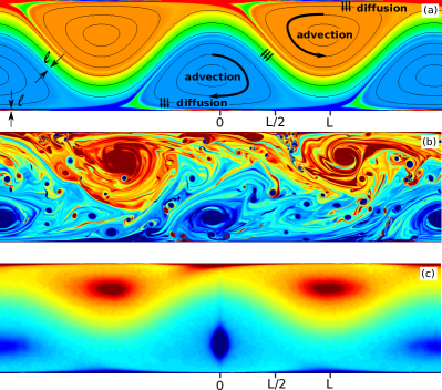
Figure 1: Pressure-driven flows at moderate and large Reynolds number. Vorticity snapshot for (a) $Re=1.89\cdot 10^{4}$ with streamlines, (b) $Re=3.92\cdot 10^{5}$; (c) vorticity averaged over 7000 snapshots over propagation distance $1400L$ in the frame of the negative vortex for $Re=3.92\cdot 10^{5}$.

Turbulence appearance and non-appearance in two-dimensional hydrodynamics probably can be best illuminated by considering interplay between momentum and vorticity, bearing in mind that vorticity is the velocity derivative across a uni-directional flow. Convection carries vorticity unchanged while viscosity diffuses it, so that any turbulence must lead to vorticity mixing and homogenization. We thus expect the mean vorticity profile in a turbulent flow (outside viscous boundary layers at the walls) to be more flat than the laminar profile. On the other hand, turbulence transfers momentum better than a laminar flow, thus increasing drag and decreasing velocity in the bulk. These two requirements are in a perfect agreement for pressure-driven flows where turbulence flattens both the velocity and vorticity mean profiles. On the contrary, the mean velocity profile is monotonous for wall-driven flows, so decreasing velocity in the bulk while keeping it at the walls would make the vorticity profile more non-uniform. We then conclude that momentum and vorticity requirements on turbulence in 2d wall-driven flows are contradictory.

Large-scale flows in thin layers can be effectively described as two-dimensional with bottom friction added. Consider 2d Navier-Stokes equation with unit density and the uniform friction rate $\alpha$:

$$\partial_{t}{\bm{v}}+({\bm{v}}\cdot\nabla){\bm{v}}=\nu\Delta{\bm{v}}-\nabla p-\alpha{\bm{v}},\quad\nabla\cdot{\bm{v}}=0.$$ (1)

Already for the simplest frictionless case (relevant e.g. for flows on superhydrophobic surfaces Rot or soap films under low air pressure) dramatic difference from the three-dimensional case is apparent. Denote $u,v$ the fluctuating velocity components respectively parallel and perpendicular to the mean flow $U(y)$ directed parallel to the walls, which are placed at $y=\pm L/2$ and move with $\pm V/2$. Temporal average of (1) with $\alpha=0$ can be written using vorticity: $\omega=\nabla\times{\bm{v}}$ and $\Omega=-\partial_{y}U$

$$\partial_{y}(\nu\Omega+\langle uv\rangle)=\nu\Omega_{y}-\langle v\omega\rangle=-\partial_{x}\langle p\rangle=A.$$ (2)

Turbulence adds extra fluxes of horizontal momentum and vorticity, related by the Taylor theorem: $\partial_{y}\langle uv\rangle=-\langle v\omega\rangle$. We see that with zero pressure gradient $A$, presence of turbulence would absurdly mean that the vorticity flows against the mean vorticity gradient. One can also argue that the laminar profile $U=Vy/L$ already has a constant vorticity; one cannot excite turbulence to make it more flat. Adding to the viscous flow extra dissipation due to bottom friction could only diminish fluctuations but cannot create them.

These non-rigorous but plausible arguments suggest that a wall-driven flow must relax to the laminar state, $U(y)=V\sinh(y\sqrt{\alpha/\nu})/2\sinh(L\sqrt{\alpha/\nu}/2)$, for any $\nu$ and $\alpha$. That conclusion is supported by DNS whose details are described in the Supplementary Information (SI). Starting from different multi-vortex configurations, we observe different transients and eventual relaxation to the laminar flow. Higher friction makes relaxation more monotonous and controls the relaxation time, while the final energy is determined by $\alpha L^{2}/\nu$, as follows from the laminar solution, see Figure 2. Apparently, the laminar wall-driven flow is the global attractor in two dimensions. To the best of our knowledge, this is the first such example in the whole fluid mechanics.

In thin 3d layers, an ability of moving walls to excite turbulence must depend on the layer thickness $h$. We expect turbulence when the wall Reynolds number $Vh/\nu$ becomes large. How the wall-generated 3d turbulence will be distributed over a wide channel deserves future studies, particularly on account of the tendency of strong planar flows to suppress vertical motions Shats . Note that $\alpha=3\nu/h^{2}$ for planar laminar flows with open surface and no-slip bottom, while vertical motions makes the very notion of $\alpha$ unapplicable.

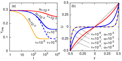
Figure 2: Relaxation of wall-driven flows with $V=1,L=1$ and different viscosities and friction to the laminar profile: (a) RMS velocities as function of time; (b) profiles of saturated flow, indistinguishable from the laminar solution. Initial perturbation had 8 vortex layers and amplitude of 0.1.

From another perspective, impossibility of turbulence in a 2d wall-driven flow can be related to a sign-definite mean vorticity and a mean shear. Even if one initially creates (as we did) vortices of both signs, the opposite-sign vorticity is getting destroyed by the shear while the same-sign vorticity is getting homogenized back into the laminar profile. On the contrary, for the pressure-driven flow, the mean vorticity has opposite signs at opposite walls, so that turbulence cannot homogenize vorticity back to the laminar profile.

We turn now to the pressure-driven flow and define the respective dimensionless control parameters $Re_{A}=A^{1/2}L^{3/2}/\nu$ and $Ru_{A}=A^{1/2}/\alpha L^{1/2}$. Here $A$ has a dimensionality of acceleration (force per unit mass), it is either pressure gradient divided by density or gravity acceleration for soap films.

There is a rich history of modeling 2d Navier-Stokes channel flows with the goal to find threshold $Re$ over which finite perturbations can be sustained, see, e.g. OK ; Jimenez and the references therein. To the best of our knowledge, the largest $Re=10^{4}$ was achieved in Jimenez , where transitional turbulence was observed and it was estimated that fully developed turbulence is to appear around $2\cdot 10^{5}$ which were beyond computer resources back then. Here we explore higher $Re$ never treated before; we also add uniform friction to relate to applications in real fluid layers.

We observe that the transition to the steady-state is slow and can be non-monotonic, some transient behavior is discussed in SI. In all cases we find that pressure-driven flows relax to either of two states: the laminar uni-directional flow or a traveling wave with much slower average flow rate. In the latter case, most of the flux occurs along a sinusoidal jet meandering between two sets of counter-rotating vortices rolling along the walls, Fig. 1. While we cannot rule out that both laminar and sinuous states are long-living meta-stable states (as in 3d pipe flow), we have not seen switches between them once the steady state is established.

The time of transients can be reduced by starting with a low-amplitude, large-scale perturbation to the laminar profile to mimic naturally developing instability (presumably, the one predicted by Lin for the case of $\alpha=0$ Lin ). Then, the early evolution shows well-defined exponential growth, suggesting linear instability. Modeling a $12L$ section of the channel, we applied perturbations with the wavelengths $\lambda_{\rm pert}=3,4,6,12L$ for $Re_{A}=894$ and $Ru_{A}=179$. The largest growth rate $\gamma$ was found for $\lambda_{\rm pert}=4L$, so we used this wavelength for all other simulations; the results are shown in Fig. 3a for different $Re_{A}$ and $Ru_{A}$. The line in the plane $Re_{A}-Ru_{A}$ with zero $\gamma$ separates laminar and sinuous flows in Fig. 3b. Note that friction stabilizes the laminar flow. The inset in Fig. 3 shows the Reynolds number, $Re=\overline{U}L/\nu$, based on the mean flow rate, $\overline{U}$, as a function of $Ru_{A}$ for $Re_{A}=894$. When friction is large ($Ru_{A}$ is small), the flow is laminar. As friction is reduced, the laminar flow becomes faster, yet, at $Ru_{A}\approx 100$ the system transitions to the sinuous state and the flow rate drops. That means that one can speed up the flow by increasing friction, which facilitates transition from the sinuous to the laminar regime.

The long-time evolution of the instability shows that right after the threshold the sinuous flow appears on the scale of the domain, $\lambda=4L$, while at higher $Re_{A},Ru_{A}$ we observe transition to a sinuous flow with wavelength $\lambda=2L$. These long-term states are indicated in Fig. 3a. Reducing dissipation even further, we observe an unsteady, sinuous-like flow with strong fluctuations, which we call “turbulent state”. Below, we take a closer look at these long-term states state for frictionless systems.

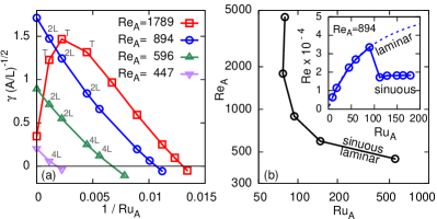
Figure 3: Stability of the pressure-driven flow. (a) The growth rate of perturbations with $\lambda=4L$ versus dimensionless friction for different viscosities. Marks 4L and 2L indicate wavelengths of the long-term sinuous flow, “T” indicates long-term turbulent flow. (b) Stability diagram in the friction-viscosity space. Inset: Reynolds number versus friction.

Without friction, we observe uni-directional Poiseuille flow up to $Re_{A}\approx 500$ and $Re\approx 2\cdot 10^{4}$. At $Re_{A}\approx 500$ the snake is born already with a finite amplitude of modulation (see SI). For $500\lesssim Re_{A}\lesssim 1500$, the flow is a sinuous traveling wave with $10^{4}\lesssim Re\lesssim 5\cdot 10^{4}$ and no noticeable fluctuations. The flow has a beautifully simple stationary structure in a co-moving reference frame: The jet is sinusoidal with a parabolic velocity profile, while vorticity is essentially constant across each vortex, which appears as a plateau in the vorticity cross-sections in Fig. 4a. Constant vorticity inside the vortices can be explained in the spirit of Bat as a consequence of viscosity being very small and yet finite: The former means that vorticity must be constant along the (closed) streamlines, while the latter mean that vorticity must be constant across the streamlines in a stationary flow. The same argument suggests that the flux of vorticity must be constant across the jet, and thus vorticity must change linearly between opposite values at the separatrices.

At $Re_{A}\approx 1500$ the flow becomes turbulent. For $Re_{A}\gtrsim 2000$ and up to 8000 ($Re=3.92\cdot 10^{5}$) the relative level of velocity and vorticity fluctuations remains constant within the accuracy of our measurements. All turbulent flows have a pronounced large-scale structure of a jet and $2L$-periodic chain of vortices, similar to the sinuous flow. This is seen from comparison of Fig. 1a with Fig. 1c, where the averaging is done in the frame of the stronger negative vortex (the other three vortices are blurred to a different degree by fluctuations). In the turbulent state, the chaotic small-scale vortices are created at the walls, pulled out, and eventually each merges into a big vortex of the same sign thus feeding the large-scale flow. While horizontally averaged velocity and vorticity for sinuous and turbulent are of similar shape (see SI for more detail), the time-averaged flows expose qualitative difference: in the turbulent state, mean vorticity peaks at the centers of vortices rather than being flat across the vortex, see Fig. 4 and Fig. 1.

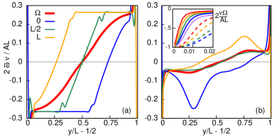
Figure 4: Vorticity $\overline{\omega}(x,y)$ time-averaged in the moving frame of a vortex. Vertical slices are taken through $x=0$, $L/2$, and $L$, as shown in Fig. 1, for $Re_{A}=516$ (a) and $Re_{A}=4000$ (b). The thick red line is zonally averaged vorticity $\Omega(y)=\int\overline{\omega}(x,y)\,dx$. Inset: $\Omega$ in the boundary layer for $Re_{A}=516$, 362, 894, 1265, 2000, 2828, 4000, 5656, and 8000, from bottom to top.

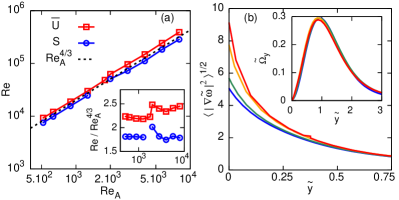
Figure 5: (a) The Reynolds numbers, based respectively on the flow rate $\overline{U}$ and the speed of the traveling wave $S$, versus the Reynolds number based on the applied pressure. Inset: data compensated by $Re^{4/3}$. (b) Fluctuations of the vorticity gradient in the boundary layer for $Re_{A}=8000$, 5656, 4000, and 2828, from top to bottom, in coordinates $\nabla\tilde{\omega}=\nabla\omega Re_{A}^{-2/3}\nu/AL$ and $\tilde{y}=(y/L-1/2)Re_{A}^{2/3}$. Inset: gradient of zonally averaged vorticity in the same coordinates for the same $Re_{A}$.

From the topology of the mean flow profile, depicted in Fig. 1a, we now derive the relation between the applied gradient $A$ and the mean flow rate $\overline{U}$ in the limit of large $Re_{A}=A^{1/2}L^{3/2}/\nu$. For that, one needs to describe the transfer of momentum (or equivalently vorticity) from the center to the walls, taking into account two separatrices, one separating the vortex from the jet and another from the wall boundary layer. Vorticity is diffused by viscosity across the separatrix, then is carried fast by advection inside the vortex, and then transferred by viscosity towards the wall. There are thus two viscous bottlenecks (transport barriers) in this transfer: on the jet-vortex separatrix and on the wall boundary layer. The width $\ell$ of the separatrix boundary layer can be estimated requiring the diffusion time $\ell^{2}/\nu$ to be comparable to the turnover time $L/U$, which gives $\ell\simeq(\nu L/U)^{1/2}$ and the effective viscosity (momentum diffusivity) $\nu_{e}\simeq U\ell\simeq\sqrt{\nu UL}$ (we do not distinguish $U$ and $\overline{U}$ in the estimates). Requiring that the momentum flux due to pressure gradient is carried by the viscosity towards the walls, $A\simeq\nu_{e}U/L^{2}$, we obtain the expressions for the effective Reynolds number and the effective turbulent viscosity:

$$Re={UL\over\nu}\simeq{L^{2}A^{2/3}\over\nu^{4/3}}=Re_{A}^{4/3}\,,\quad\nu_{e}\simeq\nu Re_{A}^{2/3}\ .$$ (3)

To describe the wall boundary layer, note that $v\equiv 0$ at a wall. Therefore, integrating (2) over $y$ from wall to wall, we obtain $\Omega(L/2)=-U^{\prime}(L/2)=AL/2\nu$, that is always equal to the laminar value, see the inset in Fig. 4b. Now we estimate the width of the wall boundary layer, $U/U^{\prime}(L)\simeq LA^{2/3}\nu^{-1/3}/AL\nu^{-1}\simeq\nu^{2/3}/A^{1/3}\simeq\ell$, which confirms that our estimate (3) is self-consistent.

Appearance of the thin boundary layer at large $Re$ (see SI for the details) must lead to a sharp maximum of the vorticity derivative, which we estimate as follows: $\max\Omega_{y}\simeq\Omega(L/2)/\ell\simeq LA^{4/3}\nu^{-5/3}$. That value is much larger than $\Omega_{y}(L/2)=A/\nu$, derived from taking (2) at a wall. Away from the wall boundary layer, turbulence must suppress the mean vorticity gradient, as indeed seen in the insets in Figs 4b and 5b.

In the presence of friction the scaling law (3) is expected to hold when the typical time of the momentum transfer to the wall, $U/A\simeq L(A\nu)^{-1/3}$, is shorter than the friction time $\alpha^{-1}$, otherwise the uniform friction dominates and we have linear regime with $U\propto A$. This means that the pressure acceleration must exceed both viscous and friction thresholds: $A\gg\nu^{2}L^{-3},(\alpha L)^{3}/\nu$.

Numerical simulations support (3), see Figure 5. The scaling $Re\propto Re_{A}^{4/3}$ continues through both regimes, of weakly and strongly fluctuating flows, even though the proportionality constant might be slightly changing at the transition, as seen in the inset in Figure 5a. The mean vorticity profile at the boundary layer also follows the scaling (3), as shown in the inset in Figure 5b plotted for the rescaled quantity $\tilde{\Omega}_{y}=\Omega_{y}(y)/\max\Omega_{y}=\nu\Omega_{y}/ARe_{A}^{2/3}$.

Let us briefly discuss the role of the turbulent fluctuations. Flow dissipates energy and enstrophy, and the viscous dissipation rate of the former is proportional to the latter: $\nu\langle|\nabla v|^{2}\rangle=\nu\langle\omega^{2}\rangle$. It follows from (3) that the work $A\overline{U}$ done by the pressure gradient gives the same estimate as the energy dissipation rate by the mean flow: $\nu\overline{\Omega^{2}}\simeq\nu U^{2}/\ell L\simeq A^{5/3}L\nu^{-1/3}\simeq AU$. This means that the mean flow is able to dissipate energy by itself. Indeed, the DNS data show (see SI, Fig. 2) that the turbulent enstrophy fluctuations are smaller than the enstrophy of the mean flow, while velocity fluctuations are negligible. The dissipation of the second inviscid invariant, enstrophy, is determined by the vorticity gradients shown in Figure 5b. We observe that the mean vorticity gradient follows (3), while the contribution of near-wall fluctuations into the vorticity gradients, and therefore into the enstrophy dissipation, is much larger and grows with $Re$ faster than the vorticity of the mean flow. This suggests that enstrophy is dissipated by turbulence rather than by the mean flow, which deserves future research with much better statistics and resolution.

One can recast (3) as the statement that the friction factor of a 2d “pipe”, $AL/U^{2}$, decays as $Re_{A}^{-2/3}\sim Re^{-1/2}$, which is faster than in three dimensions, where one finds the empirical Blasius law $Re^{-1/4}$ for moderate $Re$ and the logarithmic decay for large $Re$. Within purely 2d system (where separatrix is responsible for the transport barrier), the scaling law (3) may be expected to hold at arbitrary large $Re$, yet in fluid layers its validity is restricted by the requirement that $\ell\simeq LRe_{A}^{-2/3}=LRe^{-1/2}$ exceeds the fluid depth $h$. Therefore, we expect that as $Re$ approaches $(L/h)^{2}$, the decay of the friction factor with $Re$ slows down and eventually converges to the 3d values observed in rectangular ducts FR .

Traveling wave pattern thus enhances effective viscosity and suppresses the flow rate compared to the laminar regime. It is instructive to compare the viscosity enhancement (3) with the enhancement of diffusivity $\kappa$ by the factors $Pe^{1/2}$ for cellular flow Childress ; BS and $Pe^{1/3}$ for wall-attached flow 2/3 , where $Pe=UL/\kappa$. That enhancement of diffusion leads to acceleration of flame fronts NV and other phenomena. Similar to (3), interplay between small noise and advection universally leads to the $1/3$-scaling with noise amplitude: for tumbling frequency of a polymer in a shear flow KoT , for the Lyapunov exponent of an integrable system under stochastic perturbation Kurchan .

To conclude, we have established that wall-driven 2d flow is always laminar. We described the traveling wave pattern which replaces the laminar flow for pressure-driven flows. In distinction from 3d, the traveling wave we find in 2d is stable; as the Reynolds number grows, the fluctuations increase yet the mean flow preserves its traveling-wave “snake” form. Another remarkable property of 2d snake is that it contains separatrices, which modify momentum transport to the walls and thus lead to a new type of scaling law for the friction factor.

We thank A. Obabko for help in using Nek5000. The work was supported by the grants of Israel Science Foundation and the Minerva Foundation and by NSF grant no. DMS-1412140. Simulations are performed at Texas Advanced Computing Center (TACC) using Extreme Science and Engineering Discovery Environment (XSEDE), supported by NSF Grant No. ACI-1548562 through allocation TG-DMS140028.

SUPPLEMENTARY INFORMATION

Numerical setup

We solve the Navier-Stokes equation with bottom friction, Eq. (1) from the main text, using a spectral element code, Nek5000 in the domain $-L/2<y<L/2$, $0<x<L_{x}$ with $L=1$ and periodic boundary conditions in $x$-direction. Unless specified, $L_{x}=4L$. For wall-driven flows, the velocity at the boundaries is $u(x,\pm L/2,t)=\pm u_{w}/2$ with $u_{w}=1$. For pressure-driven flows, no-slip boundary conditions at the walls are used.

Initial velocity has the form ${\bm{v}}(x,y,0)=U_{0}(y){\bf i}_{x}+{\bm{v}}_{0}(x,y)$, with perturbation,

$$u_{0} = -2(a/k_{x})\sin(k_{y}y)\cos(k_{y}y)\sin(k_{x}x),$$ (4)

$$v_{0} = \quad\;(a/k_{y})\sin(k_{y}y)\sin(k_{y}y)\cos(k_{x}x),$$ (5)

where $k_{x}=\pi n/L$, $k_{y}=\pi m/L$ and $n,m=1,2,3...$. Note that the perturbation vanishes at the boundaries, satisfies $\nabla\cdot{\bm{v}}_{0}=0$, and has the structure of vortex layers.

Unless specified, for wall-driven flows we use the mesh of $256\times 80$ elements with 7 collocation points per element in each direction. For pressure-driven flows we use either the same mesh with 7 or 9 collocation points or the mesh of $512\times 160$ elements with 7 collocation points. The size of elements varies in $y$-direction to provide denser mesh near boundaries. The number of collocation points per element in one direction corresponds to the spatial interpolation order. The method is 3rd order accurate in time.

Simulations of wall-driven flows

For the wall-driven flows, the velocity perturbation has been added to the linear velocity profile $U_{0}=u_{w}y/L$. We use vortices with aspect ratio one, $k_{y}=k_{x}=\pi n$, where $n$ corresponds to the number of vortex layers in $y$-direction. We have considered viscosity down to $\nu=10^{-6}$, perturbation amplitudes $a/k_{x}=a/k_{y}=0.1$, $0.5$, and $1.0$, and 4, 8, or 16 vortex layers.

There are interesting transients in the evolution of finite perturbations in the wall-driven flow. At short times, $t\sim 1$, merging of vortices could result in the short-term increase of maximum velocity. One can explain it by linear model: the modulus of the sum of the (non-orthogonal) eigen modes can increase with time even when modes are decaying with different rates. At intermediate times, the flow appears chaotic, yet we clearly observe the upscale energy transfer as the number of vortices reduces with time while their size increases. Some vorticity is generated at the walls and propagates inwards, but this effect weakens with time. In the long term, all perturbations die and the flow approach the laminar solution $U(y)=\frac{u_{0}}{2}\sinh\left[y\sqrt{\frac{\alpha}{\nu}}\right]/\sinh\left[\frac{L}{2}\sqrt{\frac{\alpha}{\nu}}\right]$ of the steady equation $\nu U^{\prime\prime}-\alpha U=0$.

Simulations of pressure-driven flows

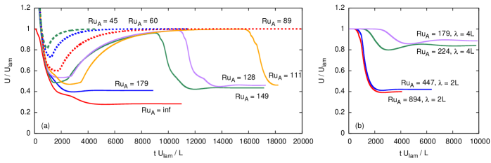
Figure 6: Flow rate $\overline{U}$ in pressure-driven systems with friction for (a) small-scale perturbation on top of parabolic profie for $Re_{A}=894$, and (b) large-scale perturbation on top of laminar profile for $Re_{A}=596$. For all cases in (a) laminar sinuous flows had wavelength $\lambda=2L$; in (b) both $\lambda=2L$ and $\lambda=4L$ were observed. Simulations that evolved to sinuous and laminar flows are shown with solid and dashed lines respectively.

We started with a numerical setup similar to the one for wall-driven flow, except that we have enabled external pressure gradient and set wall velocities to zero. The initial perturbations with $k_{y}=k_{x}=\pi n$, $n=8$, and $a/k_{x}=a/k_{y}=0.1$ or 0.01 were added to $U_{0}=1-4y^{2}$ in the domain with aspect ration $4:1$. We considered $Re_{A}=896$ ($L=1$, $\nu=10^{-5}$, $A=8\times 10^{-5}$) and $Ru_{A}>45$ ($0\leq\alpha\leq 2\times 10^{4}$).

The transient behavior took frustratingly long times and often defied expectations. For instance, in the run for $Ru_{A}=128$ shown in Fig. 6a, we observed a convincing sinuous state reached at $t\approx 1000L/U_{\rm lam}$, where $U_{\rm lam}$ is the laminar flow rate, yet at $t\approx 3000L/U_{\rm lam}$ it started to accelerate toward the laminar state, and it did so until $t\approx 11000L/U_{\rm lam}$, when it started to decelerate. At $t\approx 16000L/U_{\rm lam}$ the system was back to the sinuous state. The evolution in such complex cases is sensitive to the initial conditions. The initial vortices, which have the size of a fraction of the channel, do not evolve directly to the traveling wave solution. These perturbations die, and then the remaining shear flow develops an instability. It occurs for sufficiently high $Re_{A}$ via creation of system-size vortex pair with the wavelength of the length of box, $\lambda_{\rm inst}=4L$, which later transitions to the sinuous solution with shorter wavelength, $\lambda_{\rm wave}=2L$. The transition to the system-size vortex pair can be detected in vertical velocity, as low as 12-14 orders of magnitude below the horizontal component. That means that such systems in reality may be very sensitive to the level of noise and vibrations.

We utilize this mechanism of naturally-developing instability to study stability of the laminar flow with friction. Instead of small-scale vortices, we initially impose a large-scale, small-amplitude perturbation that mimics the early stages of transition from laminar to sinuous flow. In particular, we use a single layer of elongated vortices, $k_{y}=\pi$, $k_{x}=2\pi n/L_{x}$, with the typical amplitude of perturbation $a/\pi=10^{-4}\,u_{0,\rm lam}$, where $u_{0,\rm lam}$ is the velocity at the center of laminar profile. In most simulations, we started with one pair of initial vortices in the box with $L_{x}=4L$; a small number of simulations was done with $n=1,2,3,4$ in the box of $L_{x}=12L$ (and proportionally extended computational grid). The background velocity was given by the laminar profile,

$$u_{\rm lam}(y)=\frac{A}{\alpha}\left(1-\frac{\cosh\sqrt{\frac{\alpha}{\nu}}y}{\cosh\sqrt{\frac{\alpha}{\nu}}\frac{L}{2}}\right),$$ (6)

with the following, based on flow rate, Reynolds number,

$$Re=Re_{A}Ru_{A}\left(1-\sqrt{\frac{4Ru_{A}}{Re_{A}}}\tanh\sqrt{\frac{Re_{A}}{4Ru_{A}}}\right).$$ (7)

Selection of the initial velocity as the laminar flow plus small perturbation produced more regular evolution. Early stages show exponential growth or decay, measured by RMS of vertical velocity. As the perturbation grows, it is transformed into the sinuous flow with the same wavelength $\lambda=4L$ when there is a significant bottom friction, as seen in Figure 7c. At lower bottom friction, the saturated state appears with doubled number of vortices, $\lambda=2L$, seen in Figure 7a,b. It may well be that in an open channel, unrestricted by periodic boundary conditions, the wavelengthes will be different and depend on $Re_{A},Ru_{A}$. In the main text, we present the growth rate for $\lambda=4L$ for $Re_{A}=447$, 596, 894, and 1789, (at $A=8\times 10^{-5}$) and $Ru_{A}<81$, and the stability diagram in $Re_{A}$-$Ru_{A}$ space.

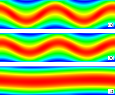
Figure 7: Snapshots of velocity modulus for (a) $Re_{A}=894$, $\alpha=0$ for established traveling wave, (b) $Re_{A}=596$, $Ru_{A}=179$ taken at 70% of the time taken in Fig. 2a, and (c) $Re_{A}=596$, $Ru_{A}=447$ taken at 50% of the time taken in Fig. 2a. In each case, the colormap is scaled between zero and maximum velocity.

$Re_{A}$	$\quad\nu\quad$	$\quad A\quad$	$\quad\overline{U}\quad$	$\quad S\quad$	elements	p	$\;t\overline{U}/L$	n
516	3e-5	2.4e-4	0.278	0.225	256x64	8	5.1	200
632	2e-5	1.6e-4	0.241	0.197	256x64	8	4.8	200
894	1e-5	8.0e-5	0.189	0.156	256x64	8	3.8	200
1264	5e-6	4.0e-5	0.149	0.123	256x64	8	3.0	200
1788	5e-6	8.0e-5	0.242		256x64	8
2000	2e-6	1.6e-5	0.125	0.102	256x80	9	1800	9000
2828	1e-6	0.8e-5	0.096	0.073	256x80	9	1800	9000
4000	1e-6	1.6e-5	0.146	0.111	256x80	9	1800	9000
5656	1e-6	3.2e-5	0.243	0.183	512x160	7	1400	7000
8000	5e-7	1.6e-5	0.196	0.143	512x160	7	1400	7000

Table 1: Parameters of simulations of pressure-driven flows without friction together with obtained flow rate $\overline{U}$ and the speed of the traveling wave $S$. Here, $p$ in the number of collocaton points per spectral element in each direction, $t$ is the time inverval used for averaging, and $n$ is the number of snapshots. In all cases, $L_{y}=L=1$ and $L_{x}=4L$. In simulations with $Re_{A}=5656$ and 8000, 1% damping of hyper viscosity type was applied to the highest mode.

To study the established flows at highest possible Reynolds numbers, we extended selected simulations with $\alpha=0$ to times much longer than a typical time of fluctuations in total energy and enstrophy. Then, we used the final velocity snapshots as initial conditions for runs at higher $Re_{A}$. Summary of simulations is shown in the Table. The table includes simulation parameters, $A$ and $\nu$, information on numerical grids, the resulting flow rate $\overline{U}$ and the speed of the traveling wave $S$, and the time interval and the number of snapshots used for averaging. As discussed in the main text, fluctuations in velocity become noticeable only for $Re_{A}\gtrsim 1500$; these simulations required averaging over long effective propagation distances, $\sim\!10^{3}L$, to collect meaningful statistics. In contrast, to estimate average quantities and the level of fluctuations in saturated sinuous flows with low fluctuations it was sufficient to collect statistics for only several propagation wavelengths.

A natural way to treat appearance of a traveling wave in a parallel flow is to consider a critical layer where the speeds of the flow and the wave coincide. For sufficiently small viscosity and friction, each critical line in 2d is expected to generate a chain of cat-eye vortices of the same sign. As one can see in Figure 8, at small bottom friction, the snake is born with already a finite amplitude of modulation $H$ and cannot be described as a small perturbation of a laminar flow, in spite of a sinusoidal shape of the jet. Moreover, the whole flow is far from being trivial since the boundary layer is quite complicated. The critical line (where the horizontal velocity is equal to the speed of the traveling wave), of course, passes through the vortex centers in the traveling-wave co-moving frame. Yet in between it almost touches the wall, passing through the stagnation point where two separatrices cross: the one separating the vortex from the wall and another from the jet, see Figure 9. Huge velocity gradients are created there, and a very narrow tongue of negative high vorticity separates from the wall and goes along the separatrix up into the bulk. In addition, the stream of high positive vorticity is generated where the vortex rubs against the wall in the direction opposite to that of the jet. On the way up the streams of positive and negative vorticity blend together approximately during one vortex turnover time. A significant future numerical and analytical work will be required to understand and describe this elaborate structure of the traveling-wave flow and its evolution with $Re$. (Note that at the coherent sinuous regime, the jet amplitude $H$ grows, while the width $h$ decreases with the Reynolds number.)

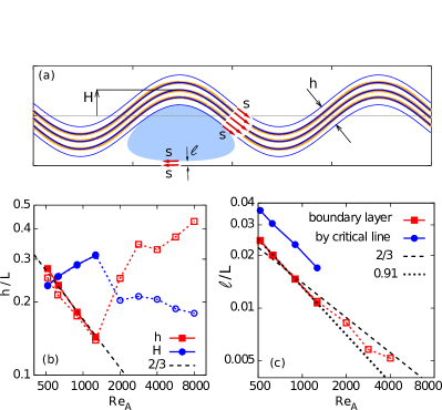
Figure 8: (a)Vorticity level sets $\omega=0$, $\pm\omega_{0}/2$ (orange dots) for $Re_{A}=632$ fitted by $y=H\sin(\pi x/L)+const$ (blue lines). The blue region schematically represents the area of constant vorticity, the red arrows represent the flow. (b) Pressure dependence of the amplitude and the width of the jet. (c) The width of the boundary layer, $\ell$ and the minimal distance of the critical line from the wall. Filled symbols and solid lines are from instant snapshots of the sinuous flow. Empty symbols and dashed lines are from time-averaged snapshots of the turbulent flow, where the level sets $\omega=0$ and $\omega_{2}/2$ were used, $\omega_{2}$ being the maximum vorticity at the vertical slice through the center of positive vortex excluding the boundary layers, $-3/8<y/L<3/8$.

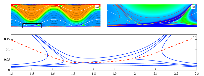
Figure 9: (a) Streamlines (solid) and the critical line (broken) for $Re_{A}=894$ superimposed on the vorticity field with box indicating zoom region shown in (b); (c) Streamlines and the critical line near the stagnation point for $Re_{A}=516$.

The description of the sinuous and turbulent flows are presented in the main text, as well as the discussion of mean flows and fluctuations. The relative values for fluctuations are shown here in Fig. 10. We also supplement the main text with the profiles of the horizontally averaged velocity and vorticity, shown in Fig. 11. The profiles for the two types of flow are of qualitatively the same shape: velocity near the wall has the same slope as the laminar profile for corresponding $Re_{A}$ and vorticity has the same value. Away from the walls, the quantities, normalized to their laminar values, diminish with $Re_{A}$. At the wall, $\Omega$ is very close to the value given by the laminar parabolic profile. Surprisingly, the correction is quadratic in distance, not linear as it would be in classical Poiseuille flow.

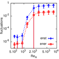
Figure 10: Relative fluctuations in total energy and enstrophy in the reference frame of a moving vortex.

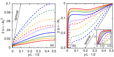
Figure 11: The time averaged and horizontally averaged profiles for (a) velocity for $Re_{A}=516$, 632, 894, 1264, 2000, 2828, 4000, 5656, and 8000 (top to bottom) and (b) vorticity for same $Re_{A}$ (bottom to top). The velocity is rescaled by the laminar velocity at the center and the vorticity is rescaled by the laminar vorticity at the the wall. Sinuous and turbulent solutions are shown with dashed and solid lines respectively.

Ball-bearing model

The remarkably simple structure of the flow as a jet slithering between vortices suggests to treat it with a simple mechanical image of a ball-bearing. The jet, like a string pulled between rolls, rotates the rolls, which like balls in a ball-bearing “lubricate” the system. That allows one to go beyond the scaling and estimate the order-unity numerical pre-factor.

In the main text we have pointed out that the traveling wave observed at moderate $Re$ consists of the jet and vortex cells, as illustrated in Figure 8. Vorticity is uniform across each cell, $\omega=\pm\omega_{0}$, and is linearly distributed inside the jet, $-\omega_{0}<\omega<\omega_{0}$, as shown in Fig. 1a and in Fig. 4 of the Letter. We neglect narrow boundary layer near the wall and assume that circulation around the vortex cell, in the reference frame of traveling wave, is $sL\simeq g\omega_{0}L^{2}$, where $s$ is the speed of the traveling wave and $g$ is some geometrical factor. Inside the jet, we can assume Poiseuille flow, $v(y^{\prime})=s+(A/2\nu)y^{\prime}(h-y^{\prime})$, where $y^{\prime}$ is the coordinate perpendicular to the jet, and $h$ is the thickness of the jet. Vorticity is continuous at the border between the vortex and the jet, $\pm\omega_{0}\simeq Ah/2\nu\simeq s/gL$. Thus, for the Reynolds number based on the traveling wave speed, we obtain,

$$Re_{s}\simeq\frac{g}{2}\frac{h}{L}Re^{2}_{A}.$$

This relation connects the speed of the traveling wave with the applied pressure through the width of the jet. Let us take a closer look at the geometry of the jet and the length scales of the flow in our numerical solutions. It turns out that the level sets of constant vorticity for $\omega\lesssim\omega_{0}$ are well described by $y=H\sin(\pi x/L)+const$, as shown in Fig. 8. We evaluate the amplitude of the jet modulation $H$ and the jet width $h$ considering the level set $\omega=0$, and the double distance between level sets $\omega=\pm\omega_{0}/2$ at the inflection point respectively. The width of the boundary layer can be estimated from the average vorticity profile as $\ell=\sqrt{\Omega/\Omega_{yy}}$. As shown in Fig. 8(b,c) the boundary layer is an order of magnitude narrower than the jet, which justifies our assumption that velocity at the edge of boundary layer is approximately $s$. As $Re_{A}$ increases, up to onset of fluctuations, the amplitude of the jet increases and its thickness decreases (which agrees with $2H+h\lesssim L$). The decrease of curvature at low $Re$ is consistent with our observations that such flows favor longer wavelengths. Until the onset of fluctuations, the width of the jet scales as $h/L=17Re_{A}^{-2/3}$.

Going back to the ball-bearing model, the scaling for $h/L$ leads to $Re_{s}\sim Re_{A}^{4/3}$. For the proportionality coefficient to be 1.8 (the constant for the blue line in the inset in Fig. 5a in the Letter) the geometrical factor needs to be $g=0.21$. Note that if the region of constant vorticity were a circle of radius $L/2$, it would make $g$ equal to 1/4.

References

- (1) B. Eckhardt, T. Schneider, B. Hof, J. Westerweel, Ann Rev Fluid Mech 2007 39:1, 447-468
- (2) C. C. Lin, Proc. Nat. Acad. Sci. U.S.A. 30, 316-324 (1944)
- (3) S. Orszag and L. Kells, J Fluid Mech. 96, 159-205 (1980)
- (4) H. Faisst, B. Eckhardt, Phys. Rev. Lett. 91, 224502 (2003)
- (5) H. Wedin and R. Kerswell, J Fluid Mech, 508, 333-371 (2004).
- (6) B. Hof et al, Science 305, 5690, 1594-1598 (2011)
- (7) R. Hewitt and P. Hall, Phil. Trans. R. Soc. Lond. A 356, 2413 2446 (1998)
- (8) Y. Couder, J.M. Chomaz, M. Rabaud, Physica D 37, 384 (1989)
- (9) H. Kellay, X-l. Wu and W. Goldburg,Phys. Rev. Lett. 74, 3975 (1995)
- (10) Focus Issue: Two-Dimensional Turbulence, Physics of Fluids 29, 110901 (2017)
- (11) C. Liu, R. Cerbus and P. Chakraborty, Phys. Rev. Lett. 117, 114502 (2016)
- (12) J. P. Rothstein, Ann Rev Fluid Mech 42, 89 (2010)
- (13) G. Falkovich, Fluid Mechanics, second edition (Cambridge Univ Press 2018)
- (14) H. Xia, D. Byrne, G. Falkovich, M. Shats, Nature Physics 7, 321-324 (2011)
- (15) J. Jimenez, J Fluid Mech, 218, 265-297 (1990)
- (16) G. K. Batchelor, J Fluid Mech 1,2, 177-190 (1956)
- (17) E Fried, I.E. Idelchik, Flow resistance : a design guide for engineers, (Hemisphere Pub. New York 1989)
- (18) S. Childress, Phys. Earth Planet Internat, 20, 172-180 (1979).
- (19) B. Shraiman, Phys. Rev. A, 36, 261 (1987).
- (20) M. N. Rosenbluth, H. L. Berk, I. Doxas and W. Horton, Phys. Fluids, 30 (1987), pp. 2636-2647.
- (21) N. Vladimirova, P. Constantin, A. Kiselev, O. Ruchayskiy and L. Ryzhik, Combustion Theory and Modelling, 7:3, 487-508 (2003)
- (22) K. S. Turitsyn, J Exp Theor Phys, 105, 655-664 (2007); arxiv nlin/0501025
- (23) K. Lam and J. Kurchan, J Stat Phys 156, 619 (2014).