Nonmesonic weak decay of charmed hypernuclei

Abstract

We present a study of the nonmesonic weak decay (NMWD) of charmed hypernuclei using a relativistic formalism. We work within the framework of the independent particle shell model and employ a ($\pi$,$K$) one-meson-exchange model for the decay dynamics. We implement a fully relativistic treatment of nuclear recoil. Numerical results are obtained for the one-neutron-induced transition NMWD rates of the ${}_{\Lambda^{+}_{c}}^{12}$N. The effect of nuclear recoil is sizable and goes in the direction to decrease the nuclear decay rate. We found that the NMWD decay rate of ${}_{\Lambda^{+}_{c}}^{12}$N is of the same order of magnitude as the partial decay rate for the corresponding mesonic decay $\Lambda^{+}_{c}\rightarrow\Lambda+\pi^{+}$, suggesting the feasibility of experimental detection of such heavy-flavor nuclear processes.

Keywords: Charm hypernuclei, Nonmesonic weak decay, Relativistic nuclear models

1 Introduction

The field of hadron spectroscopy has been galvanized by the continuous discovery of the so-called X,Y,Z exotic hadrons since the discovery by the Belle collaboration [1] in 2003 of the charmed hadron $X(3872)$. They are exotic because they do not fit the conventional quark-model pattern of either quark-antiquark mesons or three-quark baryons. Most of the X,Y,Z hadrons have masses close to open heavy-flavor thresholds and decay into hadrons containing charm (or bottom) quarks [2]. On a parallel route in nuclear physics, there has been growing interest in the study of the interactions of charmed hadrons with atomic nuclei [3, 4, 5]. Several investigations have predicted the existence of nuclear bound states with charmed mesons [6, 7, 8, 9, 10, 11, 12] and charmed baryons [13, 14, 15, 16, 17]. The study of such systems is of great scientific interest since new degrees of freedom are introduced into the traditional world of nuclei by revealing the existence of new forms of nuclear matter.

Historically, single-$\Lambda$ hypernuclei (with strangeness $S=-1$) represent the first kind of flavored nuclei with nonzero strangeness ever observed [18], an event that marks the inauguration of a new branch of nuclear physics, hypernuclear physics. The field has developed in an independent direction — Refs. [19] and [20] are recent reviews on experiment and theory, respectively. Presently different kinds of hypernuclei as doubly-strange hypernuclei [21, 22, 23, 24], antihypertriton [25] and exotic hypernuclei [26, 27, 28] are vigorously studied.

The possibility to form $\Lambda^{+}_{c}$ and $\Sigma^{+}_{c}$ hypernuclei was first suggested about 40 years ago [29], soon after the discovery of the charm quark, and a first calculation of their binding energies [30] was performed in the framework of a meson exchange model with coupling constants determined by $SU(4)$ flavor symmetry. Although the existence of charmed nuclei has not been experimentally demonstrated in a conclusive way [31, 32], several authors in the succeeding decades have found, using different models for the interactions between nucleons and charmed baryons, that such hypothetical flavored nuclei could actually form a rich spectrum of bound systems [33, 34, 13, 14]. The experimental situation can change in a few years, with the starting of operation of the FAIR facility in Germany, and the extension of the Hadron Hall at the JPARC Laboratory in Japan, where the present proton beam will be used by adding in the extension a secondary target to produce antiprotons for charmed hadron production.

Before approaching the weak decay of $\Lambda^{+}_{c}$ hypernuclei, let us recall some well known facts about that of $\Lambda$ hypernuclei. The free $\Lambda$ hyperon decays mainly via the pionic modes [35]

$$\Lambda \rightarrow p+\pi^{+}+38~{}{\rm MeV}~{}(64\%),$$

$$\Lambda \rightarrow n+\pi^{0}+41~{}{\rm MeV}~{}(36\%),$$ (1)

with a lifetime of $\tau_{\Lambda}=(2.63\pm 0.02)\times 10^{-10}$ s. These same decay modes take place within a $\Lambda$ hypernucleus, but the $\Lambda$ hyperon is now bound and the energy of the released nucleon $N=p,n$ is small ($\leq 10$ MeV) in comparison with the Fermi energy $\epsilon_{F}=37$ MeV. Thus, the pionic decay modes are severely inhibited by Pauli blocking of the final-state nucleons, which makes the hypernuclear mesonic decay rate $\Gamma_{m}$ to be relatively small compared with the free decay rate, $\Gamma_{\Lambda}=\hbar/\tau_{\Lambda}=(2.50\pm 0.02)\times 10^{-6}$ MeV, in all but the lightest hypernuclei. This fact potentiates the occurrence of the nonmesonic weak decay (NMWD) reaction

$$\Lambda+N\rightarrow N+N,$$ (2)

within the hypernucleus, which liberates enough kinetic energy to put the two emitted nucleons above the Fermi surface. As a consequence, the NMWD dominates over the mesonic mode in medium and heavy hypernuclei and has a decay rate $\Gamma_{nm}\equiv\Gamma_{p}+\Gamma_{n}$ which is about of the same value as $\Gamma_{\Lambda}$ — it must be mentioned that there is also a somewhat sizable contribution from two-nucleon induced channels to $\Gamma_{nm}$ [19, 20], which we are not taken into account here. Needless to say that the investigation of the dynamics of the NMWD in $\Lambda$ hypernuclei is an indispensable tool to inquire about the baryon-baryon strangeness-changing interaction, and many experimental [36, 37] and theoretical [38, 39, 40, 41, 42, 43, 44, 45, 46, 47, 48, 49, 50, 51, 52] groups have concentrated efforts on this subject — for a more complete list of references, see e.g. the review in Ref. [53]. Recently, it was suggested that the $\pi+K$ meson-exchange model with soft monopole form factors could be a good starting point to describe this type of interaction in light and medium systems [54, 55].

The lifetime of the free charmed baryon $\Lambda^{+}_{c}$ is $\tau_{\Lambda^{+}_{c}}=(2.00\pm 0.06)\times 10^{-13}$ s, which corresponds to the decay rate $\Gamma(\Lambda^{+}_{c}\rightarrow all)=(3.29\pm 0.10)\times 10^{-9}$ MeV. Among several hadronic decay channels with a hyperon in the final state, it also decays via the pionic mode [35]

$$\Lambda^{+}_{c} \rightarrow \Lambda+\pi^{+}+1030~{}{\rm MeV}~{}(1.07\%),$$ (3)

with a partial width of $\Gamma(\Lambda^{+}_{c}\rightarrow\Lambda+\pi)=(4.28\pm 0.26)\times 10^{-11}$ MeV. This mesonic decay can also take place inside a $\Lambda^{+}_{c}$ charmed-nucleus, and since the produced $\Lambda$ hyperon is not Pauli blocked, it will have a decay rate similar to that of the free $\Lambda^{+}_{c}$ [56].

Bunyatov et al. [57] have suggested long ago that $\Lambda^{+}_{c}$ hypernuclei, analogously to $\Lambda$ hypernuclei, may also decay nonmesonically. In this case, the NMWD reaction would be driven by the reaction

$$\Lambda^{+}_{c}+n\rightarrow\Lambda+p.$$ (4)

However, there are important differences between the NMWD of $\Lambda$ hypernuclei and that of $\Lambda^{+}_{c}$ hypernuclei. One of the most important differences concerns the energy liberated in the charmed hyperon decay ($\simeq\Delta_{c}=M_{\Lambda^{+}_{c}}-M_{\Lambda}=1.170$ GeV), which is several times bigger than that of the strange hyperon ($\simeq\Delta_{s}=M_{\Lambda}-M_{N}=177$ MeV). A consequence of this large energy release is that nonrelativistic approaches might become inapplicable for the evaluation of NMWD transition matrix elements in charmed nuclei. In addition, a large energy release also implies that nuclear recoil cannot be neglected in the calculation of decay rates, particularly for light- and medium-weight nuclei. It is therefore important to examine the impact of relativistic effects on the decay rates. On the other hand, the interactions of the fast outgoing baryons with the residual nuclear system are expected to play a minor role.

In the present work we use the relativistic formalism developed in Ref. [58] for the NMWD of $\Lambda$ hypernuclei to investigate the similar decay process in $\Lambda^{+}_{c}$ hypernuclei. The formalism is based on an independent-particle shell model. The application of a relativistic model for the study of the structure of hypernuclei dates back to the late 1970’s [59], but so far not much is known about the impact of a relativistic approach in the evaluation of NMWD rates. The first studies started two decades ago [60] using single-particle bound-state wave functions obtained by solving the Dirac equation with static Lorentz-scalar and Lorentz-vector Woods-Saxon potentials, and transition matrix elements calculated with the pseudoscalar ($\pi$,$K$) one-meson-exchange model. A similar relativistic approach for the nuclear structure was described in Refs. [61, 62].

We implement a fully relativistic treatment of recoil. Short-range correlations in the initial state, that arise due to the overlap of the wave functions of $\Lambda^{+}_{c}$ and nucleons in the hypernucleus are not captured in a mean field treatment of nuclear structure, but are expected to be of less importance in the NMWD of a charmed hypernucleus than of a strange hypernucleus. This is because the short-range repulsion in $\Lambda^{+}_{c}-N$ is much weaker than in $\Lambda-N$, as indicated by a recent lattice QCD calculation [63]. Therefore, in this first study we neglect their effects in the calculation of decay rates.

The paper is organized as follows. In Section 2 we explain the general shell model formalism for the NMWD of single $\Lambda^{+}_{c}$ hypernuclei. Next, in Section 3, we deal with the expression for the two-body NMWD transition amplitude. Then, in Section 4, we discuss the calculation scheme to obtain the decay rate for charmed nuclei with open- and closed-shell cores, at first without taking recoil effects into account. Subsequently, in Section 5, these effects are discussed in the relativistic framework. Numerical results for the NMWD of ${}_{\Lambda^{+}_{c}}^{12}$N are presented in Section 6, where we also examine the impact of the fully relativistic treatment of the recoil effect on the decay rate and some related spectral distributions. Our conclusions and perspectives for future work are presented in Section 7. The paper contains three appendices; in A we present details on the bound and continuum single-particle wave functions used in the calculation of the decay rates. We also present numerical results for the single-particle energies. B implements the the partial-wave decomposition of the decay amplitude. Finally, C collects details on the integration over the outgoing proton when using the relativistic formalism of nuclear recoil.

2 Relativistic independent-particle shell model

The nuclear structure aspects of the charmed NMWD will be described in the framework of a relativistic version the spherical Independent Particle Shell Model (IPSM). The charmed hypernucleus with $A$ baryons is assumed to be in its ground state, which is taken as a charmed baryon $\Lambda^{+}_{c}$ in the single-particle state $j_{\Lambda^{+}_{c}}=1s_{1/2}$ weakly coupled to the appropriate $(A-1)$ nuclear core of spin $J_{C}$, forming an initial state of spin $J_{I}$, i.e.,

$$|J_{I}\rangle\equiv\Big{(}a^{\dagger}_{j_{\Lambda^{+}_{c}}}\otimes|J_{C}\rangle\Big{)}_{J_{I}}.$$ (5)

In the specific case of the hypothetical charmed hypernucleus ${}_{\Lambda^{+}_{c}}^{12}\mathrm{N}$, the core state

$$|J_{C}\rangle=\tilde{a}_{{1p_{3/2}}_{n}}\,|^{12}\mathrm{C}\rangle,$$ (6)

is assumed to be a $1p_{3/2}$ neutron-hole with respect to the ground state of ${}^{12}\mathrm{C}$, consisting of completely closed $1s_{1/2}$ and $1p_{3/2}$ subshells for both neutrons and protons, which is taken to be the Fermi sea. One has to recall that the modified annihilation operators $\tilde{a}_{jm}\equiv(-)^{j+m}a_{j\,{-m}}$ are spherical tensors [64]. When the neutron inducing the decay is in the single-particle state $j_{n}$ ($j\equiv nlj$), the final states of the $(A-2)$ residual nucleus read

$$|J_{F}\rangle=\Big{(}\tilde{a}_{j_{n}}\otimes|J_{C}\rangle\Big{)}_{J_{F}},$$ (7)

where the final spins $J_{F}$ fulfil the constraint $|J_{C}-j_{n}|\leq J_{F}\leq J_{C}+j_{n}$.

The NMWD reaction in Eq. (4) can be decomposed into transitions in which the two initial particles are in intermediate states having total angular momentum $J$. Doing this, as we shall argue in Section 4, the nuclear structure information in the expression for the decay rate will be contained in the spectroscopic factors

$$F^{j_{n}}_{J} = \hat{J}^{-2}\sum_{J_{F}}|\langle J_{I}||\left(a_{j_{n}}^{\dagger}a_{j_{\Lambda^{+}_{c}}}^{\dagger}\right)_{J}||J_{F}\rangle|^{2},$$ (10)

$$= \hat{J}^{2}\sum_{J_{F}}\left\{\negthinspace\begin{array}[]{ccc}J_{C}&J_{I}&j_{\Lambda^{+}_{c}}\\ J&j_{n}&J_{F}\end{array}\right\}^{2}|\langle J_{C}||a_{j_{n}}^{\dagger}||J_{F}\rangle|^{2}.$$

where we are using the notation $\hat{J}=\sqrt{2J+1}$. The values for $J_{I}$ and $J_{C}$ are taken from Table I of Ref. [65], assuming that they hold also for charmed nuclei, that is $J_{C}=3/2$ and $J_{I}=1$. The experimentally measured ground-state spins in ¹¹C and ${}^{12}_{\Lambda}$C are, respectively, $3/2^{-}$ and $1^{-}$, as can be seen, for instance, from Fig. 16 in Ref. [20]. Regarding $J_{I}$, the other possible value for it would be $J_{I}=2$. But in the absence of experimental or lattice results on the spin-dependent forces in the $\Lambda_{c}-N$ interaction that ultimately lead to the splitting between the two states, we have simply assumed for ${}^{12}_{\Lambda^{+}_{c}}$N the measured value of $J_{I}$ in ${}^{12}_{\Lambda}$C, although a smaller splitting can be expected on the account of the larger mass of the $\Lambda^{+}_{c}$ that suppresses spin-dependent forces. The corresponding values for the factors $F^{j_{n}}_{J}$ are listed in Table II of of Ref. [65].

The single-particle states for each kind of bound baryon (neutron, proton, $\Lambda_{c}^{+}$) are the energy eigenfunctions of the respective single-particle Dirac Hamiltonian

$$\hat{h}=-i\bm{\alpha}\cdot\nabla+V_{0}(r)+\beta[M+S_{0}(r)],$$ (11)

where $V_{0}$ and $S_{0}$ are spherically-symmetric vector and scalar potentials. These are constructed in the scheme of the relativistic, spherical, mean-field approximation (MFA) [66, 67] for the nearest doubly-closed-subshell nucleus — see Appendix B of Ref. [58]. We recall that the evaluation of the matrix elements of the NMWD is made in the IPSM and, for consistency, this demands that the $\Lambda^{+}_{c}$ wave functions be those generated by the spherically symmetric mean fields for the ${}^{12}{\rm C}$ nucleus; that is, there is no back reaction of the $\Lambda^{+}_{c}$ on the mean fields. For nucleons, we choose the potentials corresponding to the model Lagrangian NL3 of Ref. [68]. For the $\Lambda_{c}^{+}$, they are, in the notation of Ref. [58], given by

$$V_{0}^{\Lambda_{c}^{+}}(r) = g_{\omega}^{\Lambda_{c}^{+}}\omega_{0}(r)+eA_{0}(r),$$

$$S_{0}^{\Lambda_{c}^{+}}(r) \equiv S^{\Lambda_{c}^{+}}(r)-M_{\Lambda_{c}^{+}}\;=\;g_{\sigma}^{\Lambda_{c}^{+}}\sigma(r).$$ (12)

We use SU(4) flavor symmetry to fix the meson-$\Lambda^{+}_{c}$ couplings, $g_{\omega}^{\Lambda_{c}^{+}}=g_{\omega}^{\Lambda}$ and $g_{\sigma}^{\Lambda_{c}^{+}}=g_{\sigma}^{\Lambda}$. The numerical values of the meson-nucleon couplings and meson and nucleon masses are from Ref. [68] and for the meson-$\Lambda$ couplings from Ref. [69] — they are collected in the Appendix B of Ref. [58]. Presently, not much is known about the effect of SU(4) flavor symmetry breaking on these effective couplings; recent studies of related couplings (e.g. $g_{N\Lambda K}$ and $g_{N\Lambda_{c}D}$) revealed [70, 71] that the breaking is not very large, but a separate study is required to access the effect on the couplings $g_{\omega}^{\Lambda_{c}^{+}}$ and $g_{\sigma}^{\Lambda_{c}^{+}}$.

The general form of the single-particle wave functions is given in A, where we also present the values of the corresponding energy eigenvalues. In that same appendix we also collect the relevant formulae associated with the continuum wave functions for the ejected proton and $\Lambda_{c}$.

3 Relativistic two-body transition amplitude

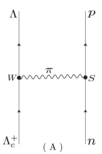
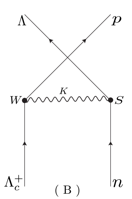
Figure 1: One meson exchange diagrams for tree-level processes involving $\Lambda^{+}_{c}n$ interaction. The diagram $(A)$ corresponds to the one-pion exchange contribution and the diagram $(B)$ corresponds to the one-kaon exchange contribution for the two-body transition amplitude.

For the NMWD dynamics we adopt the one-meson-exchange model (OME) including only the pion ($\pi$) and kaon ($K$) contributions. Therefore, the transition amplitude ${{\cal M}}$ for the two-body NMWD reaction in Eq. (4) can be obtained from the Feynman rules applied to the two diagrams in Fig. 1. Due to strangeness and charm selection rules, the $\pi$ meson contributes only to diagram (A) and the $K$ meson contributes only to diagram (B). The baryon-baryon-meson weak ($W$) and strong ($S$) vertices for $\pi$ and $K$ are taken from the corresponding coupling-Hamiltonians, which are:

1. For one-pion-exchange:

   $$\mathcal{H}^{S}_{NN\pi} = ig_{NN\pi}\bar{\Psi}_{N}\gamma_{5}\bm{\tau}\cdot\bm{\Phi}_{\pi}\Psi_{N},$$

   $$\mathcal{H}^{W}_{\Lambda_{c}\Lambda\pi} = iG_{F}\,m_{\pi}^{2}\bar{\Psi}_{\Lambda}\left(\,A_{\pi}+B_{\pi}\gamma_{5}\,\right)\bm{\tau}\cdot\bm{\Phi}_{\pi}\Psi_{\Lambda_{c}},$$ (13)

   where $\bm{\tau}$ is the isospin operator, $\bm{\Phi}_{\pi}$ and $\Psi_{N}$ are pion and nucleon fields, and $A_{\pi}$ and $B_{\pi}$ are parity-conserving (PC) and parity-violating (PV) amplitudes. The strange and charmed baryon fields are written in accordance with the isospurion strategy to enforce charge conservation in the vertices of Fig. 1, that is,

   $$\Psi_{\Lambda}=\psi_{\Lambda}\left(\negthinspace\begin{array}[]{c}0\\ 1\end{array}\right),\hskip 2.84544pt\Psi_{\Lambda_{c}}=\psi_{\Lambda^{+}_{c}}\left(\negthinspace\begin{array}[]{c}1\\ 0\end{array}\right).$$ (14)

   The strong coupling constant is $g_{NN\pi}=13.3$ and the Fermi coupling constant is given by $G_{F}m_{\pi}^{2}=2.21\times 10^{-7}$. We use the experimental values from the CLEO collaboration [73] for the PC and PV amplitudes: $A_{\pi}=-1.56$ and $B_{\pi}=6.63$ — note that these values are in units of $G_{F}m^{2}_{\pi}$, while the CLEO collaboration quotes the results is units of $G_{F}V_{cs}V_{ud}\times 10^{-2}~{}{\rm GeV}^{2}$, where $V_{cs}$ and $V_{ud}$ are the standard Cabbibo-Maskawa-Kobayashi matrix elements.

2. For one-kaon-exchange:

   $$\mathcal{H}^{S}_{N\Lambda K} = ig_{N\Lambda K}\,\bar{\psi}_{\Lambda}\gamma_{5}\ (\,\Phi^{(K)}\,)^{\dagger}\Psi_{N},$$

   $$\mathcal{H}^{W}_{\Lambda_{c}NK} = iG_{F}\,m_{\pi}^{2}\bar{\psi}_{p}\left(\,A_{K}+B_{K}\gamma_{5}\right)\phi^{(K^{0})}\psi_{\Lambda^{+}_{c}},$$ (15)

   where $\psi_{\Lambda^{+}_{c}}$ and $\psi_{p}$ are the charmed and proton fields, $A_{K}$ and $B_{K}$ are the PC and PV amplitudes, respectively. For kaons we can write the field operator $\Phi^{(K)}$ and its hermitian conjugate $(\,\Phi^{(K)}\,)^{\dagger}$ as

   $$\Phi^{(K)} = \left(\negthinspace\begin{array}[]{c}\phi^{(K^{+})}\\ \phi^{(K^{0})}\end{array}\right),\hskip 5.69046pt(\,\Phi^{(K)}\,)^{\dagger}=\left(\negthinspace\begin{array}[]{cc}\phi^{(K^{+})^{\dagger}}&\phi^{(K^{0})^{\dagger}}\end{array}\right).$$ (19)

   The strong coupling-constant is $g_{N\Lambda K}=-14.1$. There are no experimental values for the PV and PC amplitudes $A_{K}$ and $B_{K}$; we use the values from theoretical predictions in Ref. [74] for the $\Lambda^{+}_{c}\rightarrow p+\bar{K}^{0}$ weak transition, namely $A_{K}=-0.95$ and $B_{K}=9.17$, in units of $G_{F}m^{2}_{\pi}$.

When applying the Feynman rules, the baryon field operators should be expanded in terms of the eigenfunctions of the corresponding single-particle Hamiltonians in Eq. (11). Doing this, one gets for the two-body transition amplitude

$${{\cal M}}({\bf p}_{\Lambda}s_{\Lambda},{\bf p}_{p}s_{p};j_{\Lambda^{+}_{c}}m_{\Lambda^{+}_{c}},j_{n}m_{n})={{\cal M}}^{\pi}-{{\cal M}}^{K},$$ (20)

with

$${{\cal M}}^{\pi} = \int d{\bf x}\,d{\bf y}\,\bar{\psi}_{\mathbf{p}_{\Lambda}s_{\Lambda}}(\mathbf{x})\Gamma^{\pi}(t_{\Lambda},t_{p})\Psi_{j_{\Lambda^{+}_{c}}m_{\Lambda^{+}_{c}}}(\mathbf{x})\Delta^{\pi}(|\mathbf{x}-\mathbf{y}|)\bar{\psi}_{\mathbf{p}_{p}s_{p}}(\mathbf{y})\gamma_{5}\Psi_{j_{n}m_{n}}(\mathbf{y}),$$

$${{\cal M}}^{K} = \int d{\bf x}\,d{\bf y}\,\bar{\psi}_{\mathbf{p}_{p}s_{p}}(\mathbf{x})\Gamma^{K}(t_{p},t_{\Lambda})\Psi_{j_{\Lambda^{+}_{c}}m_{\Lambda^{+}_{c}}}(\mathbf{x})\Delta^{K}(|\mathbf{x}-\mathbf{y}|)\bar{\psi}_{\mathbf{p}_{\Lambda}s_{\Lambda}}(\mathbf{y})\gamma_{5}\Psi_{j_{n}m_{n}}(\mathbf{y}),$$ (21)

where the negative sign in Eq. (20) comes from the crossing of two fermion lines in Fig. 1(B). The baryon bound and free Dirac wave-functions $\Psi$ and $\psi$ , respectively, have the forms given in Eqs. (54) and (59)–(61), and we have defined matrices

$$\Gamma^{\pi}(t_{\Lambda},t_{p}) = {{\cal A}}^{\pi}(t_{\Lambda},t_{p})+{{\cal B}}^{\pi}(t_{\Lambda},t_{p})\gamma_{5},$$

$$\Gamma^{K}(t_{p},t_{\Lambda}) = {{\cal A}}^{K}(t_{p},t_{\Lambda})+{{\cal B}}^{K}(t_{p},t_{\Lambda})\gamma_{5},$$ (22)

with the pion and kaon effective PC and PV coupling-constants given by

$${{\cal A}}^{\pi}(t_{\Lambda},t_{p}) = G_{F}m_{\pi}^{2}g_{\pi NN}A_{\pi}I(t_{\Lambda},t_{p}),\hskip 5.69046pt{{\cal B}}^{\pi}(t_{\Lambda},t_{p})=G_{F}m_{\pi}^{2}g_{\pi NN}B_{\pi}I(t_{\Lambda},t_{p}),$$

$${{\cal A}}^{K}(t_{p},t_{\Lambda}) = G_{F}m_{\pi}^{2}g_{K\Lambda N}A_{K}K(t_{p},t_{\Lambda}),\hskip 5.69046pt{{\cal B}}^{K}(t_{p},t_{\Lambda})=G_{F}m_{\pi}^{2}g_{K\Lambda N}B_{K}K(t_{p},t_{\Lambda}),$$ (23)

where $I(t_{\Lambda},t_{p})=2$ and $K(t_{p},t_{\Lambda})=1$ are isospin factors.

For the meson propagators, we attach at each vertex the form factor

$$F_{M}(q^{2})=\frac{\Lambda_{M}^{2}-m_{M}^{2}}{\Lambda_{M}^{2}+q^{2}},$$

with $q^{2}\equiv(q^{0})^{2}-\bm{q}^{2}$, where $q$ is the transferred momentum, getting

$$\mathsf{\Delta}^{M}(|\mathbf{x}-\mathbf{y}|)=\int\,\frac{d{\bf q}}{(2\pi)^{3}}\,\frac{e^{-i\mathbf{q}\cdot(\mathbf{x}-\mathbf{y})}}{(q^{0})^{2}-\mathbf{q}^{2}-m_{M}^{2}+i\varepsilon}\,F_{M}^{2}\left(\,(q^{0})^{2}-\mathbf{q}^{2}\,\right),$$ (24)

for $M=\pi,K$. These propagators depend on the energy $q^{0}$ carried by the exchanged meson, which is taken as $q^{0}=(q_{W}^{0}+q_{S}^{0})/2$, with $q_{W}^{0}$ and $q_{S}^{0}$ fixed by energy conservation at the weak ($W$) and strong ($S$) vertices. The numerical values for the cutoffs are the same as those used in Ref. [58], namely, $\Lambda_{\pi}=1.3$ GeV and $\Lambda_{K}=1.2$ GeV.

To conclude this section, we mention that the angular integrations in the transition amplitude in Eq. (20) can be simplified by performing partial-wave expansions. This is done in B.

4 Decay rate

The NMWD rate of a single-$\Lambda^{+}_{c}$ charmed nucleus of baryon number $A$ in its ground state with spin $J_{I}$ and spin-projection $M_{I}$ and energy $E_{I}$, i.e., the partial width for its decay through the reaction in Eq. (4) into a residual nucleus with $(A-2)$ nucleons, emitting a $\Lambda$-hyperon and a proton, is given by the Fermi Golden Rule as

$$\Gamma_{nm} = \frac{2\pi}{\hat{J}^{2}_{I}}\sum_{M_{I}J_{F}M_{F}\atop s_{\Lambda}s_{p}j_{n}}\int\left|{{\cal M}}_{A}({\bf p}_{\Lambda}{s_{\Lambda}},{\bf p}_{p}{s_{p}},j_{n}J_{F}M_{F};J_{I}M_{I})\right|^{2}$$ (25)

$$\times \delta(E_{I}-E_{F}-T_{R}-E_{\Lambda}-E_{p})\frac{d{\bf p}_{\Lambda}}{(2\pi)^{3}}\frac{d{\bf p}_{p}}{(2\pi)^{3}},$$

where ${{\cal M}}_{A}$ is the relativistic nuclear transition amplitude that is specified below, $E_{F}$ and $j_{n}J_{F}M_{F}$ ($j\equiv(nlj)$) are the energy and quantum numbers of the final states of the residual nucleus (cf. Eq. (7)). In addition, ($E_{p},{\bf p}_{p},s_{p}$) and ($E_{\Lambda},{\bf p}_{\Lambda},s_{\Lambda}$) are energies, momenta and spin projections of outgoing $p$ and $\Lambda$. There is no summation over isospin projections in Eq. (25) since they have fixed values in the NMWD process in Eq. (4), namely $t_{p}=1/2$ and $t_{\Lambda}=-1/2$. We have included in the energy conservation condition the recoil energy

$$T_{R}\equiv T_{R}(\cos\theta_{\Lambda p})=\sqrt{M_{R}^{2}+p_{\Lambda}^{2}+p_{p}^{2}+2p_{\Lambda}\,p_{p}\cos\theta_{\Lambda p}}-M_{R},$$ (26)

where $M_{R}\approx(A-2)M_{N}$ is the mass of the residual nucleus and $\theta_{\Lambda p}$ is the angle between the two outgoing particles.

Within the IPSM, the relations in Eqs. (5) and (7) allow us to write

$$E_{I} = E_{C}+\varepsilon_{j_{\Lambda^{+}_{c}}}+M_{\Lambda^{+}_{c}},$$

$$E_{F} = E_{C}-\varepsilon_{j_{n}}-M_{N},$$ (27)

where $E_{C}$ is the energy of the core. Thus, the argument of the energy-conserving delta-function in Eq. (25) reads

$$E_{I}-E_{F}-T_{R}-E_{\Lambda}-E_{p}=\Delta_{j_{n}}-T_{\Lambda}-T_{p}-T_{R},$$ (28)

where

$$T_{i}=E_{i}-M_{i}\quad\quad(i=\Lambda,p),$$ (29)

are kinetic energies, and

$$\Delta_{j_{n}}=\Delta_{c}+\varepsilon_{j_{\Lambda^{+}_{c}}}+\varepsilon_{j_{n}},$$ (30)

is the liberated energy. Moreover, from

$$p_{i}=\sqrt{T_{i}\,(T_{i}+2M_{i})\,}\quad\quad(\,i=\Lambda,p\,),$$ (31)

one gets

$$d{\bf p}_{i}={p}_{i}^{2}\,dp_{i}\,d\hat{\bf p}_{i}=(M_{i}+T_{i})\,\sqrt{T_{i}\,(2M_{i}+T_{i})}\,dT_{i}\,d\hat{\bf p}_{i},\quad\quad(i=\Lambda,p),$$ (32)

which gives

$$\Gamma_{nm}=2\pi\,\int\,\frac{dT_{\Lambda}}{(2\pi)^{3}}\,\frac{dT_{p}}{(2\pi)^{3}}\,\rho(T_{\Lambda},T_{p})\mathcal{I}(p_{\Lambda},p_{p}),$$ (33)

where

$$\rho(T_{\Lambda},T_{p})=(\mathrm{M}_{\Lambda}+T_{\Lambda})\,\sqrt{T_{\Lambda}\,(2\,\mathrm{M}_{\Lambda}+T_{\Lambda})}\,(\mathrm{M}_{p}+T_{p})\sqrt{T_{p}\,(2\,\mathrm{M}_{p}+T_{p})},$$ (34)

and

$$\mathcal{I}(p_{\Lambda},p_{p}) = \hat{J}^{-2}_{I}\sum_{M_{I}J_{F}M_{F}\atop s_{\Lambda}s_{p}j_{n}}\int d\hat{\bf p}_{{\Lambda}}\,d\hat{\bf p}_{p}\,\left|{{\cal M}}_{A}({\bf p}_{\Lambda}{s_{\Lambda}},{\bf p}_{p}{s_{p}},j_{n}J_{F}M_{F};J_{I}M_{I})\right|^{2}$$ (35)

$$\times \delta(\Delta_{j_{n}}-T_{\Lambda}-T_{p}-T_{R}).$$

To conduct the discussion as simply as possible, we will start with charmed hypernuclei having a doubly-closed-subshell core (DCSC). In this case, $J_{C}=0$, and from Eq. (7), the IPSM yields $J_{I}=j_{\Lambda^{+}_{c}}$, $M_{I}=m_{\Lambda^{+}_{c}}$, $J_{F}=j_{n}$, and $M_{F}=m_{n}$. Furthermore, noticing that, in the IPSM, such a core functions as the vacuum, $|\underline{0}\rangle$, for particles, anti-particles and holes, Eqs. (5)-(7) take the form

$$|J_{C}\rangle = |\underline{0}\rangle,$$ (36)

$$|J_{I}\rangle = a^{\dagger}_{j_{\Lambda^{+}_{c}}}|\underline{0}\rangle,$$ (37)

$$|J_{F}\rangle = \tilde{a}_{j_{n}}|\underline{0}\rangle,$$ (38)

which imply that the DCSC nuclear transition amplitude ${{\cal M}}_{A}$ is, except for an irrelevant phase-factor, just the two-body transition amplitude ${{\cal M}}$ described in Section 3. Therefore, Eq. (35) gives

$$\mathcal{I}^{\mathrm{DCSC}}(p_{\Lambda},p_{p}) = \hat{j}_{\Lambda^{+}_{c}}^{-2}\sum_{m_{\Lambda^{+}_{c}}j_{n}m_{n}}\sum_{{s_{\Lambda}}{s_{p}}}\int d\hat{\bf p}_{{\Lambda}}d\hat{\bf p}_{p}\,|{{\cal M}}({\bf p}_{\Lambda}s_{\Lambda},{\bf p}_{p}s_{p};j_{\Lambda^{+}_{c}}m_{\Lambda^{+}_{c}},j_{n}m_{n})|^{2}$$ (39)

$$\times \delta(\Delta_{j_{n}}-T_{\Lambda}-T_{p}-T_{R}).$$

When nuclear recoil is neglected, i.e. setting $T_{R}=0$, we can use the completeness relation in Eq. (64) to integrate over angles in Eq. (39), getting

$$\mathcal{I}^{\mathrm{DCSC}}(p_{\Lambda},p_{p})=\frac{(4\pi)^{4}}{\hat{j}_{\Lambda^{+}_{c}}^{2}}\sum_{\kappa_{\Lambda}\kappa_{p}j_{n}J}(2J+1)\left|{\sf M}_{J}\right|^{2}\delta(\Delta_{j_{n}}-T_{\Lambda}-T_{p})\qquad\mbox{(no recoil)},$$ (40)

where

$${\sf M}_{J}={\sf M}^{\pi}_{J}-(-)^{j_{\Lambda}+j_{p}+J}{\sf M}^{K}_{J},$$ (41)

is the total angular-momentum-coupled matrix element, the definition and meaning of which were explained in B. In obtaining this result, we have eliminated the Clebsh-Gordan coefficients that appear in Eq. (68) by performing summations on angular momentum projections.

Thus, from Eq. (33), after integrating on $T_{p}$, we get that, for a DCSC charmed hypernucleus, when described by the IPSM, the NMWD rate reads

$$\Gamma_{nm}^{\mathrm{DCSC}}=\frac{8}{\pi}\sum_{\kappa_{\Lambda}\kappa_{p}j_{n}J}\frac{\hat{J}^{2}}{\hat{j}_{\Lambda^{+}_{c}}^{2}}\int_{0}^{\Delta_{j_{n}}}dT_{\Lambda}\left[\rho(T_{\Lambda},T_{p})\left|{\sf M}_{J}\right|^{2}\right]_{T_{p}=\Delta_{j_{n}}-T_{\Lambda}}\qquad\mbox{(no recoil)},$$ (42)

with ${\sf M}_{J}$ given by Eq. (41) (for the $\pi+K$ OME model).

From previous works of Refs. [54, 55, 58, 65, 75, 76], we know that to describe the NMWD in $\Lambda$ hypernuclei with open-shell cores within the IPSM it is enough to make the replacement $\hat{J}^{2}/\hat{j}^{2}_{\Lambda}\rightarrow F^{j_{N}}_{J}$ in the decay-rate expression with the DCSC, where $F^{j_{N}}_{J}$ is a spectroscopic factor. Making the same replacements here, i.e. $\hat{J}^{2}/\hat{j}^{2}_{\Lambda^{+}_{c}}\rightarrow F^{j_{N}}_{J}$ in Eq. (42), with $F^{j_{N}}_{J}$ given by Eq. (10), we get that NMWD rate in recoilless charmed hypernuclei is given by

$$\Gamma_{nm} = \frac{8}{\pi}\sum_{\kappa_{\Lambda}\kappa_{p}j_{n}J}F^{j_{n}}_{J}\int_{0}^{\Delta_{j_{n}}}dT_{\Lambda}dT_{p}\,\rho(T_{\Lambda},T_{p})\left|{\sf M}_{J}\right|^{2}\delta(\Delta_{j_{n}}-T_{\Lambda}-T_{p}),$$ (43)

$$= \frac{8}{\pi}\sum_{\kappa_{\Lambda}\kappa_{p}j_{n}J}F^{j_{n}}_{J}\int_{0}^{\Delta_{j_{n}}}dT_{\Lambda}\left[\rho(T_{\Lambda},T_{p})\left|{\sf M}_{J}\right|^{2}\right]_{T_{p}=\Delta_{j_{n}}-T_{\Lambda}}\hskip 5.69046pt\mbox{(no recoil)},$$

for both open- and closed-subshell cores.

5 Effect of nuclear recoil

When including recoil, one needs to perform the angular integration in Eq. (35). We proceed as indicated in Eqs. (55)-(57) of Ref. [58], in that one makes the replacement

$$\int dT_{\Lambda}dT_{p}\delta(\Delta_{j_{n}}-T_{\Lambda}-T_{p})\rightarrow\frac{1}{2}\int d\cos\theta_{\Lambda p}dT_{\Lambda}dT_{p}\,\delta(\Delta_{j_{n}}-T_{\Lambda}-T_{p}-T_{R})\,\cdots,$$ (44)

in the first branch of Eq. (43), getting

$$\Gamma_{nm}=\frac{4}{\pi}\sum_{\kappa_{\Lambda}\kappa_{p\,}j_{n}J}F^{j_{n}}_{J}\,\int\,d\cos\theta_{\Lambda p}\,dT_{\Lambda}\,dT_{p}\,\rho(T_{\Lambda},T_{p})\,\left|{\sf M}_{J}\right|^{2}\,\delta[f(T_{p})],$$ (45)

where $f(T_{p})$ is given by

$$f(T_{p})=\Delta_{j_{n}}-T_{\Lambda}-T_{p}-T_{R}.$$ (46)

Details on the evaluation of the integration over $T_{p}$ are presented in C. The final result for the rate can be expressed as

$$\Gamma_{nm} = \frac{4}{\pi}\sum_{\kappa_{\Lambda}\kappa_{p}j_{n}J}\,F^{j_{n}}_{J}\,\int dT_{\Lambda}\,\int d\cos\theta_{\Lambda p}\,\theta(K_{2})$$ (47)

$$\times \left\{\left[\,\frac{\rho(T_{\Lambda},T_{p})}{|f^{\prime}(T_{p})|}\theta(T_{p})\,\theta_{0}[f(T_{p})]\,\left|{\sf M}_{J}\right|^{2}\right]_{T_{p}\to T_{p}^{+}}+\left[\;\cdot\;\right]_{T_{p}\to T_{p}^{-}}\right\},$$

where $T^{\pm}_{p}$ is given by

$$T_{p}^{\pm} = \frac{K_{1}(T_{\Lambda},\cos\theta_{\Lambda p})\pm|p_{\Lambda}\cos\theta_{\Lambda p}|\sqrt{K_{2}(T_{\Lambda},\cos\theta_{\Lambda p}})}{2K_{3}(T_{\Lambda},\cos\theta_{\Lambda p})},$$ (48)

where $K_{1}$, $K_{2}$ and $K_{3}$ are given by Eqs. (105)-(107). Here, the step functions ensure positivity of $K_{2}$ and $T_{p}$, and $\theta_{0}(x)$

$$\theta_{0}(x)=\left\{\begin{array}[]{ll}1&\mbox{if}\;|x|<\epsilon\\ 0&\mbox{otherwise},\end{array}\right.$$ (49)

with $\epsilon$ being a suitably chosen small positive value, ensures that the roots are not spurious solutions to $f(T_{p})=0$ — see C for details. The intervals of integration in Eq. (47) are $-1<\cos\theta_{\Lambda p}<1$ and $0<T_{\Lambda}<T_{\Lambda}^{\mathrm{max}}$ with

$$T_{\Lambda}^{\mathrm{max}}=\frac{(2M_{p}+\Delta_{j_{n}})\Delta_{j_{n}}}{2(M_{p}+M_{\Lambda}+\Delta_{j_{n}})}\approx\frac{(2M_{p}+\Delta_{c})\Delta_{c}}{2(M_{p}+M_{\Lambda}+\Delta_{c})}=553\,\text{MeV}.$$ (50)

In what follows, we shall make reference to the $\Lambda$ kinetic energy spectrum and to the pair opening-angle distribution, which are, respectively, the partial integrands in the variables $T_{\Lambda}$ and $\cos\theta_{\Lambda p}$ and are denoted by

$$S(T_{\Lambda})=\frac{d\Gamma_{nm}}{dT_{\Lambda}},$$ (51)

and

$$S(\cos\theta_{\Lambda p})=\frac{d\Gamma_{nm}}{d\cos\theta_{\Lambda p}}.$$ (52)

6 Numerical Results and Discussion

We start presenting numerical results for the rate of the one-neutron-induced NMWD of ${}_{\Lambda^{+}_{c}}^{12}$N. We concentrate on this particular nucleus to compare results with the study of the ${}_{\Lambda}^{12}$C hypernucleus we have performed in Ref. [58]. As discussed in the previous sections, we employ the IPSM and consider the $\pi$ and $\pi+K$ OME model for the weak decay process. In this model, the neutron states contributing to the transition are the $j_{n}=1s_{1/2}$ and $1p_{3/2}$, and the $\Lambda^{+}_{c}$ is always considered to be in the state $j_{\Lambda^{+}_{c}}=1s_{1/2}$.

We remark that we have found numerically that the contribution from second term in Eq. (47), coming from the root $T_{p}=T^{-}_{p}$, is relatively small and may be neglected for all practical purposes. This same feature was seen in the nonrelativistic treatment of the recoil effect in the NMWD of the ${}_{\Lambda}^{12}$N hypernucleus; specifically, Eq. (63) of Ref. [58]. Here and there, this feature can be attributed to phase-space.

Table 1: Parity-conserving (PC), parity-violating (PV), and total decay rates for the nonmesonic weak decay ${}^{12}_{\Lambda^{+}_{c}}{\rm N}\rightarrow{{}^{10}{\rm C}}+p+\Lambda$, in units of $10^{-11}\text{MeV}$. Three approaches to recoil effects and two choices of OME models are considered.

Model	$\Gamma^{\text{PC}}_{nm}$	$\Gamma^{\text{PV}}_{nm}$	$\Gamma_{nm}$
No Recoil
$\pi\hskip 28.45274pt$	$1.31$	$0.89$	$2.20$
$\pi+K\hskip 2.84544pt$	$1.94$	$0.90$	$2.84$
Relativistic Recoil
$\pi\hskip 28.45274pt$	$0.91$	$0.59$	$1.50$
$\pi+K\hskip 2.84544pt$	$1.47$	$0.60$	$2.07$
Nonrelativistic Recoil
$\pi\hskip 28.45274pt$	$1.01$	$0.68$	$1.70$
$\pi+K\hskip 2.84544pt$	$1.55$	$0.69$	$2.24$

In Table 1 we present the different contributions to the rates. We consider separately contributions coming from the parity-conserving ($\Gamma^{\text{P}C}_{nm}$) and parity-violating ($\Gamma^{\text{P}V}_{nm}$) transitions, that correspond, respectively, to the $B$ and $A$ terms in Eqs. (13) and (15), and also give the total rate, $\Gamma_{nm}=\Gamma^{\text{P}C}_{nm}+\Gamma^{\text{P}V}_{nm}$, all of them are in units of $10^{-11}\text{MeV}$. We recall that the PC contribution to $\Gamma_{nm}$ comes from the amplitudes ${\cal A}^{\pi}$ and ${\cal A}^{K}$ and the PV contribution comes from ${\cal B}^{\pi}$ and ${\cal B}^{K}$, defined in Eq. (23). For each of these quantities we present three different sorts of results: first, results for the decay rates without recoil effects, computed with Eq. (43); second, results with relativistic recoil effects, computed with Eq. (47); and, finally, results with nonrelativistic recoil effects, in which a nonrelativistic approximation is made for the recoil energy $T_{R}$, following the procedure in Ref. [58] for the ${}_{\Lambda}^{12}$C hypernucleus.

The following conclusions can be drawn from the results displayed in the Table:

1. The contribution of the one kaon exchange potential is quite significant for the PC decay rate, but it is very small for the PV decay.

2. Recoil has a sizable impact on the rate and goes in the direction of decreasing it, at the level of 20% to 30%.

3. The difference between the results with relativistic and nonrelativistic treatment of recoil effects are at the level of 10%, surprisingly not a large effect.

4. The predicted NMWD rates $\Gamma_{nm}$ are of the same order of magnitude as the partial decay rate for the corresponding mesonic decay $\Gamma(\Lambda^{+}_{c}\rightarrow\Lambda+\pi)=(4.28\pm 0.26)\times 10^{-11}$ MeV, whose measured branching fraction, calibrated relative to the $pK^{-}\pi^{+}$ mode, is $B(\Lambda_{c}^{+}\to\Lambda+\pi^{+})=(1.07\pm 0.28)\%$ [35]. In Ref.  [73], is it reported the value $\Gamma(\Lambda^{+}_{c}\rightarrow\Lambda+\pi)=(0.40\pm 0.11)\times 10^{11}\rm{s}^{-1}=(2.63\pm 0.72)\times 10^{-11}\rm{MeV}$.

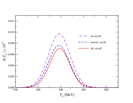
Figure 2: The ${}_{\Lambda^{+}_{c}}^{12}$N NMWD spectrum as a function of the kinetic energy $T_{\Lambda}$, evaluated without recoil (dash-dotted violet-line), with nonrelativistic recoil (dashed blue-line) and with relativistic recoil (solid red-line).

In Fig. 2 we show the $\Lambda$ kinetic energy spectrum $S(T_{\Lambda})$, defined in Eq. (51). The figure shows the spectra evaluated without recoil, with fully relativistic recoil and with nonrelativistic recoil. Independently of how the recoil effect is treated, the kinetic energy spectra $S(T_{\Lambda})$ always have a symmetric bell shape, with centroid at about $T_{\Lambda}=300$ MeV, which is roughly half the maximum energy $T_{\Lambda}^{\mathrm{max}}$ of the emitted $\Lambda$.

Finally, in Fig. 3 we show the results for the opening-angle distribution $S(\cos\theta_{\Lambda p})$, defined in Eq. (52). We recall that the angular distribution of the emitted particles is due to recoil; when recoil is neglected, the particles are emitted back to back. We show results calculated with relativistic and nonrelativistic expressions for the recoil. The opening-angle distribution $S(\cos\theta_{\Lambda p})$ in Fig. 3 is similar to the analogous one $S_{p}(\cos\theta_{np})$ of Fig. 2 in Ref. [76], in that it has a maximum for $\cos\theta_{\Lambda p}=-1$, but it extends a little further towards smaller angles.

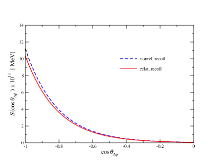
Figure 3: Opening-angle distribution of the emitted $\Lambda$-$p$ pair in the ${}_{\Lambda^{+}_{c}}^{12}$N NMWD, evaluated with nonrelativistic recoil (dashed blue-line) and with relativistic recoil (solid red-line).

7 Conclusions and Perspectives

The investigation of the production of heavy flavor hadrons containing a charm-quark and their interaction with ordinary hadrons in nuclear medium is of considerable contemporary interest once it provides an additional means for a better understanding of new forms of nuclear matter [4, 5]. A major difficulty in such an investigation program is the lack of experimental information on the free-space and in-medium interactions involving charmed hadrons unlike what happens in similar problems involving strange hadrons. In a situation with a lack of experimental information, one way to proceed in model building is to use symmetry constraints and analogies with other similar processes. With such a motivation, we investigated in this work the nonmesonic weak decay of nuclei containing a single $\Lambda_{c}^{+}$, relying on previous experience with the analogous $\Lambda$ hypernucleus.

We have discussed in Sections 2 and 3 the extension to the ${}^{12}_{\Lambda^{+}_{c}}{\rm N}$ hypernucleus of a relativistic formalism previously developed in Ref. [58] for the NMWD of the ${}^{12}_{\Lambda}{\rm C}$ hypernucleus. We have worked within the framework of the IPSM, with the dynamics of the $\Lambda^{+}_{c}n\to\Lambda p$ decay described by the $(\pi,K)$ OME model, with unknown couplings fixed by $SU(4)$ flavor symmetry. Dirac plane waves were expanded in spherical partial waves, meson propagators were multipole-expanded, so that the two-body transition matrix elements of the transition could be expressed in terms of two-dimensional radial integrals. Next, in Section 4, we have implemented the formalism for hypernuclei whose cores have only closed subshells. Then, to make contact with previous calculations, we have neglected nuclear recoil effects, which allowed us to reduce six-dimensional momentum-space integrals to simple one-dimensional integrals. The result obtained within this approximation was then generalized to include hypernuclei with open-shell cores. Finally, in Section 5, we have implemented a fully relativistic treatment of the recoil effects. Our results have shown that nuclear recoil has a sizable impact on the decay rate, and goes in the direction of decreasing it by 20% to 30%. Nuclear recoil gives an angular distribution to the emitted $\Lambda p$ pair and impacts significantly single kinetic energy spectra.

Very recently, the authors of Ref. [77] have suggested that small-sized (typically with $A=3$) charmed hypernuclei can be formed in nuclear collisions and identified through their mesonic decays [56] — in this respect, a recent exact three-body calculation [78] using baryon-baryon interactions obtained from a chiral constituent quark model predicts a $J=3/2$ charmed hypertriton with a binding energy between $140$ and $715$ MeV. Our study, on the other hand, suggests identification of the formation of charm hypernuclei via nonmesonic weak decays, which are unique, as they can only occur in the nucleus. Moreover, one of the the most interesting aspects of our results is that the predicted NMWD rate is of the same order of magnitude as the measured decay rate for the corresponding weak mesonic decay:

$$\Gamma_{nm}(^{12}_{\Lambda^{+}_{c}}{\rm N}\rightarrow{{}^{10}{\rm C}}+p+\Lambda)\simeq\Gamma(\Lambda_{c}^{+}\to\Lambda+\pi^{+}).$$ (53)

Branching ratios even smaller than $B(\Lambda_{c}^{+}\to\Lambda+\pi^{+})=(1.07\pm 0.28)\%$ have been measured [35]. This suggests that once the charmed hypernucleus ${}^{12}_{\Lambda^{+}_{c}}{\rm N}$ is produced, its NMWD should be measurable. We have limited our discussion to ${}^{12}_{\Lambda^{+}_{c}}{\rm N}$, but it is expected that the NMWD will be very similar in other $\Lambda_{c}$ hypernuclei, since this is the case in $\Lambda$ hypernuclei, as can be seen in Table II in Ref. [79]. This makes it even more feasible to detect the $\Lambda p$ pair in the final state. Needless to say that knowledge of kinetic energy spectra and of opening-angle $\Lambda p$ correlations such as those shown in Figs. 2 and 3 would be of help in this search. One should be aware, however, of the difficulties involved in the identification of a charmed nucleus like ${}^{12}_{\Lambda^{+}_{c}}{\rm N}$ in a $\bar{p}-$nucleus collision. One possibility would be the production through the reaction chain $\bar{p}+p\rightarrow D^{+}+D^{-}$, $D^{+}+^{12}\textrm{C}\rightarrow^{12}_{\Lambda^{+}_{c}}\textrm{N}+\pi^{0}$. The difficulty here is related to the detection of the $\pi^{0}$ in the final state. On the other hand, the direct process $\bar{p}+p\rightarrow\Lambda^{+}_{c}+\bar{\Lambda}^{-}_{c}$, as suggested in Ref. [17], would produce a proton hole in ${}^{12}\textrm{C}$, giving rise to the charmed hipernucleus with $A=12$ and $Z=6$, i.e. a ${}^{12}_{\Lambda^{+}_{c}}{\rm C}$ with six neutrons, five protons and one $\Lambda^{+}_{c}$. We reserve for a future publication the investigation of the NMWD of this nucleus.

To conclude, we mention that our study is a first incursion in the study of NMWD of charmed hypernuclei. We have limited the study to a two-body final state in the decay of $\Lambda^{+}_{c}$ but, of course, decay processes with larger branching ratios involving multiparticle final states should be explored in the identification of the formation and decay of charmed hypernuclei. Therefore, one can envisage a long path, both in theory and experiment, in the production of these fascinating new forms of nuclear matter.

Appendix A Bound and continuum single-particle wave functions

For completeness and to make the paper self-contained, we collect here the relevant formular associated with the bound and continuum single-particle wave functions. The bound single-particle wave functions have the general form

$$\Psi_{\kappa m}({\bf r})=\frac{1}{r}\left(\negthinspace\begin{array}[]{c}F_{\kappa}(r)\Phi_{\kappa m}(\hat{\bf r})\\ -iG_{\kappa}(r)\Phi_{-\kappa m}(\hat{\bf r})\end{array}\right)\equiv\left(\negthinspace\begin{array}[]{c}{}^{\uparrow}\Psi_{\kappa m}({\bf r})\\ -i^{\downarrow}\Psi_{\kappa m}({\bf r})\end{array}\right).$$ (54)

with $\kappa=\pm 1,\pm 2,\dots$, $j_{\kappa}=|\kappa|-1/2$,

$$l_{\kappa}=\left\{\begin{array}[]{ll}\kappa&\mbox{for $\kappa>0$,}\\ -\kappa-1&\mbox{for $\kappa<0$.}\end{array}\right.$$ (55)

The angular part is written, in standard notation, as

$$\Phi_{\kappa m}(\hat{\bf r})=\sum_{s\mu}(l\mu\frac{1}{2}s|jm)\,Y_{l\mu}(\hat{\bf r})\chi_{s}.$$ (56)

The radial part is determined from the eigenvalue equation

$$\hat{h}\,\Psi_{\kappa m}({\bf r})=(M+\varepsilon_{\kappa})\,\Psi_{\kappa m}({\bf r}),$$ (57)

where $\varepsilon_{\kappa}$ are the single-particle energies (s.p.e.), and the normalization is

$$\int d{\bf r}\;\Psi_{\kappa m}^{\dagger}({\bf r})\,\Psi_{\kappa m}({\bf r})=1.$$ (58)

Table 2: Single-particle energies obtained from the MFA for ${}^{12}{\rm C}$. For the experimental values for ${}^{12}\textrm{C}$, see the explanation in the text. The last line gives the ${1s}_{1/2}$ single-particle energy for the $\Lambda^{+}_{c}$ in ${}^{12}_{\Lambda^{+}_{c}}{\rm N}$ hypernucleus (composed by 6 protons, 5 neutrons and 1 $\Lambda^{+}_{c}$). All energies are in MeV.

Energy Level	Calculated	Experiment ${}^{12}\textrm{C}$
${\mbox{1s}_{1/2}}_{p}$	$-38.53$	$-33.5$
${\mbox{1p}_{3/2}}_{p}$	$-13.52$	$-15.96$
${\mbox{1s}_{1/2}}_{n}$	$-42.03$	$-36.3$
${\mbox{1p}_{3/2}}_{n}$	$-16.65$	$-18.72$
${\mbox{1s}_{1/2}}_{\Lambda^{+}_{c}}$   in   ${}^{12}_{\Lambda^{+}_{c}}\textrm{N}$	$-14.32$	$-$

Table 2 presents the results for the single-particle energies (s.p.e.) — the values of the parameters are fixed as discussed at the end of Sec. ISPM. The experimental values for neutron and proton $1p_{3/2}$ s.p.e. in ${}^{12}\textrm{C}$ are taken to be $\mbox{1p}_{3/2}$ hole states obtained from the separation energies calculated from the differences of experimental binding energies of ${}^{12}\textrm{C}$, ${}^{11}\textrm{C}$ and ${}^{12}\textrm{B}$ [80] : $\mathcal{B}(^{12}{\rm C})=92.16279$ MeV, $\mathcal{B}(^{11}{\rm C})=73.4414$ MeV, and $\mathcal{B}(^{11}{\rm B})=76.2059$ MeV. The proton $\mbox{1s}_{1/2}$ s.p.e. energy is obtained from data [81] on the knock-out reaction ¹²C(p,2p)¹¹B which indicate that the deep-proton-hole state $\mbox{1s}_{1/2}$ is located $\sim 20$ MeV above the $\mbox{1p}_{3/2}$ ground state in ¹¹B, giving a value of $\sim-33.5$ MeV for ${\mbox{1s}_{1/2}}_{p}$ in ${}^{12}{\rm C}$. However, knock-out reactions on neutrons such as (p,p’n) and (e,e’n) have not been reported, therefore, we assume that the energy separation between neutron $\mbox{1p}_{3/2}$ and $\mbox{1s}_{1/2}$ states is the same as that of the protons, which yields the value of $\sim-36.3$ MeV for the the ${\mbox{1s}_{1/2}}_{n}$ state (note that in our calculation of the s.p.e., the effect of the Coulomb force).

As remarked in Sec. 2, to describe the NMWD of ${}^{12}_{\Lambda_{c}^{+}}{\rm N}$ in the IPSM, the MFA is performed for ${}^{12}{\rm C}$, i.e. the $\Lambda^{+}_{c}$ wave functions should be those generated by mean fields for the ${}^{12}{\rm C}$ nucleus. However, it is instructive to estimate the effect of neglecting the contribution of $\Lambda^{+}_{c}$ to the sources of the meson mean fields. We have repeated the calculation of the bound wave functions by solving the Dirac and meson equations self-conistently, but still enforcing spherical symmetry of the nucleus. We found that the biding energies of the ${\mbox{1s}_{1/2}}_{p}$ and ${\mbox{1p}_{3/2}}_{p}$ states decrease by 10% and 20% respetively, of the $\Lambda^{+}_{c}$ is increased by 6%, and there is almost no change in the neutron binding energies. On the other hand, the changes in the bound-state wave functions lead o a change of the order of 1% in NMWD rates. Deviations from non-sphericity of the nuclei have not been estimated and their study is left for a future publication.

The continuum single-particle states should be taken as the positive-energy scattering eigenfunctions of the Hamiltonian in Eq. (11) with asymptotic momentum ${\bf p}$ and spin projection $s$. However, those will be approximated by the corresponding Dirac plane waves, which are expanded as follows (see Ref. [72], Appendix D):

$$\psi_{{\bf p}s}({\bf r})=\sum_{\kappa m}\langle\hat{\bf p}s|\kappa m\rangle^{\ast}\,\psi_{p\kappa m}({\bf r}),$$ (59)

with

$$\langle\hat{\bf p}s|\kappa m\rangle^{\ast}=4\pi i^{l}\sum_{\mu}(l\mu\frac{1}{2}s|jm)Y^{*}_{l\mu}(\hat{\bf p}),$$ (60)

and

$$\psi_{p\kappa m}({\bf r})=\left(\negthinspace\begin{array}[]{c}f_{p\kappa}(r)\Phi_{\kappa m}(\hat{\bf r})\\ -ig_{p\kappa}(r)\Phi_{-\kappa m}(\hat{\bf r})\end{array}\right)\equiv\left(\negthinspace\begin{array}[]{c}{}^{\uparrow}\psi_{p\kappa m}({\bf r})\\ -i\,^{\downarrow}\psi_{p\kappa m}({\bf r})\end{array}\right),$$ (61)

where the radial partial-waves, in unitary normalization, are

$$f_{p\kappa}(r)=\sqrt{\frac{E+\mathrm{M}_{N}}{2E}}j_{l_{\kappa}}(pr),$$ (62)

and

$$g_{p\kappa}(r)=-\mathrm{sgn}(\kappa)\sqrt{\frac{E-\mathrm{M}_{N}}{2E}}j_{{\bar{l}}_{\kappa}}(pr),$$ (63)

with ${\bar{l}}_{\kappa}=l_{-\kappa}$. The expansion coefficients $\langle\hat{\bf p}s|\kappa m\rangle^{\ast}$ fulfill the following relations

$$\sum_{s}\int d\hat{\bf p}\,\langle\hat{\bf p}s|\kappa m\rangle^{\ast}\langle\hat{\bf p}s|\kappa^{\prime}m^{\prime}\rangle=(4\pi)^{2}\delta_{\kappa\kappa^{\prime}}\delta_{mm^{\prime}},$$ (64)

and

$$2\hat{j}^{2}\delta_{jj^{\prime}}\sum_{sm}\int d\hat{\bf p}\,\langle\hat{\bf p}s|\kappa m\rangle^{\ast}\langle\hat{\bf p}s|\kappa^{\prime}m\rangle\cdots=(4\pi)^{2}\delta_{\kappa\kappa^{\prime}}\int_{-1}^{1}d\cos\theta\cdots\quad\quad.$$ (65)

The first of these relations can be easily verified, while the second one is shown in Appendix A of Ref. [58].

Appendix B Partial-wave decomposition of ${\cal M}^{\pi}$ and ${\cal M}^{K}$

Using Eq. (59) for both outgoing particles, the transition amplitude in Eq. (20) becomes

$${{\cal M}}=\underset{\kappa_{p}m_{p}}{\underset{\kappa_{\Lambda}m_{\Lambda}}{\sum}}\langle\hat{\bf p}_{\Lambda}s_{\Lambda}|\kappa_{\Lambda}m_{\Lambda}\rangle\,\langle\hat{\bf p}_{p}s_{p}|\kappa_{p}m_{p}\rangle({\sf M}^{\pi}-{\sf M}^{K}),$$ (66)

where

$${\sf M}^{\pi} \equiv \int d{\bf x}d{\bf y}\bar{\psi}_{p_{\Lambda}\kappa_{\Lambda}m_{\Lambda}}({\bf x})\Gamma^{\pi}(t_{\Lambda},t_{p}){\Psi}_{j_{\Lambda^{+}_{c}}m_{\Lambda^{+}_{c}}}({\bf x}){\mathsf{\Delta}}^{\pi}(|{\bf x}-{\bf y}|)\bar{\psi}_{p_{p}\kappa_{p}m_{p}}({\bf y})\gamma_{5}{\Psi}_{j_{n}m_{n}}({\bf y}),$$

$${\sf M}^{K} \equiv \int d{\bf x}d{\bf y}\bar{\psi}_{p_{p}\kappa_{p}m_{p}}(\mathbf{x})\Gamma^{K}(t_{p},t_{\Lambda})\Psi_{j_{\Lambda^{+}_{c}}m_{\Lambda^{+}_{c}}}(\mathbf{x})\mathsf{\Delta}^{K}(|\mathbf{x}-\mathbf{y}|)\bar{\psi}_{p_{\Lambda}\kappa_{\Lambda}m_{\Lambda}}(\mathbf{y})\gamma_{5}\Psi_{j_{n}m_{n}}(\mathbf{y}).$$ (67)

Now we introduce the angular momentum couplings ${\bm{J}}={\bm{j}}_{\Lambda^{+}_{c}}+{\bm{j}}_{n}$ and ${\bm{J}}^{\prime}={\bm{j}}_{\Lambda}+{\bm{j}}_{p}$ in ${\sf M}^{\pi}$, and ${\bm{J}}={\bm{j}}_{\Lambda^{+}_{c}}+{\bm{j}}_{n}$ and ${\bm{J}}^{\prime}={\bm{j}}_{p}+{\bm{j}}_{\Lambda}$ in ${\sf M}^{K}$. As ${\mathsf{\Delta}}^{M}$ is rotationally invariant, it turns out that $J=J^{\prime}$, which leads to

$${\sf M}^{\pi}-{\sf M}^{K}=\sum_{JM}(j_{\Lambda}m_{\Lambda}j_{p}m_{p}|JM)\,(j_{\Lambda^{+}_{c}}m_{\Lambda^{+}_{c}}j_{n}m_{n}|JM)({\sf M}^{\pi}_{J}-(-)^{j_{\Lambda}+j_{p}+J}{\sf M}^{K}_{J}),$$ (68)

where the phase $(-)^{j_{\Lambda}+j_{p}+J}$ comes from the property of Clebsh-Gordan coefficients $(j_{p}m_{p}j_{\Lambda}m_{\Lambda}|JM)=(-)^{j_{\Lambda}+j_{p}+J}(j_{\Lambda}m_{\Lambda}j_{p}m_{p}|JM)$. In more detail, one has for the pion contribution

$${\sf M}^{\pi}_{J} = -i\int d{\bf x}\,d{\bf y}{\mathsf{\Delta}}^{\pi}(|{\bf x}-{\bf y}|)\left\{\left[{{\cal A}}^{\pi}(t_{\Lambda},t_{p})\rho_{A}({\bf x})-i{{\cal B}}^{\pi}(t_{\Lambda},t_{p})\rho_{B}({\bf x})\right]\rho_{C}({\bf y})\right\}_{(J)},$$ (69)

where $(J)\equiv{(j_{\Lambda}j_{p},j_{\Lambda^{+}_{c}}j_{n};J)}$ indicates the angular momentum coupling described above, and the transition densities are

$$\rho_{A}({\bf x}) = {{}^{\uparrow}\psi}^{*}_{p_{\Lambda}\kappa_{\Lambda}}({\bf x}){{{}^{\uparrow}\Psi}_{\kappa_{\Lambda^{+}_{c}}}}({\bf x})-{{}^{\downarrow}\psi}^{*}_{p_{\Lambda}\kappa_{\Lambda}}({\bf x}){{{}^{\downarrow}\Psi}_{\kappa_{\Lambda^{+}_{c}}}}({\bf x}),$$

$$\rho_{B}({\bf x}) = {{}^{\uparrow}\psi}^{*}_{p_{\Lambda}\kappa_{\Lambda}}({\bf x}){{{}^{\downarrow}\Psi}_{\kappa_{\Lambda^{+}_{c}}}}({\bf x})+{{}^{\downarrow}\psi}^{*}_{p_{\Lambda}\kappa_{\Lambda}}({\bf x}){{{}^{\uparrow}\Psi}_{\kappa_{\Lambda^{+}_{c}}}}({\bf x}),$$

$$\rho_{C}({\bf y}) = {{}^{\uparrow}\psi}^{*}_{p_{p}\kappa_{p}}({\bf y}){{{}^{\downarrow}\Psi}_{\kappa_{n}}}({\bf y})+{{}^{\downarrow}\psi}^{*}_{p_{p}\kappa_{p}}({\bf y}){{{}^{\uparrow}\Psi}_{\kappa_{n}}}({\bf y}).$$ (70)

To carry out the coordinate integrations it is convenient to perform a tensor expansion of the propagators in Eq. (24), for $M=\pi,K$, as follows:

$${\mathsf{\Delta}}^{M}(|{\bf x}-{\bf y}|)=\sum_{L}{\mathsf{\Delta}}^{M}_{L}(x,y)\,[Y_{L}(\hat{\bf x})\cdot Y_{L}(\hat{\bf y})],$$ (71)

where $Y_{L}(\hat{\bf x})$ denotes the spherical tensor whose components are the spherical harmonics $Y_{LM}(\hat{\bf x})$ and similarly for $Y_{L}(\hat{\bf x})$, and

$${\mathsf{\Delta}}^{M}_{L}(x,y)=2\pi\int d(\cos\theta_{xy})\,{\mathsf{\Delta}}^{M}(|{\bf x}-{\bf y}|)\,P_{L}(\cos\theta_{xy}),$$ (72)

with $P_{L}$ being a Legendre polynomial. Thus, Eq. (69) becomes

$${\sf M}^{\pi}_{J} = -i\sum_{L}\int d{\bf x}\,d{\bf y}{\mathsf{\Delta}}^{\pi}_{L}(x,y)[Y_{L}(\hat{\bf x})\cdot Y_{L}(\hat{\bf y})]$$ (73)

$$\times \left\{\left[{{\cal A}}^{\pi}(t_{\Lambda},t_{p})\rho_{A}({\bf x})-i{{\cal B}}^{\pi}(t_{\Lambda},t_{p})\rho_{B}({\bf x})\right]\rho_{C}({\bf y})\right\}_{(J)},$$

Making use of the well known property of the scalar product of two tensor operators [82]

$$\langle j_{1}j_{2}J|[Y_{L}(\hat{\bf x})\cdot Y_{L}(\hat{\bf y})]|j_{3}j_{4}J\rangle\;=\;(-)^{j_{2}+j_{3}+J}\left\{\negthinspace\begin{array}[]{ccc}j_{1}&j_{2}&J\\ j_{4}&j_{3}&L\end{array}\right\}\langle j_{1}||Y_{L}||j_{3}\rangle\langle j_{2}||Y_{L}||j_{4}\rangle,$$ (74)

and defining

$$A^{L}_{\kappa\kappa_{\Lambda^{+}_{c}}}(rp) = [f_{p\kappa}(r)F_{\kappa_{\Lambda^{+}_{c}}}(r)-g_{p\kappa}(r)G_{\kappa_{\Lambda^{+}_{c}}}(r)]\,\langle\kappa||Y_{L}||\kappa_{\Lambda^{+}_{c}}\rangle,$$

$$B^{L}_{\kappa\kappa_{\Lambda^{+}_{c}}}(rp) = [f_{p\kappa}(r)G_{\kappa_{\Lambda^{+}_{c}}}(r)+g_{p\kappa}(r)F_{\kappa_{\Lambda^{+}_{c}}}(r)]\,\langle-\kappa||Y_{L}||\kappa_{\Lambda^{+}_{c}}\rangle,$$

$$C^{L}_{\kappa\kappa_{n}}(rp) = [f_{p\kappa}(r)G_{\kappa_{n}}(r)+g_{p\kappa}(r)F_{\kappa_{n}}(r)]\,\langle-\kappa||Y_{L}||\kappa_{n}\rangle,$$ (75)

a trivial, but tedious algebra gives

$${\sf M}_{J}^{\pi}=\sum_{L}(-)^{j_{p}+j_{{\Lambda^{+}_{c}}}+J}\left\{\negthinspace\begin{array}[]{ccc}j_{\Lambda}&j_{p}&J\\ j_{n}&j_{\Lambda^{+}_{c}}&L\end{array}\right\}{\sf M}_{L}^{\pi},$$ (76)

where

$${\sf M}_{L}^{\pi} \equiv -\int dxdy\,xy\;[{{\cal B}}^{\pi}(t_{\Lambda},t_{p})B^{L}_{\kappa_{\Lambda}\kappa_{\Lambda^{+}_{c}}}(xp_{\Lambda})+i{{\cal A}}^{\pi}(t_{\Lambda},t_{p})A^{L}_{\kappa_{\Lambda}\kappa_{\Lambda^{+}_{c}}}(xp_{\Lambda})]\,$$ (77)

$$\times {\mathsf{\Delta}}^{\pi}_{L}(x,y)\,C^{L}_{\kappa_{p}\kappa_{n}}(yp_{p}).$$

In the convention adopted in Eq. (56), the reduced matrix elements to be used in Eq. (75) are

$$\langle\kappa||Y_{L}||\kappa^{\prime}\rangle = (4\pi)^{-1/2}(-)^{l+l^{\prime}+j^{\prime}-1/2}\hat{j}\hat{j}^{\prime}\hat{L}\left(\negthinspace\begin{array}[]{ccc}j&L&j^{\prime}\\ -\frac{1}{2}&0&\frac{1}{2}\end{array}\right)\frac{1+(-)^{l+l^{\prime}+L}}{2},$$ (80)

$$\langle-\kappa||Y_{L}||\kappa^{\prime}\rangle = (4\pi)^{-1/2}(-)^{\bar{l}+l^{\prime}+j^{\prime}-1/2}\hat{j}\hat{j}^{\prime}\hat{L}\left(\negthinspace\begin{array}[]{ccc}j&L&j^{\prime}\\ -\frac{1}{2}&0&\frac{1}{2}\end{array}\right)\frac{1+(-)^{{\bar{l}}+l^{\prime}+L}}{2},$$ (83)

which satisfy the following symmetry property: $\langle\kappa||Y_{L}||{-\kappa^{\prime}}\rangle=\langle-\kappa||Y_{L}||\kappa^{\prime}\rangle$. The amplitude for the kaon contribution can be easily obtained by making the following substitutions in Eqs. (76) and (77): ${\sf M}_{J}^{\pi},{\sf M}_{L}^{\pi}\to{\sf M}_{J}^{K},{\sf M}_{L}^{K}$, $j_{\Lambda},\kappa_{\Lambda},p_{\Lambda}\leftrightarrow j_{p},\kappa_{p},p_{p}$, ${{\cal A}}^{\pi}(t_{\Lambda},t_{p}),{{\cal B}}^{\pi}(t_{\Lambda},t_{p})\rightarrow{{\cal A}}^{K}(t_{p},t_{\Lambda}),{{\cal B}}^{K}(t_{p},t_{\Lambda})$, and $\mathsf{\Delta}^{\pi},{\mathsf{\Delta}}^{\pi}_{L}\rightarrow\mathsf{\Delta}^{K},{\mathsf{\Delta}}^{K}_{L}$.

Appendix C Integration over $T_{p}$ in Eq. (45)

The first step towards the evaluation of the integration over $T_{p}$, we use Eq. (26) so that $f(T_{p})$ can be written as

$$f(T_{p})=a+T_{p}+\sqrt{b+T_{p}(c+T_{p})+d\,\sqrt{T_{p}(c+T_{p})}},$$ (84)

with

$$a=T_{\Lambda}-M_{R}-\Delta_{j_{n}},\hskip 5.69046ptb=M^{2}_{R}+p^{2}_{\Lambda},\hskip 5.69046ptc=2M_{p},\hskip 5.69046ptd=2p_{\Lambda}\cos\theta_{\Lambda p}.$$ (85)

We are then faced with an integration of the form

$$I=\int\,dx\,F(x)\,\delta[f(x)]$$ (86)

where $f(x)$ is defined in Eq. (84), with $x=T_{p}$:

$$f(x) = a+x+\sqrt{b+x(c+x)+d\,\sqrt{x(c+x)}},$$ (87)

and $a$, $b$, $c$ and $d$ defined in Eq. (85). To eliminate the delta-function, we use the identity

$$\delta[f(x)]=\sum_{n}\frac{\delta(x-x_{n})}{|f^{\prime}(x_{n})|},$$ (88)

where the summation is over all the real-valued simple zeros of $f(x)$, i.e.,

$$f(x_{n})=0,\hskip 5.69046ptf^{\prime}(x_{n})\neq 0.$$ (89)

Introducing 88 into Eq. 86 gives

$$I={\sum_{n}}^{\prime}\frac{F(x_{n})}{|f^{\prime}(x_{n})|},$$ (90)

where the prime in the summation sign is to remind that only those zeros that fall within the region of integration in Eq. 86 are to be included. In our case, $x$ stands for a kinetic energy, therefore we must require that $x_{n}>0$.

To find the zeros, we need to solve the equation $f(x)=0$, i.e.,

$$\sqrt{b+x(c+x)+d\,\sqrt{x(c+x)}} = -(a+x).$$ (91)

Squaring it, gives

$$d\,\sqrt{x(c+x)} = (a+x)^{2}-[b+x(c+x)],$$ (92)

and squaring this latter expression, gives

$$d^{2}\,x(c+x) = \{(a+x)^{2}-[b+x(c+x)]\}^{2}.$$ (93)

Noticing that

$$(a+x)^{2}-[b+x(c+x)]\equiv(a^{2}-b)-(c-2a)x,$$ (94)

it is clear that Eq. 93 can be written as

$$\alpha\,x^{2}+\beta\,x+\gamma = 0,$$ (95)

with the coefficients $\alpha,\beta,\gamma$ given in terms of $a,b,c,d$ as

$$\alpha = (c-2a)^{2}-d^{2},$$ (96)

$$\beta = -[2(a^{2}-b)(c-2a)+cd^{2}],$$ (97)

$$\gamma = (a^{2}-b)^{2}.$$ (98)

The roots of the quadratic equation 95 are given by

$$x^{\pm}_{n}=\frac{-\beta\pm\sqrt{\beta^{2}-4\alpha\gamma}}{2\alpha},$$ (99)

with the discriminant given by

$$\beta^{2}-4\alpha\gamma=d^{2}\{4(a^{2}-b)[(c-2a)c+(a^{2}-b)]+c^{2}d^{2}\}.$$ (100)

It is important to note that in the manipulations to arrive at Eq. 95, spurious solutions might have been introduced and one needs to verify whether these two roots do indeed satisfy the original equation, Eq. 91. Only then can they be taken as legitimate solutions to our problem. In particular, the derivative $f^{\prime}(x_{n})$ is given, at the legitimate zeros, by

$$f^{\prime}(x_{n})=1-\frac{c+2x_{n}}{2(a+x_{n})}-\frac{d(c+2x_{n})}{4(a+x_{n})\sqrt{x_{n}(c+x_{n})}}.$$ (101)

Since $x=T_{p}$ and $x^{\pm}=T^{\pm}_{p}$, one then have

$$\delta[f(T_{p})]=\frac{\delta(T_{p}-T_{p}^{+})}{|f^{\prime}(T^{+}_{p})|}+\frac{\delta(T_{p}-T_{p}^{-})}{|f^{\prime}(T^{-}_{p})|},$$ (102)

where

$$f^{\prime}(T^{\pm}_{p})=1-\frac{M_{p}+T^{\pm}_{p}}{T_{\Lambda}-M_{R}-\Delta_{j_{n}}+T^{\pm}_{p}}-\frac{p_{\Lambda}\cos\theta_{\Lambda p}(M_{p}+T^{\pm}_{p})}{(T_{\Lambda}-M_{R}-\Delta_{j_{n}}+T^{\pm}_{p})\sqrt{T^{\pm}_{p}(2M_{p}+T^{\pm}_{p})}},$$ (103)

with

$$T_{p}^{\pm} = \frac{K_{1}(T_{\Lambda},\cos\theta_{\Lambda p})\pm|p_{\Lambda}\cos\theta_{\Lambda p}|\sqrt{K_{2}(T_{\Lambda},\cos\theta_{\Lambda p}})}{2K_{3}(T_{\Lambda},\cos\theta_{\Lambda p})},$$ (104)

where

$$K_{1}(T_{\Lambda},\cos\theta_{\Lambda p}) = (M_{p}+M_{R}+\Delta_{j_{n}}-T_{\Lambda})\,[\Delta_{j_{n}}(2M_{R}+\Delta_{j_{n}})$$ (105)

$$- 2(M_{\Lambda}+M_{R}+\Delta_{j_{n}})T_{\Lambda}]$$

$$+ 2M_{p}\,T_{\Lambda}(2M_{\Lambda}+T_{\Lambda})\cos^{2}\theta_{\Lambda p},$$

$$K_{2}(T_{\Lambda},\cos\theta_{\Lambda p}) = [\Delta_{j_{n}}(2M_{R}+\Delta_{j_{n}})-2(M_{\Lambda}+M_{R}+\Delta_{j_{n}})T_{\Lambda}]$$ (106)

$$\times [4M_{p}(M_{p}+M_{R})+\Delta_{j_{n}}(2M_{R}+4M_{p}+\Delta_{j_{n}})$$

$$- 2(M_{\Lambda}+M_{R}+2M_{p}+\Delta_{j_{n}})T_{\Lambda}]$$

$$+ 4M_{p}^{2}\,T_{\Lambda}(2M_{\Lambda}+T_{\Lambda})\cos^{2}\theta_{\Lambda p},$$

$$K_{3}(T_{\Lambda},\cos\theta_{\Lambda p}) = (M_{p}+M_{R}+\Delta_{j_{n}}-T_{\Lambda})^{2}-T_{\Lambda}(2M_{\Lambda}+T_{\Lambda})\cos^{2}\theta_{\Lambda p}.$$ (107)

References

References

- [1] Choi S K et al. 2003 Phys. Rev. Lett. 91 262001
- [2] Lebed R F, Mitchell R E and Swanson E S 2017 Prog. Part. Nucl. Phys. 93 143
- [3] Krein G 2016 AIP Conf. Proc. 1701 020012
- [4] Briceño R A et al. 2016 Chin. Phys. C 40 042001
- [5] A. Hosaka A, Hyodo T, Sudoh K, Yamaguchi Y and Yasui S 2016 arXiv:1606.08685 [hep-ph]
- [6] Tsushima K, Lu D H, Thomas A W, Saito K and Landau R H 1999 Phys. Rev. C 59 2824
- [7] Yasui S and Sudoh K 2009 Phys. Rev. D 80 034008
- [8] Garcia-Recio C, Nieves J and Tolos L 2010 Phys. Lett. B 690 369
- [9] Garcia-Recio C, Nieves J, Salcedo LL and Tolos L 2012 Phys. Rev. C 85 025203
- [10] Krein G, Thomas A W and Tsushima K 2011 Phys. Lett. B 697 136
- [11] Tsushima K, Lu D H, Krein G and Thomas A W 2011 Phys. Rev. C 83 065208
- [12] Tolos L 2013 Int. J. Mod. Phys. E 22 1330027
- [13] Tsushima K and Khanna F C 2003 Phys. Rev. C 67 015211
- [14] Tsushima K and Khanna F C 2004 J. Phys. G 30 1765
- [15] Garcilazo H, Valcarce A, and Caramés T F 2015 Phys. Rev. C92 024006
- [16] Maeda S, Oka M, Yokota A, Hiyama E and Liu Y R 2016 PTEP 2016 023D02
- [17] Shyam R and Tsushima K 2017 Phys. Lett. B 770 236
- [18] Danysz M and Pniewski J 1953 Phil. Mag. 44 348
- [19] Feliciello A and Nagae T 2015 Rept. Prog. Phys. 78 096301
- [20] Gal A, Hungerford E V and Millener D J 2016 Rev. Mod. Phys. 88 035004
- [21] Vassiliev I for CBM collaboration. Hypernuclei program at the CBM experiment. HYP2015 http://indico2.riken.jp/indico/ contributionListDisplay.py?confId=2002
- [22] Nakazawa K 2017 JPS Conf. Proc. 17 031001
- [23] Nagae T et al. 2017 PoS INPC 2016 038
- [24] Kanatsuki S et al., PoS INPC 2016 081
- [25] The STAR collaboration 2010 Science 328 58
- [26] Saito T R 2012 et al Nucl. Phys. A 881 218
- [27] Rappold C, Saito T R and Scheidenberger C 2013 Simulation Study of the Production of Exotic Hypernuclei at the Super-FRS (at GSI Scientific report 2012), GSI Report 2013-1, 176 p. http://repository.gsi.de/record/52079
- [28] Rappold C et al. 2013 Phys. Rev. C 88 041001
- [29] Tyapkin A A 1975 Sov. J. Nucl. Phys. 19 181
- [30] Dover C B and Kahana S H 1977 Phys. Rev. Lett. 39 1506
- [31] Batusov Yu et al. 1981 JETP Lett 33 56
- [32] Lyukov V V 1989 Nuovo Cimento A 102 583
- [33] Iwao S 1977 Lett. Nuovo Cim. 19 647
- [34] Gibson B F, Bhamathi G, Dover C B and Lehman D R 1983 Phys. Rev. C 27 2085
- [35] C. Patrignani et al. 2016 (Particle Data Group) Chin. Phys. C 40 100001 and 2017 update
- [36] Bufalino S 2013 Nucl.Phys. A 914 160
- [37] Agnello M et al. 2014 Phys. Lett. B 738 499
- [38] McKellar B H J and Gibson B F 1984 Phys. Rev. C 22 222
- [39] Dubach J F, Feldman G B, Holstein B R and Torre L de la 1996 Ann. Phys. (N.Y.) 249 146
- [40] Parreño A, Ramos A and Bennhold C 1997 Phys. Rev. C 56 339
- [41] Itonaga K, Ueda Y and Motoba T 2002 Phys. Rev. C 65 034617
- [42] Barbero C, Conti C De, Galeão A P and Krmpotić F 2003 Nucl. Phys. A 726 267
- [43] Barbero C, Galeão A P and Krmpotić F 2005 Phys. Rev. C 72 035210
- [44] Garbarino G 2013 Nucl. Phys. A 914 170
- [45] Chumillas C, Garbarino G, Parreño A and Ramos A 2007 Phys. Lett. B 657 180
- [46] Cheung C Y, Heddle D P and Kisslinger L S 1983 Phys. Rev. C 27 335
- [47] Heddle D P and Kisslinger L S 1986 Phys. Rev. C 33 608
- [48] Inoue T et al. 1998 Nucl. Phys. A 633 312
- [49] Sasaki K et al. 2000 Nucl. Phys. A 669 331
- [50] Sasaki K et al. 2000 Nucl. Phys. A 678 455
- [51] Bauer E and Krmpotić F 2004 Nucl. Phys. A 739 109
- [52] Bauer E and Garbarino G 2009 Nucl. Phys. A 828 29
- [53] Botta E, Bressani T and Garbarino G 2012 Eur. Phys. J. A 48 41
- [54] Krmpotić F 2014 Few Body Syst. 55 219
- [55] Krmpotić F and Conti C De 2014 Int. J. Mod. Phys. E 23 no.12, 1450089
- [56] Ghosh S, Fontoura C E and Krein G 2016 EPJ Web Conf. 113 05016
- [57] Bunyatov S A, Lyukov V V, Starkov N I and Isarev V A 1992 Sov. J. Part. Nucl. 23 253
- [58] Fontoura C E, Krmpotić F, Galeão A P, De Conti C and Krein G 2016 J. Phys. G 43 055102
- [59] Brockmann R and Weise W 1977 Phys. Lett. B 69 167
- [60] Ramos A et al. 1992 Nucl. Phys. A 544 703
- [61] Conti F 2009 A relativistic model for the non-mesonic weak decay of the C hypernucleus (PhD Thesis, University of Pavia, Italy)
- [62] Conti F, Meucci A, Giusti G and Pacati F D 2009 (arXiv:0912.3630)
- [63] Miyamoto T [HAL QCD Collaboration] 2016 PoS LATTICE 2015 090
- [64] Bohr A and Mottelson B R 1969 Nuclear Structure, vol.I (New York: Benjamin)
- [65] Krmpotić F, Galeão A P and Hussein M S 2010 AIP Conf. Proc. 1245 51
- [66] Horowitz C J and Serot B D 1981 Nucl. Phys. A 368 503
- [67] Serot B D and Walecka J D 1986 Adv. Nucl. Phys. 16 1
- [68] Lalazissis G A, Konig J and Ring P 1997 Phys. Rev. C 55 540
- [69] Rufa M, Schaffner J, Maruhn J, Stoecker H, Greiner W and Reinhard P G 1990 Phys. Rev. C 42 2469
- [70] A. Khodjamirian, C. Klein, T. Mannel and Y. M. Wang, Eur. Phys. J. A 48 31
- [71] Fontoura C E, Haidenbauer J and Krein G 2017 Eur. Phys. J. A 53 92
- [72] Doi M, Kotani T and Takasugi E 1985 Prog. Theor. Phys. Supplement 83 1
- [73] Bishai M et al 1995 Phys. Lett. B350 256-262
- [74] Cheng H and Tseng B 1992 Phys. Rev. D 5 1042
- [75] Barbero C, Galeão A P, Hussein M S and Krmpotić F 2008 Phys. Rev. C 78 044312
- [76] Gonzalez I et al. 2011 J. Phys. G: Nucl. Part. Phys. 38 115105
- [77] Steinheimer J, Botvina A and Bleicher M 2017 Phys. Rev. C 95 014911
- [78] Garcilazo H, Valcarce A and Caramés T F 2015 Phys. Rev. C 92 024006
- [79] Krmpotić F 2010 Phys. Rev. C 82 055204
- [80] Wapstra A H and Bos K 1977, Atom. Data Nucl. Data Tabl. 19 177, Erratum: Atom. Data Nucl. Data Tabl. 20 126
- [81] Yosoi M et al. 2003, Phys. Lett. B 551 255
- [82] de-Shalit A and Talmi I 1963 Nuclear Shell Theory (New York: Academic)