The Dearth of Galaxies in all HST Legacy Fields –
The Rapid Evolution of the Galaxy Population in the First 500 Myr
11affiliation: Based on data obtained with the Hubble Space Telescope operated by AURA, Inc. for NASA under contract NAS5-26555.
Abstract
We present an analysis of all prime legacy fields spanning arcmin2 for the search of galaxy candidates and the study of their UV luminosity function. In particular, we present new candidates selected from the full Hubble Frontier Field (HFF) dataset. Despite the addition of these new fields, we find a low abundance of candidates with only 9 reliable sources identified in all prime HST datasets that include the HUDF09/12, the HUDF/XDF, all the CANDELS fields, and now the HFF survey. Based on this comprehensive search, we find that the UV luminosity function decreases by one order of magnitude from to over a four magnitude range. This also implies a decrease of the cosmic star-formation rate density by an order of magnitude within 170 Myr from to . We show that this accelerated evolution compared to lower redshift can entirely be explained by the fast build-up of the dark matter halo mass function at . Consequently, the predicted UV LFs from several models of galaxy formation are in good agreement with this observed trend, even though the measured UV LF lies at the low end of model predictions. The difference is generally still consistent within the Poisson and cosmic variance uncertainties. We discuss the implications of these results in light of the upcoming James Webb Space Telescope mission, which is poised to find much larger samples of galaxies as well as their progenitors at less than 400 Myr after the Big Bang.
Subject headings:
galaxies: evolution — galaxies: formation — galaxies: high-redshift — galaxies: gravitational lensing1. Introduction
Understanding the formation and evolution of the first generations of galaxies in the early universe is still one of the most challenging and intriguing questions of modern observational astronomy. Thanks to the availability of sensitive near-infrared data taken with the Hubble Space Telescope’s () Wide Field Camera 3 (WFC3) over the last few years, the exploration of galaxies has now reached , less than 500 Myr after the Big Bang (e.g. Bouwens et al., 2011a, 2016b; Ellis et al., 2013; Coe et al., 2013; Oesch et al., 2014, 2016; McLeod et al., 2016; Ishigaki et al., 2017).
In particular, out to , large galaxy samples have now been identified and used for the study of galaxy build up (e.g. Bouwens et al., 2011b, 2015; Bradley et al., 2014; Finkelstein et al., 2012a; Schenker et al., 2013; McLure et al., 2013; Schmidt et al., 2014; Barone-Nugent et al., 2014; Stefanon et al., 2017b). These galaxy samples enabled accurate measurements of the UV LF and the SFRD, from which a consensus picture emerged. Between and , there is general agreement that galaxies build up at a remarkably steady rate of about a factor growth per redshift bin (see e.g. Stark, 2016; Finkelstein, 2016, for recent reviews).
At even higher redshift, , the situation becomes less clear, mainly due to small galaxy samples in previous datasets. While the analysis of the full HUDF09/12 and CANDELS GOODS data revealed a rapid, accelerated evolution of the SFRD by from to in only 170 Myr (see e.g. Oesch et al., 2012a, 2014, but see also Ellis et al. 2013), the two detections of galaxies in the small volume probed by the CLASH survey (Zheng et al., 2012; Coe et al., 2013) were consistent with less evolution from to (see also McLeod et al., 2016). However, these early results had large uncertainties since they were mostly based on a few individual sources identified in small survey volumes.
Apart from the astrophysical implication of these different results on the SFRD, understanding the evolution of the galaxy number counts to is particularly important in preparation for the next milestone in extragalactic astronomy, the launch of the James Webb Space Telescope (). Given the limited lifetime of JWST, it is crucial to obtain reliable predictions of how the UV LF evolves to in order to prepare the most efficient surveys and maximally exploit the telescope.
The HFF program (Lotz et al., 2017) is ideally suited to provide new constraints by providing additional search volume and larger samples of galaxies at . The HFF exploits the lensing magnification of six massive foreground clusters in order to probe intrinsically very faint sources, fainter than accessible with the deepest data over the HUDF, but over a reduced volume. Additionally, the HFF observes six deep parallel blank field pointings, which help to mitigate the uncertainties of magnification maps and cosmic variance (see Coe et al., 2015; Lotz et al., 2017).
Several authors have already exploited the HFF dataset for high-redshift searches extending out to (Zitrin et al., 2014; Oesch et al., 2015; Infante et al., 2015; Ishigaki et al., 2015, 2017; McLeod et al., 2016). However, most HFF analyses so far have studied the HFF images separately from previous HST datasets, and often only reported results based on an early subset of the final HFF data. The main goal of this paper is to finally exploit all the legacy datasets together, including the previous fields and the full HFF data, and to analyze these in a consistent manner to reach the best-possible constraints on the evolution of the galaxy population at and on the UV LF at before the advent of . In particular, a major goal of the present paper is to test the accelerated evolution of the galaxy population and the SFRD at that is still debated in the literature.
Specifically, this paper is organized as follows. In Section 2, we outline the full dataset that is used here, which includes all extragalactic legacy imaging fields. In Section 3, we present our selection which lead to new galaxy candidates identified in the latest HFF data, and we also list the candidates from previous datasets. A small sample of additional, possible candidates from the HFF dataset that still need deeper data to be confirmed is listed in the appendix. The resulting UV LFs and SFRD estimates from the combined data are shown in Section 4, before we close with a summary (Section 5).
Throughout this paper, we adopt kms-1Mpc-1, i.e. , consistent with the most recent measurements from Planck (Planck Collaboration et al., 2016). Magnitudes are given in the AB system (Oke & Gunn, 1983), and we will refer to the HST filters F435W, F606W, F814W, F105W, F125W, F140W, F160W as , , , , , , , respectively.
| Field | Area [arcmin2] | Depth$\dagger$$\dagger$5 depth in AB magnitudes, measured in apertures of 035 diameter | Ref.**Previous searches by our team included in this analysis. 1: Oesch et al. (2012a), 2: Oesch et al. (2014), 3: Bouwens et al. (2016b) |
|---|---|---|---|
| HUDF12/XDF | 4.7 | 29.8 | 1 |
| HUDF09-1 | 4.7 | 29.0 | 1 |
| HUDF09-2 | 4.7 | 29.3 | 1 |
| ERS | 41.3 | 28.0 | 1 |
| GOODSS-Deep | 63.1 | 28.3 | 1 |
| GOODSS-Wide | 41.9 | 27.5 | 1 |
| GOODSN-Deep | 64.5 | 27.8 | 2 |
| GOODSN-Wide | 69.4 | 27.1 | 2 |
| CANDELS/EGS | 170 | 26.6 | 3 |
| CANDELS/UDS | 150 | 26.5 | 3 |
| CANDELS/COSMOS | 150 | 26.3 | 3 |
| HFF (6 cluster + 6 parallel) | 56.4 | 28.7 | |
| Total HST | 821 | 26.3-29.8 |
2. Data Set
2.1. Ancillary Legacy HST Dataset
In this paper, we combine all legacy datasets that have deep optical and NIR imaging for a search of galaxy candidates. In particular, we include all the imaging data that have been analyzed by our team in Oesch et al. (2012a), Oesch et al. (2014), and Bouwens et al. (2016b). This includes the deepest WFC3/IR and ACS data available over the Hubble Ultra Deep Field (HUDF) / eXtreme Deep Field (XDF Illingworth et al., 2013; Ellis et al., 2013), the deep parallel fields from the UDF05/HUDF09 surveys (Oesch et al., 2007; Bouwens et al., 2011b), the WFC3 Early Release Science (ERS) images (Windhorst et al., 2011), as well as the imaging from all the five fields of the CANDELS survey (Grogin et al., 2011; Koekemoer et al., 2011). The depths in these images range from mag over the CANDELS Wide fields to mag over the small area in the XDF. Most importantly, all these fields are covered by WFC3 and imaging as well as shorter wavelength data that we require for the selection of galaxy candidates. A full list of all fields included in the analysis as well as their areas and depths can be found in Table 1. For a detailed description of these datasets we refer the reader to our previous papers referenced in the table.
2.2. Hubble Frontier Field Dataset
The latest dataset comes from the HFF program, which obtained very deep images over six clusters and six parallel fields for 140 orbits each, split over seven filters (see Lotz et al., 2017). We have searched for galaxy candidates in the first of these cluster/parallel fields (A2744; Oesch et al., 2015, see also Zitrin et al. 2014, McLeod et al. 2016, Ishigaki et al. 2017). Here, we now extend our analysis to the completed HFF dataset, which includes 12 WFC3/IR fields. In particular, we use the fully reduced version 1 images provided by STScI of all HFF fields at a pixel scale of 60 mas111http://archive.stsci.edu/pub/hlsp/frontier/. These images have a depth of mag as measured in circular apertures of 035 diameter in empty sky regions.
In order to minimize the impact of intra-cluster light (ICL) as well as the outskirts of very bright and extended cluster galaxies, we subtract a 25 wide median filtered image of all HFF cluster data. The cores of bright sources are excluded in the filtering process which minimizes over-subtraction around bright galaxies or stars. This procedure allows us to select faint galaxies well into the cluster core (see also Oesch et al., 2015). Several authors have developed comparable techniques to deal with the ICL (e.g. Atek et al., 2015; Merlin et al., 2016; Bouwens et al., 2017b; Livermore et al., 2017). While the goal of all these procedures is to obtain as complete a high-redshift galaxy sample as possible, the exact procedure used for the galaxy search is not necessarily that important, as long as the detection completeness of the resulting ICL-subtracted dataset is properly quantified through adequate simulations (see Section 3.5).
To account for gravitational lensing by the foreground clusters in the HFF dataset, we exploit the public lens models made available by several teams on the MAST Frontier Field webpage222archive.stsci.edu/prepds/frontier/lensmodels/. For the last two clusters that were observed by the HFF campaign (As1063, A370) these models are only based on multiple images identified in ancillary data taken before the HFF campaign. However, for the first four clusters (A2744, MACS0416, MACS0717, and MACS1149), we use updated models (v3) that are based on a much larger number of multiple images that have been found in the HFF dataset. In particular, for those four clusters, our baseline lens model throughout this paper will be based on the glafic code (Oguri, 2010) as described in Kawamata et al. (2016). For the last two clusters, we base our analysis on the models by Zitrin et al (e.g., Zitrin et al., 2013), who also released both components of the shear tensor allowing us to compute the radial and tangential magnification factors to properly estimate the selection volume of high redshift galaxies as discussed in Oesch et al. (2015). We have tested and verified that our results do not change significantly, when using different lens models.
A small amount of magnification is also present in the parallel fields, which is estimated in the models of Merten et al. (2011) using weak lensing. The typical magnification is of order 10-15%, which we account for as well.
2.3. Spitzer/IRAC Dataset
Longer wavelength constraints from deep Spitzer/IRAC images are extremely important for the search of very high-redshift galaxies due to potential contamination by lower redshift interlopers (see e.g. Oesch et al., 2012a; Holwerda et al., 2015; Vulcani et al., 2017). In particular, dusty or quiescent galaxies can exhibit similarly red colors and remain undetected at shorter wavelengths, which are the main features used to select high-redshift galaxies. This problem is exacerbated for galaxy searches, as the most distant sources are only detected in the longest wavelength filter ().
To mitigate this problem, we analyze deep Spitzer/IRAC data at 3.6 m and 4.5 m that are available over all the HST fields used here. In particular, ultra-deep data IRAC data over the HUDF and the two GOODS fields are available as part of a number of programs, including the IUDF, iGOODS, and GREATS (Labbé et al., 2015, Labbe et al. 2017, in prep.). The remaining CANDELS fields have been covered by the S-CANDELS program (Ashby et al., 2015), and deep Spitzer/IRAC data over the HFFs have been obtained as part of a director’s discretionary time program333A list of all the Spitzer programs covering the HFF fields can be found here: http://irsa.ipac.caltech.edu/data/SPITZER/Frontier/.
We use our own Spitzer/IRAC reductions that were produced using our well-tested pipeline including all the data in the IRSA archive over these fields. The images were aligned to the HST data and were drizzled to a pixel scale of 120 mas (i.e., twice the pixel scale of the HST images). For more information on the reduction pipeline see Labbé et al. (2015). The depths of the IRAC images varies significantly, but reaches as faint as 27.2 mag (3 at 3.6 m) in the deepest regions in the GOODS-South and -North fields with an exposure time of up to 200 hr thanks to the latest IRAC data from the GREATS survey (Labbe et al. 2017, in prep).
| ID | R.A. | Decl. | S/N160 | **Magnification numbers quoted for the clusters are derived from the Glafic (v3) magnification maps, while the numbers in the brackets show the range of magnifications from other models. For the candidates in the parallel field, the magnification number with errorbars come from the Merten v1 model. | ††footnotemark: | Reference | ||
|---|---|---|---|---|---|---|---|---|
| Abell 2744 | ||||||||
| A2744-JD1A | 00:14:22.20 | -30:24:05.3 | 14.0 | 13.8 () | 1,2 | |||
| A2744-JD1B | 00:14:22.80 | -30:24:02.8 | 14.3 | 26.4 () | 1,2 | |||
| Abell 370 | ||||||||
| A370par-JD1 | 02:40:10.62 | -01:37:31.2 | 10.1 | – | ||||
| A370par-JD2 | 02:40:14.92 | -01:38:04.3 | 6.4 | – | ||||
3. Galaxy Sample
3.1. The Lyman Break Selection
Our basic sample selection is the same in all fields. It is derived from a catalog based on a detection image constructed from the and images, when the latter is available. For fields without data, the detections are simply based on the images. Source photometry is measured with SExtractor (Bertin & Arnouts, 1996) run in dual image mode. All images are downgraded to the -band point-spread function through the convolution with an appropriate kernel derived from stars in the fields.
Galactic extinction is accounted for by adjusting the zeropoints for each HST filter using a Milky Way extinction curve (Cardelli et al., 1989) and values based on the maps of Schlafly & Finkbeiner (2011)444http://irsa.ipac.caltech.edu/applications/DUST/. Corrections are typically quite small with mag in the WFC3/IR filters and mag in the filter. However, in one case, the corrections reach up to 0.3 mag in for the MACS0717 field, which has a Galactic extinction of mag.
Galaxies at are identified by exploiting the spectral break at the Ly line due to almost complete absorption by neutral inter-galactic hydrogen. At this redshift, the Ly break shifts into the filter, thus resulting in a red color and a non-detection in shorter wavelength filters. Following previous analyses by our team (e.g. Oesch et al., 2014), we restrict the search here to galaxies with , which selects sources at .
In particular, our color selection and non-detection criteria are:
| (1) |
Only sources with a are considered. Where data are available, we also consider sources with detections in each and and at least in one of the bands. In the HFF fields, we used a slightly higher signal-to-noise cut of S/N in the band to limit the impact of correlated noise and residuals in the ICL background subtraction (see also next section).
In addition to the non-detection in individual bands shortward of , we use a non-detection criterion following Bouwens et al. (2011b) based on , with the flux in band and the associated uncertainty. SGN() is equal to 1 if and if , and the summation runs over all the bands available in a given field shortward of . Typically these are , , , and . We then adopt a criterion . This efficiently excludes lower redshift contaminants while only reducing the selection volume by a small amount (20%; see also Bouwens et al., 2015; Oesch et al., 2014).
In order to guard our selection against contamination by intermediate redshift, dusty galaxies, we also measure the colors of all sources, and exclude galaxies with colors . No such sources were identified in the HFF field, but a small number of galaxies had been excluded in our previous searches over the GOODS fields based on this criterion (see e.g., Oesch et al., 2012a).
When applying the above selection criteria to all fields listed in Table 1, we identify nine reliable candidate galaxies in total. These sources are discussed in the following sections.
3.2. LBG Candidates in the HFF Fields
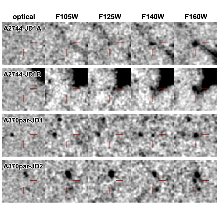
We first discuss the candidate sample based on the HFF dataset in detail, since we have so far only published our search result for the first HFF cluster and its parallel field (A2744; Oesch et al., 2015). As outlined above, we adopt a strict S/N cut for the HFF fields to ensure a reliable candidate selection. Only two of the twelve HFF WFC3/IR fields reveal such candidates in our search. These are the cluster field of Abell 2744 and the parallel field of Abell 370. A few additional, potential sources are shown in the appendix together with a note for each, as to why it was not kept in the final candidate list.
The two candidates behind the cluster Abell 2744 (A2744-JD1A, and A2744-JD1B) were already presented in Oesch et al. (2015). They were originally identified in Zitrin et al. (2014) as two images on either side of the critical curve of one intrinsic, very faint source. While the observed magnitude of these sources is and 26.8 mag, the expected magnification for these images lies in the range 7 to 27 when considering the full range of all HFF lens models. However, most models agree on a magnification factor of for A2744-JD1A. For A2744-JD1B, the distribution of predicted values is bi-modal, clustered around or . Only the higher values result in a self-consistent intrinsic magnitude in the source plane, however, and they are thus more likely. In particular, the magnification factors from the Glafic v3 lens model that are also shown in Table 2.3 reproduce a consistent intrinsic magnitude based on both images of mag. This means that the galaxy is even slightly fainter than the faintest blank-field source found in the HUDF/XDF (XDFj-38126243 Bouwens et al., 2011a; Oesch et al., 2013), which has .
As is evident from Fig 1, the two images lie very close to diffraction spikes of two separate bright foreground sources, which is why photometry for these sources had to be performed manually (see Oesch et al., 2015, for details). Zitrin et al. (2014) further identify a third image of the same source, which is not present in our catalogs, however, as it blended in the halo of a foreground galaxy. Note that our procedure for computing the UV LF is set up in the image plane, and we thus double-count multiple images, which is why we keep both of these candidates separate.
Interestingly, the two candidates in the parallel field of Abell 370 (A370par-JD1, and A370par-JD2), have a similar observed mag and an H-band S/N of 10.1 and 6.4, respectively. They lie about 12 from each other, and are unlikely to be physically associated. While the first candidate is clearly detected in the image, the second source is only seen in , indicating a significantly higher redshift. The second source also lies close to a pair of foreground sources. The magnification factor for these two sources in the parallel field is provided by the lens model of Merten et al. (2011), who find a 1016% residual magnification. The two foreground galaxies in front of A370par-JD2 are not expected to significantly increase this magnification due to galaxy-galaxy lensing given their faintness ( and 28.8, respectively) and inferred low mass.
3.3. Comparison to other HFF Galaxy Searches
Several previous authors have searched for galaxy candidates using the HFF data or parts of it. In particular, McLeod et al. (2016) used the first four HFF cluster and parallel fields in combination with previous CLASH data to identify galaxy candidates based on a photometric redshift selection. In the eight HFF+parallel fields, they present only two candidates in their sample, both with . One of these sources (their ID: HFF1C-10-1) corresponds to our candidate A2744-5887. The other source, HFF4P-10-1, is a robust high-redshift candidate. However, given its color it does not satisfy our selection and it likely lies closer to than . Indeed, it was also selected as a LBG in Ishigaki et al. (2017, ID: HFF4P-3994-7367).
Infante et al. (2015) present one candidate galaxy, ID 8958, in the M0717 cluster field with a photometric redshift of 10.1, which would be the faintest known source given its inferred magnification factor of . This source is also present in our catalogs. However, it only has a S/N of 4.3 in and 3.2 in , and therefore does not pass our final selection. We confirmed this low S/N by hand through aperture photometry using the iraf task qphot. That said, the candidate has an extended morphology along the shear axis of the magnification and appears likely to be a real source. Nevertheless, deeper data would be required to confirm it as a robust candidate, and we do not include it in our analysis. As can be seen later, the extrapolation of our UV LF to the absolute magnitude of this source is consistent with the measurement from Infante et al. (2015) within , however.
The cluster M1149 contains the galaxy MACS1149-JD, first reported in Zheng et al. (2012) based on CLASH data (Postman et al., 2012). The deeper HFF data confirmed the strong Lyman break of the source (Zheng et al., 2017) and a weak continuum detection in an HST grism spectrum is consistent with the photometric redshift of (Hoag et al., 2017). The source lies just barely outside of our color selection, however, with a measured color of , which is why it is not included in our sample.
Finally, Ishigaki et al. (2017) present the results of a high-redshift galaxy search from the full HFF dataset (see also Ishigaki et al., 2015, for an earlier analysis). Interestingly, even though these authors use effectively identical search criteria to what we use, they do not report any galaxy candidates. Since Ishigaki et al. (2017) do not subtract the ICL before running their detection algorithm, however, it is not surprising that they do not recover the candidates in the cluster fields. The reason why they do not identify our candidates in the parallel fields are less obvious, but likely involve differences in the PSF homogenization, source deblending, and aperture photometry (versus isophotal photometry for color and S/N measurements).
3.4. Candidates in Other Search Fields
The searches and galaxy candidates from the remaining fields have already been presented in previous papers (Oesch et al., 2012b, 2014; Bouwens et al., 2016b). They are summarized in Table 3.4. In particular, the sample consists of five reliable sources identified in the XDF and the two GOODS fields. While the XDF source is found close to the detection limit of the data with mag, the four sources identified in the CANDELS/GOODS fields are 3-4 mag brighter with mag. Surprisingly, no candidates were found with intermediate magnitudes, even though the CANDELS-Deep data would have been sensitive down to mag (see the discussion in our previous papers).
Additionally, no candidates were found in the deep HUDF09 parallel fields, or in the three CANDELS Wide fields. The only exception is a lower-quality candidate in the CANDELS/EGS field which was only partially confirmed by a follow-up HST program (Bouwens et al., 2016b). Since it has a 30% chance to be a lower redshift contaminant based on the derived redshift probability distribution function from an SED fit, we have not included it in the current analysis.
| ID | R.A. | Decl. | Ref. | ||
|---|---|---|---|---|---|
| XDFj-38126243 | 03:32:38.12 | -27:46:24.3 | -17.9 | 1,2 | |
| GN-z11aaThis source has been spectroscopically confirmed to lie at by Oesch et al. (2016). It satisfies our color criteria consistent with the expected redshift distribution function of our LBG selection and is thus included in the following analysis. | 12:36:25.46 | 62:14:31.4 | -21.6 | 3,4,5 | |
| GN-z10-2 | 12:37:22.74 | 62:14:22.4 | -20.7 | 3 | |
| GN-z10-3 | 12:36:04.09 | 62:14:29.6 | -20.7 | 3 | |
| GS-z10-1 | 03:32:26.97 | -27:46:28.3 | -20.6 | 3 | |
| Possible Candidate Not Included in Analysis | |||||
| EGS910-2bbThis source only has a probability of 71% to lie at , and is thus not yet included, until deeper follow-up observations confirm its high-redshift nature. | 14:20:44.31 | 52:58:54.4 | -20.8 | 6 | |
3.5. Galaxy Selection Functions
The computation of a UV LF requires an accurate knowledge of the effective selection volume of a given sample. To derive this, we perform extensive completeness and redshift selection simulations, as we have done in previous analyses. In particular, we insert artificial galaxies into the science data and recover these using the same procedure as has been used for the selection of the actual galaxy candidates.
It is clear from our simulations that the detection completeness depends on the light profile and the size distribution of galaxies. This is particularly important in the very high-magnification regions of the HFF cluster datasets (see e.g. Oesch et al., 2015; Bouwens et al., 2017a). Bouwens et al. (2017b) show that both the assumptions on galaxy sizes and the uncertainties of the magnification factors can lead to underestimated selection volumes and hence to overpredicted faint-end slopes of the UV LFs based on the HFF cluster dataset.
To simulate a galaxy population that is as close as possible to reality, we adopt simulations that are based on actual light profiles of LBGs observed in the XDF field that are cloned to higher redshift and scaled to reproduce the observationally constrained size distribution functions at . This technique can only be applied to the blank field datasets, however. In the highest magnification regions of the HFF clusters, the achieved spatial resolution is too high compared to the observed galaxy light profiles even when a size scaling with redshift is taken into account. In the case of the HFF clusters, we thus adopt pure Sersic light profiles for the galaxy population (see also Oesch et al., 2015).
The adopted size distribution functions are based on recent observations of both the redshift and luminosity dependence of galaxy sizes (see e.g. Oesch et al., 2010; Grazian et al., 2012; Huang et al., 2013; Ono et al., 2013; Holwerda et al., 2015; Kawamata et al., 2015; Curtis-Lake et al., 2016; Bouwens et al., 2017a). In particular, we model sizes with lognormal distributions with kpc, and normalizations that depend both on redshift (following ) and on luminosity (according to ). The luminosity dependence is particularly important for the cluster fields where highly magnified galaxies are being found with extremely small sizes (Kawamata et al., 2015; Bouwens et al., 2017a; Vanzella et al., 2017).
| [mag] | [10-4Mpc-3mag-1] |
|---|---|
| **90% upper limit. | |
Finally, the redshift selection function depends on the UV continuum color distribution of galaxies. We therefore assume a distribution of UV continuum slopes that matches the observed values, including its luminosity dependence. We assume no redshift evolution in the distributions beyond (Wilkins et al., 2016), and fix the relation to the one observed at by Bouwens et al. (2014). These are similar to other estimates (see e.g. Finkelstein et al., 2012b; Dunlop et al., 2013).
For each blank field dataset, we insert 100,000 galaxies with the above physical properties and with redshifts ranging from to , and we compute the magnitude dependent completeness, , as well as the redshift selection functions, which depend both on redshift and magnitude . The combination of these two quantities allows us to compute the effective selection volume at a given observed magnitude, , as well as the expected number of observed sources for a given model UV LF (see next section).
As shown, e.g., in Oesch et al. (2015), the completeness also depends on lensing magnification in the HFF cluster fields, with reduced completeness at high magnification factors (since galaxies are not point sources). Following the same procedure of that paper, we thus compute the selection probabilities , which depends on the redshift, the observed magnitude , and the magnification of the simulated galaxies in the cluster fields.
| Assumption | [Mpc-3mag-1] | [mag] | SFRD [/yr]$\dagger$$\dagger$Absolute magnitudes are based on the Glafic lensing models, but include a systematic errorbar that accounts for the model uncertainties. | |
|---|---|---|---|---|
| Fixed M* (at LF)**This is used as our best-fit model throughout the rest of the paper. | (fixed) | |||
| Density Evolution w.r.t | (fixed) | (fixed) | ||
| Fixed M* (at average from ) | (fixed) | |||
| Previous Determinations | ||||
| Bouwens et al. (2015) | (fixed) | (fixed) | $\ddagger$$\ddagger$Computed based on the Schechter function parameters, using a consistent conversion factor and integration limit to allow for a quantitative comparison. | |
| Oesch et al. (2014) | (fixed) | (fixed) | $\ddagger$$\ddagger$Computed based on the Schechter function parameters, using a consistent conversion factor and integration limit to allow for a quantitative comparison. | |
| McLeod et al. (2016) | (fixed) | (fixed) | $\ddagger$$\ddagger$Computed based on the Schechter function parameters, using a consistent conversion factor and integration limit to allow for a quantitative comparison. | |
| Ishigaki et al. (2017) | (fixed) | (fixed) | $\ddagger$$\ddagger$Computed based on the Schechter function parameters, using a consistent conversion factor and integration limit to allow for a quantitative comparison. | |
4. Results
4.1. The UV LF at
In the following sections we first present our observational constraints on the UV LF at based on the combination of all legacy HST fields, and we then compare these to model predictions.
4.1.1 Observational Constraints
Using the candidate sample described in sections 3.2 and 3.4, as well as the completeness and selection functions discussed in section 3.5, we can now estimate the UV LF at . We compute step-wise UV LFs by binning the galaxy population in absolute magnitudes and estimating the effective volume at that magnitude. For each blank field dataset , this can be written as:
| (2) |
Where corresponds to the survey area of field . The total effective volume at a given absolute magnitude is then simply the sum over all survey fields. A similar equation holds for the cluster fields, except that the volume element and the relation between the observed magnitude and the intrinsic absolute magnitude depend on the magnification factor (see, e.g., Oesch et al., 2015).
Uncertainties on the step-wise LF points are derived using Poisson statistics, which dominate the error budget at low number counts even though cosmic variance is significant for the small individual survey fields we probe here. We include the effect of cosmic variance by adding a fractional uncertainty on the expected number counts per field which ranges from 35% in the CANDELS-Wide fields up to 65% in the HFF cluster fields (e.g. Trenti & Stiavelli, 2008; Robertson et al., 2014).
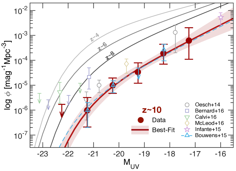
The resulting step-wise UV LF is shown in Fig. 2 and is tabulated in Table 4. As the figure shows, the data points lie significantly below the LF, confirming earlier claims for a significant evolution across . The LF is in excellent agreement with our previous analysis from Bouwens et al. (2015), but the HFF candidates nicely fill in the one upper limit that was still present in earlier LF determinations at . The combined dataset now contains candidates spanning a full 4 mag range.
In order to describe the UV LF, we adopt a Schechter function (Schechter, 1976), whose parameters are fit to the observed number of galaxies in bins of observed magnitudes. Note that the resulting Schechter function is thus not derived from a fit to the stepwise LF, but from an independent fit to the detected number of sources in observed magnitude bins. This is much more accurate as it allows us to properly take into account the redshift distribution as a function of magnitude and the K-correction as a function of redshift. In particular, for a given model UV LF , we compute the expected number of galaxies:
| (3) |
To derive the Schechter function parameters, we then maximize , where is the Poissonian probability, runs over all fields, and runs over the different magnitude bins. Due to the small number of galaxy candidates and the strong degeneracies between the Schechter function parameters, an unconstrained, simultaneous fit of all three parameters is not yet meaningful. We therefore perform different fits with various parameters kept fixed at values motivated by UV LFs. The results are listed in Table 5.
Of particular importance are fits where the characteristic UV luminosity is kept fixed at lower redshift values given the recent finding of very little evolution in this parameter across to . We test two possibilities, one where we fix at the average value found at from both Bouwens et al. (2015) and Finkelstein et al. (2015), i.e. . Using this constraint we find a slightly lower normalization and a somewhat steeper faint end slope than fixing , which is the value of the LF found in Bouwens et al. (2015). However, these two LFs are effectively indistinguishable from each other over the luminosity range we probe here. Indeed, their inferred SFRDs are in excellent agreement, as can also be seen in Table 5. In fact, all three of our LFs give essentially identical SFRDs.
We also list the Schechter function based on a pure density evolution from to relative to the UV LF parameters from Bouwens et al. (2015) (see second row in Table 5), which results in almost exactly an order of magnitude (1.04 dex) lower normalization at than at . Throughout the rest of the paper, we will use the UV LF with , Mpc-3mag-1 and as our best fit model.
4.1.2 Comparison to Previous Measurements
Several early estimates of the UV LF at have been published in the past. However, these have all been based on much smaller search areas than studied here or were based on a subset of the data analyzed in this paper. In Figure 2, we show several of these previous estimates. In particular, these include our own measurements based on the analysis of only the two CANDELS/GOODS+HUDF fields (Oesch et al., 2014). While these earlier measurements are consistent within the uncertainties, the fully combined dataset now indicates an even lower normalization by a factor compared to the lowest of these earlier estimates. In a large part, this is due to the fact that the GOODS-North field appears to contain a significant overdensity of luminous ( mag) galaxies, with three galaxies within a small projected area. Even though the remaining CANDELS-Wide fields would have reached faint enough to find such sources, no reliable candidate could be identified in these datasets, resulting in the lower inferred number density.
Our measured UV LF is in excellent agreement with the previous analysis by Bouwens et al. (2015). This is very encouraging. Our analyses are completely independent, including the simulations of the selection functions and the candidate searches. However, this result is also not surprising given the fact that we use a very similar approach and the fact that the datasets largely overlap, with the exception of the HFF dataset which we newly analyze here. As can be seen, the HFF candidates now provide a measurement of the UV LF at . This magnitude bin previously did not contain any galaxies and corresponded to an upper limit.
Even though the Schechter function parameters of our best-fit model are very different from the ones quoted in Bouwens et al. (2015, see also Table 5), the UV LFs are in very good agreement with each other over the luminosity range we probe, as is shown in Figure 2. Similarly good agreement is found with the Schechter function from Ishigaki et al. (2017).
The only previous UV LF that is clearly discrepant from our new measurement is the one from McLeod et al. (2016). This is based on only one UV LF point, shown in Fig 2, which is higher than our measurement. Based on this one point, McLeod et al. (2016) argued for a much more gradual decline in the cosmic SFRD at . While we discuss the evolution of the cosmic SFRD in detail in section 4.3, it is worth mentioning here that the combination of all the legacy fields is clearly inconsistent with that UV LF (and hence the SFRD) from McLeod et al. (2016). In particular, we can compute how many galaxies we would have expected in our combined dataset assuming their UV LF (based on equation 3). This calculation results in 28 galaxies, i.e., a factor larger than our actual sample of only 9 sources, and can robustly be ruled out. In particular, the McLeod et al. (2016) LF predicts galaxy candidates per HFF cluster field and 4.6 galaxies in the six HFF parallel fields, meaning that in the HFF dataset alone we should have found 16.7 galaxy candidates, four times as many as are present in the data.
Using our best-fit LF, we find much better agreement between the observed and predicted numbers. In particular, this LF predicts a total of 3.3 and 1.3 galaxies to be found in the six HFF clusters and parallel fields combined, respectively – in good agreement with the four candidate images we actually identified.
4.1.3 Comparison to Predicted UV LFs from Models
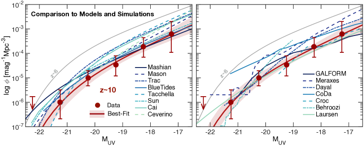
Given the small number of galaxies that we identified in the combined HST dataset, it is interesting to ask whether this might be an indication of a reduced star-formation efficiency in early halos at . To this end, we compare our observational results with several theoretical models and simulations of the UV LF evolution that have been published in the literature over the last few years. These include semi-empirical models tuned to the lower redshift LBG LFs or MFs (e.g., Tacchella et al., 2013; Cai et al., 2014; Mason et al., 2015; Trac et al., 2015; Behroozi & Silk, 2015; Sun & Furlanetto, 2016; Mashian et al., 2016), or semi-analytical models (e.g. Dayal et al., 2014; Cowley et al., 2017), and full hydrodynamical simulations. The latter include UV LFs from the CoDa simulation (Ocvirk et al., 2016), the Croc simulation suite (Gnedin, 2016), BlueTides (Liu et al., 2016; Wilkins et al., 2017), and DRAGONS/Meraxes (Liu et al., 2016), the First Light Project (Ceverino et al., 2017), as well as another simulation by Laursen et al. (2018, in prep).
The comparison to these theoretical predictions is shown in Figure 3. It is evident that the modeled UV LFs decrease in a similar way at compared to what we are finding observationally. Given the vastly different nature of these models, it seems clear that the main driver for this strong evolution is the underlying dark matter halo mass function, which is known to evolve rapidly at these early times (see also discussion in Section 4.4). The differences among the model predictions is typically less than a factor 3-4 over the luminosity range probed by our observations.
Overall the agreement between the observed and simulated UV LFs at is excellent. Several models lie within the uncertainty range of our observed best-fit LF over most of the luminosity range of interest. However, it is important to note that our inferred best-fit Schechter function lies at the low end of all predicted LFs. We further investigate the significance of this by computing the expected number of galaxy candidates that would have been found in the data for each model LF. This is done by folding the model UV LFs through the actual completeness and selection functions of all the different fields (using equation 3) and summing the numbers.
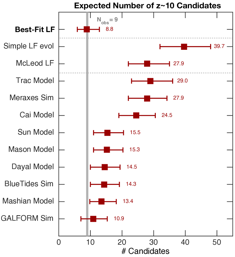
The results of this calculation can be compared to the real number of detected candidates, i.e. 9, which is shown in Figure 4. Interestingly, there seem to be two classes of models. A small number of models predict that about 25-29 galaxies should have been detected. By comparison to the best-fit LF in Fig. 3, it is clear that this discrepancy arises mainly due to a higher normalization of the LF at the faint end (). These models appear to form stars in lower mass galaxies too efficiently and thus overpredict the number of galaxies we should have found in the deepest datasets, i.e., the HUDF/XDF and HFF clusters.
The other set of models predicts galaxy number counts of 13-16, i.e., about 45-70% higher than the observed 9 candidates. Considering the large Poisson+CV uncertainties on these numbers, these models are all within 1-1.5, and the discrepancies are not significant in each individual case. However, the consistently larger predicted numbers suggest a small disconnect with the observations.
The only model that is in close agreement with the observed number counts and also with the observed LF is the one based on GALFORM presented in Cowley et al. (2017). This model predicts about two magnitudes of extinction in the brightest sources, however, which would result in very red predicted UV continuum slopes ( to ). In marked contrast to this, the brightest currently known galaxy candidates show significantly bluer slopes of based on the combination of HST+Spitzer photometry (Wilkins et al., 2016, see also Oesch et al. 2014, Bouwens et al. 2014). It will thus be important to test such models with other measurable quantities.
In summary, the comparison of our observations with theoretical predictions shows that our current candidate galaxy sample lies at the lower end of the predicted range, both for the model UV LFs and in terms of the absolute number of candidates that are present in the data. It will be important to keep this in mind when using these models to define survey strategies for and when predicting higher-redshift number counts.
4.2. Clustering of Galaxies
One possible reason for the low abundance of galaxies in the current sample is obviously cosmic variance. An indication for a very high bias and clustering strength of bright galaxies is provided by the fact that all our nine candidates have been found in only four regions of the sky, while we have searched over 10 general areas. While the CANDELS/GOODS fields have the best data of all the CANDELS fields, the candidates with mag, should have been detectable in any CANDELS field. Yet, only one possible such source was found in the EGS (see Bouwens et al., 2016b). Similarly, only two of the HFF fields contained any candidates, of which one is a multiple imaged source, while the other field (A370-par) contained two sources.
This points to the fact that current surveys may simply be too small or not deep enough to provide an accurate sampling of the galaxy population. It will thus be crucial to obtain deep, wide-area NIR data over the next few years. This will not be possible with JWST, which is not a survey telescope. It will either require a significant investment of HST time or it will have to await new space telescopes such as Euclid or WFIRST.
4.3. The Cosmic SFRD at
The evolution of the cosmic SFRD at has been a matter of debate in the recent literature. In particular, several authors claimed a shallower evolution than has been inferred from the combination of the XDF and GOODS datasets by our team. However, most of these studies were based on the analysis of individual, small fields, and an even smaller number of candidates than studied here. Given the large survey volume in the combined HST dataset, we can now establish the best possible constraint on the SFRD at based on the UV LFs we derived in the previous section.
Thanks to the lensing magnification in the HFF cluster fields, we have further constrained the UV LF to fainter limits than possible with the HUDF/XDF dataset, allowing us to derive the SFRD to lower limits than in our previous analyses without any extrapolation. We use an updated conversion factor from UV luminosity to star-formation rate as discussed in Madau & Dickinson (2014): yrerg s-1 Hz-1. We then integrate the UV LF down to , which corresponds to a SFR limit of yr-1, given this adopted conversion factor .
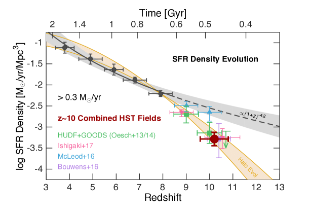
The resulting SFRD values at based on the different assumptions about the UV LF Schechter function parameters are tabulated in Table 5. In particular, our best-fit UV LF results in a SFRD value of M⊙ yr-1 Mpc-3. This is in very good agreement with our previous measurements, where we already pointed out the accelerated evolution at (Oesch et al., 2014; Bouwens et al., 2016b). As can be seen from the table, the SFRD also does not change significantly between our different assumptions about the Schechter function parameters. We consistently find values around M⊙ yr-1 Mpc-3.
It is interesting to compare this measurement to the SFRD at lower redshift. Fig. 5 also shows these measurements based on new dust correction factors motivated by ALMA observations and adding a small contribution from dusty galaxies. In particular, we plot the values assuming an evolving dust temperature from Table 10 in Bouwens et al. (2016a), which were integrated to the same UV luminosity limit. All numbers were adjusted slightly to account for the different conversion factor .
This comparison shows that the SFRD (when integrated to a limit of yr-1) increases by 1.10.2 dex from to . A power law fit to the values results in a SFRD evolution . When extrapolating this to , our measurement lies a factor 5-6 below this trend, similar to our earlier findings, but in contrast to some recent claims by other authors (e.g., McLeod et al., 2016). As noted earlier, the previous measurements of the SFRD that found values consistent with a simple extrapolation of the lower redshift evolution were all based on very small samples or on very limited search volumes. For example, the SFRD measurement by McLeod et al. (2016) was only based on one single point in the UV LF (also shown in Fig 2), and did not include any constraints from the wider area CANDELS data. The combination of all the legacy fields in our analysis significantly increases the search volume and the robustness of the SFRD measurement.
It is also interesting to ask whether a less dramatic evolution of the SFRD is found when integrating to fainter galaxies below our current detection limits. This is indeed the case, given the steeper faint end slope of our best-fit UV LF compared to the reference from Bouwens et al. (2015). However, even when integrating to , i.e. 4 mag below our current detection limit, we still infer a lower SFRD at compared to , albeit with large uncertainties due to the significant extrapolation.
4.4. The SFRD Trend and Dark Matter Halo Buildup
When compared to the SFRD at our measured value lies almost exactly an order of magnitude lower, given that the Schechter function normalization is found to drop by this amount. Such a fast evolution of the SFRD in only 170 Myr from to may sound extreme. However, it is important to note that the halo mass function also evolves extremely fast over this same redshift range. To illustrate this, we compute the cumulative number density of dark matter (DM) halos as a function of redshift using the code HMFcalc555https://github.com/steven-murray/hmf (Murray et al., 2013). Our integration limit of the SFRD (0.3 /yr) roughly corresponds to a dark matter halo mass of at according to several models (e.g., Mason et al., 2015; Mashian et al., 2016; Sun & Furlanetto, 2016). To allow for some variation, we thus compute the cumulative number densities of halos down to and 10.5 as a function of redshift. We then normalize these densities to the measured SFRD at to compare the evolutionary trends, which is also shown in Fig. 5.
The evolution of the cumulative halo mass functions is in excellent agreement with the fast build-up of the SFRD between and , as is evident from the figure. This shows that the observed fast evolution of the SFRD should not have come as a surprise. It is consistent with a model in which the star-formation efficiency is not varying at high redshift (see also Tacchella et al., 2013; Mashian et al., 2016; Stefanon et al., 2017a). Or said another way, a shallower evolutionary trend would require a significant change in the star-formation efficiency within DM halos at high redshift – to zeroth order. Recent results from clustering measurements also provide no compelling evidence of such a change (see Harikane et al., 2017).
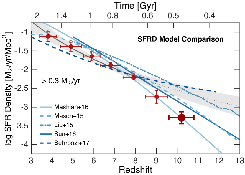
Clearly, our calculation above is simplistic, and more detailed modeling would be valuable, though that is out of the scope of this paper. In Figure 6, we therefore compare the observed SFRD to predictions by some of the same models that were used for the UV LF comparison in section 4.1.3, and for which the SFRDs at have been published. In agreement with the UV LF results, most models predict a significantly higher SFRD at than we observe. Consistent with our findings that the SFRD evolution can be reproduced simply by the DM halo MF build-up, the model by Mashian et al. (2016), which is based on a fixed SFR-Mhalo relation at all redshifts reproduces the observed SFRD trends at . Other models predict higher SFRDs at , and the discrepancy between these predictions are increasing with redshift. As is evident from the Figure, by the predicted SFRD range spans a factor 30 already. This clearly highlights the great power that the JWST will have in testing these model predictions in the near future.
5. Summary
This paper presented a complete and self-consistent analysis of all the prime extragalactic datasets to constrain the evolution of the galaxy UV LF and cosmic star-formation rate densities to . In particular, the imaging data analyzed here span more than 800 arcmin2, and include the HUDF/XDF, the HUDF09/12, the HFF data, as well as all the five CANDELS fields. In particular, we present a small sample of new galaxy candidates in the HFF dataset (see Section 3.2), which are self-consistently folded into the analysis while taking special care of the position- and magnification-dependent completeness in the cluster fields due to lensing.
The main goal of this paper was to exploit all the available Legacy fields in order to derive the best-possible UV LF measurement at before the advent of . While it is clear that the UV LF and the cosmic SFRD continue to decline with increasing redshift, there was some debate in the literature on exactly how fast this decline is between and – accelerated or continuous with respect to ? The HFF dataset provide an excellent, independent test of this, as a power law extrapolation of the UV LF trends to was predicted to reveal more than 25 galaxies in the six HFF clusters+parallel fields. However, after a careful search for galaxies based on the Lyman break, our analysis only revealed four reliable candidate sources/images in these HFF fields, clearly demonstrating that the evolution of the UV LF is faster than at lower redshift, confirming our previous findings of an accelerated evolution.
When combining all the HFF candidates with the five sources previously identified in the HUDF+CANDELS data, we indeed find a best-fit UV LF that is almost exactly a factor lower in normalization compared to (see Fig. 2 and Table 5). This is consistent with several models of galaxy evolution at the level, as we show in Fig. 3. However, the measured UV LFs lie at the low end of all the predictions. In particular, when running the simulated LFs through our selection functions, all models predict a higher number of sources than we find observationally (Fig 4).
Given this measurement of the UV LF, we compute the cosmic SFRD at (integrated over SFRs greater than 0.3 /yr) and confirm our previous measurement of M⊙ yr-1 Mpc-3. This also confirms that the SFRD decreases extremely rapidly at , much faster than the evolution seen at to (hence the term “accelerated evolution”; see Oesch et al., 2012a, 2014). The rapid decline is consistent with the build-up of the DM halo mass function (see Fig 5).
Despite using all legacy fields, only a very small number of reliable galaxies could be identified. This clearly shows that we are reaching the limit of what is possible with to reveal the first generations of galaxies. The discussion about the UV LF at is definitely far from settled - in particular, it is striking that the highest redshift object in our sample (GN-z11) is also the most luminous, which hints at a possible differential evolution of bright vs faint galaxies (see also Oesch et al., 2016).
At , we are now in a situation that is similar to where we were at before the advent of WFC3/IR. Given the immediate revolution within the first few weeks of WFC3/IR data, it can be expected that will provide a similar jump in our knowledge at within the first few weeks of operation. However, it is nevertheless important to realize that the low number density of sources found with and the very rapid evolution of the UV LF seen at will imply that imaging surveys have to be planned carefully in order to be able to push our observational frontier of galaxies to well beyond 400 Myr after the Big Bang.
Appendix A Additional, Plausible HFF Candidates
In Table 6, we list a few additional candidate sources that satisfy our color criteria, but that were nevertheless excluded in our final analysis due to insufficient S/N and other criteria that put their reality into question. For all of these sources, we have performed additional, manual S/N measurements in circular apertures on the ICL subtracted images using the iraf task qphot, which confirmed that the S/N was indeed less than threshold of 6. Several of these sources additionally show extended morphologies (particularly M0416-874), which appear to be affected by correlated background noise on scales of 05, further questioning their reliability.
| ID | R.A. | Decl. | S/N160 | Reason for Exclusion | ||
|---|---|---|---|---|---|---|
| MACS0416 | ||||||
| M0416-874 | 04:16:10.43 | -24:05:02.0 | 5.5 | low S/N | ||
| MACS1149 | ||||||
| M1149-3689 | 11:49:35.54 | 22:24:46.3 | 5.7 | low S/N | ||
| M1149par-2407 | 11:49:44.71 | 22:18:36.7 | 5.1 | low S/N | ||
| M1149par-2491 | 11:49:43.70 | 22:18:40.3 | 5.6 | low S/N | ||
| Abell S1063 | ||||||
| As1063par-2572 | 22:49:20.05 | -44:31:55.8 | 5.2 | low S/N | ||
References
- Ashby et al. (2015) Ashby, M. L. N., Willner, S. P., Fazio, G. G., et al. 2015, ApJS, 218, 33
- Atek et al. (2015) Atek, H., Richard, J., Jauzac, M., et al. 2015, ApJ, 814, 69
- Barone-Nugent et al. (2014) Barone-Nugent, R. L., Trenti, M., Wyithe, J. S. B., et al. 2014, ApJ, 793, 17
- Behroozi & Silk (2015) Behroozi, P. S., & Silk, J. 2015, ApJ, 799, 32
- Bernard et al. (2016) Bernard, S. R., Carrasco, D., Trenti, M., et al. 2016, ApJ, 827, 76
- Bertin & Arnouts (1996) Bertin, E., & Arnouts, S. 1996, A&AS, 117, 393
- Bouwens et al. (2017a) Bouwens, R. J., Illingworth, G. D., Oesch, P. A., et al. 2017a, ApJ, 843, 41
- Bouwens et al. (2017b) Bouwens, R. J., Oesch, P. A., Illingworth, G. D., Ellis, R. S., & Stefanon, M. 2017b, ApJ, 843, 129
- Bouwens et al. (2010) Bouwens, R. J., Illingworth, G. D., González, V., et al. 2010, ApJ, 725, 1587
- Bouwens et al. (2011a) Bouwens, R. J., Illingworth, G. D., Labbe, I., et al. 2011a, Nature, 469, 504
- Bouwens et al. (2011b) Bouwens, R. J., Illingworth, G. D., Oesch, P. A., et al. 2011b, ApJ, 737, 90
- Bouwens et al. (2014) —. 2014, ApJ, 793, 115
- Bouwens et al. (2015) —. 2015, ApJ, 803, 34
- Bouwens et al. (2016a) Bouwens, R. J., Aravena, M., Decarli, R., et al. 2016a, ApJ, 833, 72
- Bouwens et al. (2016b) Bouwens, R. J., Oesch, P. A., Labbé, I., et al. 2016b, ApJ, 830, 67
- Bradley et al. (2014) Bradley, L. D., Zitrin, A., Coe, D., et al. 2014, ApJ, 792, 76
- Cai et al. (2014) Cai, Z.-Y., Lapi, A., Bressan, A., et al. 2014, ApJ, 785, 65
- Calvi et al. (2016) Calvi, V., Trenti, M., Stiavelli, M., et al. 2016, ApJ, 817, 120
- Cardelli et al. (1989) Cardelli, J. A., Clayton, G. C., & Mathis, J. S. 1989, ApJ, 345, 245
- Ceverino et al. (2017) Ceverino, D., Glover, S. C. O., & Klessen, R. S. 2017, MNRAS, 470, 2791
- Coe et al. (2015) Coe, D., Bradley, L., & Zitrin, A. 2015, ApJ, 800, 84
- Coe et al. (2013) Coe, D., Zitrin, A., Carrasco, M., et al. 2013, ApJ, 762, 32
- Cowley et al. (2017) Cowley, W., Baugh, C., Cole, S., Frenk, C., & Lacey, C. 2017, ArXiv e-prints, arXiv:1702.02146
- Curtis-Lake et al. (2016) Curtis-Lake, E., McLure, R. J., Dunlop, J. S., et al. 2016, MNRAS, 457, 440
- Dayal et al. (2014) Dayal, P., Ferrara, A., Dunlop, J. S., & Pacucci, F. 2014, MNRAS, 445, 2545
- Dunlop et al. (2013) Dunlop, J. S., Rogers, A. B., McLure, R. J., et al. 2013, MNRAS, 432, 3520
- Ellis et al. (2013) Ellis, R. S., McLure, R. J., Dunlop, J. S., et al. 2013, ApJ, 763, L7
- Finkelstein (2016) Finkelstein, S. L. 2016, PASA, 33, e037
- Finkelstein et al. (2012a) Finkelstein, S. L., Papovich, C., Ryan, R. E., et al. 2012a, ApJ, 758, 93
- Finkelstein et al. (2012b) Finkelstein, S. L., Papovich, C., Salmon, B., et al. 2012b, ApJ, 756, 164
- Finkelstein et al. (2015) Finkelstein, S. L., Ryan, Jr., R. E., Papovich, C., et al. 2015, ApJ, 810, 71
- Gnedin (2016) Gnedin, N. Y. 2016, ApJ, 825, L17
- Grazian et al. (2012) Grazian, A., Castellano, M., Fontana, A., et al. 2012, A&A, 547, A51
- Grogin et al. (2011) Grogin, N. A., Kocevski, D. D., Faber, S. M., et al. 2011, ApJS, 197, 35
- Harikane et al. (2017) Harikane, Y., Ouchi, M., Ono, Y., et al. 2017, ArXiv e-prints, arXiv:1704.06535
- Hoag et al. (2017) Hoag, A., Bradač, M., Brammer, G. B., et al. 2017, ArXiv e-prints, arXiv:1709.03992
- Holwerda et al. (2015) Holwerda, B. W., Bouwens, R., Oesch, P., et al. 2015, ApJ, 808, 6
- Huang et al. (2013) Huang, K.-H., Ferguson, H. C., Ravindranath, S., & Su, J. 2013, ApJ, 765, 68
- Illingworth et al. (2013) Illingworth, G. D., Magee, D., Oesch, P. A., et al. 2013, ApJS, 209, 6
- Infante et al. (2015) Infante, L., Zheng, W., Laporte, N., et al. 2015, ApJ, 815, 18
- Ishigaki et al. (2017) Ishigaki, M., Kawamata, R., Ouchi, M., Oguri, M., & Shimasaku, K. 2017, ArXiv e-prints, arXiv:1702.04867
- Ishigaki et al. (2015) Ishigaki, M., Kawamata, R., Ouchi, M., et al. 2015, ApJ, 799, 12
- Kawamata et al. (2015) Kawamata, R., Ishigaki, M., Shimasaku, K., Oguri, M., & Ouchi, M. 2015, ApJ, 804, 103
- Kawamata et al. (2016) Kawamata, R., Oguri, M., Ishigaki, M., Shimasaku, K., & Ouchi, M. 2016, ApJ, 819, 114
- Koekemoer et al. (2011) Koekemoer, A. M., Faber, S. M., Ferguson, H. C., et al. 2011, ApJS, 197, 36
- Labbé et al. (2015) Labbé, I., Oesch, P. A., Illingworth, G. D., et al. 2015, ApJS, 221, 23
- Liu et al. (2016) Liu, C., Mutch, S. J., Angel, P. W., et al. 2016, MNRAS, 462, 235
- Livermore et al. (2017) Livermore, R. C., Finkelstein, S. L., & Lotz, J. M. 2017, ApJ, 835, 113
- Lotz et al. (2017) Lotz, J. M., Koekemoer, A., Coe, D., et al. 2017, ApJ, 837, 97
- Madau & Dickinson (2014) Madau, P., & Dickinson, M. 2014, ARA&A, 52, 415
- Mashian et al. (2016) Mashian, N., Oesch, P. A., & Loeb, A. 2016, MNRAS, 455, 2101
- Mason et al. (2015) Mason, C. A., Trenti, M., & Treu, T. 2015, ApJ, 813, 21
- McLeod et al. (2016) McLeod, D. J., McLure, R. J., & Dunlop, J. S. 2016, MNRAS, 459, 3812
- McLure et al. (2013) McLure, R. J., Dunlop, J. S., Bowler, R. A. A., et al. 2013, MNRAS, 432, 2696
- Merlin et al. (2016) Merlin, E., Amorín, R., Castellano, M., et al. 2016, A&A, 590, A30
- Merten et al. (2011) Merten, J., Coe, D., Dupke, R., et al. 2011, MNRAS, 417, 333
- Murray et al. (2013) Murray, S. G., Power, C., & Robotham, A. S. G. 2013, Astronomy and Computing, 3, 23
- Ocvirk et al. (2016) Ocvirk, P., Gillet, N., Shapiro, P. R., et al. 2016, MNRAS, 463, 1462
- Oesch et al. (2015) Oesch, P. A., Bouwens, R. J., Illingworth, G. D., et al. 2015, ApJ, 808, 104
- Oesch et al. (2007) Oesch, P. A., Stiavelli, M., Carollo, C. M., et al. 2007, ApJ, 671, 1212
- Oesch et al. (2010) Oesch, P. A., Bouwens, R. J., Carollo, C. M., et al. 2010, ApJ, 709, L21
- Oesch et al. (2012a) Oesch, P. A., Bouwens, R. J., Illingworth, G. D., et al. 2012a, ApJ, 745, 110
- Oesch et al. (2012b) —. 2012b, ApJ, 759, 135
- Oesch et al. (2013) —. 2013, ApJ, 773, 75
- Oesch et al. (2014) —. 2014, ApJ, 786, 108
- Oesch et al. (2016) Oesch, P. A., Brammer, G., van Dokkum, P. G., et al. 2016, ApJ, 819, 129
- Oguri (2010) Oguri, M. 2010, PASJ, 62, 1017
- Oke & Gunn (1983) Oke, J. B., & Gunn, J. E. 1983, ApJ, 266, 713
- Ono et al. (2013) Ono, Y., Ouchi, M., Curtis-Lake, E., et al. 2013, ApJ, 777, 155
- Planck Collaboration et al. (2016) Planck Collaboration, Ade, P. A. R., Aghanim, N., et al. 2016, A&A, 594, A13
- Postman et al. (2012) Postman, M., Coe, D., Benítez, N., et al. 2012, ApJS, 199, 25
- Robertson et al. (2014) Robertson, B. E., Ellis, R. S., Dunlop, J. S., et al. 2014, ApJ, 796, L27
- Schechter (1976) Schechter, P. 1976, ApJ, 203, 297
- Schenker et al. (2013) Schenker, M. A., Robertson, B. E., Ellis, R. S., et al. 2013, ApJ, 768, 196
- Schlafly & Finkbeiner (2011) Schlafly, E. F., & Finkbeiner, D. P. 2011, ApJ, 737, 103
- Schmidt et al. (2014) Schmidt, K. B., Treu, T., Trenti, M., et al. 2014, ApJ, 786, 57
- Stark (2016) Stark, D. P. 2016, ARA&A, 54, 761
- Stefanon et al. (2017a) Stefanon, M., Bouwens, R. J., Labbé, I., et al. 2017a, ApJ, 843, 36
- Stefanon et al. (2017b) Stefanon, M., Labbé, I., Bouwens, R. J., et al. 2017b, ArXiv e-prints, arXiv:1706.04613
- Sun & Furlanetto (2016) Sun, G., & Furlanetto, S. R. 2016, MNRAS, 460, 417
- Tacchella et al. (2013) Tacchella, S., Trenti, M., & Carollo, C. M. 2013, ApJ, 768, L37
- Trac et al. (2015) Trac, H., Cen, R., & Mansfield, P. 2015, ApJ, 813, 54
- Trenti & Stiavelli (2008) Trenti, M., & Stiavelli, M. 2008, ApJ, 676, 767
- Vanzella et al. (2017) Vanzella, E., Calura, F., Meneghetti, M., et al. 2017, MNRAS, 467, 4304
- Vulcani et al. (2017) Vulcani, B., Trenti, M., Calvi, V., et al. 2017, ApJ, 836, 239
- Wilkins et al. (2016) Wilkins, S. M., Bouwens, R. J., Oesch, P. A., et al. 2016, MNRAS, 455, 659
- Wilkins et al. (2017) Wilkins, S. M., Feng, Y., Di Matteo, T., et al. 2017, MNRAS, 469, 2517
- Windhorst et al. (2011) Windhorst, R. A., Cohen, S. H., Hathi, N. P., et al. 2011, ApJS, 193, 27
- Zheng et al. (2012) Zheng, W., Postman, M., Zitrin, A., et al. 2012, Nature, 489, 406
- Zheng et al. (2017) Zheng, W., Zitrin, A., Infante, L., et al. 2017, ApJ, 836, 210
- Zitrin et al. (2013) Zitrin, A., Meneghetti, M., Umetsu, K., et al. 2013, ApJ, 762, L30
- Zitrin et al. (2014) Zitrin, A., Zheng, W., Broadhurst, T., et al. 2014, ApJ, 793, L12