(Quasi)Periodic revivals in periodically driven interacting quantum systems

Abstract

Recently it has been shown that interparticle interactions generically destroy dynamical localization in periodically driven systems, resulting in diffusive transport and heating. In this work we rigorously construct a family of interacting driven systems which are dynamically localized and effectively decoupled from the external driving potential. We show that these systems exhibit tunable periodic or quasiperiodic revivals of the many-body wavefunction and thus of all physical observables. By numerically examining spinless fermions on a one dimensional lattice we show that the analytically obtained revivals of such systems remain stable for finite systems with open boundary conditions while having a finite lifetime in the presence of static spatial disorder. We find this lifetime to be inversely proportional to the disorder strength.

Introduction.— Dynamical phases of matter, far from thermodynamic equilibrium, have recently attracted significant interest and activity, with periodically driven (Floquet) quantum many-body systems emerging as one of the main research directions. Such systems do not thermalize in the conventional sense due to the continuous injection of energy by the external driving. Nevertheless, they approach a nonequilibrium steady state (NESS) in which the von Neumann entropy is maximized, subject to constraints given by the conservation laws of the system D’Alessio and Rigol (2014); Lazarides et al. (2014a); Ponte et al. (2015). For generic Floquet systems with no conservation laws, the NESS is featureless and cannot be locally differentiated from an infinite temperature state. Some systems can however avoid this fate, due to the existence of an extensive number of conserved quantities analogous to the Generalized Gibbs Ensemble. Noninteracting systems Russomanno et al. (2012); Lazarides et al. (2014b) and interacting systems with sufficiently strong disorder Basko et al. (2006); Lazarides et al. (2015); Abanin et al. (2016) are two examples. The nontrivial NESS of these systems potentially hosts exotic nonequilibrium phenomena such as the recently proposed time-domain crystalline order Khemani et al. (2016); Else et al. (2016, 2017); Ho et al. (2017), which spontaneously breaks the discrete time translation symmetry. Physical observables in discrete time crystals display subharmonic oscillations, namely a periodic time dependence with periods longer than the period of the external drive. Another class of systems which fail to heat up are noninteracting systems exhibiting dynamical localization (DL) — a complete suppression of transport due to the presence of a special drive Dunlap and Kenkre (1986). Generic interactions destroy DL, leading to diffusive transport and eventually a featureless high-entropy steady state Bar Lev et al. (2017). However localization can still be restored by the addition of sufficiently strong static disorder Bairey et al. (2017).

In this work we construct a family of periodic interacting systems exhibiting dynamical localization and for which an initial wave function may show tunable periodic or quasiperiodic revivals. While the revivals are unstable to generic perturbations of our driving protocol, we show that in the presence of disorder of strength $W$ they decay on a time-scale proportional to $1/W$. This offers the possibility of experimental realizations in driven ultracold atoms in optical lattices.

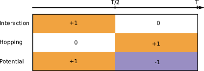
Figure 1: Driving protocol: The driving is alternated between a hopping term operating over the first half period, $t\in\left[0,\frac{T}{2}\right)$, and an interaction term with no hopping operating in the second half period, $t\in\left[\frac{T}{2},T\right)$. There is also an additional external periodic potential which for concreteness was chosen to have an alternating sign over the two half-periods. The figure illustrates the prefactor and the sign of the different terms.

Theory.—We consider a time-dependent $T$-periodic Hamiltonian $\hat{H}(t+T)=\hat{H}(t)$ where the hopping and the interaction do not operate at the same time (see Fig. 1). The Hamiltonian is defined over one period as

$$\hat{H}\left(t\right)=f\left(t\right)\hat{H}_{\text{pot}}+\begin{cases}\sum_{n,m=1}^{L}h_{n-m}\hat{c}_{n}^{\dagger}\hat{c}_{m}&t\in\left[0,\frac{T}{2}\right)\\ \hat{H}_{\text{int}}&t\in\left[\frac{T}{2},T\right)\end{cases}.$$ (1)

Here $L$ is the length of the lattice, $\hat{n}_{m}=\hat{c}_{m}^{\dagger}\hat{c}_{m}$ is the number operator, and $\hat{c}_{m}^{\dagger}$ creates a spinless fermion at site $m$. The function $f\left(t\right)$ is an arbitrary periodic function of time with a period of $T=2\pi/\omega$ and an angular frequency $\omega$. $\hat{H}_{\text{pot}}$ is an external potential with a constant gradient,

$$\hat{H}_{\text{pot}}=\sum_{m=1}^{L}m\hat{n}_{m}.$$ (2)

We will further assume that $\hat{H}_{\text{int}}$ commutes with $\hat{H}_{\text{pot}}$, but is not bilinear in $\hat{c}_{m}^{\dagger}$ and $\hat{c}_{m}$, such that the system is interacting. For notational simplicity we focus here on spinless fermions in one-dimension, though the same formalism with the appropriate modifications applies also for bosons and to higher dimensions. It is convenient to work directly with the propagator of the system,

$$\hat{U}^{\prime}\left(t,t^{\prime}\right)\equiv\mathcal{T}\exp\left[-\mathrm{i}\int_{t^{\prime}}^{t}\mathrm{d\bar{t}}\hat{H}\left(\bar{t}\right)\right],$$ (3)

where $\mathcal{T}$ is the time-ordering operator. Applying the time dependent unitary transformation

$$\hat{V}\left(t\right)=\mathrm{e}^{\mathrm{i}\mathcal{A}\left(t\right)\hat{H}_{\text{pot}}},\quad\mathrm{with}\mathcal{\quad A}\left(t\right)=\int_{0}^{t}\mathrm{d}\bar{t}\,f\left(\bar{t}\right),$$ (4)

to the propagator yields

$$\hat{U}\left(t,t^{\prime}\right)=\hat{V}\left(t\right)\hat{U}^{\prime}\left(t,t^{\prime}\right)\hat{V}^{\dagger}\left(t^{\prime}\right).$$ (5)

and therefore,

$$\mathrm{i}\partial_{t}\hat{U}\left(t,t^{\prime}\right) =\left(\mathrm{i}\partial_{t}\hat{V}\left(t\right)\right)\hat{U}^{\prime}\left(t,t^{\prime}\right)\hat{V}^{\dagger}\left(t^{\prime}\right)$$ (6)

$$+\hat{V}\left(t\right)\left(\mathrm{i}\partial_{t}\hat{U}^{\prime}\left(t,t^{\prime}\right)\right)\hat{V}^{\dagger}\left(t^{\prime}\right).$$

Using Eqs. (3) and (4) we arrive at

$$\mathrm{i}\partial_{t}\hat{U}\left(t,t^{\prime}\right)=\hat{H}^{\prime}\left(t\right)\hat{U}\left(t,t^{\prime}\right),$$ (7)

where

$$\hat{H}^{\prime}\left(t\right) \equiv\hat{V}\left(t\right)\hat{H}\left(t\right)\hat{V}^{\dagger}\left(t^{\prime}\right)-f\left(t\right)\hat{H}_{\text{pot}}.$$ (8)

Since

$$\hat{U}\left(T,0\right)=\mathcal{T}\exp\left[-\mathrm{i}\int_{0}^{T}\mathrm{d\bar{t}}\hat{H}\left({}^{\prime}\bar{t}\right)\right].$$ (9)

Using the assumption $\left[\hat{H}_{\text{int}},\hat{H}_{\text{pot}}\right]=0$, the one-period propagator can be written as $\hat{U}\left(T,0\right)=\hat{U}_{\text{int}}\hat{U}_{\text{nonint}}$, where

$$\hat{U}_{\text{nonint}}\equiv\exp\left[-\mathrm{i}\int_{0}^{T/2}\mathrm{d}\bar{t}\left(\sum_{n,m}\mathrm{e}^{\mathrm{i}\mathcal{A}\left(\bar{t}\right)\left(n-m\right)}h_{n-m}\hat{a}_{n}^{\dagger}\hat{a}_{m}\right)\right]$$ (10)

and

$$\hat{U}_{\text{int}}=\mathrm{e}^{-\mathrm{i}\hat{H}_{\text{int}}T/2}.$$ (11)

Since $\hat{U}_{\text{int}}$ and $\hat{U}_{\text{nonint}}$ do not commute, the system will generally heat up to a featureless stationary state. We note that the noninteracting part of the propagator $\hat{U}_{\text{nonint}}$ corresponds to the propagator of a noninteracting system, exhibiting dynamical localization for appropriately selected ratios of the driving amplitude (of the external potential) to the driving frequency $\omega$. For example, for the hopping matrix,

$$h_{n-m}=\left(\delta_{n,m+1}+\delta_{n,m-1}\right)/2$$ (12)

and drive

$$f\left(t\right)=\begin{cases}-A&-\frac{T}{2}\leq t<0\quad\left(\mod\,T\right)\\ A&0\leq t<\frac{T}{2}\quad\left(\mod\,T\right),\end{cases}$$ (13)

this condition is satisfied for Dunlap and Kenkre (1988)

$$A/\omega=2n\qquad n\in\mathbb{Z\setminus}\{0\}.$$ (14)

In this case $\hat{U}_{\text{nonint}}$ becomes trivial, $\hat{U}_{\text{nonint}}=I$ Dunlap and Kenkre (1986, 1988), and the full propagator reduces to

$$\hat{U}\left(T,0\right)=\mathrm{e}^{-\mathrm{i}\hat{H}_{\text{int}}T/2}$$ (15)

such that the stroboscopic dynamics evolves according to a simple effective Hamiltonian which is identical to $\hat{H}_{\text{int}}$. Since we require $\left[\hat{H}_{\text{int}},\hat{n}_{m}\right]=0$, this propagator is diagonal in the position basis, implying a complete dynamical localization of the model. One can easily show that for interactions with finite support the spreading of any local operator is finite and that for such models even entanglement does not grow with time. The stroboscopic evolution of a many-body wavefunction is generated by the repeated application of the one-period propagator to the wavefunction

$$\left|\psi\left(nT\right)\right\rangle=\hat{U}^{n}\left|\psi\left(0\right)\right\rangle.$$ (16)

This evolution is generally quasiperiodic with multiple incommensurate frequencies leading to correlation functions which generically decay in time. However, periodic stroboscopic revivals of the many-body wavefunction can be obtained if $\hat{U}$ satisfies $\hat{U}^{p}=I$ , such that its spectrum is concentrated on the complex $p-$roots of unity (see Fig. 2). While normally one has no direct access to the properties of $\hat{U}$, for the systems we consider here, its properties are directly determined by the eigenvalues of $\hat{H}_{\text{int}}$ (see Eq. (15)). It is easy to see that for $\hat{H}_{\text{int}}$ with eigenvalues, $E_{\alpha}=J_{z}m_{\alpha}$ and $m_{\alpha}\in\mathbb{Z}$, the propagator in (15) continued to continuous time is periodic with a period of $T^{\prime}=4\pi/J_{z}$, that is, $\hat{U}\left(t+T^{\prime}\right)=\hat{U}\left(t\right)$.

If $T$ and $T^{\prime}$ are commensurate, namely, $T/T^{\prime}=q/p$ with $q,p\in\mathbb{Z}$ the stroboscopic dynamics is periodic with a subharmonic period of $pT$, and the wavefunction exactly revives after $p$ periods of the drive. We will refer to this subharmonic revival mode as $(q:p)$. In case that $T$ and $T^{\prime}$ are incommensurate, the revivals are quasiperiodic, with the wavefunction coming back arbitrary close to its initial state after sufficiently long times. We stress that while in this case the eigenvalues of $\hat{U}$ ergodicaly cover the unit circle (see Fig. 2), since only two incommensurate base frequencies are involved, correlations function will not decay with time.

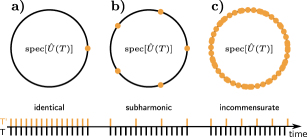
Figure 2: Spectrum of the Floquet operator $\hat{U}(T)$ on the complex unit circle. a) Completely degenerate spectrum, $\hat{U}(T)=1$, with trivial stroboscopic dynamics b) Partially degenerate spectrum which corresponds to complex unit roots (5th root here). The system exhibits subharmonic revival, $\hat{U}(5T)=1$. c) A spectrum which corresponds to a generic quasiperiodic dynamics.

(Quasi)periodic revivals of an arbitrary initial state mean that the state does not obey the discrete time translational symmetry as the Hamiltonian. It is however important to note that this symmetry is not spontaneously broken due to the absence of spatial order in our system Watanabe and Oshikawa (2015).

The results of this section are rigorous, however the proposed driving protocol is fine-tuned. It is therefore pertinent to examine the stability of the revivals, which we do in the next section.

Stability analysis.— To examine the stability of the construction above, we numerically study two simple perturbations: open boundary conditions and a static disordered potential.

We set the hopping matrix $h_{n-m}$ in Eq. (1) as in Eq. (12) , the driving protocol as in (13) and tune to the dynamical localization point (14) with $A=4\pi/T$. The period of the drive is taken to be either $T=3$ or $4$ , such that the corresponding frequencies are much smaller than the single-particle bandwidth. We also use a nearest neighbor interaction of the form

$$\hat{H}_{\text{int}}=J_{z}\sum_{i}\hat{n}_{i}\hat{n}_{i+1}.$$ (17)

As explained in the previous section, this system exhibits (quasi)periodic oscillations of observables for (in)commensurate $T/\left(T^{\prime}\right)=q/p$ with $T^{\prime}=4\pi/J_{z}$. To examine the stability of a subharmonic revival mode $\left(q:p\right)$, we calculate the discrete Fourier transform of the one-particle Green’s function computed at infinite temperature,

$$\tilde{G}_{i}(\omega)=\frac{1}{\sqrt{N}}\sum_{n=0}^{N}\mathrm{e}^{\mathrm{i}\omega Tn}\frac{1}{Z}\text{Tr}\,\left(\hat{c}_{i}^{\dagger}(nT)\hat{c}_{i}\right),$$ (18)

where $N$ is the number of periods we propagate.

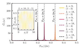
Figure 3: Fourier transform of the one particle Green’s function, $\tilde{G}_{i}\left(\omega\right)={\cal FT}\left[G_{i}(t)\right]$, in a clean open chain of lengths $L=18$ and $L=9$ for different interaction strengths tuned to different subharmonic modes $(1:p)$, using a driving period of $T=4$. The inset shows the stroboscopic dynamics in the real time domain for $p=5$, which is not periodic in $T$, but periodic in $5T$

Instead of calculating the trace over the full Hilbert space, which would require the full diagonalization of the Hamiltonian, we approximate it by an expectation value calculated with respect to a random state, $\left|\psi_{0}\right\rangle$, sampled randomly from the Haar measure Popescu et al. (2006). This approximation is of exponential precision in the dimension of the Hilbert space Levy (1939). To further reduce the error we average our results over 10-100 such random initial states. The calculation of the one-particle Green’s function is then reduced to the propagation of two vectors $\left|\psi_{L}\left(n\right)\right\rangle=\hat{U}^{n}\left|\psi_{0}\right\rangle$ and $\left|\psi_{R}\left(n\right)\right\rangle=\hat{U}^{n}\hat{c}_{i}\left|\psi_{0}\right\rangle$, according to the driving protocol (13) illustrated in Fig. 1, and taking the expectation value $G_{i}\left(n\right)=\left\langle\psi_{L}\left(n\right)|\hat{c}_{i}^{\dagger}|\psi_{R}\left(n\right)\right\rangle$. We note that this requires to consider two sectors of the Hamiltonian, effectively doubling the dimension of the Hilbert space. The repeated application of $\hat{U}\left|\psi_{0}\right\rangle$ can be efficiently computed utilizing the sparse structure of the problem Al-Mohy and Higham (2011) (for additional details on the method see Sec. VA in Ref. Luitz and Lev (2016)). This allows us to study systems of sizes up to $L=21$ for very late times $t\geq 1000$.

Since the theoretical treatment of the previous section applies to either periodic boundary conditions or infinite system sizes, it is important to verify that the effect is robust for open boundary conditions. In Fig. 3, we show $\tilde{G}_{i}(\omega)$ for a system with open boundary conditions and an interaction strength tuned to several subharmonic revival modes, $\left(1:p\right)$. We observe a perfect revival of the Green’s function, leading to a sharp peak in the Fourier transform exactly at $\omega T=1/p$, without a significant dependence on the size of the system up to the accessible number of driving periods. We have checked that this result prevails for various driving frequencies $\omega$ smaller than the single particle bandwidth.

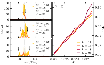
Figure 4: Stability of the subharmonic revival mode $(1:3)$ to the introduction of static disorder. Left: Fourier transform of the Green’s function, $\tilde{G}_{i}\left(\omega\right)$ for different disorder strengths, $W$, for the subharmonic revival mode $(1:3)$. Here, $T=3$ and $L=18$ ($L=21)$ using $1000$ ($300$) driving periods respectively. Black arrows indicate the estimate of the width of the revival mode for the $L=18$ data (see text) Right: The width of the spectral peak on the left as a function of the disorder strength. The visible small fluctuations originate both from statistical and systematic sampling errors.

Any experimental realization of our system will be subject to imperfections. To model such imperfections we introduce a static disorder potential $\hat{H}_{\text{dis}}=\sum_{i}v_{i}\hat{n}_{i}$ with $\hat{v}_{i}$ uniformly distributed in the interval $\left[-W,W\right]$. In the presence of disorder, the subharmonic revival modes acquire a life-time, $\tau\left(W\right)$ which we estimate by measuring the broadening of the corresponding spectral peaks. The width of the spectral peak is taken as the maximal distance of satellite peaks (indicated by black arrows in Fig. 4) which have a spectral intensity of at least 10% of the one of the central spectral peak. We observe a linear dependence of the spectral width on the disorder strength, which appears converged with the size of the system. The life-time of the subharmonic revival modes therefore scales as $\tau\left(W\right)\sim 1/W$.

Discussion.—We have constructed a family of interacting periodically driven systems exhibiting dynamical localization, which can be tuned to have subharmonic periodic or quasiperiodic revivals of the many-body wavefunction. Namely, all physical observables show (quasi)periodic dependence, over time-scales longer than the period of the drive. The revivals are independent of the initial state of the system and originate from the special structure of the eigenvalues of the one-period propagator (see Fig. 2).

Despite not satisfying the conditions for spontaneous symmetry breaking outlined in Ref. Watanabe and Oshikawa (2015), our construction serves as a unique example of a nontrivial interacting quantum system with tunable revivals. Our stability analysis shows that while the revivals are stable under a change of boundary conditions, introduction of static disorder leads to a finite lifetime inversely proportional to the disorder strength. It is therefore possible that with proper control of the disorder, subharmonic revivals could also be seen in cold atoms experiments.