Learning Wireless Networks’ Topologies Using Asymmetric Granger Causality

Abstract

Sharing spectrum with a communicating incumbent user (IU) network requires avoiding interference to IU receivers. But since receivers are passive when in the receive mode and cannot be detected, the network topology can be used to predict the potential receivers of a currently active transmitter. For this purpose, this paper proposes a method to detect the directed links between IUs of time multiplexing communication networks from their transmission start and end times. It models the response mechanism of commonly used communication protocols using Granger causality: the probability of an IU starting a transmission after another IU’s transmission ends increases if the former is a receiver of the latter. This paper proposes a non-parametric test statistic for detecting such behavior. To help differentiate between a response and the opportunistic access of available spectrum, the same test statistic is used to estimate the response time of each link. The causal structure of the response is studied through a discrete time Markov chain that abstracts the IUs’ medium access protocol and focuses on the response time and response probability of 2 IUs. Through NS-3 simulations, it is shown that the proposed algorithm outperforms existing methods in accurately learning the topologies of infrastructure-based networks and that it can infer the directed data flow in ad hoc networks with finer time resolution than an existing method.

I Introduction

Consider the scenario where a cognitive network is sharing spectrum with one or more incumbent networks. Spectrum sharing by opportunistic spectrum access requires that the cognitive network avoid interference to the receivers in the incumbent networks. At present, there is extensive work on the detection of transmitters in the field of spectrum sensing [1] but significantly less on identifying receivers. In particular, existing methods for coexistence in TV white space [2] and the Spectrum Access System (SAS) of the Citizen’s Broadband Radio Service (CBRS) [3] detect transmissions and enforce a protection region around the transmitters where CRs are not allowed to transmit. The size of this protection region is designed such that the CRs outside the protection region do not cause harmful interference to any incumbent receivers located on the border of the incumbent transmitter’s service area. On the other hand, if we can identify the potential receivers, we can enforce a smaller protection region around the receivers rather than the transmitters.

Identifying the current receivers in a network of communicating IUs is difficult because receivers are inherently passive when they are in receiving mode and because it is costly for the cognitive network to decode the packets in the incumbent network. Instead, we can use the IUs’ network topology to identify the potential receivers of currently active transmitters. This observation motivates us to learn the IUs’ network topology, i.e., the directed links between IUs. Similar to existing work, we will focus on learning the network topology of time multiplexing incumbent networks.

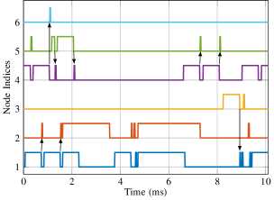
Figure 1: Example activity traces of 802.11n networks from NS-3 simulation for a 6 IU system consisting of two infrastructure based networks with APs indexed 1 and 4. Arrows indicate some transmit-response pairs.

I-A Existing Work

In literature, the temporal patterns in IU transmissions have been used to learn network topology. The features used include transmission start and end times, frame durations, and inter-arrival times. We shall base our work on a similar input. As has been shown in [4], we do not need prior knowledge of the IUs’ communication protocols to distinguish IUs and detect the transmission activities of each IU. Hence, we do not require knowledge of the IUs’ communication protocol to obtain these inputs. Note that the location of the IUs is not useful in learning their network topology because the networks need not be geographically separated.

One set of existing methods to learn network topology are based on the causal nature of time multiplexing communication protocols: A transmission by an IU is likely to cause a response, say in the form of an acknowledgement, by its intended receiver after a fixed but unknown delay. Examples of such networks include the 802.11 family of protocols, Bluetooth, and TDD-LTE. Fig. 1 shows an example of the transmit-response pairs in activity sequences of 802.11n networks simulated in NS-3. Using this observation, [5, 6] model the responses as a causal structure in the IUs’ transmission activity time series. They propose methods to identify pairs of communicating IUs by detecting IUs that have a higher probability of transmitting after another. This paper is also based on the same idea.

Another approach to this problem recognizes that the directed links in an ad hoc network correspond to the end-to-end routes and learns those routes directly [7]. The authors propose an algorithm that clusters IUs that have similar distributions of packet lengths and inter-arrival times to infer that these IUs participate in the same data flow. Since they do not infer the ordering of the IUs in the route, we need additional information, e.g., locations, to identify potential receivers of each IU along the route. Their method also requires the network to have the same data rates on all links. In addition, in infrastructure-based networks, receiving IUs typically do not repeat the transmission and are unlikely to have the same packet lengths as the transmitting IU.

I-B Challenges and Contributions

The primary challenge with using causality to detect responses is that if two IUs are not communicating with each other but are located close enough to interfere with each other, then their collision avoidance mechanisms will ensure that their transmission activities are not independent. This implies that, unlike typical Granger causality literature, the causality between two IUs is non-zero even if they are not communicating with each other.

The second challenge is the time varying nature of network topology: the inferences of our algorithm are only useful if they are valid for some period of time. We will show that the proposed algorithm learns network topology in the order of 100ms. Since network topology does not change that frequently, cognitive radios can use the learned topology for making inferences for some period of time in the future.

Thirdly, it can be argued that inferences on the entire network should be made simultaneously through a multivariate method (such as graphical LASSO) since there will be multiple causal relationships in the incumbent network. Instead, we will use a common feature of communication protocols to argue that testing each pair of IUs independently is sufficient for learning the network topology rather than making an inference for the entire network simultaneously. Note that [5] also tests pairs of IUs independently.

To help ensure that we detect responses, we choose to detect the causality from the transmission end times of transmitter IU to the transmission start times of the receiver IU. Hence, we propose a binary hypothesis test for each ordered pair of IUs based on the asymmetric form of Granger causality as compared to the symmetric form used in [5, 6]. For this test, we propose a non-parametric test statistic that does not assume a linear model between the transmission start and end times of the pair of IUs being tested.

Since such a test may confuse frequent opportunistic spectrum access as responses, we study the response time in existing time multiplexing communication protocols to note that the response time is shorter than the idle time and is required to be roughly constant. Based on these observations and verification from NS-3 simulations, we propose an algorithm to estimate the response time from the same test statistic mentioned above. We call the combination of the test statistic and this estimation algorithm as the Asymmetric Transfer Entropy to Learn Network Topology (ATELNeT) algorithm.

To study the effects of dependent transmission activities, we propose a Markov chain model that abstracts the IUs’ medium access protocol and focuses on the response time and retransmission times of a pair of IUs. From this model, we verify that the response time will be estimated correctly and show that both false alarm as well as detection probability increase as the frames become shorter and more frequent.

The rest of this paper is organized as follows. Section II describes our system model and assumptions. Section III defines Granger causality, relates different tests from literature to existing work on topology learning, and proposes a non-parametric test statistic for asymmetric Granger causality. Section IV motivates and proposes our ATELNeT algorithm. The Markov chain model for 2 IUs is discussed in Section V. NS-3 simulations of infrastructure-based and ad hoc networks are presented in Section VI. The paper is concluded in Section VII.

II System Model

We consider a scenario with $M$ IUs indexed as $1,\ldots,M$. We assume that these IUs have been identified by a system such as that proposed in [4], by decoding physical layer headers, localization, or fingerprinting their radios. In addition, we assume that this system provides a time sequence of the activity of each IU, sampled periodically at $T_{s}$ intervals, such that the activity of the $m$’th IU is denoted by $a_{m}[t]=1$ if it is transmitting at time $tT_{s}$ and 0 otherwise. For the purpose of this work, we shall assume that these sequences are error-free and that each sequence is of length $N$ samples.

We denote the pair-wise links between these IUs by a binary matrix $L\in\{0,1\}^{M\times M}$ such that $L_{i,j}=1$ if there is a link from IU $i$ to IU $j$.

For a time series $X[t]$ and positive integer $\tau$, we use $X^{(\tau)}[t]$ to denote $X[t-1],\ldots,X[t-\tau]$. We use $\mathds{1}_{\{\,\cdot\,\}}$ to denote an indicator variable. For developing our algorithm, we will denote the sampled time series of transmission start time indicators of the $i$’th IU by $S_{i}[t]\triangleq\mathds{1}_{\left\{a_{i}[t]=1,a_{i}[t-1]=0\right\}}$. We denote the sampled indicator time series of the end of transmissions of the $i$’th IU by $E_{i}[t]\triangleq\mathds{1}_{\left\{a_{i}[t+1]=0,a_{i}[t]=1\right\}}$.

II-A Assumptions about IUs’ Medium Access Protocol

We define a transmit-receive link by the receiver’s act of responding to a signal by the transmitter. Consider a link from IU $i$ to IU $j$. Assuming a half duplex communication link, the receiver $j$ has to wait for the transmitter $i$ to finish transmitting before $j$ can respond. Thus, the end of a transmission by IU $i$ causes the start of a transmission by IU $j$ after a short time interval. We call this time interval as the response time or causal lag and denote it by $\tau_{i,j}$. It consists of both processing times as well as hardware delays such as the Rx-to-Tx turnaround time. For example, this is defined in the IEEE 802.11 standard [8, §10.3.7] as the Short Inter-Frame Space (SIFS) which is computed as

$$\text{aSIFSTime}= \text{ aRxPHYDelay}+\text{aMACProcessingDelay}$$

$$+\text{aRxTxTurnaroundTime}.$$

Similarly, LTE-TDD has a fixed length guard period between downlink and uplink pilots as part of a special subframe [9, §4.2]. Bluetooth [10] has a fixed interframe space T_IFS between every Master to Slave and Slave to Master transmission. Finally, each of these standards define a maximum allowed variation in the response time. It is to be expected that such a response time will feature in future time division multiplexing communication protocols. Hence, we incorporate the response time in our system model and say that there is link $i\rightarrow j$ if $E_{i}[t]=1$ causes $S_{j}[t+\tau_{i,j}]=1$ where $\tau_{i,j}$ is the response time of that link. Note that we do not mean to assume that $j$ transmits a response to every transmission by $i$, but if $j$ does respond to $i$’s transmission, then it will do so $\tau_{i,j}$ time after $i$’s transmission ends. We also assume that the variation in response times on a link is significantly smaller than $T_{s}$.

Our second assumption is that the time interval between two successive transmissions by an IU is longer than the response time for any link originating from that IU. Mathematically,

$$P(a_{i}[n+t]=1|a_{i}[n-1]=1,a_{i}[n]=0)=0$$

if $t<\max_{j\in\{1,\ldots,M\}}\{\tau_{i,j}:L_{i,j}=1\}$. This assumption is based on the fact that communication protocols are designed to avoid interference to the response. For example, the 802.11 standard specifically sets the NAV field to include the acknowledgement frame’s duration [8].

Finally, we assume that we know an upper bound $\tau_{\max}$ on $\tau_{i,j}$ for all $i,j\in\{1,\ldots,M\}$ such that $i\rightarrow j$.

III Granger Causality

Similar to existing work, we are going to base our work on the idea of Granger causality. In this section, we briefly introduce the concept, theoretical models, and tests used in existing literature. We relate these methods to the existing works on learning network topology and then propose a new test statistic for testing asymmetric Granger causality.

The concept of Granger causality was first proposed for macroeconomic analysis [11]. As defined in [11], a time series $X[t]$ is said to Granger cause a time series $Y[t]$ if the minimum mean square error (MMSE) estimator of $Y[t]$ given $X^{(\infty)}[t]$ and $Y^{(\infty)}[t]$ has lower error than the MMSE estimator of $Y[t]$ given only $Y^{(\infty)}[t]$. Since the MMSE estimator of $Y[t]$ given $X^{(\infty)}[t]$ and $Y^{(\infty)}[t]$ is $\operatorname{\mathbb{E}}[Y[t]|X^{(\infty)}[t],Y^{(\infty)}[t]]$ [12], we can say that $X$ Granger causes $Y$ if $Y[t]$ is not conditionally independent of $X^{(\infty)}[t]$ given $Y^{(\infty)}[t]$. The causal lag defined in [11] corresponds to the sampled response time $\tau_{\cdot,\cdot}$ in our system model. Since the causal lag is unknown, it is usually estimated from the input data by either the Akaike Information Criterion (AIC) or Bayesian Information Criterion (BIC) [13]. Thus, the problem of testing Granger causality between a pair of time series $X$ and $Y$ is a binary hypothesis problem where the null hypothesis ($\mathcal{H}_{0}$) is that $X$ does not Granger cause $Y$.

III-A Models and Tests

Most methods in literature for testing Granger causality are based on regression but are modified with domain knowledge specific to the problem under consideration [13]. Specifically, a causal link from $X[t]$ to $Y[t]$ is modeled as a vector autoregressive model such as [11, 13]

$$Y[t]=\sum_{\tau=1}^{\tau_{\max}}\alpha_{1,\tau}X[t-\tau]+\sum_{\tau=1}^{\tau_{\max}}\beta_{1,\tau}Y[t-\tau]+\xi_{1}[t]$$ (1)

where $\alpha_{1,\tau}$ and $\beta_{1,\tau}$ are the parameters of the regression and $\xi_{1}[t]$ is the residual noise. Similarly, the null hypothesis is modeled as

$$Y[t]=\sum_{\tau=1}^{\tau_{\max}}\beta_{0,\tau}Y[t-\tau]+\xi_{0}[t]$$ (2)

with $\beta_{0,\tau}$ being the regression parameters and $\xi_{0}[t]$ the residual noise. Therefore, the null hypothesis is modeled by the coefficients $\alpha_{1,\tau}$ in this model being zero.

In [5], the authors use this linear model for testing causality between every pair of IUs on disjoint observation windows. Their hard fusion algorithm then fuses the topologies learned in each window using the majority rule. For individual windows, the hard fusion algorithm proposed in [5] uses the test statistic

$$g_{i\rightarrow j} \triangleq\left(\frac{\sum_{t=1}^{N-\tau}|\hat{\xi}_{0}[t]|^{2}-\sum_{t=1}^{N-\tau}|\hat{\xi}_{1}[t]|^{2}}{\sum_{t=1}^{N-\tau}|\hat{\xi}_{1}[t]|^{2}}\right)\frac{N-3\tau-1}{\tau}$$ (3)

$$\sim F(\tau,N-3\tau-1)$$ (4)

where $\hat{\xi}_{1}[t]$ and $\hat{\xi}_{0}[t]$ are the estimates of $\xi_{1}[t]$ and $\xi_{0}[t]$ respectively and the authors assume that both $\xi_{0}[t]$ and $\xi_{1}[t]$ have zero-mean Gaussian distributions and equal variances. The threshold is chosen using (4) to satisfy a given false alarm probability. In their soft fusion algorithm, the authors compute the average causality magnitude [14] of a link

$$F_{i\rightarrow j}=\ln\left(\frac{\operatorname{\mathbb{E}}\left[|\xi_{1}[t]|^{2}\right]}{\operatorname{\mathbb{E}}\left[|\xi_{0}[t]|^{2}\right]}\right).$$ (5)

for each window. The network topology is inferred as those links with average causality magnitude greater than the average of all pairs of IUs.

Transmission start times have been considered as continuous time point processes and modeled as multivariate Hawkes processes in [6]. In the Hawkes process model, an event in one time series increases the probability of an event occurring on other time series for a short period of time. The support of these impact functions were recently shown to be equivalent to Granger causality [15]. There is a rich body of literature learning Hawkes point processes and might be useful for learning Granger causality in multivariate systems as done in [16]. With respect to our system model, we are using sampled activity sequences as input and not point processes.

Finally, an information theoretic non-parametric test for Granger causality has been proposed in [17]. The author of [17] proposed the conditional mutual information of $Y[t]$ and $X^{(\tau)}[t]$ given $Y^{(\tau)}[t]$:

$$T_{X\rightarrow Y}\triangleq\sum \Bigg{[}P\left(Y[t],X^{(\tau)}[t],Y^{(\tau)}[t]\right)$$

$$\quad\left.\times\log\frac{P\left(Y[t]|X^{(\tau)}[t],Y^{(\tau)}[t]\right)}{P\left(Y[t]|Y^{(\tau)}[t]\right)}\right]$$ (6)

as a test statistic called transfer entropy for testing whether $X[t]$ Granger causes $Y[t]$. In (6), the summation is over all possible values of $X^{(\tau)}[t]$,$Y^{(\tau)}[t]$, and $Y[t]$. The author proposes a binary hypothesis test with $T_{X\rightarrow Y}=0$ as the null hypothesis for no causality and $T_{X\rightarrow Y}>0$ as the alternate hypothesis denoting a causal relationship. We shall base our proposed method on a similar test statistic described below.

III-B Asymmetric Granger Causality

In this work, we are going to use an asymmetric form of Granger causality loosely based on that proposed in [18]. Consider three time series $X[t]$, $Y_{1}[t]$, and $Y_{2}[t]$. We will say that $X[t]$ asymmetrically Granger causes $Y_{2}[t]$ given $Y_{1}[t]$ if $Y_{2}[t]$ and $X^{(\infty)}[t]$ are not conditionally independent given $Y_{1}^{(\infty)}[t]$. Note the absence of $Y^{(\infty)}_{2}[t]$ in this definition. Thus, we can think of $X[t]$ and $Y_{1}[t]$ as events representing potential causes while $Y_{2}[t]$ denotes the events representing effects.

Here, $Y_{1}[t]$ and $Y_{2}[t]$ typically describe different events on an underlying common sequence while $X[t]$ describes events on a second time sequence. For example, in our proposed algorithm, $Y_{1}[t]$ and $Y_{2}[t]$ will correspond to the end and start transmission events respectively of one IU while $X[t]$ will denote the end transmission events of another IU.

Similar to Granger causality, we use a finite history $\tau$ while testing asymmetric Granger causality. We propose an asymmetric transfer entropy as our test statistic

$$A_{X\rightarrow Y_{2}|Y_{1}}(\tau)\triangleq\sum \Bigg{[}P\left(Y_{2}[t],X^{(\tau)}[t],Y_{1}^{(\tau)}[t]\right)$$

$$\quad\left.\times\log\frac{P\left(Y_{2}[t]|X^{(\tau)}[t],Y_{1}^{(\tau)}[t]\right)}{P\left(Y_{2}[t]|Y_{1}^{(\tau)}[t]\right)}\right]$$ (7)

where the summation is over all values taken by $X^{(\tau)}[t]$, $Y_{1}^{(\tau)}[t]$, and $Y_{2}[t]$. The test statistic shall compare between the same hypotheses as described above for [17]. The motivation and use of this test statistic for learning network topology is described in the next section.

IV Proposed Method: Asymmetric Transfer Entropy to Learn Network Topology (ATELNeT)

In this section, we will be proposing a test for detecting causal links between ordered pairs of IUs at a time. In general, it is true that there may be a performance benefit in detecting all links simultaneously through a multivariate test. However, as mentioned earlier in Section II-A, communicating protocols are usually designed to avoid interfering with the response of the receiver. Hence, by focusing on the response time of each link, we expect that other IUs’ transmissions will not interfere with the testing of a given link. Hence, we also propose a method for estimating the response time from the test statistic. We will also be proposing an additional linear regression based test similar to that of [5] for comparing the performance gain from the choice of nonlinear model against the linear model.

IV-A Proposed Test Statistic for Transmit-Receive Pair

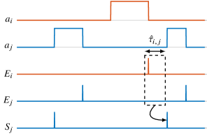
Figure 2: Example inputs to our proposed algorithm for testing link $i\rightarrow j$. The algorithm tests the causality from the input values in the dashed rectangle to the transmission start indicator. The response time $\tau_{i,j}$ needs to be estimated.

As mentioned above, we propose testing every ordered pair $i$, $j$ of IUs independently. Similar to [17], we consider two hypotheses: the null hypothesis $\mathcal{H}_{0}(i,j)$ represents $i\not\rightarrow j$ and the alternate hypothesis $\mathcal{H}_{1}(i,j)$ represents $i\rightarrow j$. To specifically detect the responses transmitted by IU $j$ to transmissions of IU $i$, we test whether $E_{i}[t]$ asymmetrically Granger causes $S_{j}[t]$ given $E_{j}[t]$. Fig. 2 shows the inputs that we use for testing this asymmetric causality. Since there is no reason to assume a linear model for $E_{i}[t]$, $E_{j}[t]$, and $S_{j}[t]$, we use the non-parametric asymmetric transfer entropy (7) that we proposed in Section III-B:

$$\hat{A}_{E_{i}\rightarrow S_{j}|E_{j}}(N,\hat{\tau}_{i,j})\mathop{\gtrless}_{\mathcal{H}_{0}(i,j)}^{\mathcal{H}_{1}(i,j)}\lambda(\hat{\tau}_{i,j})$$ (8)

where $\hat{A}_{E_{i}\rightarrow S_{j}|E_{j}}(N,\hat{\tau}_{i,j})$ is the empirical estimate of $A_{E_{i}\rightarrow S_{j}|E_{j}}(\hat{\tau}_{i,j})$ computed from $N$ activity samples with a response time of $\hat{\tau}_{i,j}$, $\lambda(\hat{\tau}_{i,j})$ is a threshold that depends on the response time. The response time $\hat{\tau}_{i,j}$ will need to be estimated from the data and the threshold $\lambda(\,\cdot\,)$ will be computed from the distribution of $\hat{A}_{E_{i}\rightarrow S_{j}|E_{j}}$ as described next.

We derive the asymptotic distribution of $\hat{A}_{E_{i}\rightarrow S_{j}|E_{j}}$ in Appendix A. Our derivation is similar to that of the asymptotic distribution of $\hat{T}_{X\rightarrow Y}$ in [19]. We show that for large $N$ and a given causal lag $\tau$, $2(N-\tau)\hat{A}_{E_{i}\rightarrow S_{j}|E_{j}}(N,\tau)$ has distribution $\chi^{2}_{d_{i,j}}$ under the null hypothesis $\mathcal{H}_{0}(i,j)$ and distribution $\chi^{2}_{d_{i,j}}\left(2(N-\tau)A_{E_{i}\rightarrow S_{j}|E_{j}}(\tau)\right)$ under the alternate hypothesis $\mathcal{H}_{1}(i,j)$ where $\chi^{2}_{d}$ is a central $\chi^{2}$ distribution with $d$ degrees of freedom and $\chi^{2}_{d}(c)$ is a non-central $\chi^{2}$ distribution with $d$ degrees of freedom and non-centrality parameter $c$.

We choose the threshold $\lambda(\tau)$ such that the probability of false alarm is asymptotically bounded above by a parameter $P_{\text{FA}}$:

$$\lambda(\tau)\triangleq\chi^{-2}_{d_{i,j}}(1-P_{\text{FA}})$$ (9)

where $\chi^{-2}_{d}(\,\cdot\,)$ is the inverse cumulative distribution function of a central $\chi^{2}$ random variable with $d$ degrees of freedom.

Note that we have assumed that $A_{E_{i}\rightarrow S_{j}|E_{j}}(\tau)=0$ under the null hypothesis. Though this is a common hypothesis in the Granger causality literature as well as [5, 6], we will show below that $A_{E_{i}\rightarrow S_{j}|E_{j}}(\tau)>0$ even if $\mathcal{H}_{0}(i,j)$. Since this value is unknown a priori, we choose $A_{E_{i}\rightarrow S_{j}|E_{j}}(\tau)=0$ to define the null hypothesis. Fortunately, both the model analyzed in Section V and simulations in Section VI show that $A_{E_{i}\rightarrow S_{j}|E_{j}}(\tau)$ is sufficiently small that we can still use this typical null hypothesis of $A_{E_{i}\rightarrow S_{j}|E_{j}}(\tau)=0$.

Next, we need to estimate the degrees of freedom $d_{i,j}$. As per the derivation in Appendix A, $d_{i,j}$ is the difference in the number of parameters for models under the alternate hypothesis $\mathcal{H}_{1}(i,j)$ and the null hypothesis $\mathcal{H}_{0}(i,j)$. Since $E_{i}[t],E_{j}[t],S_{j}[t]\in\{0,1\}$, the number of parameters in either model is simply the number of independent values in the appropriate joint probability mass function. Next, our assumption that the retransmission time is longer than the response time means that if $E_{j}[t-\tau]=1$ for some $1\leq\tau\leq\hat{\tau}_{i,j}$ then $S_{j}[t]=0$. It also means that $\sum_{\tau=1}^{\hat{\tau}_{i,j}}E_{j}[t-\tau]\leq 1$ and $\sum_{\tau=1}^{\hat{\tau}_{i,j}}E_{i}[t-\tau]\leq 1$. Hence, the number of parameters under null hypothesis is $\hat{\tau}_{i,j}+1$ and under the alternate hypothesis is $(\hat{\tau}_{i,j}+1)^{2}$. Hence, the degrees of freedom are

$$d_{i,j}=\hat{\tau}_{i,j}(\hat{\tau}_{i,j}+1).$$ (10)

IV-B Proposed Algorithm to Estimate Response Time of a Link

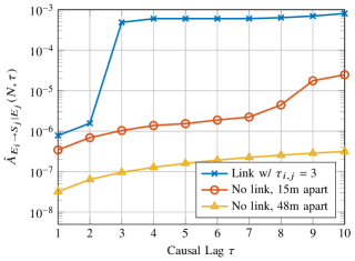
Figure 3: Asymmetric transfer entropy of pairs of IUs in NS-3 simulated 802.11n networks computed with increasing causal lags. Parameters: $T_{s}\ 5\mu$s and observation duration 10s.

Estimating the response time $\hat{\tau}_{i,j}$ depends on its invariance. In particular, if the variance in response time is significantly smaller than the sampling time of the link, then the response is likely to be received at either $\tau_{i,j}$ or $\tau_{i,j}+1$ with high probability. Hence, $A_{E_{i}\rightarrow S_{j}|E_{j}}(\tau_{i,j})$ will be significantly higher than $A_{E_{i}\rightarrow S_{j}|E_{j}}(\tau_{i,j}-1)$. This intuition will be revisited analytically in Section V. From NS-3 data of 3 pairs of 802.11n IUs, Fig. 3 shows that $\hat{A}_{E_{i}\rightarrow S_{j}|E_{j}}(N,\tau)$ increases sharply at $\tau=3$, i.e., after SIFS of $16\mu$s, if there is a link but not if the pair do not have a link. For the pair of IUs that do not have a link but are close to each other, Fig. 3 also shows a slight increase in $\hat{A}_{E_{i}\rightarrow S_{j}|E_{j}}(N,\tau)$ at the lags after the minimum retransmission time, i.e., after DIFS of 34$\mu$s.

Based on this discussion, we estimate $\hat{\tau}_{i,j}$ such that

$$\hat{A}_{E_{i}\rightarrow S_{j}|E_{j}}(N,\hat{\tau}_{i,j})>\alpha\hat{A}_{E_{i}\rightarrow S_{j}|E_{j}}(N,\hat{\tau}_{i,j}-1)$$ (11)

for a parameter $\alpha>1$. Pseudocode for estimating $\hat{\tau}_{i,j}$ is provided in Algorithm 1. Starting from the maximum response time $\tau_{\max}$, we keep reducing the estimated response time $\hat{\tau}_{i,j}$ until the asymmetric transfer entropy reduces by the factor $\alpha$. For the alternate hypothesis, this finds the correct response time as will be seen from the simulations. On the other hand, the test statistic does not change rapidly under the null hypothesis and the algorithm stops at $\tau=1$. As we will discuss in Section V, under the null hypothesis, the asymmetric transfer entropy is minimum at $\tau=1$. Hence, this estimate of the response time ensures the best match with the null hypothesis assumption that $A_{E_{i}\rightarrow S_{j}|E_{j}}(\tau_{i,j})=0$.

Algorithm 1 Estimating response time for link $i\rightarrow j$

1:$\tau_{\max}\in\mathbb{N}$, $\alpha\in\mathbb{R}_{+}$, $\hat{P}\left(E_{i}^{(\tau_{\max})}[t],E_{j}^{(\tau_{\max})}[t],S_{j}[t]\right)$

2:$\tau\leftarrow\tau_{\max}$

3:$r\leftarrow\hat{A}_{E_{i}\rightarrow S_{j}|E_{j}}(N,\tau-1)/\hat{A}_{E_{i}\rightarrow S_{j}|E_{j}}(N,\tau)$

4:while $\tau>1$ and $r>\alpha$ do

5:     $\tau\leftarrow\tau-1$

6:     $r\leftarrow\hat{A}_{E_{i}\rightarrow S_{j}|E_{j}}(N,\tau-1)/\hat{A}_{E_{i}\rightarrow S_{j}|E_{j}}(N,\tau)$

7:end while

8:$\hat{\tau}_{i,j}\leftarrow\tau$

9:$\hat{\tau}_{i,j}$

IV-C Linear Test for Asymmetric Causality

The ATELNeT algorithm proposed above is different from the existing work in two aspects: the choice of testing the asymmetric rather than symmetric Granger causality and the transfer entropy test statistic as opposed to the regression based approaches. In order to understand the performance gain of the two aspects separately, we propose a second test statistic based on linear regression.

Similar to the approach of [5] and with notation analogous to that of (1)-(2), we model the null hypothesis $\mathcal{H}_{0}(i,j)$ as

$$S_{j}[t]=\sum_{\tau=1}^{\tau_{i,j}}\beta_{0,\tau}E_{j}[t-\tau]+\xi_{0}[t].$$ (12)

and the alternate hypothesis $\mathcal{H}_{1}(i,j)$ as

$$S_{j}[t]=\sum_{\tau=1}^{\tau_{i,j}}\alpha_{1,\tau}E_{i}[t-\tau]+\sum_{\tau=1}^{\tau_{i,j}}\beta_{1,\tau}E_{j}[t-\tau]+\xi_{1}[t].$$ (13)

We use the test statistic of (3) and threshold based on (4) as per the false alarm constraint $P_{\text{FA}}$: $F^{-1}_{\tau_{i,j},N-3\tau_{i,j}-1}(1-P_{\text{FA}})$ where $F^{-1}_{a,b}$ is the inverse cumulative $F$ distribution with parameters $a$ and $b$. Unlike [5], we do not split the input into windows.

Note that this approach requires separate estimation of the response time $\tau_{i,j}$.

V Analysis of Asymmetric Transfer Entropy in Shared Channel

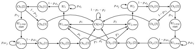
Figure 4: Markov chain model for two users sharing a wireless channel under the assumption of no collisions.

In this section, we propose a Markov chain model of 2 IUs $i$ and $j$ for studying the behavior of $A_{E_{i}\rightarrow S_{j}|E_{j}}$ as we vary the causal lag $\tau$, the frame lengths, inter-arrival times, and the probability of one IU responding to another. Ideally, this requires modeling the MAC protocol of the incumbent network. But to avoid restricting our study to a single MAC protocol and for analytical tractability, we re-use the observation in Section II-A that IUs will not interfere with each others’ responses to construct a simplified discrete time Markov chain model of only 2 IUs. The Markov chain’s state transitions occur every $T_{s}$ seconds. We make the following assumptions:

1. No collisions between IUs $i$ and $j$

2. Response time $\tau_{ij}=3=\tau_{ji}$ for each link

3. Transmissions and responses are at least 2 samples long

4. Packet sources have stationary distributions for arrival times and packet lengths

5. (Frame length - 1) for IU $i$ is a geometric random variable with parameter $1-p_{di}$

6. No retransmissions within $\tau_{ij}$ or $\tau_{ji}$.

7. A response does not cause the source to send a response.

Note that assumption 5 is justified in the system model described in Section II.

We will describe the model from the point of view of IU $i$ transmitting a new frame and IU $j$ responding (or not). The model is symmetric in $i$ and $j$. The states of the model are chosen such that in each state, the indicator variables $E_{i}[t]$, $E_{j}[t]$, $S_{i}[t]$, and $S_{j}[t]$ take exactly one value each.

The model begins in the central state $\text{Ch}[\infty]$ that represents the unoccupied channel with no active transmissions or responses. From this state, either IU may start transmitting a new frame with probability $p_{i}$ or $p_{j}$ respectively. These parameters are related to the frame duration $T_{i,\text{frame}}$ and idle time $T_{i,\text{idle}}$ (in seconds) of the IUs as follows.

$$p_{i}=\frac{T_{s}}{\operatorname{\mathbb{E}}[T_{i,\text{frame}}]+\operatorname{\mathbb{E}}[T_{i,\text{idle}}]}\text{, }p_{j}=\frac{T_{s}}{\operatorname{\mathbb{E}}[T_{j,\text{frame}}]+\operatorname{\mathbb{E}}[T_{j,\text{idle}}]}$$ (14)

Without loss of generality, assume IU $i$ starts transmitting. The continued transmission of IU $i$ is modeled by the state $\text{IU}_{i}$ which has a self loop of probability $p_{d_{i}}$ to model the frame length as 1 + $G$ where $G$ is a geometric random variable. The parameter $p_{d_{i}}$ is related to the expected frame duration (in seconds) by

$$p_{d_{i}}=1-\frac{T_{s}}{\operatorname{\mathbb{E}}[T_{i,\text{frame}}]-T_{s}}.$$ (15)

When the frame ends, the channel is modeled to be vacant for two time samples in states $\text{Ch}_{i}[1]$ and $\text{Ch}_{i}[2]$. Since we have assumed that the response time is 3 samples for both links, the model can transition from state $\text{Ch}_{i}[2]$ to a response state $\text{IU}_{j,\text{resp}}~{}\text{start}$ with a response probability $p_{r_{j}}$ or continue to a state of unoccupied channel $\text{Ch}_{i}[3]$ with probability $1-p_{r_{j}}$. If the latter transition occurs, then the system will simply transition back to the initial unoccupied channel state $\text{Ch}[\infty]$.

Instead, if IU $j$ begins transmitting a response, then we model the response length $T_{j,\text{response}}$ by the state $\text{IU}_{j,\text{resp}}$ that has a self loop of probability $p_{dr_{j}}$:

$$p_{dr_{j}}=1-\frac{T_{s}}{\operatorname{\mathbb{E}}[T_{j,\text{response}}]-T_{s}}.$$ (16)

When the response ends, the channel is modeled as being unoccupied for at least two more time instants because of our fifth and sixth assumption above. From state $\text{Ch}_{ij}[3]$, either IU may start transmitting with the original probabilities $p_{i}$ and $p_{j}$. If neither begins transmitting, then the channel is unoccupied and the system returns to the state $\text{Ch}[\infty]$.

The model for IU $j$ transmitting is identical.

It should be noted that the model in Fig. 4 defines a scenario where two users sharing the same channel always detect each other’s transmissions and never collide. Hence, the causality in this model is slightly higher than a more practical scenario.

For the purposes of the following discussion, we consider the null hypothesis to be $\mathcal{H}_{0}(i,j)$ as defined earlier. Since the model is symmetric in $i$ and $j$, without loss of generality, we consider only the alternate hypothesis of $\mathcal{H}_{1}(i,j)$. Unless mentioned otherwise, we set $p_{r_{i}}=0$, i.e., $i$ never responds to $j$’s transmissions.

V-A Computing Asymmetric Transfer Entropy from the Model

TABLE I: Values of $E_{i}^{(3)}[t]$, $E_{j}^{(3)}[t]$, $S_{i}[t]$, and $S_{j}[t]$ for each state and notation for steady state probability

State	$E_{i}^{(3)}[t]$			$E_{j}^{(3)}[t]$			$S_{i}[t]$	$S_{j}[t]$	Notation
$\text{Ch}[\infty]$	0	0	0	0	0	0	0	0	$p^{*}_{ch[\infty]}$
IU${}_{i,\text{start}}$	0	0	0	0	0	0	1	0	$p^{*}_{is}$
IUi	0	0	0	0	0	0	0	0	$p^{*}_{i}$
Ch${}_{i}[1]$	1	0	0	0	0	0	0	0	$p^{*}_{ch_{i}[1]}$
Ch${}_{i}[2]$	0	1	0	0	0	0	0	0	$p^{*}_{ch_{i}[2]}$
Ch${}_{i}[3]$	0	0	1	0	0	0	0	0	$p^{*}_{ch_{i}[3]}$
IU${}_{j,\text{resp}}$ start	0	0	1	0	0	0	0	1	$p^{*}_{jr_{s}}$
IU${}_{j,\text{resp}}$	0	0	0	0	0	0	0	0	$p^{*}_{jr}$
Ch${}_{ij}[1]$	0	0	0	1	0	0	0	0	$p^{*}_{ch_{ij}[1]}$
Ch${}_{ij}[2]$	0	0	0	0	1	0	0	0	$p^{*}_{ch_{ij}[2]}$
Ch${}_{ij}[3]$	0	0	0	0	0	1	0	0	$p^{*}_{ch_{ij}[3]}$
IU${}_{j,\text{start}}$	0	0	0	0	0	0	0	1	$p^{*}_{js}$
IUj	0	0	0	0	0	0	0	0	$p^{*}_{j}$
Ch${}_{j}[1]$	0	0	0	1	0	0	0	0	$p^{*}_{ch_{j}[1]}$
Ch${}_{j}[2]$	0	0	0	0	1	0	0	0	$p^{*}_{ch_{j}[2]}$
Ch${}_{j}[3]$	0	0	0	0	0	1	0	0	$p^{*}_{ch_{j}[3]}$
IU${}_{i,\text{resp}}$ start	0	0	0	0	0	1	1	0	$p^{*}_{jr_{s}}$
IU${}_{i,\text{resp}}$	0	0	0	0	0	0	0	0	$p^{*}_{jr}$
Ch${}_{ji}[1]$	1	0	0	0	0	0	0	0	$p^{*}_{ch_{ji}[1]}$
Ch${}_{ji}[2]$	0	1	0	0	0	0	0	0	$p^{*}_{ch_{ji}[2]}$
Ch${}_{ji}[3]$	0	0	1	0	0	0	0	0	$p^{*}_{ch_{ji}[3]}$

TABLE II: Probability mass function for $E_{i}^{(3)}[t]$, $E_{j}^{(3)}[t]$, $S_{i}[t]$, and $S_{j}[t]$.

$E_{i}^{(3)}[t]$			$E_{j}^{(3)}[t]$			$S_{i}[t]$	$S_{j}[t]$	Probability
0	0	0	0	0	0	0	0	$p^{*}_{ch[\infty]}+p^{*}_{i}+p^{*}_{jr}+p^{*}_{ir}+p^{*}_{j}$
0	0	0	0	0	0	0	1	$p^{*}_{js}$
0	0	0	0	0	0	1	0	$p^{*}_{is}$
0	0	0	0	0	1	0	0	$p^{*}_{ch_{j}[3]}+p^{*}_{ch_{ij}[3]}$
0	0	0	0	0	1	1	0	$p^{*}_{ir_{s}}$
0	0	0	0	1	0	0	0	$p^{*}_{ch_{j}[2]}+p^{*}_{ch_{ij}[2]}$
0	0	0	1	0	0	0	0	$p^{*}_{ch_{j}[1]}+p^{*}_{ch_{ij}[1]}$
0	0	1	0	0	0	0	0	$p^{*}_{ch_{i}[3]}+p^{*}_{ch_{ji}[3]}$
0	0	1	0	0	0	0	1	$p^{*}_{jr_{s}}$
0	1	0	0	0	0	0	0	$p^{*}_{ch_{i}[2]}+p^{*}_{ch_{ji}[2]}$
1	0	0	0	0	0	0	0	$p^{*}_{ch_{i}[1]}+p^{*}_{ch_{ji}[1]}$

To compute $A_{E_{i}\rightarrow S_{j}|E_{j}}(\tau_{i,j})$ in this model, we first need to compute the joint probability mass function of $E_{i}^{(\tau_{i,j})}[t]$, $E_{j}^{(\tau_{i,j})}[t]$, and $S_{j}[t]$. As mentioned above, the states of the model were designed such that each state had exactly one value for these three time series. This correspondence is listed in Table I. Here, $E_{i}^{(3)}[t]$ is listed in the order $E_{i}[t-1],E_{i}[t-2],E_{i}[t-3]$. Similarly for $E_{j}^{(3)}[t]$. Using this correspondence, we can write the joint probability mass function of $E_{i}^{(\tau_{i,j})}[t]$, $E_{j}^{(\tau_{i,j})}[t]$, and $S_{j}[t]$ in terms of the steady state probabilities of this Markov chain model. The joint probability mass function is listed in Table II.

The steady state probabilities have been derived in Appendix B by solving the appropriate simultaneous equations. The asymmetric transfer entropy for various lags can then be expressed in terms of our model’s parameters by using Table II to compute individual terms in the summation of (7). These expressions for causal lags up to 3 are derived in Appendix C. Unfortunately, the algebraic expressions themselves do not provide much insight into the behavior of the test statistic due to the large number of terms involved. Therefore, we study the behavior of the test statistic numerically by varying its various parameters, viz., the probability of starting a new transmission $p_{i}$ and $p_{j}$, the frame lengths through $p_{d_{i}}$ and $p_{d_{j}}$, the probability of IUs responding to each other $p_{r_{i}}$ and $p_{r_{j}}$, and the length of the response frames through $p_{dr_{i}}$ and $p_{dr_{j}}$.

V-B Effect of increasing causal lag

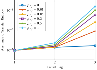
Figure 5: Asymmetric transfer entropy for $i\rightarrow j$ computed from our model for various response probabilities and causal lags. System: Expected $T_{\text{on}}+T_{\text{off}}=10$ms, frame duration 3.33ms, response duration 333$\mu$s, $T_{s}=5\mu$s.

We begin by studying the increase of asymmetric transfer entropy for the link $i\rightarrow j$ with increasing causal lag. As Fig. 5 shows, $A_{E_{i}\rightarrow S_{j}|E_{j}}(\tau)$ increases with $\tau$ for all response probabilities $p_{r_{j}}$, but the rate of increase also increases with $p_{r_{j}}$. Most importantly, $A_{E_{i}\rightarrow S_{j}|E_{j}}(\tau)$ increases significantly at $\tau=3$. This matches our intuition in Section IV-B where we expected this sudden increase due to the fact that a response is likely to occur with high probability at lag 3. We can also use Fig. 5 to choose the parameter $\alpha$ in Algorithm 1. Fig. 5 shows that $A_{E_{i}\rightarrow S_{j}|E_{j}}(3)$ is at least 10 times larger than $A_{E_{i}\rightarrow S_{j}|E_{j}}(2)$ for even $p_{r_{j}}=0.01$. Hence, we suggest $\alpha=10$ is an appropriate choice for the parameter.

V-C Effect of frame durations and idle time

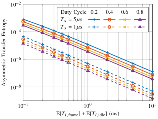
Figure 6: Theoretical asymmetric transfer entropy under the null hypothesis as the expected duration between the start of consecutive transmissions is varied

One reason for studying this model is to understand how $A_{E_{i}\rightarrow S_{j}|E_{j}}(1)$ behaves under the null hypothesis. For this purpose, we set $p_{r_{j}}=0=p_{r_{i}}$. As discussed above, the estimated response time for a null hypothesis link will be 1. From Appendix C, we can express $A_{E_{i}\rightarrow S_{j}|E_{j}}(1)$ as

$$A_{E_{i}\rightarrow S_{j}|E_{j}}(1)= \frac{\rho_{0}-2p_{j}-p_{i}}{\rho_{0}}\log\left(1-\frac{p_{i}}{\rho_{0}-2p_{j}}\right)$$

$$+\frac{\rho_{0}-p_{j}}{\rho_{0}}\log\left(\frac{\rho_{0}-p_{j}}{\rho_{0}-p_{j}-p_{i}}\right)$$ (17)

where $\rho_{0}=1+4p_{i}+p_{i}(1-p_{d_{i}})^{-1}+4p_{j}+p_{j}(1-p_{d_{j}})^{-1}$. Now, for the purposes of this study, let us set $p_{i}=p_{j}$ and rewrite $p_{d_{i}}$ and $p_{d_{j}}$ using (15) in the form of a duty cycle percentage. Then, Fig. 6 shows that $A_{E_{i}\rightarrow S_{j}|E_{j}}(1)$ increases as the frames become shorter and more frequent. It also shows that reducing the sampling interval $T_{s}$ reduces $A_{E_{i}\rightarrow S_{j}|E_{j}}(1)$. Intuitively, this makes sense because a shorter $T_{s}$ implies more samples in the interval between transmissions. We shall revisit (17) and Fig. 6 in Section VI for understanding the effect of increasing $N$.

V-D Effect of increasing response probability

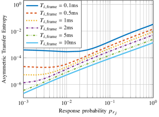
Figure 7: Asymmetric transfer entropy under alternate hypothesis for increasing response probability. Both IUs $i$ and $j$ have equal probability of starting a new transmission and frame length distributions. Parameter: Response duration 250$\mu$s, mean idle time = 100$\mu$s.

As is to be expected, the asymmetric transfer entropy increases with the probability $p_{r_{j}}$ of IU $j$ responding to IU $i$. Fig. 7 shows that this is true only for a sufficiently large response probability depending on the frame length when a constant idle time is maintained. Together with the discussion for Fig. 6, we infer that for short and frequent transmissions, the asymmetric transfer entropy under the null hypothesis is equivalent to that for a small response probability. Hence, Fig. 7 further highlights the difficulty of detecting causality for IUs with short frequent transmissions.

VI Simulation Results

In this section, we study the performance of learning the topology of 802.11n networks through NS-3 simulations. Note that 802.11n uses time division multiplexing opportunistic spectrum access through its Distributed Coordination Function (DCF). The simulation uses a 20MHz wide channel in the 5GHz band with a datarate of 19.5Mbps. The response time (called SIFS) for this setting is 16$\mu$s while the minimum interval (called DIFS) between the end of one transmission and the start of another is 34$\mu$s. We use this set up for studying infrastructure-based networks of 2 access points (APs) located 40m apart and stations (STAs) uniformly distributed in a disc of radius 15m. NS-3’s OnOffApplications are set up for both uplink and downlink flows at all STAs and APs. These applications have exponentially distributed on and off times. The parameters used for the NS-3 simulations of each of the following simulations are listed in Table III.

For our Monte Carlo simulations, we present results for different infrastructure-based topologies after averaging over time. That is, each topology is simulated for up to 1000 seconds and each of the topology learning algorithms are run on non-overlapping time windows of the obtained activity sequences. The length of these windows is described for each of the scenarios below. The learning algorithms were implemented in MATLAB for ease of development. We measure the performance of the algorithms as the average fraction of links detected and the average number of extra links, i.e., pairs of IUs erroneously detected as being linked. We consider links without direction.

In this section, we will use the Monte Carlo simulations to compare our proposed ATELNeT algorithm with the hard and soft fusion algorithms proposed in [5], the Hawkes process based method proposed in [6], and the linear asymmetric test proposed in Section IV-C. Then, we will present a comparison to the algorithm proposed in [7] for learning end-to-end routes in ad hoc networks. Finally, we will compare the computational complexity of the different algorithms.

VI-A Comparison of Parameters

TABLE III: Simulation parameters for the simulations in Section VI

Parameters	ROC	Duration	Network Size
Protocol	802.11n	802.11n	802.11n
Number of APs	2	2	2
Number of STAs per AP	3	3	1 to 6
Uplink mean on time	1ms	1ms	1ms
Uplink mean off time	10ms	10ms	10ms
Downlink mean on time	None	None	1ms
Downlink mean off time	None	None	10ms
Observation duration	60ms, 600ms	1ms to 5s	1s

Though the input for each of the algorithms mentioned above are the same binary activity sequences $a_{m}[n]$, each of these methods uses a different sampling interval and causal lag. For the hard and soft fusion algorithms of [5], we input the activity sequences sampled at $T_{s}=20\mu$s, used a window size of 60ms, and set the causal lag to 8 samples, i.e., 160$\mu$s as per the authors recommendations. Since [6] studies the continuous time point process of the transmission start times, we input the absolute start times of each transmission. A causal lag of 160$\mu$s was used via an exponentially decaying kernel.

For ATELNeT, we ensure $T_{s}\tau_{\max}$ is greater than the minimum idle time for any IU. In general, we want $T_{s}$ to be shorter than the minimum response time for any pair of IUs and, as Fig. 6 indicates, $T_{s}$ should be as small as possible. For the 802.11 family, the minimum idle time varies from 34$\mu$s to 50$\mu$s. Hence, we choose $T_{s}=5\mu$s and $\tau_{\max}=10$, i.e., maximum causal lag of 50$\mu$s.

For the linear test for asymmetric Granger causality, we choose the same sampling interval $T_{s}=5\mu$s, but set the causal lag as 3 samples to match the response time of the 802.11n system being simulated.

VI-B Comparison of Test Statistics

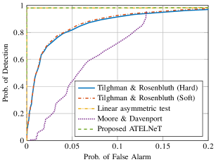
(a) Observed duration: 60ms

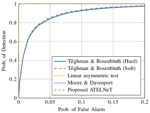
(b) Observed duration: 600ms

Figure 8: ROC of the topology learning algorithm for a system of 2 APs 40m apart and 3 STAs each. For null hypothesis, test statistics for two STAs associated with different APs were used. For alternate hypothesis, test statistics for an AP and an associated STA were used. Test statistics were computed for 1000 non-overlapping windows of duration 60ms in (a) and 600ms in (b).

We begin by studying the receiver operating characteristics (ROC) for the test statistics proposed in [5, 6] and Section IV. For the hard fusion algorithm proposed in [5], we used $g_{i\rightarrow j}$ from (3) as the test statistic. For the soft fusion algorithm also proposed in [5], we used the causality magnitude $F_{i\rightarrow j}$ from (5). For the algorithm proposed in [6], we used their influence matrix as the test statistic.

First, we used 60ms long observation periods to plot the ROC in Fig. LABEL:sub@fig:topology_roc_best_60ms. We note that both test statistics proposed in [5] have almost identical curves. On the other hand, the algorithm proposed in [6] appears to have an upper limit on the achievable detection probability. Furthermore, since the authors do not propose a minimum strength required for detecting the causal connection, their threshold is chosen to be zero, i.e., they operate at the upper limit of the detection probability as seen in Fig. LABEL:sub@fig:topology_roc_best_60ms. Hence, their proposed method suffers from a large false alarm rate as will be seen in the later results as well. Finally, test statistics of both ATELNeT, i.e., $\hat{A}_{E_{i}\rightarrow S_{j}|E_{j}}(N,\hat{\tau}_{i,j})$, and linear asymmetric test, i.e., (3), have approximately the same ROC.

Next, Fig. LABEL:sub@fig:topology_roc_best_600ms shows the ROC for observation periods of 600ms. Since both algorithms proposed in [5] use windows of length 60ms, the ROC for their test statistics do not change with increasing observation periods. However, the algorithm proposed in [6] does improve its ROC making it a viable candidate for testing the binary hypotheses. The linear asymmetric test as well as ATELNeT have almost identical and perfect ROC curves.

The perfect nature of the ROC curves in Fig. LABEL:sub@fig:topology_roc_best_600ms indicates that any of the three methods – that proposed in [6] and those we propose in Section IV – should be able to achieve almost perfect detection of the network topology by an appropriate choice of thresholds. However, the simulation results below will show that the thresholds chosen for each algorithm are suboptimal. We believe this is due to two facts: the threshold is chosen to have constant false alarm and the null hypothesis in all these works models zero causality.

VI-C Performance vs. Observation Duration

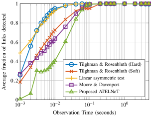
(a) Average fraction of undirected links detected

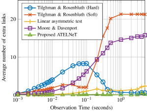
(b) Average number of extra links detected

Figure 9: Performance of inferring network topology as observation duration increases. System: 2 802.11n APs with 3 STAs each.

Increasing the observation period or, equivalently, the number of samples $N$ has multiple effects. First, the non-stationary nature of the communication protocols means that more responses are observed on each link. Secondly, with increasing number of samples, each of the methods is able to detect weaker causal relationships. Hence, the false alarm rate of each of the methods, including ATELNeT, increases with increasing observation period or number of samples.

Fig. 9 shows the performance of each of these algorithm in learning the topology of the system with 2 APs and 3 STAs associated with each AP. As expected, the fraction of links detected correctly increases with the observation period. The higher detection rate of the linear tests is also associated with a higher number of extra links as seen in Fig. LABEL:sub@fig:topology_sim_duration_extra. Both algorithms proposed in [5] attempt to reduce the number of extra links by splitting the observed period into windows of equal duration and fusing the topologies inferred on each window. As seen in Fig. LABEL:sub@fig:topology_sim_duration_extra, the hard fusion algorithm of [5] is more effective at reducing the number of extra links detected than the soft fusion algorithm. Note that the maximum number of extra links detected by the hard fusion algorithm is at about 60ms, i.e., the duration of a single window.

The proposed ATELNeT algorithm detects the least number of extra links. Since the linear asymmetric test also detects significantly fewer extra links than the methods of [5], we believe this performance gain is due to testing asymmetric Granger causality instead of symmetric Granger causality. Note that the linear asymmetric test does not use windowing or fusion.

We can also see this rise from our model using (17). By the non-central $\chi^{2}$ distribution of $\hat{A}_{E_{i}\rightarrow S_{j}|E_{j}}(N,1)$, we can write the false alarm probability $P_{\text{FA}}$ as

$$P_{\text{FA}}=Q_{1}\left(\sqrt{2(N-1)A_{E_{i}\rightarrow S_{j}|E_{j}}(1)},\sqrt{\lambda(1)}\right)$$ (18)

where $Q_{1}(\cdot,\cdot)$ is Marcum’s Q function. Hence, $P_{\text{FA}}$ increases with $N$ due to the monotonic nature of the Marcum’s Q function. Now, our Markov chain model has more dependencies than the actual system due to assumptions such as lack of collisions. Therefore, (18) provides an upper bound for $P_{\text{FA}}$ rather than an equality. For example, the system considered in Fig. 9 has $A_{E_{i}\rightarrow S_{j}|E_{j}}(1)$ of the order of $10^{-7}$ under the null hypothesis as per Fig. 6. For a 5s observation period, i.e., $N=10^{6}$, (18) tells us that the false alarm probability is bounded above by 0.0653 while the simulation resulted in a false alarm probability of 0.0083.

VI-D Performance as Network Size Increases

(a) Average fraction of undirected links detected

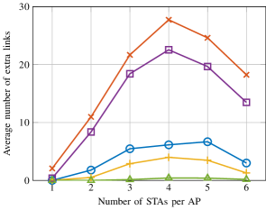
(b) Average number of extra links detected

Figure 10: Performance of inferring network topology as the number of STAs increases. System: 2 802.11n APs with up to 6 STAs each.

(a) At 35s

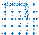
(b) At 40s

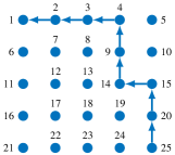
(c) At 41s

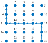
(d) At 43s

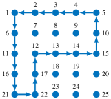
(e) At 111s

(f) Output of [7] over full 150s

Figure 11: Links learned from activity sequences of 25 IU ad hoc network. Data flow was set up from IU 25 to IU 1 from time 30s to 80s and from IU 21 to IU 5 from time 110s to 140s. 1s long observation periods were used for learning network topology and activity sequences were sampled at $T_{s}=5\mu$s. Each link has 1Mbps data rate and 9$\mu$s response time.

In Fig. 10, we compare the performance of learning the network topology as the number of STAs associated with each AP increase. The trends are similar to that seen in Fig. 9. The linear asymmetric test detects the highest fraction of links with a slightly higher number of extra links as compared to ATELNeT. The algorithm of [6] and the soft fusion algorithm of [5] detect a high number of extra links. The hard fusion algorithm of [5] detects a large fraction of links correctly while detecting relatively fewer extra links. In summary, the ATELNeT learns the topology of varying network sizes with high probability and with almost no extra links.

VI-E Application: Inferring links in ad hoc networks

In ad hoc networks, the topology also corresponds to the routes of the data flow. Hence, the authors of [7] learn the end-to-end routes in ad hoc networks. For each IU, they propose a hidden semi-Markov model such that it has super states reflecting data flows that it participates in. Their proposed algorithm learns the super state dependent distributions of the frame lengths and inter-arrival times for each IU using a hierarchical Dirichlet process as a prior for their super state model. IUs that have learned similar distributions are clustered together as part of the same end-to-end route.

In this section, we describe the directed links detected by our algorithm from the same data used in [7]. They simulated an ad hoc 802.11 network of 25 IUs located on a rectangular grid such that only neighbouring IUs can communicate with each other. Constant bit rate UDP packets are used for data flows routed using OLSR. From time 30s to 80s, 5 packets per second are sent from IU 25 to IU 1. From time 110s to 140s, 5 packets per second are sent from IU 21 to IU 5.

From the results of ATELNeT shown in Fig. 11, we can infer that there were two routes for the data flow from IU 25 to IU 1. At time 41s, we detect the route renegotiation and note that the new route remains in service for at most 2 seconds since the original route is active from 43s onwards. Fig. LABEL:sub@fig:topology_adhoc4 shows the links detected for the data flow from IU 21 to IU 5. Interestingly, ATELNeT also detects links corresponding to a data flow from IU 5 to IU 21 along a separate route that [7] had missed.

In comparison, Fig. LABEL:sub@fig:topology_adhoc_op shows that the end-to-end routing algorithm proposed in [7] learns 3 routes (shown by distinct colors): one between IU 25 and IU 1 and two between IU 21 and IU 5. It does not detect the short lived route of Fig. LABEL:sub@fig:topology_adhoc2 nor does it detect the direction of the routes. Hence, our algorithm infers the directed links between pairs of IUs at a finer time resolution than [7] and can detect network changes faster.

VI-F Comparison of Computational Complexity

TABLE IV: Comparison of computational complexity of topology learning algorithms

Algorithm	Dominating Operation	Complexity
ATELNeT	Estimating joint prob. or testing large lags	$O((N+4^{\tau_{\max}})M^{2})$
Hard fusion from [5]	Linear MMSE estimator	$O(\tau^{2}NM^{2})$
Soft fusion from [5]	Linear MMSE estimator	$O(\tau^{2}NM^{2})$
Linear asymmetric test	Linear MMSE estimator	$O(\tau^{2}NM^{2})$
Moore, Davenport [6]	Convex optimization	$O(\tau_{\max}NM^{2})$

For a single link, ATELNeT begins by estimating the joint probability mass function of ($S_{j}[t],E_{i}^{(\tau_{\max})}[t],E_{j}^{(\tau_{\max})}[t]$) which requires $O(N)$ computations for $N$ samples. The joint probabilities for smaller lags can be computed with $O(2^{\tau_{\max}})$ operations. Next, computing $A_{E_{i}\rightarrow S_{j}|E_{j}}(\tau)$ requires $O(4^{\tau})$ operations. Hence, computing the asymmetric transfer entropy for $\tau_{\max}$ lags requires $O(4^{\tau_{\max}})$ operations. In summary, the computational complexity of ATELNeT for a single link is $O(N+4^{\tau_{\max}})$. Testing all IU pairs requires $O((N+4^{\tau_{\max}})M^{2})$ computations. The exponential rise in complexity due to $\tau_{\max}$ further reinforces the need for a better estimation of the maximum lag (in seconds) and the sampling period $T_{s}$.

In comparison, computing the linear MMSE estimator from $W$ samples for the parameters in a linear regression with $\tau$ causal lag requires $O(\tau^{2}W)$ computations. Hence, both fusion methods proposed in [5] have computational complexity $O(\tau^{2}W(N/W))=O(\tau^{2}N)$. Similarly, the proposed linear asymmetric test has the same computational complexity. For testing all pairs of IUs, the computational complexity of each algorithm is $O(\tau^{2}NM^{2})$. Note that these algorithms need an a priori accurate estimate of $\tau$ which will increase the total computational complexity.

The method proposed in [6] solves $M$ convex optimization problems with a quasi-Newton descent algorithm. Each of these problems has $M+1$ parameters and requires $O(\tau_{\max}NM)$ operations for evaluating their likelihood function. Therefore, each problem has $O((M+1)^{2}+\tau_{\max}NM)$ computations. For solving all $M$ problems, the computational complexity is $O(\tau_{\max}NM^{2})$ since $M\ll N$ typically.

In summary, the computational complexity of ATELNeT can be greater than those of algorithms proposed in [5] and [6] for large $\tau_{\max}$.

VII Conclusion and Future Work

In this paper, we have proposed a method to learn the network topology of time multiplexing communicating IUs by detecting the causal relationship of two IUs’ transmissions due to their response time, i.e., the time between the end of a transmitted frame and the start of the response signal. This response time is widely used in communication protocols today and is relatively invariant over time for a given link. For detecting this response, we have proposed a non-parametric test statistic called asymmetric transfer entropy that differs from existing methods in two ways: it tests asymmetric Granger causality and does not require a linear model. We have shown that the shared channel causes IUs to have non-zero causality irrespective of whether they are communicating with each other. Since this results in detecting extra links, we minimized this effect by an algorithm that estimates the response time of the link.

We also proposed a Markov chain model to analyze the behaviour of the proposed test statistic under both hypotheses for the transmissions of a pair of IUs. The model shows that both the false alarm and detection probability increase with shorter more frequent transmissions. Using NS-3 simulations of 802.11n networks, we showed that, in comparison to existing methods in literature, our proposed algorithm significantly reduces the number of extra links detected in the network while achieving comparable link detection performance. Finally, we showed that the topology learned from an ad hoc network actually consists of the directed links in the network.

This is an interesting problem that may be amenable to many approaches. Forward-backward iterative algorithms, graphical approaches to inferring the entire network simultaneously, as well as supervised learning based approaches may be of interest for future study. It would also be beneficial to study the incorporation of the learned topology into channel access protocols for cognitive radios.

VIII Acknowledgement

The authors would like to thank Silvija Kokalj-Filipovic for sharing data from [7] and interesting discussions.

Appendix A Asymptotic Distribution of Empirically Estimated Asymmetric Transfer Entropy

We now derive the distribution of the empirical estimate $\hat{A}_{E_{i}\rightarrow S_{j}|E_{j}}(N,\tau)$ using the same logic as the derivation of the distribution of the empirical estimate transfer entropy in [19]. In short, $A_{E_{i}\rightarrow S_{j}|E_{j}}(\tau)$ is reinterpreted as a log likelihood ratio and then large sample theory is used to show that the empirical estimator has a known distribution.

Since we do not have a specific model for the time series $S_{j}[t]$, $E_{i}[t]$, and $E_{j}[t]$, the non-parametric estimator of $A_{E_{i}\rightarrow S_{j}|E_{j}}$ is computed from the empirically estimated probability mass functions $\hat{P}(S_{j}[t],E_{i}^{(\tau)}[t],E_{j}^{(\tau)}[t])$, $\hat{P}(S_{j}[t]|E_{i}^{(\tau)}[t],E_{j}^{(\tau)}[t])$, $\hat{P}(S_{j}[t],E_{i}^{(\tau)})$, and $\hat{P}(S_{j}[t]|E_{j}^{(\tau)}[t])$:

$$\hat{A}_{E_{i}\rightarrow S_{j}|E_{j}}(N,\tau)$$

$$=-\sum_{s_{j},e_{j}^{(\tau)}}\left[\hat{P}\left(S_{j}[t]=s_{j},E_{j}^{(\tau)}[t]=e_{j}^{(\tau)}\right)\right.$$

$$\hskip 40.00006pt\left.\times\log\hat{P}\left(S_{j}[t]=s_{j}|E_{j}^{(\tau)}[t]=e_{j}^{(\tau)}\right)\right]$$

$$+\sum_{s_{j},e_{j}^{(\tau)},e_{i}^{(\tau)}}\left[\hat{P}\left(S_{j}[t]=s_{j},E_{j}^{(\tau)}[t]=e_{j}^{(\tau)},E_{i}^{(\tau)}[t]=e_{i}^{(\tau)}\right)\right.$$

$$\hskip 40.00006pt\left.\times\log\hat{P}\left(S_{j}[t]=s_{j}|E_{j}^{(\tau)}[t]=e_{j}^{(\tau)},E_{i}^{(\tau)}[t]=e_{i}^{(\tau)}\right)\right]$$

where $s_{j}\in\{0,1\}$, $e_{j}^{(\tau)}\in\{0,1\}^{\tau}$, and $e_{i}^{(\tau)}\in\{0,1\}^{\tau}$. These empirical probability mass functions are also maximum likelihood estimators of the actual probability mass functions and can be considered as the parameters for the model for $S_{j}[t]$ given $E_{i}^{(\tau)}[t]$ and $E_{j}^{(\tau)}[t]$. Then, we can write the likelihood function for the model as

$$\mathcal{L}\left(\mathbf{\theta}|S_{j}[t],E_{j}^{(\tau)}[t],E_{i}^{(\tau)}[t]\right)= P\left(S_{j}[t]|E_{j}^{(\tau)}[t],E_{i}^{(\tau)}[t];\mathbf{\theta}\right)$$

$$\times P\left(E_{j}^{(\tau)}[t],E_{i}^{(\tau)}[t]\right)$$ (19)

where $\mathbf{\theta}$ is the model parameter vector. Now, under our null hypothesis, $S_{j}[t]$ is conditionally independent of $E_{i}^{(\tau)}[t]$ given $E_{j}^{(\tau)}[t]$. Let $\Theta_{0}$ be the set of parameter vectors under this null hypothesis and $\Theta_{1}$ be the set of parameter vectors under the alternate hypothesis. The likelihood ratio is given by

$$\Lambda\left(S_{j}^{(N)}[N+1],E_{i}^{(N)}[N+1],E_{j}^{(N)}[N+1]\right)$$

$$\qquad\equiv\frac{\mathcal{L}\left(\hat{\mathbf{\theta}}_{0}|S_{j}^{(N)}[N+1],E_{i}^{(N)}[N+1],E_{j}^{(N)}[N+1]\right)}{\mathcal{L}\left(\hat{\mathbf{\theta}}_{1}|S_{j}^{(N)}[N+1],E_{i}^{(N)}[N+1],E_{j}^{(N)}[N+1]\right)}$$ (20)

where $\hat{\mathbf{\theta}}_{0}$ and $\hat{\mathbf{\theta}}_{1}$ are the maximum likelihood estimators of $\mathbf{\theta}$ under the two hypotheses. Note that as mentioned above, these are simply the empirical probability mass functions of $S_{j}[t],E_{j}^{(\tau)}[t]$ and $S_{j}[t],E_{j}^{(\tau)}[t],E_{i}^{(\tau)}[t]$ respectively. Now, it is easy to see that (20) combined with (19) gives

$$(N-\tau)\hat{A}_{E_{i}\rightarrow S_{j}|E_{j}}(N,\tau)$$

$$\qquad\equiv\log\Lambda\left(S_{j}^{(N)}[N+1],E_{j}^{(N)}[N+1],E_{i}^{(N)}[N+1]\right)$$ (21)

Hence, large sample theory [20, Theorem IX, Pg. 480] tells us that under the null hypothesis, the distribution of $2(N-\tau)\hat{A}_{E_{i}\rightarrow S_{j}|E_{j}}(N,\tau)$ is asymptotically a central $\chi^{2}$ distribution with ${d_{i,j}}$ degrees of freedom while under the alternate hypothesis, the distribution of $2(N-\tau)\hat{A}_{E_{i}\rightarrow S_{j}|E_{j}}(N,\tau)$ is asymptotically a non-central $\chi^{2}$ distribution with $d_{i,j}$ degrees of freedom and non-centrality parameter $2(N-\tau)A_{E_{i}\rightarrow S_{j}|E_{j}}(\tau)$. Here, $d_{i,j}$ is the difference between the number of parameters in the full and null models.

Appendix B Steady state probabilities of Markov Chain

$$A_{E_{i}\rightarrow S_{j}|E_{j}}(1)=(1-p^{*}_{js}-p^{*}_{ch_{j}[1]}-p^{*}_{ch_{ij}[1]}-p^{*}_{jr_{s}}-p^{*}_{ch_{i}[1]}-p^{*}_{ch_{ji}[1]})$$

$$\hskip 70.0001pt\times\log\left[\frac{(1-p^{*}_{js}-p^{*}_{ch_{j}[1]}-p^{*}_{ch_{ij}[1]}-p^{*}_{jr_{s}}-p^{*}_{ch_{i}[1]}-p^{*}_{ch_{ji}[1]})P(E_{j}[t-1]=0)}{P(E_{i}[t-1]=0,E_{j}[t-1]=0)(1-p^{*}_{js}-p^{*}_{ch_{j}[1]}-p^{*}_{ch_{ij}[1]}-p^{*}_{jr_{s}})}\right]$$

$$\hskip 15.00002pt+(p^{*}_{js}+p^{*}_{jr_{s}})\log\left[\frac{(p^{*}_{js}+p^{*}_{jr_{s}})P(E_{j}[t-1]=0)}{P(E_{j}[t-1]=0,E_{i}[t-1]=0)(p^{*}_{js}+p^{*}_{jr_{s}})}\right]+(p^{*}_{ch_{i}[1]}+p^{*}_{ch_{ji}[1]})\log\frac{P(E_{j}[t-1]=0)}{P(S_{j}[t]=0,E_{j}[t-1]=0)}$$ (42)

In this section, we derive the steady state probabilities of the Markov chain model described in Section V for a two IU system. First, we note that all the steady state probabilities in this model can be written in terms of $p^{*}_{is}$ and $p^{*}_{js}$:

$$p^{*}_{i} =p^{*}_{is}(1-p_{d_{i}})^{-1}$$ (22)

$$p^{*}_{ch_{i}[2]} =p^{*}_{ch_{i}[1]}=p^{*}_{is}$$ (23)

$$p^{*}_{ch_{i}[3]} =(1-p_{r_{j}})p^{*}_{is}$$ (24)

$$p^{*}_{jr_{s}} =p_{r_{j}}p^{*}_{is}$$ (25)

$$p^{*}_{jr} =p_{r_{j}}(1-p_{dr_{j}})p^{*}_{is}$$ (26)

$$p^{*}_{ch_{ij}[3]} =p^{*}_{ch_{ij}[2]}=p^{*}_{ch_{ij}[1]}=p_{r_{j}}p^{*}_{is}$$ (27)

$$p^{*}_{j} =p^{*}_{js}(1-p_{d_{j}})^{-1}$$ (28)

$$p^{*}_{ch_{j}[2]} =p^{*}_{ch_{j}[1]}=p^{*}_{js}$$ (29)

$$p^{*}_{ch_{j}[3]} =(1-p_{r_{i}})p^{*}_{js}$$ (30)

$$p^{*}_{ir_{s}} =p_{r_{i}}p^{*}_{js}$$ (31)

$$p^{*}_{ir} =p_{r_{i}}(1-p_{dr_{i}})p^{*}_{js}$$ (32)

$$p^{*}_{ch_{ji}[3]} =p^{*}_{ch_{ji}[2]}=p^{*}_{ch_{ji}[1]}=p_{r_{i}}p^{*}_{js}.$$ (33)

$$p^{*}_{ch[\infty]} =(1-p_{i}-p_{j})p^{*}_{ch[\infty]}+p^{*}_{ch_{i}[3]}+(1-p_{i}-p_{j})p^{*}_{ch_{ij}[3]}$$

$$\quad+(1-p_{i}-p_{j})p^{*}_{ch_{ji}[3]}+p^{*}_{ch_{j}[3]}$$ (34)

$$=\left(\frac{1}{p_{i}+p_{j}}-p_{r_{j}}\right)p^{*}_{is}+\left(\frac{1}{p_{i}+p_{j}}-p_{r_{i}}\right)p^{*}_{js}$$ (35)

Hence, the only unknown variables are $p^{*}_{is}$ and $p^{*}_{js}$. Using (35) and the fact that

$$p^{*}_{is} =p_{i}p^{*}_{ch[\infty]}+p_{i}p^{*}_{ch_{ij}[3]}+p_{i}p^{*}_{ch_{ji}[3]}$$ (36)

$$=p_{i}p^{*}_{ch[\infty]}+p_{i}p_{r_{j}}p^{*}_{is}+p_{i}p_{r_{i}}p^{*}_{js}$$ (37)

we get that

$$\frac{p_{i}}{p^{*}_{is}}=\frac{p_{j}}{p^{*}_{js}}\triangleq\rho.$$ (38)

Then, enforcing the sum of the steady state probabilities of all the states to be 1 gives us

$$\rho=1 +4p_{i}+2p_{i}p_{r_{j}}+\frac{p_{i}}{1-p_{d_{i}}}+\frac{p_{r_{j}}p_{i}}{1-p_{d_{r_{j}}}}$$

$$+4p_{j}+2p_{j}p_{r_{i}}+\frac{p_{j}}{1-p_{d_{j}}}+\frac{p_{r_{i}}p_{j}}{1-p_{d_{r_{i}}}}.$$ (39)

Appendix C Derivation of asymmetric transfer entropy from model for various causal lags

C-A Causal lag 1

If the lag ($\tau$) is 1, then we get

$$P(E_{j}[t-1]=0)=1-p_{j}\rho^{-1}-p_{rj}p_{i}\rho^{-1}\quad\text{and}$$ (40)

$$P(E_{j}[t-1]=0,E_{i}[t-1]=0)$$

$$\qquad=1-(1+p_{ri})p_{j}\rho^{-1}-(1+p_{rj})p_{i}\rho^{-1}.$$ (41)

Now we can write $A_{E_{i}\rightarrow S_{j}|E_{j}}(1)$ as shown in (42). Simplifying (42) using (22)-(35) and (39), we get (43).

$$\rho A_{E_{i}\rightarrow S_{j}|E_{j}}(1)=\left[\rho-p_{j}(2+p_{r_{i}})-p_{i}(1+2p_{r_{j}})\right]$$

$$\hskip 70.0001pt\times\log\left[1-\frac{p_{i}+p_{r_{i}}p_{j}}{\rho-2p_{j}-2p_{r_{j}}p_{i}}\right]$$

$$+(\rho-p_{j}-p_{r_{j}}p_{i})\log\left[\frac{\rho-p_{j}-p_{r_{j}}p_{i}}{\rho-p_{j}(1+p_{r_{i}})-p_{i}(1+p_{r_{j}})}\right]$$ (43)

C-B Causal lag 2

Similarly, we can write the asymmetric transfer entropy with causal lag 2 as follows.

$$\rho A_{E_{i}\rightarrow S_{j}|E_{j}}(2)$$

$$=\left\{\rho-p_{j}(3+2p_{r_{i}})-p_{i}(2+3p_{r_{j}})\right\}$$

$$\times\log\left\{\frac{\rho-p_{j}(3+2p_{r_{i}})-p_{i}(2+3p_{r_{j}})}{(\rho-2p_{j}-2p_{r_{j}}p_{i}-2p_{i}-2p_{r_{i}}p_{j})}\frac{\rho-2p_{j}-2p_{r_{j}}p_{i}}{\rho-3p_{j}-3p_{r_{j}}p_{i}}\right\}$$

$$+(p_{j}+p_{r_{j}}p_{i})\log\frac{\rho-2p_{j}-2p_{r_{j}}p_{i}}{\rho-2p_{j}-2p_{r_{j}}p_{i}-2p_{i}-2p_{r_{i}}p_{j}}$$

$$+\left[p_{i}(2+p_{r_{j}})+p_{j}p_{r_{i}}\right]\log\frac{\rho-2p_{j}-2p_{r_{j}}p_{i}}{\rho-3p_{j}-3p_{r_{j}}p_{i}}$$ (44)

C-C Causal lag 3

Before expressing $A_{E_{i}\rightarrow S_{j}|E_{j}}(3)$, we note a few preliminaries for convenience.

$$P(E_{i}^{(3)}[t]=(0,0,0),E_{j}^{(3)}[t]=(0,0,0))$$

$$=\rho^{-1}\left\{1-p_{i}p_{r_{j}}-p_{j}p_{r_{i}}+p_{i}(1-p_{d_{i}})^{-1}+p_{i}p_{r_{j}}(1-p_{dr_{j}})\right.$$

$$\hskip 35.00005pt\left.+p_{j}p_{r_{i}}(1-p_{dr_{i}})+p_{j}(1-p_{d_{j}})^{-1}+p_{j}+p_{i}\right\},$$ (45)

$$P(E_{j}^{(3)}[t]=(0,0,0))=1-p_{j}\rho^{-1}(3+2p_{r_{i}})\text{, and}$$ (46)

$$P(S_{j}[t]=0,E_{j}^{(3)}[t]=(0,0,0))$$

$$=\rho^{-1}\left\{1+p_{i}\left[4+(1-p_{d_{i}})^{-1}-p_{r_{j}}(1+p_{dr_{j}})\right]\right.$$

$$\hskip 40.00006pt\left.+p_{j}\left[(1-p_{d_{j}})^{-1}+p_{r_{i}}(3-p_{dr_{i}})\right]\right\}.$$ (47)

Then, we can write $A_{E_{i}\rightarrow S_{j}|E_{j}}(3)$ after simplification as:

$$\rho A_{E_{i}\rightarrow S_{j}|E_{j}}(3)$$

$$=\left[\rho-p_{j}(3+2p_{r_{i}})\right]\log\left[1-p_{j}\rho^{-1}(3+2p_{r_{i}})\right]$$

$$+\rho_{3}\log\left\{\frac{\rho_{3}}{\rho P(E_{i}^{(3)}[t]=(0,0,0),E_{j}^{(3)}[t]=(0,0,0))}\right\}$$

$$-\rho_{3}\log\left\{P(S_{j}[t]=0,E_{j}^{(3)}[t]=(0,0,0))\right\}$$

$$+p_{j}\log\frac{p_{j}}{(p_{j}+p_{r_{j}}p_{i})P(E_{i}^{(3)}[t]=(0,0,0),E_{j}^{(3)}[t]=(0,0,0))}$$

$$+\left[(1-p_{r_{j}})p_{i}+p_{r_{i}}p_{j}\right]$$

$$\qquad\times\log\frac{p_{i}(1-p_{r_{j}})+p_{r_{i}}p_{j}}{(p_{i}+p_{r_{i}}p_{j})P(S_{j}[t]=0,E_{j}^{(3)}[t]=(0,0,0))}$$

$$+p_{r_{j}}p_{i}\log\frac{\rho p_{r_{j}}p_{i}}{(p_{i}+p_{r_{i}}p_{j})(p_{j}+p_{r_{j}}p_{i})}$$

$$-2(p_{i}+p_{r_{i}}p_{j})\log P(S_{j}[t]=0,E_{j}^{(3)}[t]=(0,0,0)).$$ (48)

where $\rho_{3}\triangleq 1+p_{i}\left[1+(1-p_{d_{i}})^{-1}+p_{r_{j}}\left((1-p_{dr_{j}})^{-1}-1\right)\right]+p_{j}\left[(1-p_{d_{j}})^{-1}+p_{r_{i}}\left((1-p_{dr_{i}})^{-1}-1\right)\right]$.

References

- [1] A. Ali and W. Hamouda, “Advances on Spectrum Sensing for Cognitive Radio Networks: Theory and Applications,” IEEE Commun. Surv. Tutor., vol. 19, no. 2, pp. 1277–1304, Secondquarter 2017.
- [2] “IEEE Standard for Information technology– Local and metropolitan area networks– Specific requirements– Part 22: Cognitive Wireless RAN Medium Access Control (MAC) and Physical Layer (PHY) specifications: Policies and procedures for operation in the TV Bands,” IEEE Std 80222-2011, pp. 1–680, Jul. 2011.
- [3] Federal Communications Commission, “Amendment of the Commission’s Rules with Regard to Commercial Operations in the 3550-3650 MHz Band,” Federal Communications Commission, REPORT AND ORDER AND SECOND FURTHER NOTICE OF PROPOSED RULEMAKING 15-47, Apr. 2015.
- [4] M. Laghate and D. Cabric, “Cooperatively Learning Footprints of Multiple Incumbent Transmitters by Using Cognitive Radio Networks,” IEEE Trans. Cogn. Commun. Netw., vol. PP, no. 99, pp. 1–1, 2017.
- [5] P. Tilghman and D. Rosenbluth, “Inferring Wireless Communications Links and Network Topology from Externals Using Granger Causality,” in IEEE MILCOM, Nov. 2013, pp. 1284–1289.
- [6] M. G. Moore and M. A. Davenport, “Analysis of wireless networks using Hawkes processes,” in IEEE SPAWC, Jul. 2016, pp. 1–5.
- [7] S. Kokalj-Filipovic, C. B. Acosta, and M. Pepe, “Learning structural properties of wireless ad-hoc networks non-parametrically from spectral activity samples,” in IEEE GlobalSIP, Dec. 2016, pp. 1092–1097.
- [8] “IEEE Standard for Information technology–Telecommunications and information exchange between systems Local and metropolitan area networks–Specific requirements - Part 11: Wireless LAN Medium Access Control (MAC) and Physical Layer (PHY) Specifications,” IEEE Std 80211-2016 Revis. IEEE Std 80211-2012, pp. 1–3534, Dec. 2016.
- [9] “LTE; Evolved Universal Terrestrial Radio Access (E-UTRA); Physical channels and modulation (3GPP TS 36.211 version 14.2.0 Release 14),” European Telecommunications Standards Institute, Tech. Rep. RTS/TSGR-0136211ve20, Apr. 2017.
- [10] Bluetooth SIG, “Bluetooth Core Specification v5.0,” Dec. 2016.
- [11] C. W. J. Granger, “Investigating Causal Relations by Econometric Models and Cross-spectral Methods,” Econometrica, vol. 37, no. 3, pp. 424–438, 1969.
- [12] A. Sayed, Adaptive Filters. Wiley, 2011.
- [13] A. K. Seth, “A MATLAB toolbox for Granger causal connectivity analysis,” J. Neurosci. Methods, vol. 186, no. 2, pp. 262–273, 2010.
- [14] J. Geweke, “Measurement of Linear Dependence and Feedback between Multiple Time Series,” J. Am. Stat. Assoc., vol. 77, no. 378, pp. 304–313, 1982.
- [15] M. Eichler, R. Dahlhaus, and J. Dueck, “Graphical Modeling for Multivariate Hawkes Processes with Nonparametric Link Functions,” J. Time Ser. Anal., vol. 38, no. 2, pp. 225–242, 2017.
- [16] H. Xu, M. Farajtabar, and H. Zha, “Learning Granger Causality for Hawkes Processes,” in ICML, ser. ICML’16, vol. 48. New York, NY, USA: JMLR.org, 2016, pp. 1660–1669.
- [17] T. Schreiber, “Measuring Information Transfer,” Phys Rev Lett, vol. 85, no. 2, pp. 461–464, Jul. 2000.
- [18] A. Hatemi-J, “Asymmetric causality tests with an application,” Empir. Econ., vol. 43, no. 1, pp. 447–456, 2012.
- [19] L. Barnett and T. Bossomaier, “Transfer Entropy as a Log-Likelihood Ratio,” Phys Rev Lett, vol. 109, no. 13, p. 138105, Sep. 2012.
- [20] A. Wald, “Tests of statistical hypotheses concerning several parameters when the number of observations is large,” Trans. Amer. Math. Soc., vol. 54, pp. 426–482, 1943.