Characteristics that Produce White-Light Enhancements in Solar Flares Observed by Hinode/SOT

Kyoko Watanabe¹¹affiliation: kwatana@nda.ac.jp National Defense Academy of Japan,
1-10-20 Hashirimizu, Yokosuka 239-8686, Japan Jun Kitagawa, Satoshi Masuda Institute for Space-Earth Environmental Research (ISEE), Nagoya University,
Furo-cho, Chikusa-ku, Nagoya 464-8601, Japan

Abstract

To understand the conditions that produce white-light (WL) enhancements in solar flares, a statistical analysis of visible continuum data as observed by Hinode/Solar Optical Telescope (SOT) was performed. In this study, approximately $100$ flare events from M- and X-class flares were selected. The time period during which the data were recorded spans from January 2011 to February 2016. Of these events, approximately half are classified as white-light flares (WLFs), whereas the remaining events do not show any enhancements of the visible continuum (non-WLF; NWL). In order to determine the existence of WL emission, running difference images of not only the Hinode/SOT WL (G-band, blue, green, and red filter) data but also the Solar Dynamics Observatory/Helioseismic and Magnetic Imager continuum data are used. A comparison between these two groups of WL data in terms of duration, temperature, emission measure of GOES soft X-rays, distance between EUV flare ribbons, strength of hard X-rays, and photospheric magnetic field strength was undertaken. In this statistical study, WLF events are characterized by a shorter time-scale and shorter ribbon distance compared with NWL events. From the scatter plots of the duration of soft X-rays and the energy of non-thermal electrons, a clear distinction between WLF and NWL events can be made. It is found that the precipitation of large amounts of accelerated electrons within a short time period plays a key role in generating WL enhancements. Finally, it was demonstrated that the coronal magnetic field strength in the flare region is one of the most important factors that allow the individual identification of WLF events from NWL events.

Sun: flares — Sun: X-rays, gamma rays — Sun: particle emission

1 Introduction

Solar flares are often associated with enhancements of visible continuum (white-light; WL) radiation. The first white-light flare (WLF) recorded was the Carrington flare of 1859 (Carrington, 1859). WLFs are largely associated with energetic events such as GOES X-class flares and are rarely observed. However, using recent high-precision observations obtained from spacecraft (Yohkoh, TRACE, Hinode), WLFs have been observed in weaker flares such as GOES C-class flares (Matthews et al., 2003; Hudson et al., 2006; Jess et al., 2008; Wang et al., 2009).

Although $150$ years has passed since the discovery of WLF, the mechanism of WL emission is still not fully understood. One of the most famous correlations with WL emission is that of hard X-ray emission, which originates from accelerated electrons. Observationally, WL emission is well correlated with hard X-ray and radio emission, both in the time profile and emission location (e.g., Neidig, 1989; Ding et al., 2003; Fletcher et al., 2007; Watanabe et al., 2010; Krucker et al., 2011; Kuhar et al., 2016). As a result there is some consensus that the origin of WL emission is non-thermal electrons. By comparing the total energy of WL and hard X-ray emission, the energy range characterizing WL emission can be estimated as a few tens of keVs (Neidig, 1989; Fletcher et al., 2007; Watanabe et al., 2010; Kuhar et al., 2016). The total energy of the observed WL emission is therefore similar to the total energy of the accelerated electrons with energies typical of hard X-rays.

There are questions relating to the emission height of WLF. Theoretically, WL is emitted near the photosphere. However, non-thermal electrons in the energy range of $50-100~{}{\rm keV}$ are almost thermalized by the time they reach the lower chromospheres, whereas hard X-rays are emitted from the lower chromosphere. To reach the photosphere, accelerated electrons need energies in excess of $900~{}{\rm keV}$ (Neidig, 1989). Even if such high-energy electrons exist, this is still not enough to explain the total energy of WL emission.

Observationally, the emission height of WL and hard X-rays and the relationship between them are measured by limb flares (e.g., Battaglia & Kontar, 2011; Martínez Oliveros et al., 2012; Battaglia & Kontar, 2012; Watanabe et al., 2013; Krucker et al., 2015). Some events show that WL emission takes place in the photosphere (Martínez Oliveros et al., 2012; Watanabe et al., 2013), whereas other events show that it occurs in the chromosphere (Battaglia & Kontar, 2012; Krucker et al., 2015). Even in the same flare, different results were reported. For the 2011 February 24 flare, one paper reported there was a significant difference in source height between hard X-rays and WL (Battaglia & Kontar, 2012), however, others showed no difference between them with a different analysis method (Martínez Oliveros et al., 2012). Determining the height of WL emission is therefore not a straightforward problem and at present its exact nature remains unsolved.

The emission height relationship between WL and hard X-rays reflects the emission mechanisms of WL emissions. Theories explaining WL emission mechanisms fall into two general categories, namely, one involves direct heating and the other indirect heating. A simple model for the direct heating case is that very high-energy ( $\gg 100~{}{\rm keV}$ ) electrons precipitate directly into the photosphere, thereby increasing the temperature of the photosphere and resulting in the emission of WL (Aboudarham & Henoux, 1986; Neidig, 1989). A further model involving the direct heating approach is that WL emission results from an optically thin source in the mid-chromosphere that is directly heated by non-thermal electrons (Kerr & Fletcher, 2014). An indirect heating model of WL emission may be outlined as follows: The WL emission region/layer differs from the energy deposition layer/region for non-thermal electrons. Relatively low-energy ( $<100~{}{\rm keV}$ ) electrons precipitate into the chromosphere wherein they dissipate energy. Energy is then transported from this heated region to the lower atmosphere. This energy transport is termed “back-warming” and the exact transport mechanism remains the topic of debate (Machado et al., 1989; Metcalf et al., 1990; Isobe et al., 2007). The resulting WL emission is thought to be caused by the photoionization of hydrogen atoms and recombination of associated photoelectrons. The excited neutral hydrogen atoms lead to Balmer Paschen continuum emission (Machado et al., 1986; Metcalf et al., 2003).

Although these emission mechanism models highlight the relationship between WL and hard X-ray emission, there are many flare events that do not have any WL enhancements even if they have hard X-ray emission. There are many reports of WLFs that discuss the correlation between hard X-rays and emission mechanisms. However, there are no studies that compare events without WL enhancements even if the flare itself is observed by continuum bands. In order to understand the conditions that produce enhancements of WL in solar flares, a statistical analysis was performed on WL data observed by the Solar Optical Telescope (SOT; Tsuneta et al., 2008; Suematsu et al., 2008; Shimizu et al., 2008; Ichimoto et al., 2008) onboard Hinode and the Helioseismic and Magnetic Imager (HMI; Scherrer et al., 2012; Schou et al., 2012) onboard Solar Dynamics Observatory (SDO; Pesnell et al., 2012). We compared these WL data with the data of the GOES soft X-rays, the Reuven Ramaty High Energy Solar Spectroscopic Imager (RHESSI; Lin et al., 2002) hard X-rays, and the strength of the photospheric magnetic fields, as observed by SDO/HMI. An investigation of the relationships between the many physical parameters recorded was completed and the results presented in this work provide some constraints on the mechanism of WL emission.

2 Event Selection

The Hinode/SOT provides high-resolution photometric and magnetic observations of various features in the photosphere and chromosphere and has the capability of observing WLFs. The broadband filtergraph imager (BFI) on SOT contains interference filters to acquire images of the Ca ii H ( $3968.5~{}{\rm\AA}$ , width $3~{}{\rm\AA}$ ), G-band ( $4305.0~{}{\rm\AA}$ , width $8~{}{\rm\AA}$ ), blue filter ( $4504.5~{}{\rm\AA}$ , width $4~{}{\rm\AA}$ ), green filter ( $5550.5~{}{\rm\AA}$ , width $4~{}{\rm\AA}$ ), and red filter ( $6684.0~{}{\rm\AA}$ , width $4~{}{\rm\AA}$ ). From 2011, SOT performed a flare observation program that obtained continuum images of the G-band and the red, green, and blue filters when a solar flare was automatically detected (Kano et al., 2008) by the X-Ray Telescope (XRT; Golub et al., 2007) and the flare position was inside the SOT’s field of view (FOV).

Not all flares are observed by SOT due to restrictions related to SOT’s FOV. Among the Hinode instruments, XRT has the capability to observe the full solar disk. SOT has a much smaller maximum FOV size of $328"\times 164"$ . Therefore, only flares that occur while Hinode is observing and are located inside the FOV may be observed by Hinode. It is important to determine which flares were observed by Hinode in order to analyze the flare data. Flare events that occurred while Hinode was observing were listed and checked to determine whether the event was inside the Hinode FOV. These results are available on the web site in the Hinode flare catalog (Watanabe et al., 2012). In this catalog, the number of images obtained by the Hinode instruments is shown along with the RHESSI and Nobeyema radio heliograph information.

In this study, events were selected for the period January 2011 to February 2016. In order to select flare events, the Hinode flare catalog (Watanabe et al., 2012) was used. This catalog lists $11387$ flare events during the study period. M- and X-class flares were chosen for investigation and this is because WLFs are usually associated with relatively large flares. Of the total $11387$ events, $721$ events satisfied these selection criteria. From this total of $721$ , events were selected that were observed using Hinode/SOT in the visible continuum bands (G-band, blue, green, and red filters) during flare observation mode. This gave a revised total of $101$ events. These $101$ events were classified into WLF events and NWL events using running difference images in the SOT continuum data. The criterion for classification of WLF was the existence of WL enhancements under the Ca ii H ribbon. All images through the flare evolution were searched for a WL signature. This resulted in the identification of $36$ WLF events and $65$ NWL events. However, it is possible that even if an event is classified as NWL from SOT data, WL emission may exist outside the SOT’s FOV. In order to account for this factor, the SDO/HMI continuum data were checked and $13$ further WLF events were identified (these WL enhancements were located on the $1600~{}{\rm\AA}$ ribbons). The final sample consisted of $49$ WLF events ( $11$ X-class and $38$ M-class flares) and $52$ NWL events ( $5$ X-class and $47$ M-class flares). The event lists for WLF and NWL events are given in Tables 1 and 3, respectively. Statistical analysis was performed for the Hinode/SOT, SDO/HMI, and GOES data sets and the method of analysis and results are discussed in Sections 3.1 to 3.4.

Statistical analysis for the hard X-ray data observed by RHESSI was also performed. Among the $101$ events, $27$ were simultaneously observed with RHESSI and were shown to have greater than $50~{}{\rm keV}$ emissions. Among them, $17$ WLF events ( $6$ X-class and $11$ M-class flares) and $10$ NWL events ( $2$ X-class and $9$ M-class flares) were observed. An event list for the RHESSI data is available in Table 3. Analysis of hard X-ray data is described in Section 3.5.

3 Statistical Data Analyses

3.1 Flare Duration

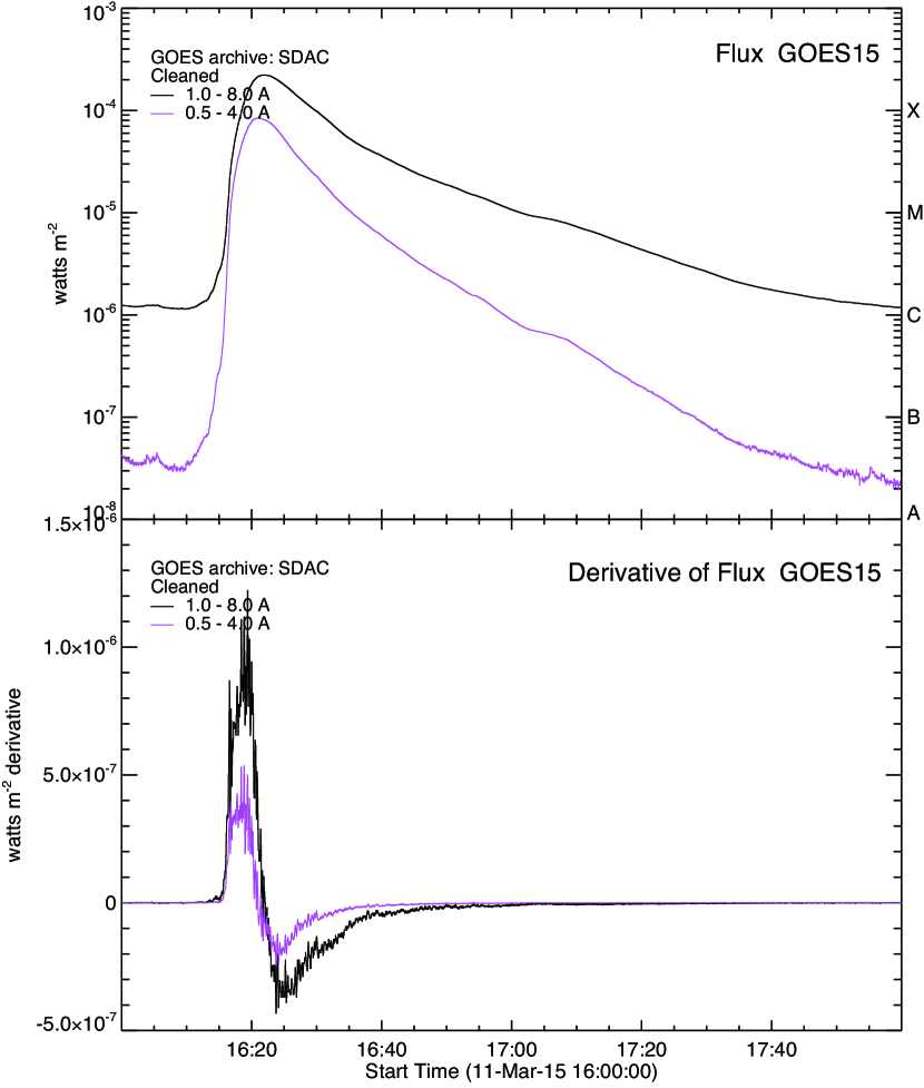
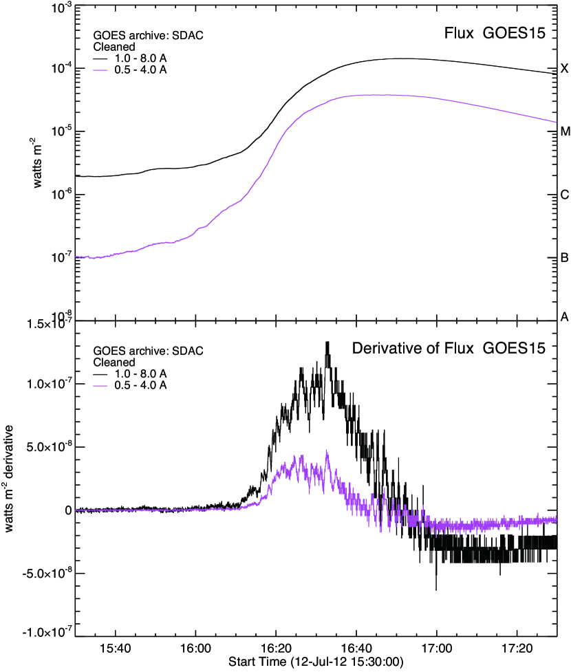
In general, WL enhancements were found to be associated with large flares. However, some NWL events are associated with X-class flares. From these observational facts, it can be inferred that WLFs are associated with impulsive flares. Using this inference, correlations with flare duration were sought. The soft X-ray duration is easily obtained from GOES flare information (GOES flare start to end time). However, some flares occurred consecutively over a short time period and it was not possible to identify the start time and/or end time from soft X-ray light curves. It was therefore decided to use soft X-ray derivative data in order determine flare duration. The soft X-ray derivative profile is almost the same as the hard X-ray profile from the Neupert effect (Neupert, 1968). Although the Neupert effect is not always present for all flare events, this relationship was employed in this study because it is a very good index of flare duration.

Figure 1 shows sample light curves of GOES soft X-ray flux and their time derivative. The left panels show an X2.1-class flare on 2015 March 11 as a sample of impulsive flare. The right panels show an X1.4-class flare on 2012 July 12 as a sample of long duration event. Flare duration for the X1.4 flare was four times longer than that of the X2.1 flare. From these soft X-ray derivative data, the derivative start, peak, and end time and derivative duration were obtained, as shown in Tables 1 and 3. The derivative peak time is defined as the time of the peak in derivative data from the start of the GOES flare to its peak. The derivative start time is defined as the time when the derivative data has a continuous positive value till the derivative peak. The derivative end time is defined as the time from the first negative value from the derivative peak time. In some events (flares on June 13, 2012, December 05, 2014, and 15 March 2015), no GOES data could be obtained and so no derivative data information appears in Tables 1 and 3.

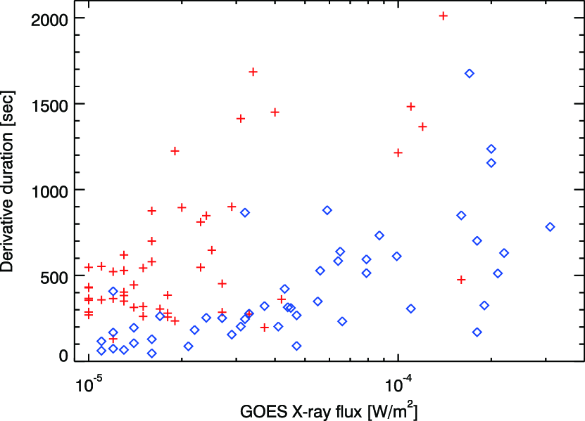
The relationship between the GOES soft X-ray peak flux and the derivative duration is shown in the left-hand side panel of Figure 2. WLF events (represented by blue diamonds) show shorter duration compared with NWL events (represented by red crosses). It appears that the flare derivative duration is roughly correlated with the GOES soft X-ray flux. As a result, the average of both groups could not be compared directly. The average duration of WLF events was $419~{}{\rm s}$ , whereas the average duration for NWL events was $619~{}{\rm s}$ . The average duration of NWL events is therefore $1.5$ times longer than that of WLF events.

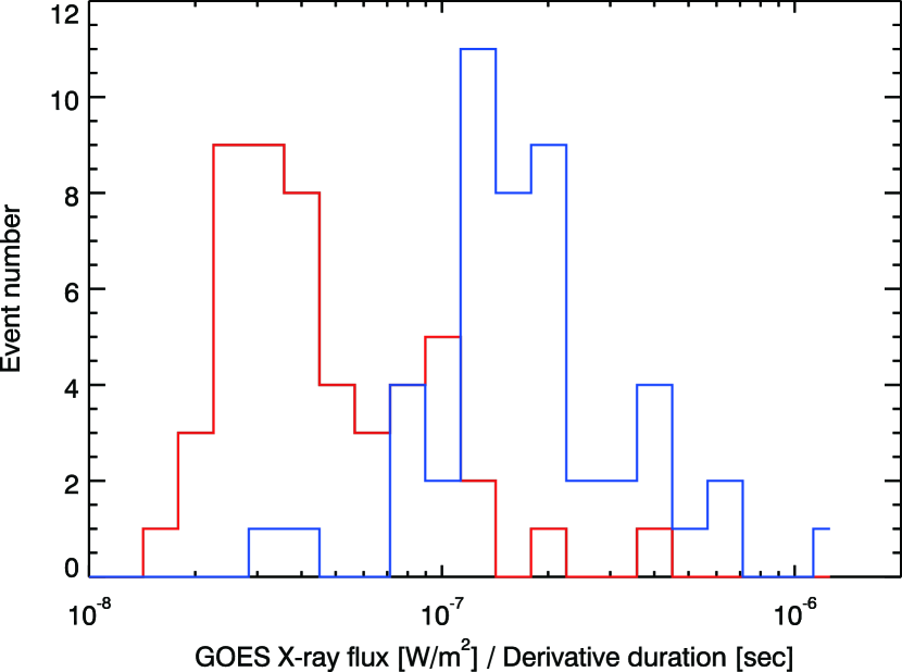
Because there is a relationship between the GOES X-ray peak flux and the flare derivative duration, the GOES X-ray peak flux was divided by the derivative duration and this number was used to represent the impulsivity of the flare. This impulsivity reflects the increase in rate of hard X-ray emission. If there are RHESSI data for all flare events, we don’t need to use the GOES X-ray derivative data, only the one third of flare events were observed by RHESSI in fact. So, we used this method. The right-hand side panel of Figure 2 shows a histogram of flare impulsivity. Figure 2 clearly shows two separate peaks, namely, WLF events (blue), which exhibit a shorter duration and larger flare class (impulsive flare) compared with NWL events (red). This result indicates that the impulsivity of the flare is one of the causative factors of WL enhancement.

3.2 Temperature and Emission Measure

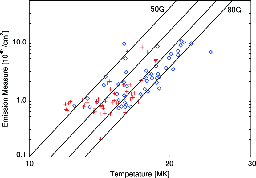
The temperature and emission measure of each flare was calculated using the CHIANTI model. These values were measured at the derivative end time because this time characterizes the end of the energy release from the flare. Figure 3 is a scatter plot of the temperature and emission measure for all events and this graphically indicates there is a positive correlation between these two parameters. The relationship between the emission measure and electron temperature has been reported by Shibata & Yokoyama (1999, 2002). Fig. 2 in Shibata & Yokoyama (2002) shows four theoretical curves for coronal magnetic field strengths of $5$ , $15$ , $50$ , and $150~{}{\rm G}$ at the energy-release site of the flare. When this figure is compared with Figure 3 presented in this study, it can be observed that WLF and NWL events are located within the solar flare region. It can be seen that WLF events (represented by blue diamonds) are distributed toward the right-hand side of the plot, whereas NWL events (represented by red crosses) are located on the left-hand side of the plot. Four theoretical curves with magnetic field strength $B=50,60,70,80~{}{\rm G}$ are also plotted in Figure 3. Inspection of the $B=70~{}{\rm G}$ curve indicates that $41$ NWL events ( $82\%$ of the NWL events) are located on the left-hand side of Figure 3 (region of weak coronal magnetic field strength) and $31$ WLF events ( $65\%$ of the WLF events) are located on the right-hand side of Figure 3 (region of strong coronal magnetic field strength). The difference in the distribution of these data may be due to differences in the coronal magnetic field strength at the site of the energy release. This result suggests that there is a tendency of the coronal magnetic field is weaker for NWL events than for WLF events.

3.3 Distance of Flare Ribbons

The distance of flare ribbons is measured in order to obtain the difference between the flare formal size for WLF and NWF events. To determine flare ribbons, the $1600~{}{\rm\AA}$ UV emission of the Atmospheric Imaging Assembly (AIA; Lemen et al., 2012) onboard SDO was used. From the observed two flare ribbons, the brightest point of each ribbon at the corresponding GOES soft X-ray derivative peak time was determined and the separation between the brightest points was calculated. Among all the events listed in Tables 1 and 3, flare ribbon distance for three events could not be determined due to lack of GOES derivative data. Furthermore, limb flares over E60 or W60 were removed from this analysis. The SDO data for the September 28, 2011 event were found to be missing and so these data were also not included in this analysis. Data were corrected for the effect of parallax in order to determine flare location.

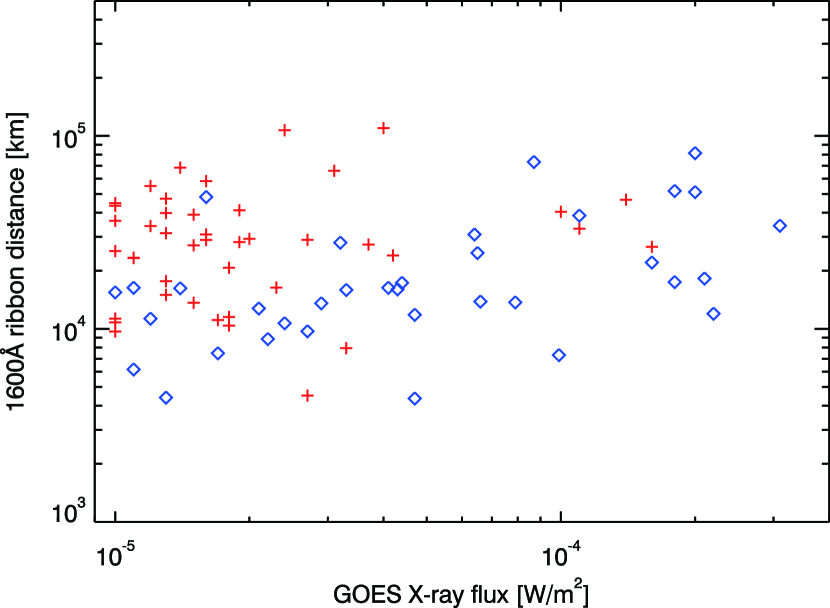
The left-hand side panel of Figure 4 shows the relationship between the separation of the two flare ribbons and GOES soft X-ray class. It appears that there is a rough correlation between the ribbon distance and soft X-ray class, i.e., intense flares have a relatively large size. However, the ribbon distance of NWL events is located in the upper part of the left-hand side panel of Figure 4 compared with that of WLF events. The average separation for WLF events was determined as $2.2\times 10^{3}~{}{\rm km}$ and that for NWL events as $3.3\times 10^{3}~{}{\rm km}$ . The separation of WLF events is therefore significantly less than that of NWL events. This result indicates that the flare formal size of WLF events is relatively more compact than that of NWL events.

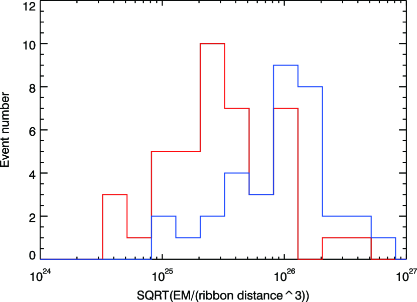
This flare ribbon distance is an index of flare size. When the emission measure is divided by flare volume (distance³) and the square-root taken, an index of flare loop density can be obtained. The right-hand side panel of Figure 4 shows the histogram of event number for flare density. In this figure, it is just possible to see two peaks for WLF events (blue) and for NWL events (red). This result indicates that the plasma density of the flare is one of the causative factors of WL enhancement.

3.4 Field Strength Under the Flare Ribbons

From Section 3.2, it was suggested that there is a relationship between WLF and NWL events and the coronal magnetic field strength. However, no coronal magnetic field strength data exist in the observational data used in this study. Instead, the photospheric magnetic field strength under the flare ribbons as obtained in Section 3.3 is employed.

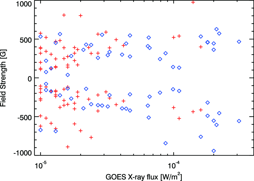
The SDO/HMI field strength data under the $1600~{}{\rm\AA}$ flare ribbons is therefore used in this analysis. For the two flare ribbons associated with each flare, positive field strength is taken from one flare ribbon and negative field strength taken from the other ribbon. Most of the event, these flare ribbons were located on plage region, not umbrae. We calculated the average field strength under the $1600~{}{\rm\AA}$ flare ribbons.

Figure 5 shows the relationship between the GOES soft X-ray peak flux and the field strength under the $1600~{}{\rm\AA}$ flare ribbons as estimated from SDO/HMI data (taken from around the derivative peak time of GOES soft X-ray data). Unfortunately there was a high degree of scatter in the data and no relationship could be determined between these two parameters.

3.5 Hard X-ray Data Analysis

As mentioned in Section 2, a statistical analysis of hard X-ray data as observed by RHESSI was performed. Among the $101$ Hinode/SOT events, $46$ flare events were simultaneously observed with RHESSI. Among the $46$ flare events, $21$ events were associated with the WLF events and $25$ events were the result of NWL events. Among them, $17$ WLF events ( $6$ X-class and $11$ M-class flares) and $10$ NWL events ( $2$ X-class and $9$ M-class flares) have emission greater than $50~{}{\rm keV}$ . Physical parameters for these events are given in Table 3. Based on these events, hard X-ray photon counts and spectra could be analyzed.

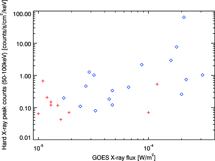
3.5.1 Maximum Photon Counts of Hard X-rays

The maximum photon count of $50-100~{}{\rm keV}$ hard X-ray photons during the flares was investigated. The photon count of each flare is given in Table 3. A scatter plot of the photon count and GOES soft X-ray flux is shown in Figure 6. Consideration of Figure 6 shows that hard X-ray photon count is roughly correlated with the GOES soft X-ray flux. The average photon count of the hard X-rays was calculated and found to be approximately $4.6~{}{\rm counts/s/cm^{2}/keV}$ for WLF events and $0.2~{}{\rm counts/s/cm^{2}/keV}$ for NWL events. Although the standard deviation is larger than the above mentioned values, the maximum photon count of WLF events is significantly larger than that of NWL events. This is directly related to the fact that the GOES soft X-ray flux for WLF events is larger than that for NWL events.

3.5.2 Hard X-ray Spectra and Non-thermal Energy

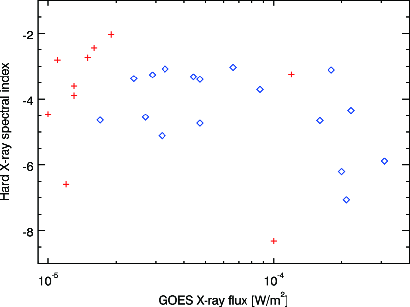
Spectral fitting was performed for $27$ events using a single power law to describe each hard X-ray spectrum in the region of the hard X-ray peak time and in the range of $30-100~{}{\rm keV}$ . Indices for the power laws obtained are given in Table 3 and the correlation of spectral index and GOES soft X-ray flux are given in Figure 7. The average power-law indices are $-4.3$ for WLF events and $-4.0$ for NWL events. Because the standard deviation is smaller than $-1.0$ , there is no significant difference in the power-law indices.

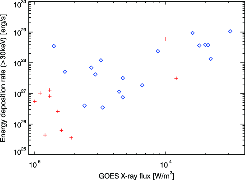
The deposition rate of non-thermal energy was then calculated assuming a thick target model with a low-energy cutoff of $30~{}{\rm keV}$ (Brown,, 1971). This was done using the same method as described in (Watanabe et al., 2010). The calculated deposition rate of the non-thermal energy and GOES soft X-ray flux are given in Table 3. The corresponding scatter plot is found in Figure 8. There is one NWL event in Figure 8 with very high energy deposition. That is the X1.0-class flare on 2014 October 25, and that is due to the very soft power index for this event. The average deposition rate of non-thermal energy was found to be $2.34\pm 3.05\times 10^{28}~{}{\rm erg/s}$ for WLF events and $6.68\pm 1.77\times 10^{27}~{}{\rm erg/s}$ for NWL events. The deposition rate of WLF events is significantly larger than that of NWL events and this is because the GOES soft X-ray flux for WLF events is larger than that for NWL events.

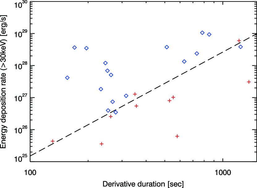
The X-axis from the GOES soft X-ray flux is then plotted as the derivative duration, and the results are shown in Figure 9. In Figure 9, WLF events are located on the upper left-hand side of the dashed line and NWL evens are located on the lower right-hand side of the dashed line. It is important to note that these data occupy separate regimes in Figure 9. This result suggests that the injection rate of non-thermal electrons is one of the causative factors of WL enhancement.

4 Discussion

The results described in the previous sections can be summarized as follows:

(1)

The derivative duration of GOES soft X-rays during WLF events is relatively short.
(2)

WLF events are characterized by stronger magnetic fields at the energy-release site compared with NWL events from the relationship between the temperature and emission measure.
(3)

The separation between two ribbons is shorter for WLF events.
(4)

No significant difference exists in field strength under the flare ribbons.
(5)

The hard X-ray photon count in the energy range of $50-100~{}{\rm keV}$ and the deposition rate of non-thermal energy ( $>30~{}{\rm keV}$ ) are correlated with the GOES soft X-ray flux.
(6)

No significant difference exists between the power-law indices of hard X-ray spectra for WLF and NWL events.
(7)

WLF events are characterized by larger deposition rates of non-thermal energy compared with NWL events. WLF events are characterized by a shorter derivative duration for a given deposition rate.

From results (1) and (3), WLF events appear to be small in terms of spatial extent and have a relatively short duration. WLF events are therefore short-lived and exhibit a rapid enhancement phase, whereas NWL events show a gradual enhancement phase. The short separation of flare ribbons implies that the magnetic field structure related to WLF events is compact. During the evolution of a flare, the separation between flare ribbons increases as a function of time, which is consistent with the short duration. Result (3) suggests that the magnetic loop related to WLF events occurs at low altitudes. In general, the magnetic field is stronger at low altitudes than at high altitudes. The energy release of WLF events therefore appears to occur in the lower corona wherein the magnetic field is relatively strong.

Result (2) suggests the existence of strong magnetic fields at the energy-release site for WLF events. The scatter plot of the emission measure and electron temperature reported in Fig. 2 of Shibata & Yokoyama (2002) shows four theoretical curves for coronal magnetic field strengths of $5$ , $15$ , $50$ , and $150~{}{\rm G}$ at the energy-release site of the flare. The scatter plot of emission measure and electron temperature reported in this investigation (Fig. 2) shows that WLF events are distributed toward the right-hand side of plot, whereas NWL events are located on the left-hand side of the plot. The difference in the distribution of these data may be due to differences in coronal magnetic field strength at the energy-release site. The magnetic field is weaker for NWL events than for WLF events. This finding is consistent with result (3) as the magnetic field is stronger at lower altitudes in the corona.

An attempt was made to check the field strength of the photosphere. However, due to lack of field strength data at the energy-release site, an alternative analysis was undertaken, as described in Section 3.4. No significant difference was observed in the field strength under the flare ribbons.

Results (5) to (7) relate to the hard X-ray observations. As described in Section 1, WL enhancement is correlated with hard X-ray sources in time, location, and energy. Contrary to the expectations of this study, no significant difference was observed in the power-law indices of WLF and NWL events. It therefore follows that the energy distribution of accelerated electrons is similar in both WLF and NWL events. Only very high-energy ( $\gg 100~{}{\rm keV}$ ) electrons can reach the photosphere (Aboudarham & Henoux, 1986; Neidig, 1989). Results presented in this work do not show that the fraction of electrons with such high energies is larger in WLF events compared with NWL events. This result does not support the model whereby electrons penetrate directly into the photosphere and emit WL. However, as the conclusions presented here are the result of a statistical analysis, it is possible that some WLF events may result from this process.

The results presented in this investigation indicate that in order to enhance WL emissions, a large number of accelerated electrons must precipitate within a short period, thereby leading to very rapid heating of the atmosphere. Result (7) suggests that rapid heating is important and that a threshold exists in terms of the injection rate of non-thermal electrons required to generate WL emission.

Through this statistical study, it has been shown that WLF events are characterized by stronger magnetic fields at the energy-release site compared with NWL events. This strong magnetic field may be a factor in the enhancement of WL emission. It is important to consider how a strong magnetic field may be related to WLF events. Two models explain WL emission and indicate that the energy-release region is characterized by a strong magnetic field. In the solar flare model based on magnetic reconnection, the energy-release rate increases if the energy-release region has a strong magnetic field and electrons are accelerated. Hard X-ray sources appear at the region wherein the magnetic field is strongest along the flare ribbon (Asai et al., 2002). Large numbers of electrons are accelerated and this leads to the enhancement of WL emission. The strong magnetic field may also be considered in terms of the trapping efficiency of accelerated electrons in the flare loop. If the top part of the loop is characterized by a stronger magnetic field than that of the foot-point region, the magnetic mirror ratio between the top and the foot-point becomes small and the loss-cone angle is large. Because of this effect, a larger number of accelerated electrons can precipitate into the foot-point region within a short period of time. The trapping efficiency of the loop is therefore lower and most of the accelerated electrons precipitate directly into the foot-point region. This scenario is consistent with results obtained in this study.

Investigating the magnetic structure of a flare region could prove interesting and may reveal how and why the magnetic field strength at the energy-release site is related to the generation mechanism of WLF events.

5 Conclusion

A statistical study has been presented comprising $101$ solar flares observed using the visible continuum filter of Hinode/SOT and SDO/HMI for GOES M- and X-class flares occurring during the period from January 2011 to February 2016. Of these $101$ events, $49$ WLF events and $52$ NWL events were identified on the basis of the existence of an enhancement of the visible continuum images obtained using Hinode/SOT and SDO/HMI. The WLF events are characterized by short duration, a high temperature in the GOES soft X-ray data, and short distance between two flare ribbons in the SDO/AIA $1600~{}{\rm\AA}$ observations. No significant difference was observed between WLF and NWL events in terms of power-law indices, flux of non-thermal photons ( $50-100~{}{\rm keV}$ ), or in the deposition rate of the non-thermal energy. However, a clear relationship between the injection rate of non-thermal energy and derivative duration was observed. These results indicate that during WLF events, accelerated electrons precipitate in a short time period, thereby leading to rapid heating of the atmosphere. The similarity in the power-law index of hard X-ray spectra, as well as the similar deposition rate of non-thermal energy, does not indicate that the fraction of electrons with very high energies ( $\gg 100~{}{\rm keV}$ ) is larger in WLF events compared with NWL events. Relatively low-energy ( $<100~{}{\rm keV}$ ) electrons appear to contribute to the enhancement of WL. This finding is consistent with studies detailing the energy budget between non-thermal electrons and WL emission (Watanabe et al., 2010).

The statistical analysis presented here suggests that the non-thermal energy deposition rate and the magnetic field strength at the energy-release site are significant in WL emission in solar flares. In future work, investigating the magnetic field structure around the energy-release site would be interesting to describe more fully the environment of non-thermal electrons. The physical relationship between the magnetic field structure and the energy of electrons should therefore be the subject of a detailed investigation. Such a study would be expected to provide insight into not only the process of WL emission but also into the acceleration of electrons in solar flares.

It is useful to derive the color temperature of WLF when its energy source is studied (Watanabe et al., 2013; Kerr & Fletcher, 2014). However, we didn’t derive it in this paper because we focused on the difference of WLF and NWL events. In future, we would like to perform this kind of detailed WLF analyses which would provide unique constraints for radiative-hydrodynamic flare models and might reveal lower atmospheric heating differences in impulsive flares and non-impulsive flares. Moreover, Kowalski et al. (2013) showd how the NUV and optical continuum spectral properties of M dwarf flares vary from impulsive flare events to gradual flare events, where the type of flare (impulsive vs. gradual) is determined from a similar quantity as the ”impulsivity”. It would also be interesting to discuss how their results for M dwarf WLFs connect with our study.

Hinode is a Japanese mission developed and launched by ISAS/JAXA, with NAOJ as domestic partner and NASA and STFC (UK) as international partners. It is operated by these agencies in co-operation with ESA and NSC (Norway). This study was supported by the JSPS KAKENHI Grant Numbers JP15K17622, JP16H01187. This work was performed by the joint research program of the Institute for Space-Earth Environmental Research (ISEE), Nagoya University.

References

Aboudarham & Henoux (1986) Aboudarham, J. & Henoux J. C. 1986, A&A, 156, 73
Asai et al. (2002) Asai, A., Masuda, S., Yokoyama, T., et al. 2002, ApJ, 578, L91
Battaglia & Kontar (2011) Battaglia, M. & Kontar, E. P. 2011, A&A, 533, L2
Battaglia & Kontar (2012) Battaglia, M. & Kontar, E. P. 2012, ApJ, 760, 2, 142
Brown, (1971) Brown, J. C., Sol. Phys., 18, 489
Carrington (1859) Carrington,1859, MNRAS, 20, 13
Ding et al. (2003) Ding, M. D., Liu, Y., Yeh, C.-T., Li, J. P. 2003, A&A, 403, 1151
Fletcher et al. (2007) Fletcher, L., Hannah, I. G., Hudson, H. S., and Metcalf, T. R. 2007, ApJ, 656, 2, 1187
Golub et al. (2007) Golub, L., DeLuca, E., Austin, G., et al. 2007, Sol. Phys., 243, 1, 63
Hudson et al. (2006) Hudson, H. S., Wolfson, C. J., & Metcalf, T. R. 2006, Sol. Phys., 234, 1, 79
Ichimoto et al. (2008) Ichimoto, K., Lites, B., Elmore, D., et al. 2008, Sol. Phys., 249, 2, 233
Isobe et al. (2007) Isobe, H., Kubo, M., Minoshima, T., et al. 2007, PASJ, 59, SP3, S807
Jess et al. (2008) Jess, D. B., Mathioudakis, M., Crockett, P. J., Keenan, F. P. 2008, ApJ, 688, 2, L119
Kano et al. (2008) Kano, R., Sakao, T., Hara, H., et al. 2008, Sol. Phys., 249, 2, 263
Kerr & Fletcher (2014) Kerr, G. S., & Fletcher, L. 2014, ApJ, 783, 98
Kowalski et al. (2013) Kowalski, Adam F., Hawley, Suzanne L., Wisniewski, John P. et al. 2013, ApJS, 207, 15
Krucker et al. (2011) Krucker, S., Hudson, H. S., Jeffrey, N. L. S. et al. 2011, ApJ, 739, 2, 96
Krucker et al. (2015) Krucker, S., Saint-Hilaire, P., Hudson, H. S. et al. 2015, ApJ, 802, 19
Kuhar et al. (2016) Kuhar, M., Krucker, S., Martínez Oliveros, J.-C., Battaglia, M., Kleint, L. 2016, ApJ, 816:6
Lemen et al. (2012) Lemen, J. R., Title, A. M., Akin, D. J., et al. 2012, Sol. Phys., 275, 17
Lin et al. (2002) Lin, R. P., Dennis, B. R., Hurford, G. J., et al. 2002, Sol. Phys., 210, 1, 3
Machado et al. (1986) Machado, M. E., Avrett, E. H., Falciani, R., et al. 1986, in ’The Lower Atmosphere of Solar Flares’, ed. D. F. Neidig (Sunspot: NSO), 483
Machado et al. (1989) Machado, M. E., Emslie, A. G., & Avrett, E. H. 1989, Sol. Phys., 124, 303
Martínez Oliveros et al. (2012) Martínez Oliveros, J.-C., Hudson, H. S., Hurford, G. J., et al. 2012, ApJ, 753, 2, L26
Matthews et al. (2003) Matthews, S. A., van Driel-Gesztelyi, L., Hudson, H. S., Nitta, N. V. 2003, A&A, 409, 1107
Metcalf et al. (1990) Metcalf, T. R., Canfield, R. C., & Saba, J. L. R. 1990, ApJ, 365, 391
Metcalf et al. (2003) Metcalf, T. R., Alexander, D., Hudson, H. S., Longcope, D. W. 2003, ApJ, 595, 1, 483
Namekata et al. (2017) Namekata, K., Sakaue, T., Watanabe, K., et al. 2017, PASJ, 69, 7
Neupert (1968) Neupert, W., 1968, ApJ, 153, L59
Neidig (1989) Neidig, D. F. 1989, Sol. Phys., 121, 261
Pesnell et al. (2012) Pesnell, W. D., Thompson, B. J., & Chamberlin, P. C. 2012, Sol. Phys., 275, 3
Scherrer et al. (2012) Scherrer, P. H., Schou, J., Bush, R. I., et al. 2012, Sol. Phys., 275, 207
Schou et al. (2012) Schou, J., Scherrer, P. H., Bush, R. I. et al. 2012, Sol. Phys., 275, 229
Shibata & Yokoyama (1999) Shibata, K. & Yokoyama, T. 1999, ApJ, 526, L49
Shibata & Yokoyama (2002) Shibata, K. & Yokoyama, T. 2002, ApJ, 577, 422
Shimizu et al. (2008) Shimizu, T., Nagata, S., Tsuneta, S., et al. 2008, Sol. Phys., 249, 2, 221
Suematsu et al. (2008) Suematsu, Y., Tsuneta, S., Ichimoto, K., et al. 2008, Sol. Phys., 249, 2, 197
Tsuneta et al. (2008) Tsuneta, S., Suematsu, Y., Ichimoto, K., et al. 2008, Sol. Phys., 249, 2, 167
Wang et al. (2009) Wang et al., 2009, Res. Astron. Astrophys., 9, 127
Watanabe et al. (2010) Watanabe, K., Krucker, S., Hudson, H., et al. 2010, ApJ, 715, 1, 651
Watanabe et al. (2012) Watanabe, K., Masuda, S., and Segawa, T. 2012, Sol. Phys., 279, 1, 317
Watanabe et al. (2013) Watanabe, K., Shimizu, T., Masuda, S., et al. 2013, ApJ, 776, 123

Refer to caption — Figure 1: Sample light curves of GOES soft X-ray flux and their derivative of flux. Left: GOES soft X-ray light curve (top) of the X2.1 flare on 2015 March 11 for the sample of impulsive flare and its time derivative (bottom).Right: GOES soft X-ray light curve (top) of the X1.4 flare on 2012 July 12 for the sample of non-impulsive flare and its time derivative (bottom).

\floattable

Table 1: WLF event list and physical parameters from GOES & SDO data.

				GOES		derivative	@derivative end		$1600{\rm\AA}$ ribbon	HMI field strength
GOES flare start	GOES derivative			X-ray	Sunspot	duration	Temperature	EM	distance	@ $1600{\rm\AA}$ ribbon
YYYY/MM/DD hh:mm	start	peak	end	class	location	[sec]	[MK]	[ $10^{49}/{\rm cm}^{3}$ ]	[ $\times 10^{3}{\rm km}$ ]	positive [G]	negative [G]
2011/02/15 01:44	2011/02/15 01:45	2011/02/15 01:52	2011/02/15 01:56	X2.2	S20W10	631	21.3	9.85	12.0	572.4	-455.2
2011/11/03 20:16	2011/11/03 20:17	2011/11/03 20:21	2011/11/03 20:22	X1.9	N21E64	326	20.9	5.68
2012/01/27 17:37	2012/01/27 18:05	2012/01/27 18:26	2012/01/27 18:33	X1.7	N33W85	1676	16.0	8.88
2012/07/06 23:01	2012/07/06 23:03	2012/07/06 23:06	2012/07/06 23:08	X1.1	S13W59	307	20.0	5.07	38.6	131.6	-168.4
2012/10/23 03:13	2012/10/23 03:14	2012/10/23 03:15	2012/10/23 03:16	X1.8	S13E58	170	24.6	6.42	17.5	460.9	-488.9
2014/10/22 14:02	2014/10/22 14:03	2014/10/22 14:15	2014/10/22 14:17	X1.6	S14E13	850	20.2	5.99	22.1	533.8	-759.8
2014/10/24 20:50	2014/10/24 21:06	2014/10/24 21:15	2014/10/24 21:19	X3.1	S16W21	783	22.3	9.00	34.3	466.9	-557.0
2014/10/26 10:04	2014/10/26 10:35	2014/10/26 10:44	2014/10/26 10:54	X2.0	S18W40	1155	21.2	8.41	51.1	443.9	-942.0
2014/10/27 14:12	2014/10/27 14:10	2014/10/27 14:26	2014/10/27 14:31	X2.0	S17W52	1237	20.9	6.72	81.4	363.0	-552.5
2014/12/20 00:11	2014/12/20 00:14	2014/12/20 00:21	2014/12/20 00:25	X1.8	S21W24	702	18.9	8.05	51.8	457.0	-318.8
2015/03/11 16:11	2015/03/11 16:13	2015/03/11 16:19	2015/03/11 16:21	X2.1	S17E22	512	21.5	9.38	18.2	627.8	-606.4
2011/02/14 17:20	2011/02/14 17:23	2011/02/14 17:24	2011/02/14 17:26	M2.2	S20W04	183	15.4	1.22	8.9	429.2	-140.8
2011/02/18 09:55	2011/02/18 10:07	2011/02/18 10:10	2011/02/18 10:11	M6.6	S21W55	233	20.4	3.25	13.8	386.9	-242.4
2011/02/18 12:59	2011/02/18 13:00	2011/02/18 13:02	2011/02/18 13:03	M1.4	S21W55	196	16.2	0.78	16.2	565.5	-225.3
2011/09/28 13:24	2011/09/28 13:25	2011/09/28 13:26	2011/09/28 13:28	M1.2	N11E00	168	15.6	0.69
2011/11/02 21:52	2011/11/02 21:53	2011/11/02 21:57	2011/11/02 22:00	M4.3	N20E77	422	17.9	2.05
2011/12/31 13:09	2011/12/31 13:11	2011/12/31 13:13	2011/12/31 13:15	M2.4	S25E46	254	17.4	1.21	10.7	425.1	-339.9
2012/03/06 12:23	2012/03/06 12:39	2012/03/06 12:40	2012/03/06 12:41	M2.1	N21E40	88	16.0	1.15	12.8	362.1	-392.8
2012/03/06 21:04	2012/03/06 21:09	2012/03/06 21:10	2012/03/06 21:11	M1.3	N16E30	67	16.1	0.73	4.4	451.4	-687.6
2012/05/09 12:21	2012/05/09 12:27	2012/05/09 12:29	2012/05/09 12:32	M4.7	N13E31	268	18.4	2.28	11.8	275.4	-212.2
2012/05/09 21:01	2012/05/09 21:01	2012/05/09 21:03	2012/05/09 21:05	M4.1	N12E26	203	18.8	1.91	16.3	299.9	-393.8
2012/05/10 20:20	2012/05/10 20:21	2012/05/10 20:25	2012/05/10 20:26	M1.7	N12E12	263	15.6	0.95	7.5	282.0	-267.2
2012/07/05 03:25	2012/07/05 03:34	2012/07/05 03:35	2012/07/05 03:36	M4.7	S18W29	90	18.8	2.27	4.4	547.5	-421.1
2012/07/05 21:37	2012/07/05 21:44	2012/07/05 21:45	2012/07/05 21:45	M1.6	S12W46	47	13.4	1.02	48.2	38.3	-136.8
2012/07/06 01:37	2012/07/06 01:37	2012/07/06 01:38	2012/07/06 01:40	M2.9	S18W41	156	17.7	1.46	13.6	556.3	-357.1

\floattable

Table 2: WLF event list and physical parameters from GOES & SDO data. (cont.)

				GOES		derivative	@derivative end		$1600{\rm\AA}$ ribbon	HMI field strength
GOES flare start	GOES derivative			X-ray	Sunspot	duration	Temperature	EM	distance	@ $1600{\rm\AA}$ ribbon
YYYY/MM/DD hh:mm	start	peak	end	class	location	[sec]	[MK]	[ $10^{49}/{\rm cm}^{3}$ ]	[ $\times 10^{3}{\rm km}$ ]	positive [G]	negative [G]
2012/07/08 12:05	2012/07/08 12:08	2012/07/08 12:09	2012/07/08 12:10	M1.4	S21W69	106	16.5	0.73
2013/06/07 22:11	2013/06/07 22:33	2013/06/07 22:43	2013/06/07 22:48	M5.9	S32W89	880	18.9	2.69
2013/10/26 19:24	2013/10/26 19:23	2013/10/26 19:24	2013/10/26 19:27	M3.1	S09E81	203	14.5	1.72
2013/10/28 15:07	2013/10/28 15:09	2013/10/28 15:10	2013/10/28 15:14	M4.4	S06E28	315	14.6	2.39	17.3	443.2	-397.2
2013/12/22 14:45	2013/12/22 15:07	2013/12/22 15:10	2013/12/22 15:12	M3.3	S19W56	278	15.6	1.80	15.9	334.4	-223.1
2013/12/23 08:59	2013/12/23 09:04	2013/12/23 09:06	2013/12/23 09:06	M1.6	S17W63	129	16.1	0.86
2013/12/31 21:45	2013/12/31 21:47	2013/12/31 21:52	2013/12/31 21:57	M6.4	S16W35	584	17.9	3.06	30.9	409.1	-358.2
2014/01/01 18:40	2014/01/01 18:41	2014/01/01 18:47	2014/01/01 18:51	M9.9	S14W47	612	16.1	4.99	7.3	140.5	-147.2
2014/03/13 19:03	2014/03/13 19:10	2014/03/13 19:12	2014/03/13 19:17	M1.2	N15W87	408	13.5	0.72
2014/10/21 13:35	2014/10/21 13:36	2014/10/21 13:37	2014/10/21 13:37	M1.2	S14E35	74	14.0	0.87	11.3	122.7	-174.1
2014/10/22 01:16	2014/10/22 01:36	2014/10/22 01:46	2014/10/22 01:49	M8.7	S13E21	733	19.7	3.41	73.2	317.5	-843.2
2014/11/05 09:26	2014/11/05 09:38	2014/11/05 09:42	2014/11/05 09:46	M7.9	N20E68	514	18.7	3.68
2014/11/15 11:40	2014/11/15 11:48	2014/11/15 11:58	2014/11/15 12:02	M3.2	S09E63	866	16.2	1.65
2014/11/15 20:38	2014/11/15 20:40	2014/11/15 20:43	2014/11/15 20:45	M3.7	S13E63	322	16.0	1.93
2015/01/13 04:13	2015/01/13 04:15	2015/01/13 04:21	2015/01/13 04:24	M5.6	N06W70	528	16.2	2.89
2015/03/12 04:41	2015/03/12 04:41	2015/03/12 04:43	2015/03/12 04:45	M3.2	S15E11	246	19.0	1.51	28.0	292.4	-369.0
2015/03/12 21:44	2015/03/12 21:46	2015/03/12 21:48	2015/03/12 21:50	M2.7	S15E01	252	18.0	1.34	9.7	258.2	-352.4
2015/03/15 09:36				M1.0	S20W24
2015/06/22 17:23	2015/06/22 17:49	2015/06/22 17:58	2015/06/22 18:00	M6.5	N12W08	639	19.1	2.38	24.7	520.0	-511.8
2015/06/25 08:02	2015/06/25 08:04	2015/06/25 08:14	2015/06/25 08:14	M7.9	N09W42	594	18.3	2.66	13.7	242.7	-190.5
2015/09/29 19:08	2015/09/29 19:22	2015/09/29 19:23	2015/09/29 19:24	M1.1	S20W36	117	12.5	0.76	16.3	75.5	-77.8
2015/09/30 13:14	2015/09/30 13:18	2015/09/30 13:19	2015/09/30 13:20	M1.1	S23W59	62	15.8	0.74	6.2	221.2	-156.9
2015/10/01 13:03	2015/10/01 13:05	2015/10/01 13:09	2015/10/01 13:10	M4.5	S23W64	311	17.9	2.27
2015/10/02 00:06	2015/10/02 00:07	2015/10/02 00:10	2015/10/02 00:13	M5.5	S19W67	349	18.1	2.71

\floattable

Table 3: NWL event list and physical parameters from GOES & SDO data.

				GOES		derivative	@derivative end		$1600{\rm\AA}$ ribbon	HMI field strength
GOES flare start	GOES derivative			X-ray	Sunspot	duration	Temperature	EM	distance	@ $1600{\rm\AA}$ ribbon
YYYY/MM/DD hh:mm	start	peak	end	class	location	[sec]	[MK]	[ $10^{49}/{\rm cm}^{3}$ ]	[ $\times 10^{3}{\rm km}$ ]	positive [G]	negative [G]
2012/03/05 02:30	2012/03/05 03:30	2012/03/05 03:45	2012/03/05 03:55	X1.1	N19E58	1483	18.7	4.55	33.0	539.2	-523.3
2012/07/12 15:37	2012/07/12 16:11	2012/07/12 16:32	2012/07/12 16:44	X1.4	S13W03	2011	17.9	6.47	46.7	975.8	-436.5
2013/05/15 01:24	2013/05/15 01:25	2013/05/15 01:43	2013/05/15 01:48	X1.2	N12E64	1366	16.3	6.57
2014/10/25 16:55	2014/10/25 16:47	2014/10/25 17:03	2014/10/25 17:07	X1.0	S10W22	1214	19.8	4.79	40.4	521.6	-383.5
2014/11/07 16:53	2014/11/07 17:17	2014/11/07 17:22	2014/11/07 17:25	X1.6	N14E36	475	17.5	7.83	26.6	399.4	-413.7
2011/02/16 07:35	2011/02/16 07:37	2011/02/16 07:40	2011/02/16 07:43	M1.1	S19W29	358	16.1	0.58	23.3	521.3	-519.7
2011/09/23 21:54	2011/09/23 21:59	2011/09/23 22:03	2011/09/23 22:10	M1.6	N12E56	700	13.3	0.88	58.2	274.8	-890.5
2011/11/03 10:58	2011/11/03 10:59	2011/11/03 11:07	2011/11/03 11:10	M2.5	N20E70	647	16.8	1.26
2011/11/05 03:08	2011/11/05 03:29	2011/11/05 03:30	2011/11/05 03:32	M3.7	N20E47	197	14.9	2.00	27.3	492.4	-345.4
2011/11/05 20:31	2011/11/05 20:33	2011/11/05 20:35	2011/11/05 20:37	M1.8	N21E37	258	17.2	0.89	11.5	391.1	-327.5
2011/12/31 16:16	2011/12/31 16:21	2011/12/31 16:24	2011/12/31 16:25	M1.5	S25E42	262	15.6	0.85	27.1	248.6	-353.7
2012/01/17 04:41	2012/01/17 04:43	2012/01/17 04:45	2012/01/17 04:52	M1.0	N18E53	547	13.8	0.59	11.3	199.2	-140.5
2012/01/18 19:04	2012/01/18 19:06	2012/01/18 19:09	2012/01/18 19:11	M1.7	N17E32	305	14.6	0.91	11.1
2012/05/07 14:03	2012/05/07 14:05	2012/05/07 14:19	2012/05/07 14:26	M1.9	S20W49	1224	14.1	1.00	41.1	166.8	-241.4
2012/05/09 14:02	2012/05/09 14:04	2012/05/09 14:06	2012/05/09 14:08	M1.8	N06E22	280	14.8	1.04	20.7	223.2	-594.1
2012/06/13 11:29				M1.2	S16E18
2012/07/06 08:17	2012/07/06 08:18	2012/07/06 08:22	2012/07/06 08:23	M1.5	S17W40	319	15.4	0.84	13.7	809.5	-291.3
2012/07/14 04:51	2012/07/14 04:51	2012/07/14 04:54	2012/07/14 04:58	M1.0	S22W36	366	13.8	0.59	44.8	575.1	-623.0
2013/05/02 04:58	2013/05/02 04:59	2013/05/02 05:04	2013/05/02 05:08	M1.1	N10W26	553	13.8	0.61	23.4	341.9	-116.9
2013/05/03 16:39	2013/05/03 16:40	2013/05/03 16:46	2013/05/03 16:49	M1.3	N10W38	529	13.1	0.72	15.0	140.5	-166.1
2013/08/17 18:16	2013/08/17 18:19	2013/08/17 18:22	2013/08/17 18:23	M3.3	S07W30	275	16.5	1.74	7.9	386.8	-260.6
2013/10/22 00:14	2013/10/22 00:15	2013/10/22 00:18	2013/10/22 00:21	M1.0	N06E17	356	15.0	0.55	25.3	390.9	-490.7
2013/10/28 14:46	2013/10/28 14:55	2013/10/28 14:59	2013/10/28 15:00	M2.7	S08E28	286	16.6	1.22	4.5	318.6	-221.2
2013/12/07 07:17	2013/12/07 07:19	2013/12/07 07:22	2013/12/07 07:28	M1.2	S16W49	522	12.0	0.81	34.1	117.2	-171.1
2013/12/22 08:05	2013/12/22 08:07	2013/12/22 08:09	2013/12/22 08:11	M1.9	S20W49	235	16.5	0.99	28.2	365.2	-183.4

\floattable

Table 4: NWL event list and physical parameters from GOES & SDO data. (cont.)

				GOES		derivative	@derivative end		$1600{\rm\AA}$ ribbon	HMI field strength
GOES flare start	GOES derivative			X-ray	Sunspot	duration	Temperature	EM	distance	@ $1600{\rm\AA}$ ribbon
YYYY/MM/DD hh:mm	start	peak	end	class	location	[sec]	[MK]	[ $10^{49}/{\rm cm}^{3}$ ]	[ $\times 10^{3}{\rm km}$ ]	positive [G]	negative [G]
2014/01/04 10:16	2014/01/04 10:18	2014/01/04 10:20	2014/01/04 10:24	M1.3	S05E48	350	14.2	0.74	47.3	136.1	-240.2
2014/01/04 19:05	2014/01/04 19:04	2014/01/04 19:15	2014/01/04 19:28	M4.0	S11E34	1450	14.7	1.87	109.7
2014/02/14 02:40	2014/02/14 02:47	2014/02/14 02:54	2014/02/14 02:56	M2.3	S12W25	547	15.3	1.24	16.4	390.8	-275.7
2014/02/14 12:29	2014/02/14 12:30	2014/02/14 12:39	2014/02/14 12:40	M1.6	S15W36	580	14.0	0.91	30.9	138.5	-118.4
2014/06/12 21:34	2014/06/12 21:40	2014/06/12 21:57	2014/06/12 22:03	M3.1	S20W55	1413	13.7	1.37	65.9	589.9	-180.8
2014/06/15 23:50	2014/06/15 23:52	2014/06/15 23:56	2014/06/15 23:59	M1.0	S19E08	432	12.1	0.62	36.3	121.8	-187.4
2014/08/01 17:55	2014/08/01 17:56	2014/08/01 18:00	2014/08/01 18:05	M1.5	S10E11	543	12.2	0.84	39.0	388.6	-146.5
2014/10/26 19:59	2014/10/26 19:58	2014/10/26 20:05	2014/10/26 20:12	M2.4	S15W45	848	16.7	1.06	107.0	315.0	-768.5
2014/10/28 02:15	2014/10/28 02:11	2014/10/28 02:37	2014/10/28 02:39	M3.4	S14W61	1685	16.0	1.75
2014/10/29 09:54	2014/10/29 09:55	2014/10/29 09:58	2014/10/29 10:01	M1.2	S18W77	365	14.4	0.69
2014/11/05 18:50	2014/11/05 19:24	2014/11/05 19:31	2014/11/05 19:39	M2.9	N17E65	900	15.0	1.48
2014/11/07 02:01	2014/11/07 02:39	2014/11/07 02:42	2014/11/07 02:46	M2.7	N17E50	452	16.2	1.34	28.9	564.0	-427.6
2014/11/07 09:43	2014/11/07 10:13	2014/11/07 10:17	2014/11/07 10:21	M1.0	N15E43	428	14.3	0.55	9.7	317.4	-267.6
2014/12/04 07:36	2014/12/04 08:01	2014/12/04 08:05	2014/12/04 08:08	M1.3	S24W27	403	13.9	0.69	17.7	470.3	-177.8
2014/12/05 11:33				M1.5	S23W41
2014/12/19 09:31	2014/12/19 09:33	2014/12/19 09:39	2014/12/19 09:43	M1.3	S19W27	619	13.1	0.79	31.3	244.1	-219.3
2015/03/12 12:09	2015/03/12 12:08	2015/03/12 12:11	2015/03/12 12:13	M1.4	S18E05	314	12.3	0.90	68.5	481.5	-380.5
2015/03/12 13:45	2015/03/12 14:02	2015/03/12 14:04	2015/03/12 14:08	M4.2	S15E06	361	17.4	2.07	24.0	417.0	-298.8
2015/03/13 05:49	2015/03/13 06:00	2015/03/13 06:03	2015/03/13 06:07	M1.8	S14W02	385	16.0	0.96	10.4	317.5	-400.0
2015/03/14 04:23	2015/03/14 04:33	2015/03/14 04:36	2015/03/14 04:40	M1.3	S14W12	383	14.4	0.77	39.8	144.4	-655.1
2015/03/15 22:42	2015/03/15 22:45	2015/03/15 22:46	2015/03/15 22:47	M1.2	S19W32	131	14.2	0.20	55.0	304.0	-586.6
2015/03/16 10:39	2015/03/16 10:41	2015/03/16 10:50	2015/03/16 10:56	M1.6	S17W39	876	15.1	0.86	28.9	165.5	-342.2
2015/03/17 22:49	2015/03/17 23:28	2015/03/17 23:30	2015/03/17 23:32	M1.0	S21W56	270	12.0	0.66	43.4	107.7	-106.4
2015/06/21 01:02	2015/06/21 01:22	2015/06/21 01:27	2015/06/21 01:37	M2.0	N12E13	895	15.2	0.94	29.3	803.1	-681.8
2015/08/30 02:01	2015/08/30 02:54	2015/08/30 02:56	2015/08/30 03:01	M1.4	S17W80	445	13.9	0.61
2015/09/27 20:54	2015/09/27 20:55	2015/09/27 20:57	2015/09/27 21:00	M1.0	S21W16	287	14.6	0.57	10.8	378.9	-286.7
2016/01/01 23:10	2016/01/01 23:30	2016/01/01 23:37	2016/01/01 23:44	M2.3	S25W82	811	13.0	0.95

Table 3: WLF & NWL event list and physical parameters from RHESSI data.

GOES flare start	GOES	Sunspot	Derivative	$50-100~{}{\rm keV}$ HXR peak	Power law	Energy deposition rate
YYYY/MM/DD hh:mm	X-ray class	location	duration [s]	[ ${\rm counts/s/cm^{2}/keV}$ ]	index	( $>30~{}{\rm keV}$ ) [erg/s]
NWL events
2013/05/15 01:24	X1.2	N12E64	1366	0.53	-3.2	3.09E+27
2014/10/25 16:55	X1.0	S10W22	1214	0.07	-8.3	5.97E+28
2011/12/31 16:16	M1.5	S25E42	262	0.12	-2.7	2.56E+26
2013/05/02 04:58	M1.1	N10W26	553	0.67	-2.8	1.02E+27
2013/05/03 16:39	M1.3	N10W38	529	0.12	-3.9	8.04E+26
2013/10/22 00:14	M1.0	N06E17	356	0.06	-4.5	5.46E+26
2013/12/22 08:05	M1.9	S20W49	235	0.07	-2.0	3.58E+25
2014/01/04 10:16	M1.3	S05E48	350	0.15	-3.6	1.28E+27
2014/02/14 12:29	M1.6	S15W36	580	0.04	-2.4	6.20E+25
2015/03/15 22:42	M1.2	S19W32	131	0.21	-6.6	4.35E+25
WLF events
2011/02/15 01:44	X2.2	S20W10	631	0.74	-4.3	1.34E+28
2012/10/23 03:13	X1.8	S13E58	170	7.67	-3.1	3.66E+28
2014/10/22 14:02	X1.6	S14E13	850	2.93	-4.7	9.36E+28
2014/10/24 20:50	X3.1	S16W21	783	1.03	-5.9	1.06E+29
2014/10/27 14:12	X2.0	S17W52	1237	0.26	-6.2	3.85E+28
2015/03/11 16:11	X2.1	S17E22	512	64.2	-7.1	3.77E+28
2011/02/18 09:55	M6.6	S21W55	233	0.43	-3.0	1.84E+27
2011/12/31 13:09	M2.4	S25E46	254	0.11	-3.4	3.97E+26
2012/05/09 12:21	M4.7	N13E31	268	0.12	-3.4	7.44E+26
2012/05/10 20:20	M1.7	N12E12	263	0.20	-4.6	5.10E+27
2012/07/05 03:25	M4.7	S18W29	90	0.34	-4.7	3.16E+27
2012/07/06 01:37	M2.9	S18W41	156	1.27	-3.3	4.18E+27
2013/10/28 15:07	M4.4	S06E28	315	0.18	-3.3	1.14E+27
2013/12/22 14:45	M3.3	S19W56	278	0.08	-3.1	3.47E+26
2014/10/22 01:16	M8.7	S13E21	733	2.15	-3.7	2.38E+28
2015/03/12 04:41	M3.2	S15E11	246	1.02	-5.1	1.20E+28
2015/03/12 21:44	M2.7	S15E01	252	0.47	-4.5	6.92E+27