MNRAS LaTeX 2ε template – title goes here

Gravity or turbulence? IV. Collapsing cores in out-of-virial disguise

Abstract

We study the dynamical state of cores by using a simple analytical model, a sample of observational massive cores, and numerical simulations of collapsing massive cores. From the analytical model, we find that, if cores are formed from turbulent compressions, they evolve from small to large column densities, increasing their velocity dispersion as they collapse. This results in a time evolution path in the Larson velocity dispersion-size diagram from large sizes and small velocity dispersions to small sizes and large velocity dispersions, while they tend to equipartition between gravity and kinetic energy.

From the observational sample, we find that: (a) cores with substantially different column densities in the sample do not follow a Larson-like linewidth-size relation. Instead, cores with higher column densities tend to be located in the upper-left corner of the Larson velocity dispersion $\sigma_{{\rm v,3D}}$-size $R$ diagram, a result predicted previously (Ballesteros-Paredes et al., 2011a). (b) The data exhibit cores with overvirial values.

Finally, in the simulations of collapsing cores we reproduce the behavior predicted by the analytical model and depicted in the observational sample: cores evolve towards larger velocity dispersions and smaller sizes as they collapse and increase their column density. More importantly, however, is that collapsing cores appear to approach overvirial states within a free-fall time. We find that the cause of this apparent excess of kinetic energy is an underestimation of the actual gravitational energy, due to the assumption that the gravitational energy is given by the energy of an isolated sphere of constant column density. We find that this apparent excess disappears when the gravitational energy is correctly calculated from the actual spatial mass distribution, where inhomogeneities, as well as the potential due to the mass outside of the core, also contribute to the gravitational energy. We conclude that the observed energy budget of cores in recent surveys is consistent with their non-thermal motions being driven by their self-gravity and in the process of dynamical collapse.

Accepted date. Received date; in original form date

1 Introduction

Since the first detections of molecular gas, it was recognized that their line profiles exhibit supersonic widths (Wilson et al. 1970). Early models interpreting such profiles suggested that they were the signature of clouds in a state of large-scale collapse, since turbulence should decay over a dynamical crossing time (Goldreich & Kwan, 1974; Liszt et al., 1974). This proposal was rapidly dismissed by Zuckerman & Palmer (1974), who argued that the star formation rates would be too large if clouds were in a state of free-fall. These authors proposed, instead, that the supersonic linewidths were produced by small-scale turbulence, which furthermore, might provide support to molecular clouds (MCs) against their own collapse (see, e.g., Vázquez-Semadeni et al., 2000; Mac Low & Klessen, 2004; Ballesteros-Paredes et al., 2007; McKee & Ostriker, 2007; Klessen & Glover, 2016, and references therein).

Indeed, there is a number of apparently good reasons to believe that turbulence may play an important role in the structure and dynamics of MCs. First, the Reynolds numbers in the interestellar medium are very large, indicating that the velocity field should be strongly turbulent (Elmegreen & Scalo, 2004). Second, the velocity field in the ISM exhibits a multi-scale nature that extends over several orders of magnitud in size (e.g., Larson, 1981). Third, clouds exhibit a fractal appareance (Falgarone et al., 1991), characteristic of turbulent fluids. Fourth, stellar jets and winds, gravitational chaotic motions of orbiting gas in the galaxy, SN explosions, spiral arm shocks, etc., may be powering the gas of kinetic energy at multiple scales simultaneously (e.g., Norman & Ferrara, 1996). In addition, the large widths of the observed spectral lines indicate that such turbulence should be supersonic, reinforcing the idea that turbulence is intrinsically related to MC structure by shaping, morphing and fragmenting MCs (Ballesteros-Paredes et al., 1999a; Hopkins, 2012). In the prevailing interpretation, MCs are thought to be near virial equilibrium, with perhaps a moderate excess of kinetic energy, such that some external pressure is needed to confine them for several dynamical times (Bertoldi & McKee, 1992; Field et al., 2011; Miville-Deschênes et al., 2016; Leroy et al., 2015). MC turbulence plays a crucial role providing global support against collapse, while promoting local collapse where motions are converging (e.g., Ballesteros-Paredes et al., 1999a; Mac Low & Klessen, 2004; Ballesteros-Paredes, 2006; Ballesteros-Paredes et al., 2007; Hennebelle & Falgarone, 2012; Padoan et al., 2014).

Although the turbulent nature of the velocity field in MCs is hardly questionable, several problems remain with the standard interpretation that it can provide support against the global collapse of the clouds: First, turbulence consists of a hierarchy of coherent motions over a wide range of scales for which the largest-amplitude velocity fluctuations occur at the largest scales. This implies that the dominant MC turbulent motions are far from being the small-scale turbulent motions that can provide the internal turbulent pressure to support the cloud against gravity (see, e.g., Ballesteros-Paredes, 2006), as confirmed numerically by Brunt et al. (2009). Thus, the dominant motions induced by turbulence at the scale of clouds will be cloud-scale motions such as compression, expansion, shearing or rotation, but not thermal-like, small-scale motions that can provide an internal pressure to support it against gravity (see, e.g., Ballesteros-Paredes et al., 1999a; Ballesteros-Paredes, 2006; Vázquez-Semadeni, 2015).

Second, since turbulence is a dissipative phenomenon, it requires constant driving to be maintained. The standard belief is that the turbulent energy is injected by mainly two mechanisms: one, through instabilities occurring during the assembly stage of the clouds (e.g., Vishniac, 1994; Walder & Folini, 2000; Koyama & Inutsuka, 2002; Audit & Hennebelle, 2005; Heitsch et al., 2005; Vázquez-Semadeni et al., 2006; Klessen & Hennebelle, 2010). The other, by stellar feedback via outflows, winds, ionizing radiation or supernova explosions (e.g., Mac Low & Klessen, 2004; Wang et al., 2010; Vázquez-Semadeni et al., 2010; Gatto et al., 2015; Padoan et al., 2016). Regarding the first point, numerical simulations of the formation of MCs from converging flows generally suggest that the turbulence level produced by various instabilities is significantly lower ($\la 20\%$) than the level typically observed in MCs (e.g., Koyama & Inutsuka, 2002; Heitsch et al., 2005; Audit & Hennebelle, 2005; Vázquez-Semadeni et al., 2007, 2010), even with the inclusion of external SN explosions that trigger the compressions which form the clouds (Ibáñez-Mejía et al., 2016), although this is still matter of debate (e.g., Padoan et al., 2016). With respect to the stellar feedback, it is not clear why the energy it injects would cause apparent near virialization of all molecular structures. In fact, numerical simulations suggest quite the opposite: clumps and moderate-mass MCs appear to be readily disrupted by photoionizing radiation or supernova explosions from massive stars, while high-mass MCs are difficult to prevent from collapsing (e.g., Dale et al., 2012, 2013a, 2013b; Colín et al., 2013). Thus, neither of the two mechanisms is likely to produce the observed magnitude of the nonthermal motions in MCs.

On the other hand, in the last decade, numerical simulations of the formation and evolution of molecular clouds have renewed the idea that molecular clouds may be in a state of collapse. These models suggest that their formation from convergent motions in the warm neutral medium (WNM) in the Galaxy (Ballesteros-Paredes et al., 1999a, b) involves a phase transition to the cold neutral medium (CNM; Hennebelle & Pérault, 1999; Koyama & Inutsuka, 2000; Vázquez-Semadeni et al., 2006), and thus the clouds may be formed with masses much larger than their Jeans mass (Hartmann et al., 2001; Vázquez-Semadeni et al., 2007; Heitsch & Hartmann, 2008; Gómez & Vázquez-Semadeni, 2014), implying that they may very well be in a state of large-scale hierarchical and chaotic collapse (Vázquez-Semadeni et al., 2009; Ballesteros-Paredes et al., 2011a).

Note, however, that, contrary to the suggestion by Zuckerman & Palmer (1974), such a state of global collapse does not necessarily imply that the star formation rate will be too large: The initial fragmentation occuring while the cloud is being assembled has the consequence that only very small amounts of mass are deposited in the high density regions that are responsible for the instantaneous rate of star formation in the clouds, as evidenced by the steep negative slope of the column density probability distribution functions of MCs (Kainulainen et al., 2009; Ballesteros-Paredes et al., 2011b; Kritsuk et al., 2011). Having large nonlinear amplitudes, such dense regions complete their collapse much earlier than the whole cloud, causing a spread in the ages of the stellar products (e.g., Zamora-Avilés et al., 2012; Hartmann et al., 2012; Vázquez-Semadeni et al., 2017). This will eventually produce massive stars that will blow strong winds and rapidly ionize the gas, effectively dispersing the nearby dense gas (e.g., Vázquez-Semadeni et al., 2010; Zamora-Avilés et al., 2012; Dale et al., 2012, 2013a, 2013b; Colín et al., 2013; Zamora-Avilés & Vázquez-Semadeni, 2014; Vázquez-Semadeni et al., 2017), shutting off the local star formation episodes by the time only $\sim 10\%$ of the gas has been converted to stars, thus keeping the global star formation rate and efficiency low.

In this scenario, the supersonic nonthermal motions observed in MCs, albeit still turbulent in the sense of having a chaotic component, are dominated by an infall component that occurs at multiple scales, consituting a regime of collapses within collapses (e.g., Vázquez-Semadeni et al., 2009, 2017). This implies that the nonthermal motions are dominated by a convergent component that results from the gravitational contraction, rather than being a fully random velocity field that can provide a pressure gradient capable of opposing the collapse (Vázquez-Semadeni et al., 2008; González-Samaniego et al., 2014). Nevertheless, the chaotic, moderately-supersonic nature of the truly turbulent motions does produce a spectrum of density fluctuations that provide the focusing centers for the multi-scale collapse (Clark & Bonnell, 2005).

Two important pieces of evidence supporting the scenario of global, hierarchical collapse are worth noting. On the theoretical side, as Vázquez-Semadeni et al. (2007) showed, during the early stages of the formation of a MC, the kinetic energy, driven by instabilities in the dense layer produced by the collision of diffuse gas strams, is not coupled to the gravitational energy. The two energies become correlated once the cloud becomes dominated by gravity and begins to collapse. (see Fig. 8 of Vázquez-Semadeni et al. (2007)). In other words, the gravitational collapse is the physical agent that induces apparent virialization between the energies of the cloud.

On the observational side, clumps with sufficiently different column densities do not conform to a unique Larson-like velocity dispersion-size relation. Instead, it has been shown by different authors (Heyer et al., 2009; Ballesteros-Paredes et al., 2011a; Leroy et al., 2015; Traficante et al., 2016) that when the sample objects span a large enough column density dynamic range, then they follow a relation of the form

$$\sigma_{NT}\approx\sqrt{G\Sigma R}.$$ (1)

where $\sigma_{\rm NT}$ is the velocity dispersion of the non-thermal motions, $\Sigma$ the column density and $R$ the size of the core, and $G$ the universal gravitation constant. This relation explains in a self-consistent way the two former Larson (1981) relations: if by definition, surveys tend to select objects of roughly constant column densities, the Larson density-size relation is trivially satisfied, and then relation (1) with a constant column density implies that the velocity dispersion scales approximately with size as $R^{1/2}$. The reason why MCs exhibit frequently nearly constant column densities in surveys (e.g., Larson, 1981; Solomon et al., 1987; Kauffmann et al., 2010, 2010; Lombardi et al., 2010; Roman-Duval et al., 2010) is because most of the area of the clouds is at low column densities, since the column density probability distribution function (N-PDF) decreases abruptly at high column density , and thus the mean column density over the projected area of a cloud defined at a given column density threshold has to be close to the threshold value (Ballesteros-Paredes & Mac Low, 2002; Ballesteros-Paredes et al., 2012; Beaumont et al., 2012). But, if the surveys have a wide column density dynamic range (e.g., Heyer et al., 2009; Leroy et al., 2015; Traficante et al., 2016), or if several surveys of objects of clearly distinct column densities are combined (e.g., Ballesteros-Paredes et al., 2011a), then relation (1) holds. Furthermore, as discussed by Ballesteros-Paredes et al. (2011a), this relation is consistent with both virial equilibrium and free-fall, since in both cases the velocity dispersion has a gravitational origin, and moreover, the difference in the velocity magnitude between the two cases is only a factor of $\sqrt{2}$. Thus, relation (1) constitutes a generalization of Larson’s relations to the case when $\Sigma$ is not constant among the cloud sample.

The question of whether clouds are in a state of global, hierarchical, chaotic collapse or instead they are globally supported by turbulence against collapse for several free-fall times is crucial to the understanding of the actual dynamics of MCs, to what defines their internal structure, and to how MCs evolve and form stars. In this contribution we present new observational and numerical evidence that massive dense cores may be in a state of collapse, even though often they may appear to have an excess of kinetic energy. In §2 we discuss the evolution of a contracting core in the Larson diagram and its energy budget. In §3 we present the observational and numerical data, while in §4 we show that the locus of our observational sample of is similar to the locus of our collapsing cores in the simulations either in the Larson velocity dispersion-size diagram, as well as in the Larson’s ratio-column density diagram. In §5 we show that the aparently overvirial collapsing cores are actually not overvirial when the shole distribution of mass is taken into account on the gravitational potential. Finally, in §6 and 7 we make a general discussion and provide our conclusions, respectively.

2 Scaling relations and the evolution of turbulent cores

2.1 Larson’s Relations and Virial Balance

As discussed in Sec. 1, there is abundant evidence that the classical Larson relations consitute a particular case, valid for samples of objects of roughly the same column density, of the more general relation presented by Keto & Myers (1986) and Heyer et al. (2009), who plotted the ratio $\sigma_{v,{\rm 3D}}/R^{1/2}$ versus the column density of clouds for a wide range of column densities. We will call this coefficient the Larson ratio ${\cal L}$; i.e.,

$${\cal L}\equiv\frac{\sigma_{\rm v,3D}}{R^{1/2}}.$$ (2)

Keto & Myers (1986) noted that high latitude clouds have an excess of kinetic energy, and concluded that they require an external confining medium to be in equilibrium. More recently, Heyer et al. (2009) analyzed clouds defined with the area within the half-power isophote of the peak column density value within the cloud. For this sample, they found that the Larson ratio correlates with the column density as ${\cal L}\propto\Sigma^{1/2}$, in agreement with eq. (1). They interpreted this result as implying that the clouds are in self-gravitational equilibrium.

It is worth noting that the sample of Heyer et al. (2009) exhibits, at face value, systematic kinetic energy excesses with respect to the virial value. These authors argued that this might be due to the fact that the cloud masses might be systematically underestimated by a factor of $\sim 2$. However, others have suggested instead that the excess in the Larson ratio must be indicative of the presence of an external pressure that confines the clouds (Keto & Myers, 1986; Field et al., 2011; Leroy et al., 2015). We should stress, however, that pressure confinement is actually quite unlikely in the interior of molecular clouds. As extensively discussed by Vázquez-Semadeni et al. (2005), for a density fluctuation (generically, a “clump”) to attain a stable equilibrium it is necessary that the object is confined by a tenuous, warm medium that provides pressure without adding weight. This does not appear feasible in the deep interiors of MCs, where the medium is roughly isothermal, and there is no diffuse confining phase. Moreover, some of the highest-column density clumps would require enormous confining pressures, $\sim 10^{4-9}$ K cm^-3 (Field et al., 2011; Leroy et al., 2015), which appear highly unlikely to be attained by the low density regime inside MCs.

Instead, a much simpler mechanism for clumps to exhibit a relation like eq. (1) is if they are collapsing. In this case, there is no need to replenish turbulence nor to invoke pressure confinement since, as shown by Ballesteros-Paredes et al. (2011a), the velocities produced by gravitational collapse necessarily satisfy relation (1).

However, an important question remains: why do most clouds then exhibit a correlation between this ratio and the column density, although often with apparent excesses of kinetic energy (Heyer et al., 2009; Leroy et al., 2015), and sometimes with a defficiency of kinetic energy (e.g., Kauffmann et al., 2013; Ohashi et al., 2016; Sanhueza et al., 2017)? In the remainder of this contribution we address this question.

2.2 Energy balance evolution of collapsing cores

To illustrate the expected evolution of a collapsing core in the Larson ratio-column density (${\cal L}$–$\Sigma$) diagram, in this section we consider a spherical, uniform collapsing core that may contain both a turbulent ($\sigma_{v,{\rm 3D}}$) and a gravitationally-driven (or “infall”, $\sigma_{\rm in}$) components of the velocity dispersion.

It should be noted, however, that the turbulent component we consider is not necessarily assumed to provide support. Quite the contrary, as mentioned in Sec. 1, turbulence is known to have the largest velocities at the largest scales, and so the dominant turbulent motions in any structure must be those at the scale of the structure itself. Generally, these can be compressive, shearing, or vortical motions (Vazquez-Semadeni et al., 1996; Vázquez-Semadeni et al., 2008; Federrath et al., 2008; González-Samaniego et al., 2014). Recently, Camacho et al. (2016), examining numerical simulations of the formation and collapse of MCs, have found that clumps that exhibit an excess of the Larson ratio have, in roughly half of the cases, a negative average velocity divergence—i.e., a convergence. This implies that these clumps are being assembled by external compressive motions that are not driven by the self-gravity of the cloud, but rather constitute large-scale turbulent motions in the ambient ISM. The most probable velocity gradients corresponding to convergence observed by Camacho et al. (2016) are in the range $-0.5\la\nabla\cdot{\bf v}\la 0$ km s^-1 pc^-1. It is this type of non-self-gravitating motions that we have in mind when we consider turbulence in this section. We now consider how the relative contribution of these motions compare with those driven by the self gravity of the clouds.

2.2.1 Core with no turbulence

Let us assume spherically symmetric core that for some reason loses support and starts to collapse at some time $t_{0}$, at which time it has an initial radius $R_{0}$. Neglecting thermal and magnetic energies, the total energy of the core can be readily calculated at any time during contraction as

$$E_{\rm k}+E_{\rm g,sph}=E_{\rm tot},$$ (3)

where $E_{\rm k}=1/2\,M\sigma_{\rm in}^{2}$, $E_{\rm g,sph}=-3/5\,GM^{2}/R$, and $E_{\rm tot}=-3/5\,GM^{2}/R_{0}$ is the total energy, which equals the potential energy of the core before it starts to collapse. Equation (3) then becomes

$$\sigma_{\rm in}=\sqrt{\frac{6}{5}GM\left(\frac{1}{R}-\frac{1}{R_{0}}\right)}.$$ (4)

This equation shows that the velocity dispersion associated to the infall of a collapsing core that initiates its collapse at a finite time $t=t_{0}$ with a radius $R_{0}$ is always smaller than the free-fall speed, and asymptotically approaches this speed from below.

Equation (4) can be written for the Larson ratio in terms of the initial ($\Sigma_{0}$) and instantaneous ($\Sigma$) column densities of the core as

$${\cal L}_{\rm in}\equiv\frac{\sigma_{\rm in}}{R^{1/2}} = \sqrt{\frac{6\pi}{5}G\left(\Sigma-\frac{M}{\pi RR_{0}}\right)}$$ (5)

$$= \sqrt{\frac{6\pi}{5}G\Sigma\left[1-\left(\frac{\Sigma_{0}}{\Sigma}\right)^{1/2}\right]},$$

In contrast, the standard free-fall velocity dispersion $\sigma_{\rm ff}$ is derived from the condition $E_{\rm k}=|E_{\rm g,sph}|$ rather than eq. (3), and equals $\sqrt{2}$ times the virial velocity. The corresponding value of the ${\cal L}$ ratio is

$${\cal L}_{\rm ff}\equiv\frac{\sigma_{\rm ff}}{R^{1/2}}=\sqrt{\frac{6\pi}{5}G\Sigma}.$$ (6)

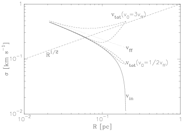
Figure 1: Left panel: The solid line shows the trajectory in the ${\cal L}$ vs. $\Sigma$ plane of a core of fixed mass $M=1$ $M_{\odot}$ that becomes Jeans-unstable, beginning to collapse at a time $t_{0}$, at which it has an initial radius $R_{0}=0.2$ pc, implying an initial column density $\Sigma_{0}$, shown by the vertical dashed-dotted line. The dotted line shows the locus of a core of the same mass that contracts having always the free-fall speed, as given by eq. (6). The dashed lines show the evolutionary paths of 4 cores with a combined turbulent+gravitational velocity, as described by eq. (8). The upper (resp. lower) pair of dashed lines correspond to $v_{0}=3\sigma_{\rm ff}$ (resp. $v_{0}=1/2\sigma_{\rm ff}$). Of each of these pairs, the upper curve corresponds to $\eta=1/2$, appropriate for a Burgers spectrum, and the lower one to $\eta=2$, loosely representing dissipation in dense objects. Right panel The evolution of the same set of cores (with the same labeling of the lines) in the Larson diagram, $\sigma_{{\rm v,3D}}$ vs. $R$, represented by the dashed-dotted line.

Equation (5) implies that, as a non-turbulent core becomes unstable and begins to collapse, it follows the trajectory described by the solid line in the ${\cal L}$-vs.-$\Sigma$ diagram shown in the left panel of Fig. 1. This can be compared to the locus of a core of the same mass and initial radius, but assuming it has the free-fall velocity at all times, given by the dotted line in this figure. This implies that cores that start at rest and have not yet attained the full free-fall speed will in general appear sub-virial by an amount that depends on the time elapsed since collapse started. Finally, note that, in reality, the actual infall speed must be even lower because, as already pointed out by Larson (1969), at the early stages of collapse of an object of mass only slightly larger than the Jeans mass, the thermal pressure is not negligible, making the collapse slower than free fall.

2.2.2 Core with turbulence

Let us now consider that the full 3D velocity dispersion in the core, $\sigma_{\rm tot}$, contains an infall component, given by eq. (4) and a turbulent component $\sigma_{\rm turb}$, as discussed in Sec. 2.2 which may possibly depend on scale as

$$\sigma_{\rm turb}=v_{0}\left(\frac{R}{R_{0}}\right)^{\eta}.$$ (7)

Adding the infall and turbulent components of the velocity dispersion in quadrature, for such a core the corresponding Larson ratio is

$${\cal L}_{\rm tot}=\frac{\sigma_{\rm tot}}{R^{1/2}}=\left\{\frac{6\pi}{5}G\Sigma\left[1-\left(\frac{\Sigma_{0}}{\Sigma}\right)^{1/2}\right]+\frac{\sigma_{\rm turb}^{2}}{R}\right\}^{1/2},$$ (8)

The left panel of Fig. 1 also shows, with dashed lines, the evolutionary path of four cores following eq (8): two with initial turbulent dispersions $\sigma_{0}=\sigma_{\rm in}/2$ (dashed lines) and two with $\sigma_{0}=3\sigma_{\rm in}$ (dotted lines). In each pair, the upper curve corresponds to a scaling of $\sigma_{\rm turb}$ with $\eta=1/2$, which corresponds to supersonic turbulent saling (e.g., Burgers, 1948; Passot et al., 1988) while the lower one corresponds to $\eta=2$. This later value does not corresponds to a particular fluid regime, but allows us to represente the possibility that the turbulent component dissipates as the core is contracting.

The right panel of Fig. 1 shows the evolution of all these cases in the Larson diagram, $\sigma_{{\rm v,3D}}$$-R$, with the same line coding. It can be seen that, in general, the cores move transversely to the Larson linewidth-size relation, represented by the dotted curve, terminating their evolution in the upper-left part of the diagram, as first discussed by Ballesteros-Paredes et al. (2011a), and as do the cores in our numerical simulations (cf. Sec. 3.2 below).

A few points are worth noting about these curves. First, it can be seen that the contribution of the turbulent component to the velocity dispersion is most important at low column densities, for which the self-gravity-driven (i.e., infall) component is minimum. At higher column densities, the infall component becomes increasingly dominant. This is consistent with the result that the Larson ratio generally exhibits excesses over the equipartition value, or, equivalently, the virial parameter,

$$\alpha\equiv\frac{5{\sigma_{v,{\rm 3D}}}^{2}R}{GM},$$ (9)

is larger than unity, for low column density objects, both in observational (e.g., Barnes et al., 2011; Leroy et al., 2015) and numerical (Camacho et al., 2016) clump surveys.

Second, we stress that the turbulent component by no means needs to be interpreted as a supporting mechanism. As found by Camacho et al. (2016), this component corresponds, in roughly half of the low column density clouds or clumps, to large scale, external compressions that are assembling these objects, rather than supporting them.

Third, the transition from a domination of turbulent to the gravitational motions is due to the fact that the two follow different scalings: while in principle the turbulent velocity dispersion depends only on scale (eq. 7), regardless of column density (e.g., Padoan et al., 2016), the self-gravity-driven ones depend both on scale and column density (or mass), according to relation (1) (Heyer et al., 2009; Ballesteros-Paredes et al., 2011a; Camacho et al., 2016; Ibáñez-Mejía et al., 2016).

Fourth, note that clumps or cores that start with a low turbulent content may, during the initial stages of the contraction, exhibit a deficiency of the Larson ratio in relation to the equipartition (virial or free-fall) value. This may explain observations that find sub-virial cores (e.g., Kauffmann et al., 2013; Ohashi et al., 2016; Sanhueza et al., 2017).

Finally, it must be remembered that in the idealized study presented here, we have considered the monolithic collapse of a single clump over two orders of magnitude in column density, from values typical of large GMCs ($\sim 10$ $M_{\odot}$ pc^-2) to those of dense cores ($\sim 10^{3}$ $M_{\odot}$ pc^-2). In reality, such a range in column density is not accomplished by the collapse of a single object, but rather, through several stages of fragmentation. Thus, our result should only be taken as a first-order approximation to the effect of transitioning from an external, turbulence-dominated regime to an infall-dominated one.

3 Data

Since we want to understand the relative importance of turbulence and/or gravity in the process of star formation, we use both observational and numerical data of massive dense cores to study the kinematics of the gas before it forms stars. To accomplish this, we need to avoid the effects of stellar feedback in both datasets. In the case of the observational data, even though our cores are located in massive star-forming regions, we choose without morphological evidence of perturbations (e.g., jets or free-free emission due to ultra-compact HII regions). Also, we use ammonia, which might be destroyed in case of UV stellar feedback (e.g., Palau et al., 2014), which is expected to trace preferencially dense regions, rather than molecular flows, and requires large column densities to be detected. On the numerical side, stars are represented by sink particles that are allowed to acrette gas from their surrounding, but no feedback is prescribed in order to preserve the purely gravitational nature of the velocity field.

3.1 Observational data

We use recently published data of cores traced with NH₃ and/or CH₃CN, in order to map cores with high surface densities ($N\geq 10^{21}$cm^-2). Our sample of clumps and cores is taken from the works of Sepúlveda et al. (2011); Sánchez-Monge et al. (2013), and Hernández-Hernández et al. (2014). The first two works determine the properties from NH₃(1,1) and (2,2). The third sample includes cores studied in CH₃CN. The clumps and cores of the three samples include typical star-forming regions distributed all over the Galaxy, and are not focused on one single cloud, thus avoiding possible biases due to uncertainties in the distance determination, or to peculiarities of a given molecular cloud.

Finally, special care was taken in determining the linewidths, sizes and surface densities using the same method for all the samples. In particular, NH₃(1,1) linewidths were measured using the same routine in the GILDAS program CLASS, which takes into account the hyperfine structure of the NH₃(1,1) transition. The NH₃ abundance was adopted to be $4\times 10^{-8}$, as an average value of previous works (Pillai et al., 2006; Foster et al., 2009; Friesen et al., 2009; Rygl et al., 2010; Chira et al., 2013).

3.2 Numerical Simulations

In order to numerically investigate the evolution of cores in the $\sigma_{{\rm v,3D}}$$-R$ (“Larson”) and ${\cal L}$–$\Sigma$ diagrams, we performed 5 isothermal numerical simulations with Gadget-2, a Smoothed Particle Hydrodynamics (SPH) public code (Springel, 2005) to represent the interior of a small ($\sim$ parsec size) molecular cloud. We also include sink particles in the code, as in Jappsen et al. (2005).

Details of the simulations can be found in Ballesteros-Paredes et al. (2015). Here we just mention that these simulations were performed using 6 million particles, with a total mass of 1000 $M_{\odot}$ in a cubic open box of side 1 pc in all simulations but one. Three of the simulations had an initially homogeneous density field. We imposed initial velocity fluctuations using a purely rotational velocity power spectrum with random phases and amplitudes, as in Stone et al. (1998), and with a peak at wavenumber $k_{\rm for}=4\pi/L_{0}$,where $L_{0}$ is the linear size of the box. No forcing at later times is imposed. The initial Mach numbers of these runs were 16, 8 and 4, respectively, so we label them Runs M16, M8 and M4, respectively.

Additionally, we performed two other runs, for which the initial velocity field is zero. The first one, labeled Run M0-$\rho$K, has initial density fluctuations with a Kolmogorov-like power spectrum proportional to $k^{-5/3}$.

Finally, in the run labeled M0-$\rho$P, the initial density field is a Plummer sphere with $R_{c}=1$ pc, a size of 5 pc and a total mass of 4500$M_{\odot}$, again, with zero velocity field. Since the boxes are all strongly super-Jeans, all of them collapse within roughly one free-fall time. Furthermore, runs with non-zero velocity field exhibit a slight initial expansion, since we do not include any confining external medium.

The global evolution of all these runs can be generically described as follows: if the initial velocity field is not set to zero, the velocity fluctuations produce density enhancements while the turbulence is dissipated. The external parts of the cloud expand because there is no confining medium, but since the beginning, the bulk of the clouds’ mass starts to contract. This contraction, however, is noticeable only after some time, depending on the initial Mach number of the simulation: for run M16, it takes about 1/2 free-fall time $\tau_{\rm ff}$ for the collapse to begin, $\sim 1/4{\tau_{\rm ff}}$ for Mach 8 and only a small fraction of $\tau_{\rm ff}$ for the Mach 4 run. Once the initial imposed turbulence is dissipated, all runs proceed to collapse, lowering their sizes and increasing the velocity dispersion (although in this case, this nonthermal velocity dispersion is driven by self-gravity and corresponds to chaotic infall rather than actual turbulence that can provide support). Runs with no initial velocity field (runs M0-$\rho$K and M0-$\rho$P), only undergo this second part of the evolution, with the initial density fluctuations driving the local centers of collapse (see, e.g., Klessen & Burkert, 2000).

In order to understand the evolution of these clouds in the observational diagrams (Larson ratio vs. column density and velocity dispersion vs. size), we have defined 3 regions (“cores”) in the simulations for which we computed their mass, size and velocity dispersion at every time. These are spheres located at the center of the computational box, towards which the cloud is collapsing in a chaotic way due to the turbulent initial velocity fluctuations, and their sizes are defined so that they contain, at every time, 10, 25 and 50% of the mass of the whole cloud

The mass and the velocity dispersions are calculated straightforwardly, the former by just adding the mass of all the SPH particles sphere and the latter as the standard deviation of the particles’ velocities.

Finally, the clouds’ sizes are calculated as the Lagrangian size, i.e., as the cubic root of the sum of the volumes of all the SPH particles:

$$R=V_{\rm tot}^{1/3}=\left[m_{\rm sph}\sum_{i}{1\over\rho_{i}}\right]^{1/3}$$ (10)

where $\rho_{i}$ is the density of the $i^{\rm th}$ particle.

4 Results

4.1 Non-existence of a $\sigma_{{\rm v,3D}}$$-R$ relation

As mentioned in §1, Ballesteros-Paredes et al. (2011a) showed that current observational datasets using high-mass MC core observations in different kinds of regions do not exhibit the Larson (1981) $\sigma_{{\rm v,3D}}$$-R$ relation. Instead, they occupy the upper-left corner of the plane. Although such cores can be expected to have large column densities because they belong to massive star-forming regions, most of the data in the compilations discussed by Ballesteros-Paredes et al. (2011a) did not have estimations of the actual masses of the cores. Thus, the proposal that cores with larger column densities have larger velocity dispersions and smaller sizes still requires further testing using observational data that provide column density determinations that are independent of the velocity dispersion measurements.

In Figure 2a we plot our observational data sample in the Larson plane $\sigma_{{\rm v,3D}}$$-R$. W¡e use $\sigma_{{\rm v,3D}}$, defined as $\sqrt{3}~{}\sigma_{\rm v,obs}$, assuming that the three-dimensional velocity dispersion $\sigma_{{\rm v,3D}}$ is intrinsically isotropic, while the observed velocity dispersion $\sigma_{\rm v,obs}$ is only the projection of the former along the line of sight. The dataset is colored according to the column density of each core: purple diamonds represent the lowest column density points, ranging between 10 and 10²$M_{\odot}$pc^-2; light blue triangles represent the column density range 10²-10³ $M_{\odot}$pc^-2; red triangles, 10³-10⁴$M_{\odot}$pc^-2, and blue squares, 10⁴-10⁶$M_{\odot}$pc^-2. In addition, we highlight some cores with a dark circle, indicating those cores that are catalogued as quiescent and starless by Sánchez-Monge et al. (2013).

In this plot, the black dotted line represents the fit obtaned by Larson (1981), with a slope of 0.38, while the colored dashed lines represent lines of constant column density, assuming equipartition ($E_{\rm k}=|E_{\rm g,sph}|$) and that the cloud is spherical and has uniform density, so that

$$E_{\rm g,sph}=-{3\over 5}{GM^{2}\over R}.$$ (11)

Although there is substantial scatter due to the observational uncertainties, the cores follow a clear trend: higher-column density clumps have larger velocity dispersions and smaller sizes.

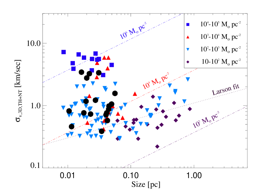
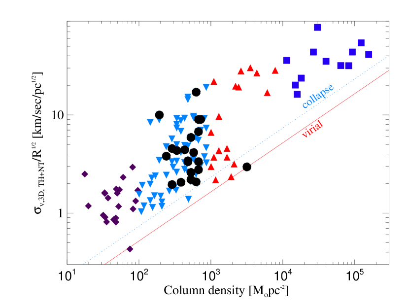
Figure 2: Right: Velocity dispersion vs. size for the compiled observational sample. Colors and symbols denote different ranges in column density, according to the labels. Lines of constant column density if non-thermal motions are driven by self-gravity are shown as dot-dashed lines. The original fit provided by Larson (1981) is shown with the solid line. In addition, we overlap with a dark solid circle those cores that have been catalogued as quiescent and starless. Left: same sample, in the Larson ratio ${\cal L}$ vs. column density $\Sigma$ space.

In Figure 2b we plot the ratio ${\cal L}\equiv$ $\sigma_{v,{\rm 3D}}/R^{1/2}$ against the column density $\Sigma$ for the same sample shown in Fig. 2a. Note that, if the clouds actually followed the two Larson relations (${\sigma_{v,{\rm 3D}}}\propto R^{1/2}$ and $n\propto R^{-1}$) simultanesouly, all data points would collapse to a single point in this plot (within the intrinsic scatter), as pointed out by Heyer et al. (2009). The red solid line in Fig. 2b represents the velocity dispersion of clouds in virial equilibrium, while the dashed line represents clouds in monolithic free-fall (cf. §2.2). We notice that, with some scatter, cores tend to follow a relation ${\sigma_{v,{\rm 3D}}}/R^{1/2}\propto\Sigma^{1/2}$, although for our sample, the cores have sistematically larger-than-virial values of the Larson ratio. Note that the clouds analyzed by Heyer et al. (2009) also exhibit larger-than-virial values, although those authors argued that this may have been due to their clouds’ masses possibly having been underestimated by factors $\sim 2$.

The fact that our data points are in general located above the virial-equilibrium and free-fall lines in the ${\cal L}$–$\Sigma$ plane would normally be interpreted as implying that the objects are not bound. However, this argument is somehow contradictory, since both our sample and the data of Heyer et al. (2009) contain high-column density objects, and thus they are likely to be strongly gravitationally bound. Moreover, note that, as evident in Fig. 2b, the free-fall line lies slightly above the virial equilibrium one; that is, the kinetic energy associated with free-fall is slightly larger than that associated with virial equilibrium. We will explore this point in §6.

4.2 Evolutionary trends of collapsing cores

In order to interpret the observational data, in particular the apparent average kinetic energy excess over equipartition of the whole sample, which is not predicted by the analytical model of Sec. 2.2, we now turn to the evolution of the cores in the numerical simulations.

In Fig. 3, we show the evolution of the cores in the Larson plane. As in Fig. 2b, the dotted line represents Larson’s original relation, with a slope of 0.38, while the dot-dashed lines represent lines of constant column density. For reference, the yellow area denotes the region occupied by the cores shown in Fig. 2a. In each panel, the evolution of the numerical cores is indicated with dashed lines, with red, dark purple and cyan representing the cores containing 10, 20 and 50% of the total mass in the box, respectively. The solid lines are discussed in the next section. The length of these trajectories corresponds to one free-fall time at the initial mean density for runs M16, M8 and M4, and to 0.8 free-fall times for the zero-velocity runs (M0-$\rho$K and M0-$\rho$P), since these simulations contain very dense regions where the timestep becomes too small, slowing the simulation down towards the end of the evolution. The triangles at the end of these lines indicate the place in which each core terminates its evolution. In all simulations, the cores with the higher masses have larger radii, so that the rightmost curves represent the evolution of the core with 50% of the mass, while the leftmost ones correspond to those with only 10% of the mass.

The evolution of the cores in the Larson diagram can be described as follows: Runs M16 and M8 initially exhibit a decrease in the velocity dispersion. The former does so at nearly constant size, while the latter does so while slightly lowering its size. This decrease corresponds to the initial period during which the excess turbulent energy dissipates. But, as gravity takes over, the sizes start decreasing more rapidly and the velocity dispersion starts increasing again, causing the cores to move towards the upper left in the Larson diagram. In the case of runs with small (M4) or no (M0-$\rho$K and M0-$\rho$P) initial turbulence, the cores only undergo the second stage, lowering their size while increasing their velocity dispersion.

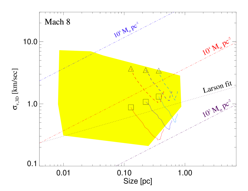
Figure 3: Dashed lines: evolution of the cores in the simulations in the Larson plane. Panels are organized as follows: (a) Run with initial Mach number 16. (b) Mach 8, (c) Mach 4, (d) Mach 0 with Kolmogorov density fluctuations, and (e) Mach 0, Plummer profile. Each curve represents aregion that contains 50% (rightmost curve), 25% and 10% (leftmost curve) of the mass at each time. Dashed lines are lines where energy equipartition is achieved at different column densities (see eq. (6). Solid lines: evolution of the cores in the simulations, but considering the correction factor defined in §5. Triangles and squares denote the last time in the evolution

In Fig. 4 we show the Larson ratio ${\cal L}=$ $\sigma_{v,{\rm 3D}}/R^{1/2}$ vs. the mass column density $\Sigma$ of the cores in our simulations. The lower and upper red dotted lines with slope 1/2 represent the locus of sphere with uniform density in virial equilibrium and in energy equipartition at the indicated column density, respectively. The yellow shaded area again denotes the region occupied by our observational data (see Fig. 2a).

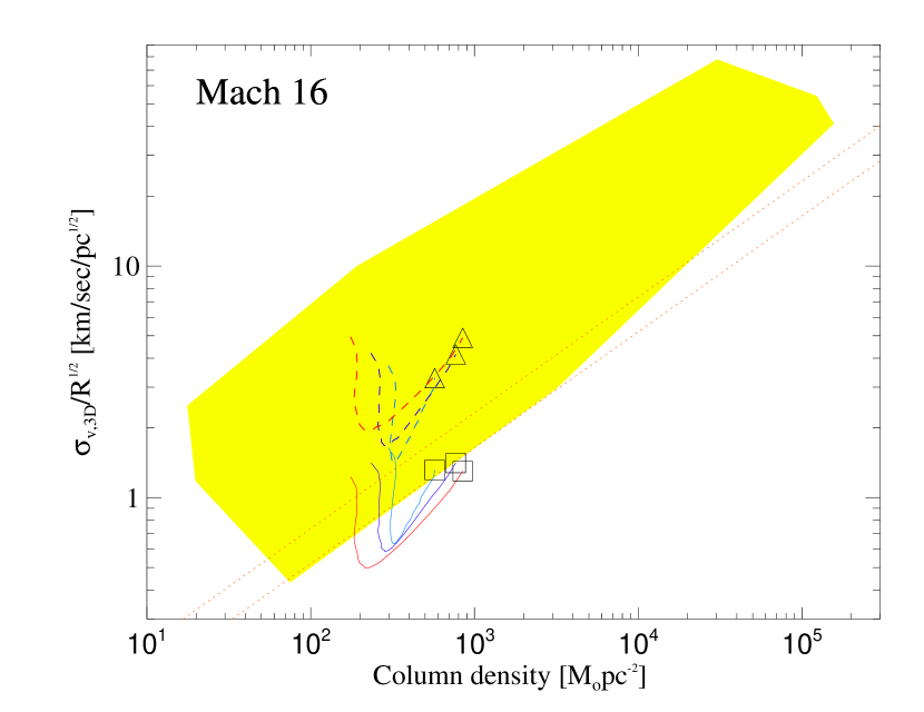
Figure 4: Dashed lines: evolution of the cores in the simulations in the Larson ratio-vs.-column density plane. Panels and notation, as in Fig. 3. The two lines in this figure denote the locus of the Virial and energy equipartition of a sphere with constant density.

The evolution of our cores in the Larson ratio-column density $\Sigma$ diagram is represented, again, by the dashed lines: red, dark purple and cyan representing the cores containing 10, 20 and 50% of the total mass in the box, respectively. As in the previous figure, the solid lines are discussed in the next section. As can be expected, runs with an excess of initial kinetic energy (M16, M8) lower their ${\cal L}$ ratio during the initial dissipation period, but as soon as gravity takes over, they increase it again, while their column density also increases. Instead, runs with low initial turbulence (M4) or without it (M0-$\rho$K and M0-$\rho$P) increase their Larson ratio ${\cal L}$ while they also increase their column density, in agreement with the prediction of the analytical model.

What seems to be surprising in Fig. 4 is that, even though the cores we show are all collapsing, they terminate their evolution exhibiting Larson ratios in excess of the equipartition and virial values corresponding to their column density. Thus, although our cores are not confined by any external medium and are collapsing, if only the information of this plot were provided, they would be naively interpreted either as expanding cores, or as cores that require an external confining pressure in order to be in virial equilibrium and to avoid their expansion.

Another point to notice is that the final column densities of the cores that would be inferred from their final position in the Larson diagram (comparing with the constant-column density lines in Fig. 3) are larger than their actual final column densities (as denoted by the abscissa of the triangles in Fig. 4). For instance, the Larson diagram would imply a column density of the order of $\sim$10⁴ $M_{\odot}$pc^-2 for the cores from run M16 (upper-left panel in Fig. 3), although they actually end their evolution with a column density of $\Sigma\sim 10^{3}$$M_{\odot}$pc^-2 (see the upper-left panel in Fig. 4). In the following section we will show that these results can be easily explained when the true gravitational energy of the cores, i.e., the gravitational energies considering the complex internal density structure.

5 Apparently supervirial collapsing cores: need for a correction factor

It is clear from the previous section that observed cores do not follow Larson’s velocity dispersion-size scaling relation, and may exhibit apparent excesses of kinetic energy when compared to the gravitational energy of a spherical cloud with constant density of the same mass and size, as is implicitly done by the standard virial equilibrium and equipartition lines drawn in Figs. 2b and 4.

In the standard picture, clouds/cores with such excesses are interpreted either as expanding (e.g., Dobbs et al., 2011), or as confined by an external medium (e.g., Keto & Myers, 1986; Bertoldi & McKee, 1992; Field et al., 2011). A frequent explanation of the origin of this apparent kinetic energy excess in those cores is that they belong to massive star forming regions, and thus they may be subject to kinetic energy injection from stellar feedback. However, at least in the case of the cores in our observational sample, the observed molecules (NH₃ and CH₃CN) are thought to not be seriously affected by stellar feedback: ammonia is destroyed by radiation and winds from stars, while CH₃CN requires large column densities to be detected, and thus it is unlikely that it comes from the outflows. In addition, even those cores that are known to be starless and quiescent in our sample (denoted by overlaid filled circles in Fig. 2b) also exhibit an excess of kinetic energy. In this case, how should we interpret this apparent excess?

To answer this question we turn to the simulations, in which the cores are collapsing and nevertheless still exhibit kinetic energies in excess of the corresponding gravitational energy as given by eq. (11). The solution to this apparent contradiction is actually rather simple: $E_{\rm g,sph}$, the gravitational energy of a sphere with constant density as given by eq. (11), is only a lower-limit to the magnitude of the actual gravitational content of the cloud. In practice, centrally concentrated density structures generally have a more negative gravitational energy than that of uniform-density structures of the same mass and size (see, e.g., Bertoldi & McKee, 1992); that is,

$$|E_{\rm g,real}|>|E_{\rm g,sph}|,$$ (12)

where $E_{\rm g,sph}$ is the approximation defined in eq. (11), and

$$E_{\rm g,real}=-{1\over 2}\int_{V}\rho\phi dV$$ (13)

is the true gravitational energy, in which

$$\phi=G\int_{\rm all\ space}{\rho(x^{\prime})\over|{\bf x}-{\bf x^{\prime}}|}dV$$ (14)

is the total gravitational potential, i.e., the potential produced by the mass distribution over all space, and not only inside the volume $V$ over which the integral in eq. (13) is performed. Therefore, by using the actual gravitational potential instead of eq. (11) for comparison with the kinetic energy, we can avoid the two approximations: the assumption of a constant density, and the neglect of the mass external to the cores. However, because both the Larson diagram and the ${\cal L}$–$\Sigma$ diagram involve the velocity dispersion, it is more convenient to introduce a correction factor to the velocity dispersion, which can be used in both diagrams.

Since at their late stages of evolution our cores are collapsing, either because the turbulent energy has been dissipated, or was not included at all, the non-thermal motions have a purely gravitational origin, and thus equipartition between kinetic and gravitational energy should hold at sufficiently late times during the evolution (cf. Sec. 2.2). Thus we write

$$E_{\rm k}=-E_{\rm g,real}.$$ (15)

Defining the factor

$$\Gamma\equiv{E_{\rm g,sph}\over W_{\rm cl}},$$

and subtituting it in eq. (15), we can compare the modified kinetic energy of each core with the gravitational energy of a sphere with constant density of the same mass and “size” $R$ (cf. eq. [10]) as the actual cloud. We obtain

$$\Gamma E_{\rm k}=-E_{\rm g,sph}.$$ (16)

From this equation it is clear that we need to multiply the measured ordinate axes of Figs. 3 and 4 by the factor $\Gamma$ in order to appropriately compare the kinetic energy of the cores to the gravitational energy of a homogeneous sphere, and so we define:

$$\left({\sigma_{v,{\rm 3D}}}\right)_{\rm corr} \equiv \Gamma\ {\sigma_{v,{\rm 3D}}}$$ (17)

$${\cal L}_{\rm corr} \equiv \Gamma{\cal L},$$ (18)

with ${\cal L}$ as defined by eq. (2). In Figs. 3 and 4 we thus respectively show, with solid lines, the velocity dispersion vs. size and the Larson ratio vs. column density diagrams with the corrected $y$ axes, as given by eqs. (17) and (18). In both cases, as expected, the values of the ordinates are now smaller than in the uncorrected case (dashed lines). But more importantly, now the values are consistent: the collapsing cores do not show an excess of kineitc energy compared to the gravitational content, and instead they terminate their evolution near the equipartition/virial lines in Fig. 4. Also, the final column densities predicted by the equipartition lines at constant column density in Fig. 3 (dot-dashed lines) are now in better agreement with the final column densities shown in Fig. 4. These results reflect the fact that collapse does induce virial-like equipartition (Vázquez-Semadeni et al., 2007; Ballesteros-Paredes et al., 2011a).

Finally, we also note that the location of our cores in the diagrams depends on their evolutionary stage, as discussed in §2.2. Although we have not run the simulations more than one free-fall time because the timestep of the simulation becomes too short as collapse proceeds, the evolutionary tracks, as well as the simple model discussed in §2.2, suggest that further evolution in the Larson’s ratio-column density diagram is expected to proceed roughly along the virial/equipartition lines. If a similar correction is applicable to the observational sample, then its locus in the Larson ratio-column density diagram would be in closer agreement with equipartition/virial balance, suggesting that the internal motions of the cores in the sample are indeed dominated by gravity. Furthermore, the evolution in the Larson diagram should be expected to be oblique to the lines of constant column density, with a slope that should approach $-1/2$, since

$$\sigma\propto\sqrt{\Sigma R}\propto{R^{-1/2}}$$ (19)

at constant mass, as is the case of the cores discussed in this section and in Sec. 2.2.

6 Discussion

Traditionally, the apperent near-virialization exhibited by clouds and their substructures (clumps and dense cores) has been interpreted as a manifestation that all the structures in this hierarchy are supported against their self-gravity by strongly supersonic turbulence, and that, when this turbulence dissipates at the smallest scales, the cores can then proceed to collapse (see, e.g., the reviews by Larson, 1981; Vázquez-Semadeni et al., 2000; Mac Low & Klessen, 2004; Ballesteros-Paredes et al., 2007; McKee & Ostriker, 2007; Bergin & Tafalla, 2007; Hennebelle & Falgarone, 2012; Dobbs et al., 2014; Donkov et al., 2011, 2012; Veltchev et al., 2016). However, it is difficult to understand how the many energy-injection mechanisms could adjust themselves to provide just the right amount of energy to the turbulence to keep the structures nearly virialized at all scales. Some authors have proposed, on the basis of idealized models for the star formation rate (e.g., Krumholz et al., 2006; Goldbaum et al., 2011), that the feedback from stellar sources internal to the clouds can self-regulate to attain near virialization. However, evolutionary models (Zamora-Avilés et al., 2012; Zamora-Avilés & Vázquez-Semadeni, 2014), as well as numerical simulations (e.g., Vázquez-Semadeni et al., 2010; Dale et al., 2012, 2013a, 2013b; Colín et al., 2013) do not show a trend towards local virialization, but rather, towards local destruction of the star-forming sites.

On the other hand, it is also sometimes suggested that feedback from sources external to the clouds can drive the turbulence at all scales within the clouds (e.g., Padoan et al., 2016). The underlying assumption here is that this is a natural consequence of the turbulent cascade, as the energy spectrum of Burgers-like strongly supersonic turbulence should approach the form $E(k)\propto k^{-2}$, where $k$ is the wavenumber. This spectrum implies a velocity dispersion-size scaling relation of the form $\sigma\propto R^{1/2}$, similar to Larson’s scaling, and thus strongly supersonic turbulence has been proposed as the origin of the Larson scaling. However, as shown in several observational and numerical studies (Heyer et al., 2009; Ballesteros-Paredes et al., 2011a; Leroy et al., 2015; Camacho et al., 2016, this work; although see Padoan et al. 2016), the Larson scaling is not universal, and instead the Larson ratio ${\cal L}$, which should be constant for strongly supersonic turbulence, is actually dependent on the column density as $\Sigma^{1/2}$, suggesting that the process does not rely only on the turbulent cascade.

More specifically, within the scatter, cores tend to be organized by column density along lines with slope 1/2 in the Larson ${\sigma_{v,{\rm 3D}}}$-$R$ diagram, with high-column density cores being located on the upper-left part of the diagram, and low-column density cores appearing at lower velocity dispersions at a given value of $R$. Moreover, regardless of the observational uncertanties, not all cores with the same column density will necessarily be located exactly at the same position in the ${\cal L}$–$\Sigma$ diagram, since their exact position on the diagrams depends on their evolutionary stage, as the results from §§2.2 and 4.2 show.

The observational sample considered here also shows a correlation between the Larson ratio ${\cal L}$ and the column density in general agreement with eq. (1), although on average it exhibits somewhat supervirial values when the gravitational energy of the sample cores is computed using eq. (11) (e.g., Heyer et al., 2009; Leroy et al., 2015), which assumes that the cloud is a uniform-density sphere. Although we cannot discard stellar feedback in the observations, the facts that a) our sample was observed with tracers that should not be strongly affected by feedback; b) the subsample of quiescent starless cores exhibits the same behavior, and c) simulations of collapsing cores also exhibit overvirialization, lead us to conclude that such apparent overvirialization may be spurious. Indeed, we find that, when the kinetic energy is corrected by a factor equal to the ratio of the actual gravitational energy to that given by eq. (11), then the apparent excess of kinetic energy essentially disappears.

On the other hand, surveys of massive star-forming cores sometimes exhibit subvirial values of the Larson ratio, a result which has often been interpreted as the cores being supported by some form of energy other than the turbulent pressure, such as the magnetic pressure (e.g., Kauffmann et al., 2013; Ohashi et al., 2016; Sanhueza et al., 2017) , or else as the cores being already in full-blown collapse, i.e., at the full free-fall speed, rather than the lower infall speed given by eq. (4). However, because the infall speeds are also nonthermal motions, full-blown collapse should correspond to a virial ratio (cf. eq. [9]) $\alpha\sim 2$, not to $\alpha<1$. Although magnetic support for these cores is indeed a plausible explanation, we have shown that, when a core begins its own local collapse, it may start with subvirial velocities if its intial turbulent energy is sufficiently low, approaching the virial value from below. This constitutes an alternative plausible explanation for the observations of subvirial cores.

The notion that the nonthermal motions observed in MCs are produced by the collapse itself is contrary to the widespread notion that turbulence is the main physical process controlling the internal dynamics of MCs, providing support to MCs and causing their fragmentation. Although the turbulent density fluctuations in the diffuse medium may very well play a crucial role in the formation of the seeds of what eventually will grow as cores via instabilities, the fluctuations produced self-consistently by this mechanism are generally not strong enough to become locally Jeans unstable, until global collapse has significantly reduced the mean Jeans mass in the cloud (e.g., Koyama & Inutsuka, 2002; Heitsch et al., 2005; Clark & Bonnell, 2005; Vázquez-Semadeni et al., 2007; Heitsch & Hartmann, 2008). Moreover, observational data show that fragmentation levels within dense cores do not correlate with the intensity of the observed non-thermal motions (Palau et al., 2015), again suggesting that they actually do not consist of random turbulent fluctuations. Nevertheless, the fluctuations produced by the growth of seeds triggered by the global collapse do contain a significant fraction of chaotic motions due to the turbulent background, and so theese fluctuations are far from being ordered and monolithic. Indeed, Heitsch et al. (2009) showed that clouds in a state of hierarchical gravitational collapse do exhibit line profiles similar to observed MCs in the structure of the CO lines, the supersonic widths, and their core-to-core velocity dispersion. However, the net average component of the velocity field continues to be dominated by global contraction, as shown by studies of the dense regions in simulations of driven, isothermal turbulence, which indicate that the overdensities tend to have a negative net velocity divergence (i.e., a convergence) (e.g. Vázquez-Semadeni et al., 2008; González-Samaniego et al., 2014; Camacho et al., 2016). Thus, the density fluctuations are in general contracting, rather than being completely random with zero or positive net divergence, as would be necessary for the bulk motions to exert a “turbulent pressure” capable of opposing the self-gravity of the overdensities. If the non-thermal motions in the clumps and cores do not exert a turbulent pressure capable of providing support against the self-gravity of the structures, then MC models based on the competition between gravity and turbulent support may need to be revisited (e.g., McKee & Tan, 2003; Krumholz & McKee, 2005; Hennebelle & Chabrier, 2008, 2011; Hopkins, 2012).

7 Conclusions

In this paper we have used observational data and numerical simulations to show that the scaling relation between velocity dispersion and size does not hold when column densities spanning a large dynamic range are considered. In this case, cores with large column densities tend to be located in the upper-left corner of the Larson velocity dispersion-size diagram. Using numerical simulations, we showed that, as cores collapse, their sizes become smaller and their column densities larger, and thus, their evolution tends to follow lines oblique to the $\sigma_{{\rm v,3D}}$$\propto R^{1/2}$ relation.

Additionally, we showed analytically that, as cores evolve from when they first detach from the global flow and begin their local collapse, they may exhibit subvirial velocities if their internal turbulent component is initially low enough. This is because, when the core first starts to collapse locally, its gravitationally-driven speed starts out from zero, and takes a finite amount of time to reach the full free-fall speed. This behavior was observed also in the numerical simulations that start with little or no turbulent energy, and it may explain recent observations of apparently sub-virial cores (e.g., Kauffmann et al., 2013; Ohashi et al., 2016; Sanhueza et al., 2017).

We also showed that, although the observed cores were selected to avoid stellar feedback, they appear to be supervirial. However, this feature is likely due to the fact that, rather than comparing the kinetic energy to the actual gravitational content of the core, $W$, in practice it is customary to use the gravitational energy of a sphere with constant density as a proxy for $W$. This proxy actually provides only a lower limit (in absolute value) to the actual value of $W$. We show that, indeed, this is the case in our simulations: collapsing cores do exhibit over-virial velocities at the end of their evolution, and thus end up in the virial/equipartition zone. Thus, the virial parameter computed using the uniform sphere approximation should be taken with caution when interpreting their observational data.

This work then provides support to the scenario that non-thermal motions in MCs have largely a gravitational origin and are dominated by infall motions. Because of the rapid dissipation of turbulence, the conversion of the infall motions into random, truly turbulent motions that can oppose the collapse that produces them in the first place does not appear feasible. In a future contribution, we plan to further explore this possibility.

8 Acknowledgments

This work was supported by UNAM-PAPIIT grant number IN110816 to JBP and CONACYT grant 255295 to E.V.-S. In addition, J.B.P. acknowledges the hospitality of the Institute for Theoretical Astrophysics of the University of Heidelberg, as well as UNAM’s DGAPA-PASPA Sabbatical program. He also is indebted to the Alexander von Humboldt Stiftung for its valuable support. RSK acknowledges support from the Deutsche Forschungsgemeinschaft in the Collaborative Research Center SFB 881 “The Milky Way System” (subprojects B1, B2, and B8) and in the Priority Program SPP 1573 “Physics of the Interstellar Medium” (grant numbers KL 1358/18.1, KL 1358/19.2). RSK furthermore thanks the European Research Council for funding in the ERC Advanced Grant STARLIGHT (project number 339177). Numerical simulations were performed in the supercomputer Miztli, at DGTIC-UNAM. We have made extensive use of the NASA-ADS database.

References

- Audit & Hennebelle (2005) Audit, E., & Hennebelle, P. 2005, A& A, 433, 1
- Ballesteros-Paredes (2006) Ballesteros-Paredes, J. 2006, MNRAS, 372, 443
- Ballesteros-Paredes et al. (2012) Ballesteros-Paredes, J., D’Alessio, P., & Hartmann, L. 2012, MNRAS, 427, 2562
- Ballesteros-Paredes et al. (2015) Ballesteros-Paredes, J., Hartmann, L. W., Pérez-Goytia, N., & Kuznetsova, A. 2015, MNRAS, 452, 566
- Ballesteros-Paredes et al. (1999b) Ballesteros-Paredes, J., Hartmann, L., & Vázquez-Semadeni, E. 1999, ApJ, 527, 285
- Ballesteros-Paredes et al. (2011a) Ballesteros-Paredes, J., Hartmann, L. W., Vázquez-Semadeni, E., Heitsch, F., & Zamora-Avilés, M. A. 2011, MNRAS, 411, 65
- Ballesteros-Paredes et al. (2007) Ballesteros-Paredes, J., Klessen, R. S., Mac Low, M.-M., & Vazquez-Semadeni, E. 2007, Protostars and Planets V, 63
- Ballesteros-Paredes & Mac Low (2002) Ballesteros-Paredes, J., & Mac Low, M.-M. 2002, ApJ, 570, 734
- Ballesteros-Paredes et al. (2011b) Ballesteros-Paredes J., Vázquez-Semadeni E., Gazol A., Hartmann L. W., Heitsch F., Colín P., 2011, MNRAS, 416, 1436
- Ballesteros-Paredes et al. (1999a) Ballesteros-Paredes, J., Vázquez-Semadeni, E., & Scalo, J. 1999, ApJ, 515, 286
- Barnes et al. (2011) Barnes, P. J., Yonekura, Y., Fukui, Y., et al. 2011, ApJS, 196, 12
- Beaumont et al. (2012) Beaumont, C. N., Goodman, A. A., Alves, J. F., et al. 2012, MNRAS, 423, 2579
- Bergin & Tafalla (2007) Bergin, E. A., & Tafalla, M. 2007, ARA&A, 45, 339
- Bertoldi & McKee (1992) Bertoldi, F., & McKee, C. F. 1992, ApJ, 395, 140
- Brunt et al. (2009) Brunt, C. M., Heyer, M. H., & Mac Low, M.-M. 2009, A& A, 504, 883
- Burgers (1948) 1948, Adv. Appl. Mech., 1, 171
- Camacho et al. (2016) Camacho, V., et al., 2016, ApJ, in press
- Chira et al. (2013) Chira R.-A., Beuther H., Linz H., Schuller F., Walmsley C. M., Menten K. M., Bronfman L., 2013, A&A, 552, A40
- Clark & Bonnell (2005) Clark, P. C., & Bonnell, I. A. 2005, MNRAS, 361, 2
- Colín et al. (2013) Colín, P., Vázquez-Semadeni, E., & Gómez, G. C. 2013, MNRAS, 435, 1701
- Dale et al. (2012) Dale, J. E., Ercolano, B., & Bonnell, I. A. 2012, MNRAS, 424, 377
- Dale et al. (2013a) Dale, J. E., Ercolano, B., & Bonnell, I. A. 2013, MNRAS, 430, 234
- Dale et al. (2013b) Dale, J. E., Ngoumou, J., Ercolano, B., & Bonnell, I. A. 2013, MNRAS, 436, 3430
- Dobbs et al. (2011) Dobbs, C. L., Burkert, A., & Pringle, J. E. 2011, MNRAS, 413, 2935
- Dobbs et al. (2014) Dobbs, C. L., Krumholz, M. R., Ballesteros-Paredes, J., et al. 2013, arXiv:1312.3223
- Donkov et al. (2011) Donkov, S., Veltchev, T. V., & Klessen, R. S. 2011, MNRAS, 418, 916
- Donkov et al. (2012) Donkov, S., Veltchev, T. V., & Klessen, R. S. 2012, MNRAS, 423, 889
- Elmegreen & Scalo (2004) Elmegreen, B. G., & Scalo, J. 2004, ARA&A, 42, 211
- Falgarone et al. (1991) Falgarone, E., Phillips, T. G., & Walker, C. K. 1991, ApJ, 378, 186
- Federrath et al. (2008) Federrath, C., Klessen, R. S., & Schmidt, W. 2008, ApJL, 688, L79
- Field et al. (2011) Field, G. B., Blackman, E. G., & Keto, E. R. 2011, MNRAS, 416, 710
- Foster et al. (2009) Foster J. B., Rosolowsky E. W., Kauffmann J., Pineda J. E., Borkin M. A., Caselli P., Myers P. C., Goodman A. A., 2009, ApJ, 696, 298
- Friesen et al. (2009) Friesen R. K., Di Francesco J., Shirley Y. L., Myers P. C., 2009, ApJ, 697, 1457
- Gatto et al. (2015) Gatto, A., Walch, S., Low, M.-M. M., et al. 2015, MNRAS, 449, 1057
- Goldbaum et al. (2011) Goldbaum, N. J., Krumholz, M. R., Matzner, C. D., & McKee, C. F. 2011, ApJ, 738, 101
- Goldreich & Kwan (1974) Goldreich, P., & Kwan, J. 1974, ApJ, 189, 441q
- Gómez & Vázquez-Semadeni (2014) Gomez, G. C., & Vazquez-Semadeni, E. 2014, ApJ, 791, 124
- González-Samaniego et al. (2014) González-Samaniego, A., Vázquez-Semadeni, E., González, R. F., & Kim, J. 2014, MNRAS, 440, 2357
- Hartmann et al. (2001) Hartmann, L., Ballesteros-Paredes, J., & Bergin, E. A. 2001, ApJ, 562, 852
- Hartmann et al. (2012) Hartmann, L., Ballesteros-Paredes, J., & Heitsch, F. 2012, MNRAS, 420, 1457
- Heitsch et al. (2009) Heitsch, F., Ballesteros-Paredes, J., & Hartmann, L. 2009, ApJ, 704, 1735
- Heitsch et al. (2005) Heitsch, F., Burkert, A., Hartmann, L. W., Slyz, A. D., & Devriendt, J. E. G. 2005, ApJL, 633, L113
- Heitsch & Hartmann (2008) Heitsch, F., & Hartmann, L. 2008, ApJ, 689, 290
- Hennebelle & Chabrier (2008) Hennebelle, P., & Chabrier, G. 2008, ApJ, 684, 395
- Hennebelle & Chabrier (2011) Hennebelle, P., & Chabrier, G. 2011, ApJL, 743, L29
- Hennebelle & Falgarone (2012) Hennebelle, P., & Falgarone, E. 2012, A& A Rev., 20, 55
- Hennebelle & Pérault (1999) Hennebelle, P., & Pérault, M. 1999, A& A, 351, 309
- Hernández-Hernández et al. (2014) Hernández-Hernández V., Zapata L., Kurtz S., Garay G., 2014, ApJ, 786, 38
- Heyer et al. (2009) Heyer, M., Krawczyk, C., Duval, J., & Jackson, J. M. 2009, ApJ, 699, 1092
- Hopkins (2012) Hopkins, P. F. 2012, MNRAS, 423, 2016
- Ibáñez-Mejía et al. (2016) Ibáñez-Mejía, J. C., Mac Low, M.-M., Klessen, R. S., & Baczynski, C. 2016, ApJ, 824, 41
- Jappsen et al. (2005) Jappsen, A.-K., Klessen, R. S., Larson, R. B., Li, Y., & Mac Low, M.-M. 2005, A& A, 435, 611
- Kainulainen et al. (2009) Kainulainen, J., Beuther, H., Henning, T., & Plume, R. 2009, A& A, 508, L35
- Kauffmann et al. (2013) Kauffmann, J., Pillai, T., & Goldsmith, P. F. 2013, ApJ, 779, 185
- Kauffmann et al. (2010) Kauffmann, J., Pillai, T., Shetty, R., Myers, P. C., & Goodman, A. A. 2010, ApJ, 712, 1137
- Kauffmann et al. (2010) Kauffmann, J., Pillai, T., Shetty, R., Myers, P. C., & Goodman, A. A. 2010, ApJ, 716, 433
- Keto & Myers (1986) Keto, E. R., & Myers, P. C. 1986, ApJ, 304, 466
- Klessen & Burkert (2000) Klessen, R. S., & Burkert, A. 2000, ApJS, 128, 287
- Klessen & Glover (2016) Klessen, R. S., & Glover, S. C. O. 2016, Star Formation in Galaxy Evolution: Connecting Numerical Models to Reality, Saas-Fee Advanced Course, Volume 43. ISBN 978-3-662-47889-9. Springer-Verlag Berlin Heidelberg, 2016, p. 85, 43, 85
- Klessen & Hennebelle (2010) Klessen, R. S., & Hennebelle, P. 2010, A& A, 520, A17
- Koyama & Inutsuka (2000) Koyama, H., & Inutsuka, S.-I. 2000, ApJ, 532, 980
- Koyama & Inutsuka (2002) Koyama, H., & Inutsuka, S.-i. 2002, ApJL, 564, L97
- Kritsuk et al. (2011) Kritsuk, A. G., Norman, M. L., & Wagner, R. 2011, ApJL, 727, L20
- Krumholz & McKee (2005) Krumholz, M. R., & McKee, C. F. 2005, ApJ, 630, 250
- Krumholz et al. (2006) Krumholz, M. R., Matzner, C. D., & McKee, C. F. 2006, ApJ, 653, 361
- Larson (1969) Larson, R. B. 1969, MNRAS, 145, 271
- Larson (1981) Larson, R. B. 1981, MNRAS, 194, 809
- Leroy et al. (2015) Leroy, A. K., Bolatto, A. D., Ostriker, E. C., et al. 2015, ApJ, 801, 25
- Liszt et al. (1974) Liszt, H. S., Wilson, R. W., Penzias, A. A., et al. 1974, ApJ, 190, 557
- Lombardi et al. (2010) Lombardi, M., Alves, J., & Lada, C. J. 2010, A& A, 519, L7
- Mac Low & Klessen (2004) Mac Low M.-M., Klessen R. S., 2004, RvMP, 76, 125
- McKee & Ostriker (2007) McKee, C. F., & Ostriker, E. C. 2007, ARA&A, 45, 565
- McKee & Tan (2003) McKee, C. F., & Tan, J. C. 2003, ApJ, 585, 850
- Miville-Deschênes et al. (2016) Miville-Deschênes, M.-A., Murray, N., & Lee, E. J. 2016, arXiv:1610.05918
- Norman & Ferrara (1996) Norman, C. A., & Ferrara, A. 1996, ApJ, 467, 280
- Ohashi et al. (2016) Ohashi, S., Sanhueza, P., Chen, H.-R. V., et al. 2016, ApJ, 833, 209
- Padoan et al. (2014) Padoan, P., Federrath, C., Chabrier, G., et al. 2014, Protostars and Planets VI, 77
- Padoan et al. (2016) Padoan, P., Pan, L., Haugbølle, T., & Nordlund, Å. 2016, ApJ, 822, 11
- Palau et al. (2015) Palau, A., Ballesteros-Paredes, J., Vázquez-Semadeni, E., et al. 2015, MNRAS, 453, 3785
- Palau et al. (2014) Palau, A., Estalella, R., Girart, J. M., et al. 2014, ApJ, 785, 42
- Passot et al. (1988) Passot, T., Pouquet, A., & Woodward, P. 1988, A& A, 197, 228
- Pillai et al. (2006) Pillai T., Wyrowski F., Carey S. J., Menten K. M., 2006, A&A, 450, 569
- Roman-Duval et al. (2010) Roman-Duval, J., Jackson, J. M., Heyer, M., Rathborne, J., & Simon, R. 2010, ApJ, 723, 492
- Rygl et al. (2010) Rygl K. L. J., Wyrowski F., Schuller F., Menten K. M., 2010, A&A, 515, A42
- Sánchez-Monge et al. (2013) Sánchez-Monge Á., et al., 2013, MNRAS, 432, 3288
- Sanhueza et al. (2017) Sanhueza, P., Jackson, J. M., Zhang, Q., et al. 2017, ApJ, 841, 97
- Sepúlveda et al. (2011) Sepúlveda I., Anglada G., Estalella R., López R., Girart J. M., Yang J., 2011, A&A, 527, A41
- Solomon et al. (1987) Solomon, P. M., Rivolo, A. R., Barrett, J., & Yahil, A. 1987, ApJ, 319, 730
- Springel (2005) Springel, V. 2005, MNRAS, 364, 1105
- Stone et al. (1998) Stone, J. M., Ostriker, E. C., & Gammie, C. F. 1998, ApJL, 508, L99
- Traficante et al. (2016) Traficante, A., Fuller, G. A., Smith, R., et al. 2016, EAS Publications Series, 75, 185
- Vázquez-Semadeni (2015) Vázquez-Semadeni, E. 2015, Magnetic Fields in Diffuse Media, 407, 401
- Vázquez-Semadeni et al. (2010) Vázquez-Semadeni, E., Colín, P., Gómez, G. C., Ballesteros-Paredes, J., & Watson, A. W. 2010, ApJ, 715, 1302
- Vázquez-Semadeni et al. (2007) Vázquez-Semadeni, E., Gómez, G. C., Jappsen, A. K., et al. 2007, ApJ, 657, 870
- Vázquez-Semadeni et al. (2009) Vázquez-Semadeni, E., Gómez, G. C., Jappsen, A.-K., Ballesteros-Paredes, J., & Klessen, R. S. 2009, ApJ, 707, 1023
- Vázquez-Semadeni et al. (2008) Vázquez-Semadeni, E., González, R. F., Ballesteros-Paredes, J., Gazol, A., & Kim, J. 2008, MNRAS, 390, 769
- Vázquez-Semadeni et al. (2017) Vázquez-Semadeni, E., González-Samaniego, A., & Colín, P. 2017, MNRAS, 467, 1313
- Vázquez-Semadeni et al. (2005) Vázquez-Semadeni, E., Kim, J., Shadmehri, M., & Ballesteros-Paredes, J. 2005, ApJ, 618, 344
- Vázquez-Semadeni et al. (2000) Vazquez-Semadeni, E., Ostriker, E. C., Passot, T., Gammie, C. F., & Stone, J. M. 2000, Protostars and Planets IV, 3
- Vazquez-Semadeni et al. (1996) Vazquez-Semadeni, E., Passot, T., & Pouquet, A. 1996, ApJ, 473, 881
- Vázquez-Semadeni et al. (2006) Vázquez-Semadeni, E., Ryu, D., Passot, T., González, R. F., & Gazol, A. 2006, ApJ, 643, 245
- Veltchev et al. (2016) Veltchev, T. V., Donkov, S., & Klessen, R. S. 2016, MNRAS, 459, 2432
- Vishniac (1994) Vishniac, E. T. 1994, ApJ, 428, 186
- Walder & Folini (2000) Walder, R., & Folini, D. 2000, Ap& SS, 274, 343
- Wang et al. (2010) Wang, P., Li, Z.-Y., Abel, T., & Nakamura, F. 2010, ApJ, 709, 27
- Zamora-Avilés et al. (2012) Zamora-Avilés, M., Vázquez-Semadeni, E., & Colín, P. 2012, ApJ, 751, 77
- Zamora-Avilés & Vázquez-Semadeni (2014) Zamora-Avilés, M., & Vázquez-Semadeni, E. 2014, ApJ, in press (arXiv:1308.4918)
- Zuckerman & Palmer (1974) Zuckerman, B., & Palmer, P. 1974, ARA&A, 12, 279