AdS/QCD duality and the quarkonia holographic information entropy

Abstract

Bottomonium and charmonium, representing quarkonia states, are scrutinized under the point of view of the information theory, in the AdS/QCD holographic setup. A logarithmic measure of information, comprised by the configurational entropy, is here employed to quantitatively study quarkonia radially excited $S$-wave states. The configurational entropy provides data regarding the relative dominance and the abundance of the bottomonium and charmonium states, whose underlying information is more compressed, in the Shannon’s theory meaning. The derived configurational entropy, therefore, identifies the lower phenomenological prevalence of higher $S$-wave resonances and higher masses quarkonia in Nature.

I Introduction

The configurational (CE) entropy is a paradigm, contemporarily proposed on the beginning of this decade Gleiser:2011di ; Gleiser:2012tu , that considers foreseeable aspects of information into general systems. The configurational entropy, as a logarithmic quantity of information, measures the form intricacy of localized, Lebesgue-integrable, physical configurations of general systems Gleiser:2014ipa ; Sowinski:2015cfa ; Gleiser:2012tu . The CE, which directly measures the compression of lossless data into the frequency modes of a system, is derived from the physical system configuration via a Fourier transform. It expresses the quantity of the organizational capacity enciphered into the energy density describing a physical system, as the temporal component of the energy-momentum tensor of the theory. Beyond the principle of least action, where physical systems extremize the corresponding action, the CE, in addition, points to either more stable states, or to more abundant/dominant ones. Physical states with higher CE either require more energy to be produced in Nature, or are less observed/detected than their CE-stable peer states, or even both. The lattice approach of Shannon information entropy has the information dimension, driving data distributions, as an upper bound for the compression data rate of any variable in a distribution. Statistical-mechanics grounds were introduced in this context, in the literature Bernardini:2016hvx . The CE encodes the precise measurement of information that is mandatory to account the spatial shape of Lebesgue-integrable functions, with respect to their parametrical arguments.

The CE has been used to derive the abundance of light-flavor mesons in AdS/QCD holographic models, both in the asymptotically AdS₅ metric of $D_{3}$ brane systems and in the Sakai–Sugimoto $D_{4}$-$D_{8}$ system, as well, in Ref. Bernardini:2016hvx . Besides, glueball phenomenology, their stability and the relative dominance of their states, according to their spin, were investigated in the context of the CE, in the AdS/QCD setup Bernardini:2016qit . The CE was also used in QCD models to study and refine cross-sections of hadrons in the color-glass condensate Karapetyan:2016fai ; Karapetyan:2017edu . Moreover, the CE was employed to study AdS-Schwarzschild black holes Braga:2016wzx ; Lee:2017ero , in a consistent setup that corroborates to the consistency of the Hawking-Page phase transition Braga:2016wzx , and also to study compact stars Gleiser:2013mga ; Gleiser:2015rwa , including the prediction of the Chandrasekhar critical density of a Bose–Einstein condensate of gravitons into compact stars, on fluid branes Casadio:2016aum . Solitons in a cold quark-gluon plasma were further investigated with the CE, in Ref. daSilva:2017jay , to derive the pulse soliton width for which the soliton spatial profile has more compressed information, matching phenomenological data. In addition, the CE was successfully utilized in particle physics to determine the Higgs boson mass Alves:2017ljt and to derive the precise mass of an axion that interacts with neutrinos and photons Alves:2014ksa . Other topological defects were also scrutinized in the context of the CE Correa:2015vka ; Correa:2016pgr .

The fundamental theory of strong interactions, quantum chromodynamics (QCD), presents a coupling constant that increases as the energy decreases. This is the reason why there are many important hadronic properties that can not be perturbatively described by QCD. An interesting complementary tool for studying hadronic states in the vacuum or at finite temperature and (or) density are the AdS/QCD models. This approach is motivated by the AdS/CFT correspondence Maldacena:1997re ; Gubser:1998bc ; Witten:1998qj , relating weakly coupled supergravity in five dimensional anti-de Sitter space (AdS₅) to a conformal super Yang-Mills theory on the boundary. Phenomenological AdS/QCD models assume the existence of a similar type of duality in cases where conformal invariance is broken by the introduction of an energy parameter in the AdS background, representing an infrared (IR) cut-off – mass scale – in the gauge theory. The simplest one is the hard wall model, proposed in Refs. Polchinski:2001tt ; BoschiFilho:2002ta ; BoschiFilho:2002vd , that consists in placing a hard cut-off in anti-de Sitter (AdS) space. Another AdS/QCD model is the soft wall one, that has the property that the square of the mass linearly grows with the radial excitation number Karch:2006pv . In this case, the background involves an AdS space and a scalar field that effectively acts as a smooth infrared cut-off. A review of AdS/QCD models can be found in Ref. Brodsky:2014yha .

Quarkonia are hadronic states made of a heavy quark-antiquark pair. For the vectorial case, they are the charmonium $J/\psi$ meson, composed by a charmed $\bar{c}c$ pair, the bottomonium $\Upsilon$ meson, made of a $\bar{b}b$ pair, and their corresponding radial excitations. Due to the high mass of the top quark, toponium does not exist. In fact, the top quark decays through the electroweak interaction before a bound state can form, providing a rare example of a weak process proceeding more quickly than a strong process. Usually in the literature, the word quarkonium refers only to charmonium and bottomonium, and not to any of the lighter quark-antiquark states Bernardini:2003ht .

A consistent AdS/QCD model for charmonium and bottomonium in the vacuum was recently proposed in Braga:2015jca , extended to finite temperature in Braga:2016wkm and to finite density and temperature in Braga:2017oqw . There are two different energy parameters in this model. One infrared mass scale and one large ultraviolet scale, related to the non hadronic decay of the heavy vector mesons. The model of Ref. Braga:2015jca leads to decay constants that decrease with the radial excitation number of the meson states. Such a behavior is experimentally observed and was not reproduced by the standard previous AdS/QCD models. Here we will develop the calculation of the CE for heavy vector mesons, using this model that provides consistent spectra of masses and decay constants.

This work is organized as follows: in Sect. II, the CE is briefly reviewed, and Sect. III is devoted to review the AdS/QCD holographic model for heavy vector mesons, relating the decay constants to the two-point correlation function. Then, in Sect. IV, the holographic model for quarkonia is employed to calculate the CE for bottomonium and charmonium states, as a function of the radial excitation level, where scaling relations can be observed. Our final conclusions are drawn in Sect. V.

II Configurational entropy and Shannon information entropy

The CE shall be here applied to study the entropic information content of quarkonia, within the AdS/QCD setup. The CE, based on the Shannon’s information theory, comprises a procedure that logarithmically measures the underlying information of quadratically Lebesgue-integrable functions, denoted hereon by $\rho(x)$ to further represent the energy density that underlies the system to be analyzed, defined on $\mathbb{R}^{d}$. The Fourier transform

$$\rho(k)=\int_{\mathbb{R}^{d}}d^{d}x\;\rho(x)e^{-ik\cdot x},$$ (1)

is the main ingredient to construct the modal fraction Gleiser:2012tu

$$\check{\rho}(k)=\frac{|\rho(k)|^{2}}{\int_{\mathbb{R}^{d}}d^{d}k|\rho(k)|^{2}},$$ (2)

which represents the weight of every single mode tagged by $k$. Hence the CE, associated with the sistem energy density, is given by Gleiser:2012tu

$$S[\rho]=-\int_{\mathbb{R}^{d}}d^{d}k\,\check{\rho}(k)\log\check{\rho}(k).$$ (3)

The underlying informational features in Eq. (3) are apparent by its analogy to the entropy defined by Shannon, $S=-\sum_{k}p_{k}\log p_{k},$ where the $\{p_{j}\}$ denotes a set of probability densities inherent to any data set ${A}_{1}$, manifesting into a string encrypted in another ${A}_{2}$ data set Gleiser:2012tu ; Bernardini:2016hvx ; daSilva:2017jay . The quantity of information that is necessary to decipher the regarded string relies upon the code employed. The less information is necessary for the data decodification, the more compressed the information itself may be. The intensity of the information compression is yielded by the Shannon’s entropy. Therefore, considering the CE, the profile of a spatially bounded, Lebesgue-integrable, function $\rho(x)$ emulates a string in the original data set, it being the case that its Fourier transform $\rho(k)$ represents the profile encoded into the momentum data set, labelled by $\{k\}$. In addition, the modal fraction in Eq. (2) regards the share of the configuration, in momentum space, to the profile of $\rho(x)$. Hence, the CE represents the inherent informational content in general physical systems that have (localized) energy density configurations $\rho(x)$.

In the next section, we describe the holographic model that describes the $S$-wave radial resonances of quarkonia.

III Holographic model for quarkonia

Thermal properties of heavy vector mesons into a plasma of quarks and gluons are useful instruments for investigating heavy ion collisions Matsui:1986dk . The dissociation of quarkonia states inside a plasma was described in the AdS/QCD holographic framework in Ref. Braga:2016wkm (see also Braga:2017oqw ; Braga:2017bml ). The first radial excitations $1S,2S$ and $3S$ were revealed as spectral function peaks, whose height increase according to the decrement of the temperature. This description was obtained by extending to finite temperature the model proposed in Braga:2015jca , for decay constants and masses of heavy vector mesons.

Vector mesons are represented, in the soft wall model Karch:2006pv , by a vector field $V_{m}=(V_{\mu},V_{z})\,$ ($\mu=0,1,2,3$) living in AdS space, assumed to be dual to the gauge theory current $J^{\mu}(x)=\bar{q}(x)\gamma^{\mu}q(x)$, for quark spinor fields $q(x)$. The action for the vector field reads:

$$I\,=\,\int dz\,d^{4}x\,\sqrt{-g}\,\,e^{-\Phi(z)}\,\left(-\frac{1}{4g_{5}^{2}}F_{mn}F^{mn}\,\right)\,\,,$$ (4)

where $F_{mn}=\partial_{m}V_{n}-\partial_{n}V_{m}$ and $\Phi(z)=\kappa^{2}z^{2}$ denotes the soft wall dilaton background, responsible for the IR cut-off. The energy parameter $\kappa$ is related to the mass scale. The anti-de Sitter space AdS₅ is endowed with a metric

$$ds^{2}=g_{mn}dx^{m}dx^{n}=e^{2{\rm A}(z)}(-dt^{2}+d\vec{x}\cdot d\vec{x}+dz^{2})\,,$$ (5)

with warp factor ${\rm A}(z)=-\log(z/R)$, for $z\in(0,\infty)$. With the gauge choice $V_{z}=0$, the boundary value of the vector field $V^{0}_{\mu}(x)=\lim_{z\to 0}V_{\mu}(x,z)$ spacetime components play the role of sources of the correlation functions for the boundary current operator $J^{\mu}(x)$

$$\!\!\langle 0|\,J_{\mu}(x)J_{\nu}(x^{\prime})\,|0\rangle=\frac{\delta}{\delta V^{0}_{\mu}(x)}\frac{\delta}{\delta V^{0}_{\nu}(x^{\prime})}e^{-I_{\rm on\,shell}},$$ (6)

where $I_{\rm on\,shell}$ denotes the on shell action, obtained by the boundary term:

$$I_{\rm on\,shell}\,=\,-\frac{1}{2{\tilde{g}}_{5}^{2}}\,\int d^{4}x\,\,\frac{e^{-\kappa^{2}z^{2}}V^{\mu}\partial_{z}V_{\mu}}{z}\Big{|}_{z\to 0}\,.$$ (7)

The effective dimensionless coupling is driven by ${\tilde{g}}_{5}^{2}=\frac{g_{5}^{2}}{R}$. Since we want to describe particle states, one goes to momentum space with respect to the coordinates $x^{\mu}$ and split the vector field as

$$V_{\mu}(p,z)\,=\,v(p,z)V^{0}_{\mu}(p)\,,$$ (8)

where $v(p,z)$ is known as the bulk-to-boundary propagator, satisfying the following equation of motion:

$$\left(\partial_{z}^{2}-2\kappa^{2}z^{2}\partial_{z}+p^{2}\right)v(p,z)=0\,.$$

The boundary condition $v(p,z)|_{z\to 0}=1$ must be imposed in such a way that $V^{0}_{\mu}(p)$ plays the role of the source of the gauge theory currents correlators.

In momentum space, the so-called two-point function $\Pi(p^{2})$ is associated with the current-current correlator by the following expression:

$$\!\!\!\left(p^{2}\eta_{\mu\nu}\!-\!p_{\mu}p_{\nu}\right)\Pi(p^{2})\!=\!\!\int\!d^{4}x^{\prime}e^{-ip\cdot x^{\prime}}\langle 0|\,J_{\mu}(x^{\prime})J_{\nu}(0)\,|0\rangle,$$ (9)

where $\eta_{\mu\nu}$ denotes the boundary metric components. So, the two-point can be holographically represented as

$$\Pi(p^{2})=\frac{1}{{\tilde{g}}_{5}^{2}\,(-p^{2})}\frac{e^{-\kappa^{2}z^{2}}}{z}\,v(p,z)\partial_{z}v(p,z)\Big{|}_{z\to 0}\,.$$ (10)

On the other hand, the two-point function possess a spectral decomposition, with respect to the masses, $m_{n}$, and to the states decay constants, $f_{n}$, given by:

$$\Pi(p^{2})=\sum_{n=1}^{\infty}\,\frac{f_{n}^{2}}{(-p^{2})-m_{n}^{2}+i\epsilon}\,.$$ (11)

As discussed in Refs. Karch:2006pv ; Braga:2015jca , the soft wall model yields the masses and decay constants, respectively, as

$$m_{n} = 4\kappa^{2}n\,,\qquad f_{n}\,=\,\frac{\sqrt{2}\kappa}{{\tilde{g}}_{5}}\,,$$ (12)

where $n=1,2,3,\ldots\,$. This means that, in the soft wall model, all the vector meson radial excitations have the same decay constant. This differs from the result obtained from experimental data that shows a decrement of the decay constants decrease as the radial excitation level $n$ increases.

In order to overcome this problem with the decay constants, an alternative holographic model for heavy vector mesons was proposed in Ref. Braga:2015jca . In contrast to the original soft wall model, that contains only one dimensionfull parameter $\kappa$, Ref. Braga:2015jca introduces an additional parameter, by holographically calculating the operator product of currents in Eq. (6), when the radial coordinate has a finite location $z=z_{0}$, whose inverse corresponds to an ultraviolet (UV) energy scale. The bulk-to-boundary propagator is then expressed as a solution of Eq. (III), precluding the range $0<z<z_{0}$ and satisfying the new boundary condition, $v(p,z)|_{z\to z_{0}}=1,$

$$v(p,z)\,=\,\frac{U\left(\frac{p^{2}}{4\kappa^{2}},0,\kappa^{2}z^{2}\right)}{U\left(\frac{p^{2}}{4\kappa^{2}},0,\kappa^{2}z_{0}^{2}\right)}\,,$$ (13)

where $U(a,b,c)$ denotes the Tricomi’s confluent hypergeometric function. As the boundary is placed at $z=z_{0}$, hence the on shell action reads

$$I_{\rm on\,shell}\,=\,-\frac{1}{2{\tilde{g}}_{5}^{2}}\,\int d^{4}x\,\,\,\frac{e^{-\kappa^{2}z^{2}}V^{\mu}\partial_{z}V_{\mu}}{z}{\big{|}}_{\,z\to z_{0}}\,,$$ (14)

and the two-point function has the following expression:

$$\Pi(p^{2})\,=\,\frac{1}{{\tilde{g}}_{5}^{2}\,(-p^{2})}\frac{e^{-\kappa^{2}z^{2}}}{z}v(p,z)\partial_{z}v(p,z){\Big{|}}_{\,z\to z_{0}}\,.$$ (15)

Then, using the bulk-to-boundary propagator in Eq. (13), and a recursion iteration for the Tricomi’s functions one finds:

$$\Pi(p^{2})\,=\,\frac{1}{2{\tilde{g}}_{5}^{2}}\frac{U\left(1+\frac{p^{2}}{4\kappa^{2}},1,\kappa^{2}z_{0}^{2}\right)}{U\left(\frac{p^{2}}{4\kappa^{2}},0,\kappa^{2}z_{0}^{2}\right)}e^{-\kappa^{2}z_{0}^{2}}\,.$$ (16)

In this approach Braga:2015jca , the masses and decay constants are acquired from the analysis of the two-point function poles. The singularities arise from the zeroes of the denominator in Eq. (16). Hence, the masses of the states at radial excitation level $n$ read $m_{n}^{2}=-p_{n}^{2}$, with $U\left(\frac{p_{n}^{2}}{4\kappa^{2}},0,\kappa^{2}z_{0}^{2}\right)\,=\,0$.

Near an open neighbourhood at $p^{2}=p^{2}_{n}$, which corresponds to a simple pole, the two-point function can be approximated by

$$\Pi(p^{2})\approx\frac{f_{n}^{2}}{(-p^{2})+p_{n}^{2}}\Big{|}_{p^{2}\to p^{2}_{n}}\,,$$ (17)

and one identifies the coefficients of the expression near the pole to the decay constant $f_{n}$, by Eq. (11). In the non hadronic decay, a heavy vector meson annihilates into light leptons. Then, the UV scale has the order of the heavy meson masses and the parameter $\kappa$ is identified to the heavy quark mass. The found decay constants using this approach decrease with respect to with respect to the excitation level, as observed from experiments. The coupling ${\tilde{g}}^{2}_{5}=g^{2}_{5}/R$ can be acquired by using the analogy to QCD Karch:2006pv , yielding ${\tilde{g}}_{5}\,=\,2\pi$.

In the next section we compute the CE underlying the charmonium and bottomonium states using this model. For a similar model for heavy mesons see Braga:2015lck and for holographic models for heavy-light mesons see, for example Liu:2016iqo ; Liu:2016urz

IV Configurational entropy of quarkonia

The localized, quadratically integrable function $\rho(z)$ in Eq. (1) corresponds to the energy density of the considered system. The energy momentum tensor for an action integral of the form $I\,=\,\int d^{4}xdz\,\sqrt{-g}\,L$ reads

$$T_{mn}(z)=\frac{2}{\sqrt{-g}}\left[\frac{\partial(\sqrt{-g}L)}{\partial g^{mn}}\,-\,\frac{\partial}{\partial x^{r}}\frac{\partial(\sqrt{-g}L)}{\partial\left(\frac{\partial g^{mn}}{\partial x^{r}}\right)}\,\right].$$ (18)

Quarkonia states are described by the vector fields $V_{\mu}$ with action integral given by Eq. (4). In this case, the second term of Eq. (18) is absent, since the action does not depend on derivatives of the metric. The energy density corresponds to the $T_{00}$ component of the energy momentum tensor, that reads

$$\rho(z) = T_{00}(z)=\frac{e^{-\kappa^{2}z^{2}}}{g^{2}_{5}}\,\Big{[}\,g_{00}\left(\frac{1}{4}g^{mp}g^{nq}F_{mn}F_{pq}\right)$$ (19)

$$\qquad\qquad-g^{mn}F_{0n}F_{0m}\Big{]}\,.$$

Taking a plane wave solution in the meson rest frame $V_{\mu}=\varepsilon_{\mu}v(p,z)e^{-imt}$, without loss of generality, with $\varepsilon_{\mu}=(0,1,0,0)$, yields

$$\rho(z)=\frac{z^{2}e^{-\kappa^{2}z^{2}}}{2g^{2}_{5}R^{2}}\left(-\left(\partial_{z}v\right)^{2}+m^{2}v^{2}\right).$$ (20)

Note that for the plane wave complex solution the appropriate field strength term in the action (4) is $F^{\ast}_{mn}F^{mn}$. The solution for $v(p,z)$ is given by Eq. (13). Considering the heavy meson states at radial excitation level $n$ to be on shell, $p^{2}=-m_{n}^{2}$, the solution reads

$$v_{n}(m_{n},z)=\frac{U\left(-\frac{m_{n}^{2}}{4\kappa^{2}},0,\kappa^{2}z^{2}\right)}{U\left(-\frac{m_{n}^{2}}{4\kappa^{2}},0,\kappa^{2}z_{0}^{2}\right)}\,.$$ (21)

Denoting by $\kappa_{c}$ and $\kappa_{b}$ the values of the parameter $\kappa$, respectively for charmonium and bottomonium, a suitable fit to the existing experimental data of Agashe:2014kda is obtained, using $\kappa_{c}=1.2{\rm GeV},$ $\kappa_{b}=3.4{\rm GeV}$, and $z_{0}=0.08{\rm GeV}^{-1}$ as in Ref. Braga:2015jca . We show on tables I and II the masses of the states of charmonium and bottomonium, respectively, obtained from the roots of the algebraic equation $U\left(-\frac{m_{n}^{2}}{4\kappa^{2}},0,\kappa^{2}z_{0}^{2}\right)\,=\,0$.

In the present case the energy density is a function of just one variable, the coordinate $z$, that is defined in the range $z_{0}\leq z<\infty$. So, we can write Eq. (1) in the form $\rho(k)=C(k)+iS(k)$ where:

$$\!\!\!\!\!\!\!C(k)\!=\!\int_{z_{0}}^{\infty}\!\!\!\rho(z)\cos(kz)dz,\,\,S(k)\!=\!\int_{z_{0}}^{\infty}\!\!\!\rho(z)\sin(kz)dz.$$ (22)

Then our version of Eq. (2) is taken in the form

$$\check{\rho}(k)=\frac{C^{2}(k)+S^{2}(k)}{\int_{0}^{\infty}dk^{\prime}\left[C^{2}(k^{\prime})+S^{2}(k^{\prime})\right]},$$ (23)

and the configurational entropy is written as

$$S[\rho]=-\int_{0}^{\infty}dk\,\check{\rho}(k)\log\check{\rho}(k).$$ (24)

Eqs. (20– 24) are then used together to compute the CE for the quarkonia states, using the appropriate values of the parameters. Our results are listed in tables I and II.

Chamonium
$S$-wave resonance	Masses (MeV)	CE
$\,\,1S\,\,$	$2410.03$	$\;1.42952\;$
$\,\,2S\,\,$	$3409.87$	$\;1.75312\;$
$\,\,3S\,\,$	$4174.54$	$\;1.92768\;$
$\,\,4S\,\,$	$4820.13$	$\;2.05353\;$
$\,\,5S\,\,$	$5388.12$	$\;2.15396\;$
$\,\,6S\,\,$	$5901.73$	$\;2.23796\;$
$\,\,7S\,\,$	$6374.14$	$\;2.31022\;$
$\,\,8S\,\,$	$6813.79$	$\;2.37361\;$

Table 1: Masses and configurational entropies of charmonium states as a function of their radial excitation level.

Bottomonium
$S$-wave resonances	Masses (MeV)	CE
$\,\,1S\,\,$	$7011.34$	$\;2.42517\;$
$\,\,2S\,\,$	$9883.82$	$\;2.81458\;$
$\,\,3S\,\,$	$12077.60$	$\;2.98732\;$
$\,\,4S\,\,$	$13923.91$	$\;3.11226\;$
$\,\,5S\,\,$	$15546.11$	$\;3.21205\;$
$\,\,6S\,\,$	$17011.72$	$\;3.29546\;$
$\,\,7S\,\,$	$18358.19$	$\;3.36716\;$
$\,\,8S\,\,$	$19610.34$	$\;3.43002\;$

Table 2: Masses and configurational entropies of bottomonium states as a function of their radial excitation level.

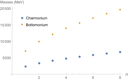
Figure 1: Masses of quarkonia states as a function of their radial excitation level.

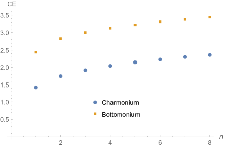
Figure 2: Configurational entropy (CE) of quarkonia as a function of the radial excitation level for $S$-wave resonances.

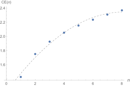
Figure 3: Configurational entropy (CE) as a function of the charmonium state radial excitation level (gray list plot); the dashed line represents a quadratic interpolation.

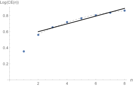
Figure 4: Logarithm of the configurational entropy (CE) as a function of the charmonium state radial excitation level (gray list plot); the black line refers to the linear regression and the dashed line represents a quadratic fit, both accomplished in the range $1<n\leq 8$.

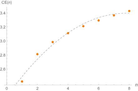
Figure 5: Configurational entropy (CE) as a function of the bottomonium state radial excitation level (orange list plot); the dashed line stands for a quadratic interpolation.

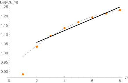
Figure 6: Logarithm of the configurational entropy (CE) as a function of the bottomonium state excitation level (orange list plot); the black line refers to the linear regression and the dashed line represents a quadratic fit, both accomplished in the range $1<n\leq 8$.

Figs. 1–6 show that the CE increases as value of the quarkonia radial excitation level increases, indicating that quarkonia states with lower excitation level have more dominance. By taking the logarithm of the configurational entropy as a function of the charmonium radial excitation level, the possibility of a scaling relation between the CE and the charmonium excitation level can be derived, which is illustrated in Fig. 4. In fact, the logarithm of the CE can be remarkably approximated by the linear function Log(CE($n$)) = $0.0483n+0.5025$, at least in the range $1<n\leq 8$, when we implement the linear regression procedure as a linear interpolation approach for modelling the relationship between the CE and the charmonium states excitation $n$ level. This linearization method is depicted as the black line in Fig. 4. The involved error underlying this linear approach is a tiny one, consisting of 4.1%. Besides, the logarithm of the CE can be also quadratically interpolated by the equation Log(CE($n$)) = $-0.0052n^{2}+0.1104n+0.3721$, plot into the dashed line in Fig. 4. The very small value of the quadratic coefficient in this last quadratic polynomial equation yields a quadratic scaling relation between the logarithm of the CE and charmonium states radial excitation level $n$, with an error of 0.2%, in the range $1<n\leq 8$.

Analogously, a similar analysis can be accomplished for the logarithm of the CE, as a function of the bottomonium state radial excitation $n$ level. Indeed, the logarithm of the CE can be linearly approximated by Log(CE($n$)) = $0.0318n+0.9938$, with an error of 4.6%, in the range $1<n\leq 8$. The linearization procedure implemented by the linear regression method in then illustrated by the black line in Fig. 5. Moreover, the logarithm of the CE can be quadratically interpolated by the equation Log(CE($n$)) = $-0.0037n^{2}+0.0693n+0.9151$, in the range $1<n\leq 8$. This quadratic fit has an error of 0.3%. Analogously to the charmonium states, the the logarithm of the CE has then a linear scaling with the bottomonium states radial excitation level.

V Concluding remarks and outlook

As discussed in Sects. I and II, recent studies indicate that the configurational entropy (CE) provides information about either the relative stability or dominance, among different states of a physical system. Here we have calculated the CE for heavy vector mesons by considering their supergravity holographic AdS/QCD duals. The results obtained for both bottomonium and charmonium states are that the CE increases with respect to the radial excitation level. This result is consistent with the observed fact that the higher excited states are in general less produced, or less abundant, that the lower states. Such a result reinforces the expectation of universality of the role of the CE. Our results here presented might be further generalized to other cases when the warp factor in Eq. (5) yields non-conformal deformations of the AdS₅ metric dePaula:2008fp . Strictly in the context of the CE, this model has been successfully applied, for providing information on the stability of the glueball states, as well as their relative dominance according to their spin, in Ref. Bernardini:2016qit . In addition, this model was also used to study light-flavor mesons Bernardini:2016hvx and might be adapted to encompass the setup developed in Sect. III. Nevertheless, it is still far beyond the proposed theme, regarding our results, and to carefully settle this setup has been revealing an intricate task.

References

- (1) M. Gleiser and N. Stamatopoulos, Phys. Lett. B 713, 304 (2012).
- (2) M. Gleiser and N. Stamatopoulos, Phys. Rev. D 86, 045004 (2012).
- (3) M. Gleiser and N. Graham, Phys. Rev. D 89, 083502 (2014).
- (4) M. Gleiser and D. Sowinski, Phys. Lett. B 747, 125 (2015).
- (5) A. E. Bernardini and R. da Rocha, Phys. Lett. B 762, 107 (2016).
- (6) A. E. Bernardini, N. R. F. Braga and R. da Rocha, Phys. Lett. B 765, 81 (2017).
- (7) G. Karapetyan, EPL 117, 18001 (2017).
- (8) G. Karapetyan, EPL 118, 38001 (2017).
- (9) N. R. F. Braga and R. da Rocha, Phys. Lett. B 767, 386 (2017).
- (10) C. O. Lee, Phys. Lett. B 772, 471 (2017).
- (11) M. Gleiser and D. Sowinski, Phys. Lett. B 727 (2013) 272.
- (12) M. Gleiser and N. Jiang, Phys. Rev. D 92, 044046 (2015).
- (13) R. Casadio and R. da Rocha, Phys. Lett. B 763, 434 (2016).
- (14) A. Gonçalves da Silva and R. da Rocha, Phys. Lett. B 774, 98 (2017).
- (15) A. Alves, A. G. Dias, R. da Silva, Braz. J. Phys. 47, 426 (2017).
- (16) A. Alves, A. G. Dias, R. da Silva, Physica 420, 1 (2015).
- (17) R. A. C. Correa and R. da Rocha, Eur. Phys. J. C 75, 522 (2015).
- (18) R. A. C. Correa, D. M. Dantas, C. A. S. Almeida and R. da Rocha, Phys. Lett. B 755, 358 (2016).
- (19) J. M. Maldacena, Int. J. Theor. Phys. 38, 1113 (1999).
- (20) S. S. Gubser, I. R. Klebanov and A. M. Polyakov, Phys. Lett. B 428, 105 (1998).
- (21) E. Witten, Adv. Theor. Math. Phys. 2, 253 (1998).
- (22) J. Polchinski and M. J. Strassler, Phys. Rev. Lett. 88, 031601 (2002).
- (23) H. Boschi-Filho and N. R. F. Braga, Eur. Phys. J. C 32, 529 (2004).
- (24) H. Boschi-Filho and N. R. F. Braga, JHEP 0305, 009 (2003).
- (25) A. Karch, E. Katz, D. T. Son and M. A. Stephanov, Phys. Rev. D 74, 015005 (2006).
- (26) S. J. Brodsky, G. F. de Teramond, H. G. Dosch and J. Erlich, Phys. Rept. 584, 1 (2015).
- (27) A. E. Bernardini, C. Dobrigkeit, J. Phys. G 29, 1439 (2003).
- (28) N. R. F. Braga, M. A. Martin Contreras and S. Diles, Phys. Lett. B 763, 203 (2016).
- (29) N. R. F. Braga, M. A. Martin Contreras and S. Diles, Eur. Phys. J. C 76, 598 (2016).
- (30) N. R. F. Braga and L. F. Ferreira, Phys. Lett. B 773, 313 (2017).
- (31) T. Matsui and H. Satz, Phys. Lett. B 178, 416 (1986).
- (32) N. R. F. Braga, L. F. Ferreira and A. Vega, arXiv:1709.05326 [hep-ph], to appear in Phys. Lett. B.
- (33) N. R. F. Braga, M. A. Martin Contreras and S. Diles, EPL 115, 31002 (2016).
- (34) Y. Liu and I. Zahed, Phys. Rev. D 95, no. 5, 056022 (2017).
- (35) Y. Liu and I. Zahed, Phys. Lett. B 769, 314 (2017).
- (36) K. A. Olive et al. [Particle Data Group Collaboration], Chin. Phys. C 38, 090001 (2014).
- (37) W. de Paula, T. Frederico, H. Forkel and M. Beyer, Phys. Rev. D 79, 075019 (2009).
- (38)