Partially Coherent Ptychography by Gradient Decomposition of the Probe

Abstract

Coherent ptychographic imaging experiments often discard over 99.9 % of the flux from a light source to define the coherence of an illumination. Even when coherent flux is sufficient, the stability required during an exposure is another important limiting factor. Partial coherence analysis can considerably reduce these limitations. A partially coherent illumination can often be written as the superposition of a single coherent illumination convolved with a separable translational kernel. In this paper we propose the Gradient Decomposition of the Probe (GDP), a model that exploits translational kernel separability, coupling the variances of the kernel with the transverse coherence. We describe an efficient first-order splitting algorithm GDP-ADMM to solve the proposed nonlinear optimization problem. Numerical experiments demonstrate the effectiveness of the proposed method with Gaussian and binary kernel functions in fly-scan measurements. Remarkably, GDP-ADMM produces satisfactory results even when the ratio between kernel width and beam size is more than one, or when the distance between successive acquisitions is twice as large as the beam width.

I Introduction

Ptychography is a popular imaging technique in scientific fields as diverse as condensed matter physics shi2016soft , cell biology giewekemeyer2010quantitative , materials science shapiro2014chemical and electronics holler2017high , among others. In a coherent ptychography experiment (Figure 1), a localized coherent X-ray probe (or illumination) $\omega$ scans through an specimen $u$, while the detector collects a sequence $J$ of phaseless intensities $f$ in the far field. The goal is to obtain a high resolution reconstruction of the specimen $u$ from the sequence of intensity measurements. In a discrete setting, $u\in\mathbb{C}^{n}$ is a 2D image with $\sqrt{n}\times\sqrt{n}$ pixels, $\omega\in\mathbb{C}^{\bar{m}}$ is a localized 2D probe with $\sqrt{\bar{m}}\times\sqrt{\bar{m}}$ pixels ($u$ and $\omega$ are both written as a vector by a lexicographical order), and $f_{j}=|\mathcal{F}(\omega\circ\mathcal{S}_{j}u)|^{2}$ is a stack of phaseless measurements  $f_{j}\in\mathbb{R}_{+}^{\bar{m}}~{}\forall 0\leq j\leq J-1$. Here $|\cdot|$ represents the element-wise absolute value of a vector, $\circ$ denotes the element-wise multiplication, and $\mathcal{F}$ denotes the normalized 2 dimensional discrete Fourier transform. Each $\mathcal{S}_{j}\in\mathbb{R}^{\bar{m}\times n}$ is a binary matrix that crops a region $j$ of size $\bar{m}$ from the image $u$.

In practice, as the probe is almost never completely known, one has to solve a blind ptychographic phase retrieval problem or probe retrieval thibault2009probe , as follows:

$${\text{ To find ~{}}\omega\in\mathbb{C}^{\bar{m}}\text{~{}and~{}}u\in\mathbb{C}^{n},~{}~{}}s.t.~{}~{}|\mathcal{A}(\omega,u)|^{2}=f,$$ (1)

where bilinear operators $\mathcal{A}:\mathbb{C}^{\bar{m}}\times\mathbb{C}^{n}\rightarrow\mathbb{C}^{m}$ and $\mathcal{A}_{j}:\mathbb{C}^{\bar{m}}\times\mathbb{C}^{n}\rightarrow\mathbb{C}^{\bar{m}}~{}\forall 0\leq j\leq J-1$, are denoted as follows:

$$\begin{split}\mathcal{A}(\omega,u):=&(\mathcal{A}_{0}^{T}(\omega,u),\mathcal{A}_{1}^{T}(\omega,u),\cdots,\mathcal{A}_{J-1}^{T}(\omega,u))^{T},\\ \mathcal{A}_{j}(\omega,u):=&\mathcal{F}(\omega\circ\mathcal{S}_{j}u),\end{split}$$

and $f:=(f^{T}_{0},f^{T}_{1},\cdots,f^{T}_{J-1})^{T}\in\mathbb{R}^{m}_{+}.$

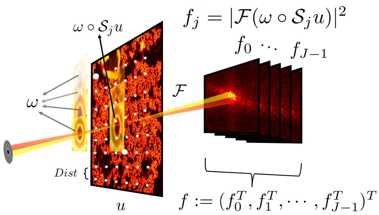
Figure 1: Ptychographic experiment (Far-field): A stack of intensities $f_{j}=|\mathcal{F}(\omega\circ\mathcal{S}_{j}u)|^{2}$ are collected, with $\omega$ being the localized coherent probe and $u$ being the image of interest (or specimen). The white dots on the image represent the center of probe or scanning lattice points with $Dist$ denoting the sliding distance between centers of two successive frames.

Coherent ptychographic imaging experiments often rely on apertures to define a coherent illumination. Research institutions around the world are investing considerable resources to produce brighter x-ray sources in order to overcome this limitation. Meanwhile, most of the x-ray photons generated are currently discarded by secondary apertures. Even when there is enough coherent flux, the stability required during an exposure is often another limiting factor. Both flux and stability limitations can be reduced using partial coherence analysis pelz2014fly ; deng2015continuous ; huang2015fly .

First, we briefly review the existing algorithmic work for partial coherence. In Fienup:93 the authors applied a gradient descent phase retrieval algorithm from incoherently averaged illuminations to compute the aberration of the Hubble space telescope. In clark2011simultaneous , the authors considered a constant quasi-monochromatic illumination on the sample (beam much larger than the sample), and derived a convolution based model using the mutual optical intensity as:

$$f_{pc}=f\ast\kappa,$$ (2)

where $f_{pc}$ is the measured partial coherent intensity, $f$ is the coherent intensity, $\ast$ denotes the convolution operator, and $\kappa$ is the kernel function (Fourier transform of the complex coherence function). Physically, the convolution kernel represents the combination of the detector response function and the angular spread of the illumination. It was solved by the alternating projection algorithm in clark2011simultaneous , when $\kappa$ is a Gaussian kernel function with free horizontal and vertical coherence length parameters. Burdet et al. burdet2015evaluation applied the above model to ptychographic imaging and proposed the Douglas-Rachford algorithm with a known Gaussian kernel function.

A more general description of a partially coherent wave field illuminating a specimen in a ptychography experiment was considered in thibault2013reconstructing , where the authors employed an orthogonal decomposition of the mutual coherence function wolf1982new to describe partially coherent measurement as follows:

$$f_{pc,j}=\sum\nolimits_{l=0}^{L-1}|\mathcal{A}_{j}(\omega_{l},u)|^{2},~{}\forall 0\leq j\leq J-1,$$ (3)

with $L$ orthogonal probes $\{\omega_{l}\}$, where $f_{pc}:=(f^{T}_{pc,0},\cdots,$ $f^{T}_{pc,J-1})^{T}$ is the measured intensity. The extended ptychographic iterative engine maiden2009improved was adopted to solve such model cao2016Modal . Experimental ‘fly-scan’ data with translational blur was successfully reconstructed using (3) by pelz2014fly ; deng2015continuous ; huang2015fly . However, it is important to note that such blur is a special case of a model that has many more degrees of freedom. Moreover, the physical interpretation of the multiple modes is unclear, and relationship with the coherence function is indirect.

Other existing studies focus mostly on (2), which only addressed blurring coherent intensities at the detector. In practice, the blur is dominated by the source dimensions and by the translation of the probe with respect to the image during an exposure pelz2014fly ; deng2015continuous . To the best of our knowledge, there is no algorithm in the literature to jointly recover the unknown image, probe, and coherence kernel function that exploits such property.

In this paper, we propose Gradient Decomposition of the Probe (GDP), a new forward model to characterize the partially coherent ptychography problem. The new model is based on coupling the experimental coherence widths with the variances of the kernel functions using the second order Taylor expansion to translate the probe. In the second part of this work we present GDP-ADMM: a novel fast iterative solver that jointly optimizes the image, the probe and the variance of the kernel function. The main benefits of the algorithm are listed below:

1. The approximation accuracy for a general partial coherent source is increased, while providing its coherent properties.

2. Subproblems can be solved using low computational and memory resources, and usually have close form.

3. It is insensitive to the coherence kernel and scanning step sizes, and achieves high SNR even when the data is contaminated by Poisson noise.

Numerical experiments show that satisfactory results with GDP-ADMM can be obtained even when the ratio between kernel and beam widths is more than one, or when the distance between successive acquisitions is almost twice as large as the beam width (Full Width Half Maximum-FWHM).

II Approximate forward model for partial coherence

Partially coherent illumination from standard microscopes can be written as the superposition of a single quasi-monochromatic coherent illumination convolved with separable angular and translational kernels GORI1978185 ; kim1986brightness ; coissonwalker86 ; coisson1997gauss . Translational convolution of the illumination is equivalent to translational motion during a scan while exposing the detector deng2015continuous . In other words, an extended incoherent source upstream of the lens can be viewed as the superposition, photon-by-photon, of a rapidly moving source demagnified by the lens onto the image plane. The demagnified source defines the degree of coherence of the probe, or the blurring kernel. Coherence and vibrations kernels can be combined into one, such that partially coherent ptychography imaging with coherence kernel function $\kappa$ in a continuous setting (same notations as in the discrete setting) is formulated as:

$$\int|\mathcal{F}_{x\rightarrow q}\left(\mathcal{S}_{j}u\left(x\right)\omega\left(x-y\right)\right)|^{2}\kappa(y)\mathrm{d}y=f_{pc,j}(q),$$ (4)

where $f_{pc}$ is the measured partial coherent intensity and $\mathcal{F}_{x\rightarrow q}$ is the normalized Fourier transform. When setting $\kappa$ to a binary function, the above model is exactly the same as fly-scan ptychography pelz2014fly ; deng2015continuous ; huang2015fly ; Setting $\kappa$ to the Dirac delta function reduces it to the coherent model (1). We remark that (4) is quite different from (2), since (4) illustrates the effects of blurring of images with respect to the probe, while (2) can be interpreted as blurring or binning multiple pixels at the detector.

Generally speaking, solving Eq. (4) is a non-linear ill-posed problem with an unknown kernel and there is no fast method to even compute the integral on the right hand side with known kernel, probe and images. In marchesini2013augmented ; tian2014multiplexed , the authors considered $L$ probes translated with weights $\{w_{l}\}$:

$$f_{pc,j}=\sum\limits_{l=0}^{L-1}w_{l}|{\mathcal{A}_{j}}(\mathcal{T}_{l}\omega,u)|^{2},~{}\forall 0\leq j\leq J-1,$$ (5)

with the translation operators $\{\mathcal{T}_{l}\},$ and partially coherent intensity $f_{pc}.$ However, those methods in marchesini2013augmented ; tian2014multiplexed cannot be directly applied to (4), since either the weights tian2014multiplexed or the probe marchesini2013augmented are assumed to be known in advance. Moreover, as coherence degrades, or the number of probes increases, their computation and memory costs would increase dramatically. Hence instead of solving (4) directly as in marchesini2013augmented , in the following sections we will reformulate the above model (4), and solve the related nonlinear optimization problem.

II.1 Gradient Decomposition of the Probe (GDP)

Following (4) and using the Taylor expansion of $\omega$, one has:

$$\begin{split}f_{pc,j}(q)=&\int\left|\mathcal{F}_{x\rightarrow q}\left(\mathcal{S}_{j}u(x)\left(\omega(x)-y^{T}\nabla\omega(x)\right.\right.\right.\\ &\left.\left.\qquad\qquad+\tfrac{1}{2}y^{T}\nabla^{2}\omega(x)y+\mathcal{O}(|y|^{3}))\right)\right|^{2}\kappa(y)\mathrm{d}y,\end{split}$$

where we assume that the third order derivatives are uniformly bounded, e.g.

$$\max_{\{\alpha\in\mathbb{N}^{2}:~{}|\alpha|=3\}}\max_{x\in\mathbb{C}^{2}}|\partial^{\alpha}\omega(x)|\leq C,$$ (6)

with a positive constant $C.$ It is easy to verify that this condition is satisfied when the illumination is generated by a small lens (with small aperture).

Consider a kernel function characterized by its moment expansion $m_{i_{1},i_{1}}=\int\kappa(y)y_{1}^{i_{1}}y_{2}^{i_{2}}\mathrm{d}y$, normalized with $m_{0,0}=1$, center of mass $(m_{1,0},m_{0,1})=(0,0)$, and second order moments $\sigma_{1}^{2}$, $\sigma_{2}^{2}$, and $\sigma_{12}$ ($\sigma_{1}^{2}\sigma_{2}^{2}-\sigma_{12}^{2}\geq 0$). We further assume that:

$$m_{i_{1},i_{2}}=0,\text{if~{}}\mathrm{mod}(i_{1}+i_{2},2)={1}.$$ (7)

The above relation holds if the kernel function is centro-symmetric with respect to the origin, i.e. $\kappa(-y_{1},-y_{2})=\kappa(y_{1},y_{2})$. For higher order moments, we also assume that

$$\int|y|^{k}\kappa(y)=\mathcal{O}(\max\{\sigma_{1},\sigma_{2}\}^{k}),\,k\geq 3.$$ (8)

Therefore, one has:

$$\small{\begin{split}f_{pc,j}(q)=&|\mathcal{A}_{j}(\omega+\tfrac{1}{2}(\sigma_{1}^{2}\nabla_{11}\omega+\sigma_{2}^{2}\nabla_{22}\omega+2\sigma_{12}\nabla_{12}\omega),u)|^{2}\\ &+\sigma_{1}^{2}|\mathcal{A}_{j}(\nabla_{1}\omega,u)|^{2}+\sigma_{2}^{2}|\mathcal{A}_{j}(\nabla_{2}\omega,u)|^{2}\\ &+\mathcal{O}(\int|y|^{3}\kappa(y)\mathrm{d}y).\end{split}}$$ (9)

More details of the above derivation can be found in Appendix B. In order to further simplify the partial coherence approximation we introduce a new variable $\tilde{\omega}$ (variance adjusted probe):

$$\tilde{\omega}:=\omega+\tfrac{1}{2}(\sigma_{1}^{2}\nabla_{11}\omega+\sigma_{2}^{2}\nabla_{22}\omega+{2\sigma_{12}\nabla_{12}\omega)},$$

and nonlinear operator $\mathcal{G}_{j}:\mathbb{C}^{\bar{m}}\times\mathbb{C}^{n}\times\mathbb{R}^{2}\rightarrow\mathbb{R}^{\bar{m}}_{+}$:

$$\begin{split}\mathcal{G}_{j}(\omega,u,\bm{\sigma})&:=|\mathcal{A}_{j}(\omega,u)|^{2}\\ &+\sigma_{1}^{2}|\mathcal{A}_{j}(\nabla_{1}\omega,u)|^{2}+\sigma_{2}^{2}|\mathcal{A}_{j}(\nabla_{2}\omega,u)|^{2},\end{split}$$ (10)

where $\bm{\sigma}:=(\sigma_{1},\sigma_{2})$. Neglecting high order terms $\mathcal{O}(\|\bm{\sigma}\|^{k}),$ $k\geq 3$, following (9), we obtain the approximate forward model:

$$\small{\begin{split}\mathrm{GDP:~{}~{}}f_{pc,j}\approx&\mathcal{G}_{j}(\tilde{\omega},u,\bm{\sigma}).\end{split}}$$ (11)

Remarks:

• The above assumptions hold if $\kappa$ is a Gaussian kernel function, which well approximates standard light sources such as synchrotrons kim1986brightness ; coissonwalker86 ; coisson1997gauss , SASE FELs saldin2008coherence , and others. When $\bm{\sigma}=(0,0),$ the above formula (11) reduces to the coherent model in (1).

• The variance adjusted probe $\tilde{\omega}$ incorporates second order effects (such as the covariance $\sigma_{12}$) into the illumination, while reducing the cost of computing the intensities using the forward model (11) compared to (5).

• If the probe $\omega$ has a support by a lens of finite size, $(\mathcal{F}\omega)(q)=0~{}\forall~{}q\in\Omega_{0}\subset\mathbb{R}^{2},$ then the same support applies to the variance adjusted probe $\forall~{}q\in\Omega_{0},$ $(\mathcal{F}\tilde{\omega})(q)=0$ due to the Fourier transform relationship:

  $$\begin{split}(\mathcal{F}\tilde{\omega})(q)&=\mathcal{F}((1+\tfrac{1}{2}\sigma_{1}^{2}\nabla_{11}+\tfrac{1}{2}\sigma_{2}^{2}\nabla_{22}+{\sigma_{12}\nabla_{12})\omega)(q)}\\ &=\left(1-\tfrac{1}{2}\sigma_{1}^{2}q_{1}^{2}-\tfrac{1}{2}\sigma_{2}^{2}q_{2}^{2}-\sigma_{12}q_{1}q_{2}\right)(\mathcal{F}\omega)(q),\\ &\forall~{}q=(q_{1},q_{2})\in\mathbb{R}^{2}.\end{split}$$

• Similarly to the decomposition model (3), GDP has three different modes $\{\tilde{\omega},\nabla_{1}\tilde{\omega},\nabla_{2}\tilde{\omega}\}$. The difference between them is that in the GDP model, two modes $\nabla_{l}\omega$ can be expressed by the first mode $\tilde{\omega}$ explicitly, while the multiple modes in the decomposition model (3) are only assumed to be orthogonal to each other wolf1982new ; thibault2013reconstructing . Such orthogonal constraint is essentially nonconvex, which is more difficult to handle and leads to more local minima as well.

III Fast iterative algorithm: GDP-ADMM

The amplitude based nonlinear optimization model can be established as:

$$\!\!\!\min\limits_{\tilde{\omega},u,\bm{\sigma}}\tfrac{1}{2}\sum\limits_{j=0}^{J-1}\big{\|}\sqrt{f_{pc,j}}-\sqrt{\mathcal{G}_{j}\left(\tilde{\omega},u,\bm{\sigma}\right)}\big{\|}^{2},$$ (12)

where $\|\cdot\|$ denotes the standard $L^{2}$ norm in Euclidean space. We remark that by introducing the new variable $\tilde{\omega}$, it is much easier to solve the subproblems of the nonlinear optimization model (12) with respect to $\bm{\sigma}$ than using the original formula (9).

The GDP based nonlinear optimization model (12) is nonconvex and non-differentiable. We are interested in designing a fast first order algorithm, whose subproblems can be easily implemented. The Alternating Direction Method of Multipliers (ADMM) Glowinski1989 has been successfully applied to large scale nonlinear and non-differential optimization problems arising from machine learning or computer vision, among other areas. The connection between ADMM, the Douglas-Rachford algorithm, and the popular Hybrid Input Output Fienup1982 for classical phase retrieval was discussed in Bauschke2003 ; Wen2012 . By introducing auxiliary variables $z_{l,j}\in\mathbb{C}^{\bar{m}}$, one has:

$$\begin{split}\min\limits_{\tilde{\omega},u,\bm{\sigma},z_{l,j}}&\tfrac{1}{2}\sum\limits_{j=0}^{J}\left\|\sqrt{f_{pc,j}}-\sqrt{\sum\limits_{l=0}^{2}|z_{l,j}|^{2}}\right\|^{2},\\ s.t.\qquad&z_{0,j}=\mathcal{A}_{j}(\tilde{\omega},u),z_{1,j}=\sigma_{1}\mathcal{A}_{j}(\nabla_{1}\tilde{\omega},u),\\ &\,z_{2,j}=\sigma_{2}\mathcal{A}_{j}(\nabla_{2}\tilde{\omega},u),~{}0\leq j\leq J-1.\end{split}$$ (13)

The corresponding augmented Lagrangian reads as:

$$\begin{split}&\mathcal{L}_{r}(\tilde{\omega},u,\{z_{l}\}_{l=0}^{2},\bm{\sigma},\{\Lambda_{l}\}_{l=0}^{2}):=\tfrac{1}{2}\sum\limits_{j}\left\|\sqrt{f_{pc,j}}-\tiny{\sqrt{\sum\limits_{l}|z_{l,j}|^{2}}}\right\|^{2}\\ &+r\Re(\langle z_{0}-\mathcal{A}(\tilde{\omega},u),\Lambda_{0}\rangle)+\tfrac{r}{2}\|z_{0}-\mathcal{A}(\tilde{\omega},u)\|^{2}\\ &+r\Re(\langle z_{1}-\mathcal{A}(\sigma_{1}\nabla_{1}\tilde{\omega},u),\Lambda_{1}\rangle)+\tfrac{r}{2}\|z_{1}-\mathcal{A}(\sigma_{1}\nabla_{1}\tilde{\omega},u)\|^{2}\\ &+r\Re(\langle z_{2}-\mathcal{A}(\sigma_{2}\nabla_{2}\tilde{\omega},u),\Lambda_{2}\rangle)+\tfrac{r}{2}\|z_{2}-\mathcal{A}(\sigma_{2}\nabla_{2}\tilde{\omega},u)\|^{2},\end{split}$$ (14)

with multipliers $\Lambda_{l}=(\Lambda^{T}_{l,0},\cdots,\Lambda^{T}_{l,J-1})^{T}\in{\mathbb{C}}^{m}$, $z_{l}=(z_{l,0}^{T},\cdots,z_{l,J-1}^{T})^{T}\in\mathbb{C}^{m}$, and the positive parameter $r,$ where $\langle\cdot,\cdot\rangle$ denotes the standard inner product in complex Euclidean space, and $\Re(\cdot)$ denotes the real part of a complex number. Briefly, the GDP-ADMM algorithm alternates minimization of the above augmented Lagrangian with respect to the variables $\omega,u,\sigma_{1},\sigma_{2}$, updates the multipliers $\Lambda_{l},l=0,1,2$, and repeats. In our previous work, ADMM was applied to coherent ptychographic imaging in Wen2012 ; chang2017blind . Here we propose a new, more robust variant of ADMM. It employs an additional proximal term added to the augmented Lagrangian: $\tfrac{\tau}{2}\|u-u^{k}\|^{2}_{M^{k}}$ to avoid division by zeros when minimizing with respect to $u$. The detailed description of GDP-ADMM can be found in Algorithm 1 (further details in Appendix A). The numerical results can be found in the following section. For simplicity, the gradient operator $\nabla_{1},\nabla_{2}$ in the numerical section is considered in a discrete setting, using the forward and finite difference operator with respect to $x,y$ directions.

Theoretical analysis about the convergence properties of this blind algorithm (to refine the probe, the image, and the coherence function variances during iterations) is likely to be very challenging. However, if the variances are known or fixed, convergence to the stationary point of the nonlinear optimization model (12) can be guaranteed by assuming that the iterative sequence is bounded and the parameter $r$ is sufficiently large chang2017blind .

Algorithm 1: GDP-ADMM

Initialization: Set $\tilde{\omega}^{0}=\mathcal{F}^{*}(\tfrac{1}{J}\sum\sqrt{f_{pc,j}}),$ $u^{0}=1,z_{0}^{0}=\mathcal{A}(\tilde{\omega}^{0},u^{0}),$ $\sigma^{0}_{1}=\sigma^{0}_{2}=1,$ $z^{0}_{0}=\mathcal{A}(\tilde{\omega}^{0},u^{0}),$ $z^{0}_{1}=\sigma^{0}_{1}\mathcal{A}(\nabla_{1}\tilde{\omega}^{0},u^{0}),$ $z^{0}_{2}=\sigma^{0}_{2}\mathcal{A}(\nabla_{2}\tilde{\omega}^{0},u^{0}),$ $\Lambda_{l}^{0}=0,k:=0,$ maximum iteration number $Iter_{Max},$ parameters $r$ and $\tau$.

output:x $u^{\star}:=u^{Iter_{Max}}$ and $\tilde{\omega}^{\star}:=\tilde{\omega}^{Iter_{Max}}.$for $k=0$ to $Iter_{Max}-1$

1. Compute $\tilde{\omega}^{k+1}$ by solving the linear system:

   $$\begin{split}&\tilde{\omega}^{k+1}=\left({N_{1}^{k}}\right)^{-1}\times c^{k},\end{split}$$ (15)

   using conjugate gradient method, where $N_{1}^{k}$, and $c^{k}$ are given in Eq. (22) (Appendix A).

2. Compute $u^{k+1}$ as

   $${\begin{split}u^{k+1}=\left(N_{2}^{k}+\tfrac{\tau}{r}M^{k}\right)^{-1}\times\left(b^{k}+\tfrac{\tau}{r}M^{k}u^{k}\right).\end{split}}$$ (16)

   with diagonal matrices $N_{2}^{k}$, $M^{k}$ and vector $b^{k}$ defined in Eq. (24), and (25) (see Appendix A).

3. Compute $z_{l}^{k+1}$ as:

   $$z^{k+1}_{l,j}=\dfrac{\sqrt{f_{pc,j}}+r\sqrt{\sum_{d=0}^{2}|\tilde{z}^{k+1}_{d,j}|^{2}}}{1+r}\circ\mathrm{sign}(\tilde{z}^{k+1}_{l,j}),$$ (17)

   with

   $$\begin{split}\mathrm{sign}(z_{l,j}):=&\tfrac{z_{l,j}}{\sqrt{\sum_{d=0}^{2}|z_{d,j}|^{2}}},\\ \tilde{z}^{k+1}_{0,j}=&\mathcal{A}(\tilde{\omega}^{k+1},u^{k+1})-\Lambda^{k}_{0},\\ \tilde{z}^{k+1}_{1,j}=&\sigma^{k}_{1}\mathcal{A}(\nabla_{1}\tilde{\omega}^{k+1},u^{k+1})-\Lambda^{k}_{1},\\ \tilde{z}^{k+1}_{2,j}=&\sigma^{k}_{2}\mathcal{A}(\nabla_{2}\tilde{\omega}^{k+1},u^{k+1})-\Lambda^{k+1}_{2}.\end{split}$$

4. Compute $\sigma_{l}^{k+1}$ as:

   $$\begin{split}&\sigma^{k+1}_{l}=\frac{\Re(\langle z^{k+1}_{l}+\Lambda^{k}_{l},\mathcal{A}(\nabla_{l}\tilde{\omega}^{k+1},u^{k+1})\rangle)}{\|\mathcal{A}(\nabla_{l}\tilde{\omega}^{k+1},u^{k+1})\|^{2}},~{}l=1,2.\\ \end{split}$$

5. Update the multipliers $\{\Lambda_{l}^{k+1}\}$ as

   $$\begin{split}&\Lambda_{0}^{k+1}=\Lambda_{0}^{k}+(z_{0}^{k+1}-\mathcal{A}(\tilde{\omega}^{k+1},u^{k+1}));\\ &\Lambda_{1}^{k+1}=\Lambda_{1}^{k}+(z_{1}^{k+1}-\mathcal{A}(\sigma^{k+1}_{1}\nabla_{1}\tilde{\omega}^{k+1},u^{k+1}));\\ &\Lambda_{2}^{k+1}=\Lambda_{2}^{k}+(z_{2}^{k+1}-\mathcal{A}(\sigma^{k+1}_{2}\nabla_{2}\tilde{\omega}^{k+1},u^{k+1})).\end{split}$$

IV Numerical experiments

The experimental setup of this section is introduced next. The reference specimen used is a complex valued image “Goldballs” marchesini2016sharp , of size $249\times 249$ pixels (Figure 2). The probe is an Airy disk of size $64\times 64$ pixels (Figure 2).

We compare the proposed GDP-ADMM (Appendix A) with the “fully-coherent” model by ADMM (FC-ADMM chang2017blind ). Both algorithms are executed with a maximum iteration number of 300. We measure the quality of recovery images by relative residuals as:

$${\begin{split}e_{fc}&=\tfrac{\left\|\sqrt{f}-|\mathcal{A}(\omega^{k},u^{k})|\right\|_{1}}{\big{\|}\sqrt{f}\big{\|}_{1}},\\ \!\!e_{pc}&=\tfrac{\left\|\sqrt{f}-\sqrt{\mathcal{G}\left(\tilde{\omega}^{k},u^{k},\bm{\sigma}^{{k}}\right)}\right\|_{1}}{\left\|\sqrt{f}\right\|_{1}},\\ \end{split}}$$

for FC-ADMM and GDP-ADMM respectively, where $\omega^{k},\tilde{\omega}^{k},u^{k},\bm{\sigma}^{k}$ are the iterative solutions, and $f$ is the measured intensity. The signal-to-noise ratio (SNR) is also measured:

$$\begin{split}&\mathrm{SNR}(u^{k},u_{true})=-20\min_{c\in\mathbb{C}}\log\frac{\|u^{k}-c~{}u_{true}\|}{\|u^{k}\|},\\ \end{split}$$

where $u_{true}$ is the ground truth of the image.

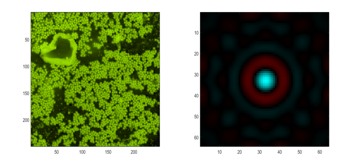
Figure 2: True image “Goldballs” marchesini2016sharp $249\times 249$ (left) and true probe (right) $64\times 64$, with “beam diameter” $D=7$ pixels (FWHM).

We show the performance of GDP-ADMM with the following Gaussian kernel function:

$$\kappa(y):=\tfrac{1}{2\pi\sigma_{1}\sigma_{2}}\exp(-\tfrac{y_{1}^{2}}{2\sigma_{1}^{2}}-\tfrac{y_{2}^{2}}{2\sigma_{2}^{2}}).$$ (18)

The discrete truncated Gaussian matrix is generated by fspecial in Matlab with variances $\sigma_{1},\sigma_{2}$ and support sizes $(4\sigma_{1}+1,4\sigma_{2}+1)$. We remark that the kernel width is $2\sqrt{2\log(2)}\times(\sigma_{1},\sigma_{2})\approx 2.35\times(\sigma_{1},\sigma_{2})$.

Simulated data is generated using raster grid scanning with sliding distance $\mathrm{Dist}=8$ pixels (slightly bigger than the beam width) as a default, and we incorporate the support constraint of the lens as in marchesini2016sharp . The parameter $r$ is selected manually with default value 0.2, and $\tau=1.01r$.

Noiseless data.

Following (4), the partially coherent intensity in a discrete setting is generated as

$$f_{pc,j}=\sum_{i}\kappa_{i}\big{|}\mathcal{F}((\mathcal{T}_{i}\omega)\circ\mathcal{S}_{j}u)\big{|}^{2},$$ (19)

with translation operator $\mathcal{T}_{i}$, discrete Gaussian weights $\{\kappa_{i}\}$, and periodical boundary condition for the probe. We conduct the first numerical experiment to explore the performance of the proposed algorithm with respect to different degrees of partial coherence by varying the variances $\sigma_{1},\sigma_{2}$, while keeping the beam width constant (the smaller the variances, the more coherent the data).

$\bm{\sigma}=(2,2)$	$(3,3)$	$(4,4)$	$(5,5)$
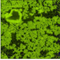
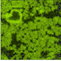
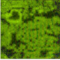
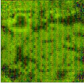
FC-ADMM
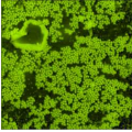
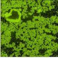
GDP-ADMM
$\bm{\sigma}=(4,0)$	$(5,0)$	$(6,0)$	$(7,0)$
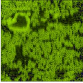
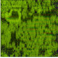
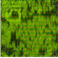
FC-ADMM
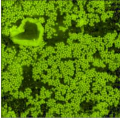
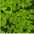
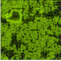
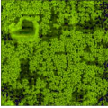
GDP-ADMM

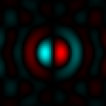
$\tilde{\omega}$	$\nabla_{1}\tilde{\omega}$	$\nabla_{2}\tilde{\omega}$

Figure 3: (First and third rows) reconstructed images of FC-ADMM, and (second and fourth rows) GDP-ADMM while varying $\bm{\sigma}$. (Bottom row) Probe with its three-modes $\tilde{\omega},\nabla_{1}\tilde{\omega},\nabla_{2}\tilde{\omega}$ from left to right recovered from the second row with $\bm{\sigma}=(4,4)$.

The reconstructed images can be seen in Figure 3, and the accuracy of the reconstructed results can be seen in Table 1. Figure 3 shows significant improvements when using GDP-ADMM compared to FC-ADMM. When coherence is very low (4th column), the visual quality of FC-ADMM drops, and small-scale features are completely lost. In comparison, with the same configuration, GDP-ADMM can still produce images containing significantly sharper large- and small-scale features. However the results by GDP-ADMM seem blurry when the kernel variance $\|\bm{\sigma}\|$ becomes too large, as can be seen from the fourth column of Figure (3). Table (1) shows the enhanced accuracy of GDP-ADMM compared to the coherent model: residuals are at least 50% percent smaller, and images with SNRs about twice as high. We also include the results of the recovered probe with its modes in Figure 3.

Table 1: Performance of GDP-ADMM and FC-ADMM. $e_{pc}$ and $e_{fc}$ are the residuals of GDP-ADMM and FC-ADMM respectively (the smaller, the better); $\mathrm{SNR}_{pc}$, $\mathrm{SNR}_{fc}$ are the SNRs for GDP-ADMM and FC-ADMM, respectively (the larger, the better).

$\bm{\sigma}$	(2,2)	(3,3)	(4,4)	(5,5)
$e_{fc}$	1.36E-1	1.88E-1	2.11E-1	2.20E-1
$e_{pc}$	2.60E-2	5.68E-2	8.95E-2	1.14E-1
$\mathrm{SNR}_{fc}$	14.78	9.53	6.14	4.37
$\mathrm{SNR}_{pc}$	23.73	18.83	13.02	8.37
$\bm{\sigma}$	(4,0)	(5,0)	(6,0)	(7,0)
$e_{fc}$	1.70E-1	1.89E-1	2.04E-1	2.14E-1
$e_{pc}$	5.62E-2	7.87E-2	9.76E-2	1.12E-1
$\mathrm{SNR}_{fc}$	11.47	9.42	7.61	5.64
$\mathrm{SNR}_{pc}$	19.83	16.39	13.46	10.94

Noisy data.

We consider Poisson noisy measurements as

$$f^{\mathrm{\,noise}}_{pc,j}=\tfrac{1}{\gamma}\mathrm{Poisson}(\gamma f_{pc,j}),$$

where $\gamma>0$ is used to control the noise level, and $f_{pc,j}$ is the clean partial coherent intensity data defined by (19). Figure 4 shows the recovered images at different noise levels. It can be seen that, as the noise level decreases (increasing $\gamma$), the quality of the results increases. We remark that when $\gamma=0.25$, the image in Figure 4 (a) is very blurry, which implies that it is more challenging to recover high quality images from partially coherent data contaminated by strong noise.

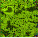
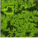
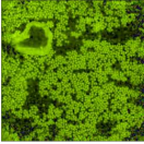
(a) $\mathrm{SNR}$=7.08	(b)10.17	(c) 11.30	(d) 12.35

Figure 4: Reconstructed images of GDP-ADMM while varying the level of Poisson noise, and the SNR with respect to the ground truth. From left to right: Noise level $\gamma=0.25,1,4,16$, (the larger $\gamma$, the weaker the noise). The corresponding SNRs of the data, defined by $\mathrm{SNR}(f^{noise},f)$, are 23.89, 29.87, 35.91, and 41.07.

Parameter $r$ and sliding distances.

The following experiment is conducted to study the influence of parameter $r$ by varying $r\in\{0.05,0.1,0.2,0.4,0.8\}$. See the convergence curve in Figure 5, where the change histories of the relative errors and SNRs with respect to iteration numbers are reported. One can readily see that with smaller parameter $r$, the algorithm tends to be unstable (see Figure 5 (b)). It is consistent with the condition for convergence guarantee in chang2017blind , where the parameter $r$ should be sufficiently large to make the augmented Lagrangian monotonically decrease. If the parameter is too big, the iterative solution could be trapped into the unsatisfactory local minima. Therefore, to gain optimal performance, a moderate $r$ should be used. We remark that although the parameter $r$ is selected manually, it can be applied to diverse cases with different degrees of partial coherence and sliding distances when fixing the kernel function.

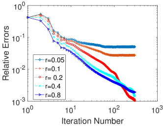
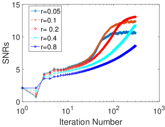
(a)	(b)

Figure 5: Performance influenced by parameter $r\in\{0.05,0.1,0.2,0.4,0.8\}$ of GDP-ADMM. (a) Relative errors $\tfrac{\|u^{k}-u^{k-1}\|}{\|u^{k}\|}$ of the iterative solution with respect to the iteration number; (b) SNRs of iterative solutions with respect to the iteration number.

In Figure 6 we conduct the tests with different sliding distances $\mathrm{Dist}\in\{4,6,8,12\}$, which determine the redundancy levels of the data. On one hand, inferred from the reported results, scanning with a smaller step size or $\mathrm{Dist}$ will help to increase the quality of the images. On the other hand, when $\mathrm{Dist}=12$ ( almost twice as large as the beam width), GDP-ADMM can still produce satisfactory results with clear small-scale features, showing the robustness of GDP-ADMM with respect to the redundancy of the measured data.

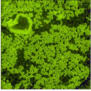
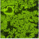
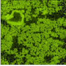
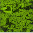
$\mathrm{Dist}$=4	6	8	12
SNR=15.93	14.54	13.02	8.96

Figure 6: Reconstructed images using GDP-ADMM with different sliding distances $\mathrm{Dist}$, Gaussian kernel function ($\bm{\sigma}=(4,4)$), and beam width $D=7$.

Proximal term.

In the following experiment we show the effect of the proximal term. We conduct tests comparing GDP-ADMM baseline with a variant that replaces the proximal term with a penalization term $\tfrac{\tau}{2}\|u\|^{2}$, i.e.

$$u^{k+1}=(N_{2}^{k}+\tfrac{\tau}{r}\mathbf{I})^{-1}b^{k},$$

with identity matrix ${\mathbf{I}}$ and $\tau=1\times 10^{-5}\times\|\mathrm{diag}(N_{2}^{k})\|_{\infty}\times r$ when solving Eq. (24), Appendix A. See the results in Figure 7. One can readily observe that with the help of the proximal term, the recovered images have cleaner boundaries (Figure 7 (b)) and higher SNR values (Figure 7 (d)). Moreover, GDP-ADMM is speeded up when using the proximal term, as shown by the convergence of the relative errors in Figure 7 (c).

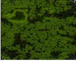
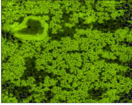
(a)	(b)
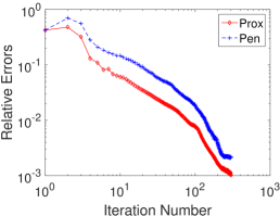
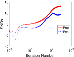
(c)	(d)

Figure 7: GDP-ADMM variant with penalization (“Pen”, (a)), versus GDP-ADMM baseline (“Prox”, (b)). The relative errors and SNRs are reported in (c) and (d), respectively. $\mathrm{Dist}=8$, $\bm{\sigma}=(4,4)$, beam width $D=7$.

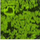
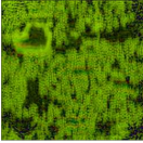
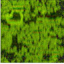
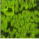
FC-ADMM
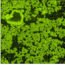
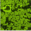
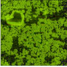
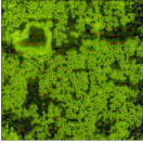
GDP-ADMM
$d=11$	13	15	17

Figure 8: Reconstructed images by FC-ADMM (top row) and GDP-ADMM (bottom) for fly-scan ptychography with varying kernel width $d$, beam width $D=7$, sliding distance $\mathrm{Dist}=8$.

Different kernels.

Previous experiments reported in this section are based on the Gaussian kernel function. Here we assess the performance of GDP-ADMM when using a binary kernel function for fly-scan ptychography deng2015continuous . Figure 8 shows the reconstructed images obtained by varying the kernel size $d$. Similarly to the case of Gaussian kernel function, GDP-ADMM displays a significant increase in visual quality. In the first row of Figure 8, the results produced by FC-ADMM are completely blurry. On the other hand, GDP-ADMM (second row of Figure 8) achieves much sharper overall results. One can also see the obvious decrease of the residual and increase of SNRs by GDP-ADMM in Table 2.

Similar improvements by GDP-ADMM can be obtained with other motion blur type kernel functions, however, due to page limitations, we do not provide further results. These results show that GDP-ADMM can be applied to partial coherence problems with more general kernel function.

Table 2: Fly-scan: Performance of GDP-ADMM and FC-ADMM. Here $d$ is the size of the binary kernel, and the beam width is $D=7$ pixels.

$d$	11	13	15	17
$e_{fc}$	2.00E-1	2.16E-1	2.29E-1	2.37E-1
$e_{pc}$	4.47E-2	6.46E-2	9.04E-2	1.16E-1
$\mathrm{SNR}_{fc}$	6.19	5.60	7.15	6.71
$\mathrm{SNR}_{pc}$	21.15	18.07	14.63	11.58

Runtime and memory performance

Finally we report the the computational performance of the GDP-ADMM algorithm on a machine with an Intel i7-5600U CPU and 16G RAM using Matlab. GDP-ADMM requires two additional modes and four additional variables $z_{1},z_{2}$ and $\Lambda_{1},\Lambda_{2}$ compared with FC-ADMM . Because of this, the memory cost and runtime of GDP-ADMM are in theory about three times as large as those of FC-ADMM per iteration. When computing the image in Figure 2, GDP-ADMM requires an average of 873MB of RAM and takes 655 seconds to compute, whereas FC-ADMM requires 344MB ad takes 218 seconds. These results are consistent with the previous theoretical estimate.

We further investigate the change histories of the SNRs for FC-ADMM and GDP-ADMM with respect to elapsed the time, and report the results in Figure 9. The SNR histories show that, FC-ADMM can recover better images in the first 50 seconds, but GDP-ADMM improves the image further after that. Hence, in order to accelerate the GDP-ADMM algorithm, we could use the iterative solution of FC-ADMM as the initialization for GDP-ADMM. We also emphasize that the runtime and memory requirements GDP-ADMM are insensitive to the variances and the support sizes of the kernel functions. It is important to note that, if we solve the problem directly following marchesini2013augmented , the probe and the weights in (5) in the case of the setting in Figure 3 (a)-(b), at most $(4\sigma_{1}+1)\times(4\sigma_{1}+1)=441$ translated probes for $\sigma_{1}=\sigma_{2}=5$ should be introduced, which requires much more memory and computation costs.

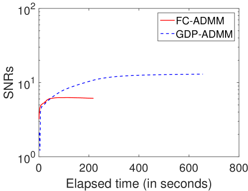
Figure 9: Histories of the SNRs changes for FC-ADMM and GDP-ADMM with respect to the elapsed time in seconds. $\sigma_{1}=\sigma_{2}=4$, Dist=8.

V Conclusions

In this paper, we propose Gradient Decomposition of the Probe (GDP), an efficient model that exploits translational kernel separability. The GDP model increases the approximation accuracy compared with the coherent model, and it holds for a general partial coherent source. We derive an optimization model coupling the variances of the kernel with the transverse coherence widths, and a fast and memory efficient proximal first order GDP-ADMM algorithm to solve the nonlinear optimization problem based on GDP. Numerical experiments demonstrate the effectiveness of such approximation in the case of Gaussian kernel function, and binary functions in fly-scanning schemes, showing that the proposed methods are suitable for general partially coherent sources.

However the results by GDP-ADMM seem blurry when inferred from the fourth column of Figure 3, and further improvement may be achieved by considering sparse prior, or using piecewise Taylor expansion series or other integration schemes. This will be subject of future work. Additional research directions to extend this work are: (i) consider partial coherence with framewise different variances $\bm{\sigma}_{j}$ when using scan geometries on irregular grids or spirals, (ii) combine translational blur at the sample with detector blur in Eq. (2) for near field ptychography. (ii) incorporate longitudinal coherence when using broadband illumination with chromatic aberrations of the probe, dispersion of the diffraction pattern enders2014ptychography , and spectral Kramers-Kronig dispersion across resonances hirose2017use .

VI Acknowledgments

This work was partially funded by the Center for Applied Mathematics for Energy Research Applications, a joint ASCR-BES funded project within the Office of Science, US Department of Energy, under contract number DOE-DE-AC03-76SF00098, and by the Advanced Light Source, which is a DOE Office of Science User Facility under contract no. DE-AC02-05CH11231.

Appendix A GDP-ADMM

Once the variables $\omega,u,z,\Lambda,\sigma$ are set, in the $(k+1)^{th}$ iteration the augmented Lagrangian is modified by adding a proximal term as follows:

$$\tilde{\mathcal{L}}^{k}_{r}(\tilde{\omega},u,z,\bm{\sigma},\Lambda)=\mathcal{L}_{r}(\tilde{\omega},u,z,\bm{\sigma},\Lambda)+\tfrac{\tau}{2}\|u-u^{k}\|^{2}_{M^{k}}\,,$$

where for simplicity we removed superscripts and subscripts, and $\|u\|_{M^{k}}^{2}=\langle M^{k}u,u\rangle$ is a positive semi-definite matrix $M^{k},$ defined by the approximated solution $\left(\tilde{\omega}^{k+1},u^{k},\{z_{l}^{k}\},\{\sigma_{l}^{k}\},\{\Lambda_{l}^{k}\}\right)$ in the $k^{th}$ iteration. We remark that with the help of an additional proximal term $\tfrac{\tau}{2}\|u-u^{k}\|^{2}_{M^{k}}$, the subproblem in Step 2 admits a unique solution. Below we demonstrate how to solve each subproblem.

$$\mbox{Step 1:~{}}\tilde{\omega}^{k+1}=\arg\min\limits_{\tilde{\omega}}\mathcal{L}_{r}(\tilde{\omega},u^{k},\{z^{k}_{l}\},\bm{\sigma}^{k},\{\Lambda^{k}_{l}\});$$ (20)

$$\mbox{Step 2:~{}}u^{k+1}=\arg\min\limits_{u}\tilde{\mathcal{L}}_{r}^{k}\left(\tilde{\omega}^{k+1},u,\{z^{k}_{l}\},\bm{\sigma}^{k},\{\Lambda^{k}_{l}\}\right);$$

$$\mbox{Step 4:~{}}\{z_{l}^{k+1}\}_{l=0}^{2}=\arg\min\limits_{\{z_{l}\}}\mathcal{L}_{r}(\tilde{\omega}^{k+1},u^{k+1},\{z_{l}\},\bm{\sigma}^{k},\{\Lambda^{k}_{l}\});$$

$$\mbox{Step 5:~{}}\bm{\sigma}^{k+1}=\arg\min_{\bm{\sigma}}\mathcal{L}_{r}(\tilde{\omega}^{k+1},u^{k+1},\{z^{k+1}_{l}\},\bm{\sigma},\{\Lambda^{k}_{l}\});$$

$$\mbox{Step 6:~{}}\Lambda_{0}^{k+1}=\Lambda_{0}^{k}+(z_{0}^{k+1}-\mathcal{A}(\tilde{\omega}^{k+1},u^{k+1}));$$

$$\mbox{~{}~{}~{}~{}~{}~{}~{}\quad}\Lambda_{1}^{k+1}=\Lambda_{1}^{k}+(z_{1}^{k+1}-\mathcal{A}(\sigma^{k+1}_{1}\nabla_{1}\tilde{\omega}^{k+1},u^{k+1}));$$

$$\mbox{~{}~{}~{}~{}~{}~{}~{}\quad}\Lambda_{2}^{k+1}=\Lambda_{2}^{k}+(z_{2}^{k+1}-\mathcal{A}(\sigma^{k+1}_{2}\nabla_{2}\tilde{\omega}^{k+1},u^{k+1}));$$

Step 1 involves finding the first order stationary point $\omega^{k+1}$ of the augmented Lagrangian which has the following form:

$$\begin{split}N_{1}^{k}\tilde{\omega}^{k+1}-c^{k}=0,\end{split}$$ (21)

with symmetric sparse matrix $N_{1}^{k}$ defined as:

$$\begin{split}N_{1}^{k}:=&\mathrm{diag}\left(\sum\limits_{j}\left|\mathcal{S}_{j}u^{k}\right|^{2}\right)\\ &+\sum\limits_{l=1}^{2}(\sigma^{k}_{l})^{2}\nabla_{l}^{T}\left(\mathrm{diag}\left(\sum\limits_{j}|\mathcal{S}_{j}u^{k}|^{2}\right)\nabla_{l}\right),\\ c^{k}:=&{\sum\limits_{j}\left(\mathcal{S}_{j}(u^{k})^{*}\circ\bar{z}^{k}_{0,j}+\sum\limits_{l=1}^{2}\sigma^{k}_{l}\nabla_{l}^{T}\left(\mathcal{S}_{j}(u^{k})^{*}\circ\bar{z}^{k}_{l,j}\right)\right),}\end{split}$$ (22)

and $\bar{z}^{k}_{l,j}:=\mathcal{F}^{*}(z^{k}_{l,j}+\Lambda^{k}_{l,j}).$ In this section, the gradient operator is given in a discrete setting for simplicity, where $\nabla_{1},\nabla_{2}$ represent the forward finite difference operator with respect to $x,y$ directions.

Step 2 is similar to Step 1, the closed form solution can be expressed as:

$$\left(N^{k}_{2}+\tfrac{\tau}{r}M^{k}\right)u^{k+1}-\left(b^{k}+\tfrac{\tau}{r}M^{k}u^{k}\right)=0,$$ (23)

with diagonal matrix $N_{2}^{k}$:

$$\begin{split}N_{2}^{k}:=&\mathrm{diag}\left(\sum\limits_{j}\mathcal{S}_{j}^{T}\left(|\tilde{\omega}^{k+1}|^{2}+\sum\limits_{l=1}^{2}\sigma^{2}_{l}|\nabla_{l}\tilde{\omega}^{k+1}|^{2}\right)\right),\\ b^{k}:=&\sum\nolimits_{j}\mathcal{S}_{j}^{T}\left((\tilde{\omega}^{k+1})^{*}\circ\bar{z}^{k}_{0,j}+\sum\limits_{l=1}^{2}\sigma^{k}_{l}\nabla_{l}(\tilde{\omega}^{k+1})^{*}\circ\bar{z}^{k}_{l,j}\right).\end{split}$$ (24)

Empirically, in order to avoid divisions by 0 when solving (23), set the matrix $M^{k}$ to a diagonal matrix with diagonal elements:

$$M^{k}(l,l):=\left\{\begin{split}&0,\qquad\qquad\qquad\,\text{if~{}}N_{2}^{k}(l,l)\geq\tfrac{1}{10}\|\mathrm{diag}(N_{2}^{k})\|_{\infty};\\ &\|\mathrm{diag}(N_{2}^{k})\|_{\infty}-\tfrac{r}{\tau}N_{2}^{k}(l,l),\,\text{otherwise.}\end{split}\right.$$ (25)

Step 3 can be expressed as the following problem:

$$\begin{split}\min_{\{z_{l,j}\}_{0\leq l\leq 2}^{0\leq j\leq J-1}}&\sum\nolimits_{j}\tfrac{1}{2}\left\|\sqrt{f_{pc,j}}-\sqrt{\sum\nolimits_{l}|z_{l,j}|^{2}}\right\|^{2}\\ &+\tfrac{r}{2}(\|z_{0}+\Lambda_{0}-\mathcal{A}(\tilde{\omega},u)\|^{2}\\ &+\|z_{1}+\Lambda_{1}-\mathcal{A}(\sigma_{1}\nabla_{1}\tilde{\omega},u)\|^{2}\\ &+\|z_{2}+\Lambda_{2}-\mathcal{A}(\sigma_{2}\nabla_{2}\tilde{\omega},u)\|^{2}),\end{split}$$

which can be solved independently with respect to each frame, hence one needs to consider:

$$\begin{split}\min_{\{z_{l,j}\}_{l=0}^{2}}&\tfrac{1}{2}\left\|\sqrt{f_{pc,j}}-\sqrt{\sum\nolimits_{l}|z_{l,j}|^{2}}\right\|^{2}\\ +&\tfrac{r}{2}\sum\nolimits_{l}\|z_{l,j}-\tilde{z}_{l,j}\|^{2}~{}\forall 0\leq j\leq J-1,\end{split}$$

where $\tilde{z}_{0,j}=\mathcal{A}_{j}(\tilde{\omega},u)-\Lambda_{0,j},\tilde{z}_{1,j}=\sigma_{1}\mathcal{A}_{j}(\nabla_{1}\tilde{\omega},u)-\Lambda_{1,j},\tilde{z}_{2,j}=\sigma_{2}\mathcal{A}_{j}(\nabla_{2}\tilde{\omega},u)-\Lambda_{2,j}.$ Similarly, it also has a closed form solution, see Eq. (17), Section III.

Step 4 requires solving a linear least square problem whose closed form solution is:

$$\begin{split}&\sigma_{l}=\frac{\Re(\langle z_{l}+\Lambda_{l},\mathcal{A}(\nabla_{l}\tilde{\omega},u)\rangle)}{\|\mathcal{A}(\nabla_{l}\tilde{\omega},u)\|^{2}}.\end{split}$$

Appendix B Derivation of (9)

$${\begin{split}\!f_{pc,j}(q)\!=&\!\int\!\!\left|\mathcal{F}_{x\rightarrow q}\left(\mathcal{S}_{j}u(x)\left(\omega(x)-y^{T}\nabla\omega(x)+\tfrac{1}{2}y^{T}\nabla^{2}\omega(x)y\right)\right)\right|^{2}\kappa(y)\mathrm{d}y+\mathcal{O}\left(\int|y|^{3}\kappa(y)\mathrm{d}y\right)\\ =&\!\int|\mathcal{F}_{x\rightarrow q}(\mathcal{S}_{j}u(x)(\omega(x)\!+\tfrac{1}{2}y^{T}\nabla^{2}\omega(x)y))|^{2}\kappa(y)\mathrm{d}y\!+\!\int|\mathcal{F}_{x\rightarrow q}(\mathcal{S}_{j}u(x)y^{T}\nabla\omega(x))|^{2}\kappa(y)\mathrm{d}y\!\!\\ &+\mathcal{O}\left(\int|y|^{3}\kappa(y)\mathrm{d}y\right)\\ \!\!&\!=\!\int\!|\mathcal{A}_{j}(\omega,u)+\tfrac{1}{2}y^{T}\mathcal{A}_{j}(\nabla^{2}\omega,u)y|^{2}\kappa(y)\mathrm{d}y\!+\int\!\!|y^{T}\mathcal{A}_{j}(\nabla\omega,u)|^{2}\kappa(y)\mathrm{d}y\!+\!\mathcal{O}(\int|y|^{3}\kappa(y)\mathrm{d}y)\!\!\\ =&|\mathcal{A}_{j}(\omega,u)|^{2}+2\Re\left(\mathcal{A}^{*}_{j}(\omega,u)\left(\tfrac{1}{2}\sigma_{1}^{2}\mathcal{A}_{j}(\nabla_{11}\omega,u)+\tfrac{1}{2}\sigma_{2}^{2}\mathcal{A}_{j}(\nabla_{22}\omega,u)+\sigma_{12}\mathcal{A}_{j}(\nabla_{12}\omega,u)\right)\right)\\ &+\mathcal{O}\left(\int|y|^{4}\kappa(y)\mathrm{d}y\right)+\sigma_{1}^{2}|\mathcal{A}_{j}(\nabla_{1}\omega,u)|^{2}+\sigma_{2}^{2}|\mathcal{A}_{j}(\nabla_{2}\omega,u)|^{2}+\mathcal{O}\left(\int|y|^{3}\kappa(y)\mathrm{d}y\right)\\ =&|\mathcal{A}_{j}(\omega,u)|^{2}\!+\!2\Re\left(\mathcal{A}^{*}_{j}(\omega,u)\mathcal{A}_{j}(\tfrac{1}{2}(\sigma_{1}^{2}\nabla_{11}\omega\!+\sigma_{2}^{2}\nabla_{22}\omega\!+2\sigma_{12}\nabla_{12}\omega),u)\right)\!\!\\ &+\sigma_{1}^{2}|\mathcal{A}_{j}(\nabla_{1}\omega),u)|^{2}+\sigma_{2}^{2}|\mathcal{A}_{j}(\nabla_{2}\omega,u)|^{2}+\mathcal{O}\left(\int|y|^{4}\kappa(y)\mathrm{d}y\right)+\mathcal{O}\left(\int|y|^{3}\kappa(y)\mathrm{d}y\right)\\ =&|\mathcal{A}_{j}(\omega+\tfrac{1}{2}(\sigma_{1}^{2}\nabla_{11}\omega+\sigma_{2}^{2}\nabla_{22}\omega+2\sigma_{12}\nabla_{12}\omega),u)|^{2}\\ &+\sigma_{1}^{2}|\mathcal{A}_{j}(\nabla_{1}\omega,u)|^{2}+\sigma_{2}^{2}|\mathcal{A}_{j}(\nabla_{2}\omega,u)|^{2}+\mathcal{O}(\int|y|^{3}\kappa(y)\mathrm{d}y),\end{split}}$$ (26)

where the first equality is based on:

$$\begin{split}&\int\left|\mathcal{F}_{x\rightarrow q}(\mathcal{S}_{j}u(x)(\omega(x)+\tfrac{1}{2}y^{T}\nabla^{2}\omega(x)y))-\mathcal{F}_{x\rightarrow q}(\mathcal{S}_{j}u(x)y^{T}\nabla\omega(x))\right|^{2}\kappa(y)\mathrm{d}y\\ =&\int\left(\left|\mathcal{F}_{x\rightarrow q}(\mathcal{S}_{j}u(x)(\omega(x)+\tfrac{1}{2}y^{T}\nabla^{2}\omega(x)y))\right|^{2}+\left|\mathcal{F}_{x\rightarrow q}(\mathcal{S}_{j}u(x)y^{T}\nabla\omega(x))\right|^{2}\right)\kappa(y)\mathrm{d}y\\ &-2\int_{y}\Re\left((\mathcal{F}_{x\rightarrow q}(\mathcal{S}_{j}u(x)(\omega(x)+\tfrac{1}{2}y^{T}\nabla^{2}\omega(x)y)))^{*}\mathcal{F}_{x\rightarrow q}(\mathcal{S}_{j}u(x)y^{T}\nabla\omega(x))\right)\kappa(y)\mathrm{d}y)\\ =&\int\left(|\mathcal{F}_{x\rightarrow q}(\mathcal{S}_{j}u(x)(\omega(x)+\tfrac{1}{2}y^{T}\nabla^{2}\omega(x)y))|^{2}+|\mathcal{F}_{x\rightarrow q}(\mathcal{S}_{j}u(x)y^{T}\nabla\omega(x))|^{2}\right)\kappa(y)\mathrm{d}y\\ &-2\Re\left(\int_{y}(\mathcal{A}_{j}(\omega,u)+y^{T}\mathcal{A}_{j}(\nabla^{2}\omega,u)y)^{*}(y^{T}\mathcal{A}_{j}(\nabla\omega,u))\kappa(y)\mathrm{d}y\right)\\ =&\int|\mathcal{F}_{x\rightarrow q}(\mathcal{S}_{j}u(x)(\omega(x)+\tfrac{1}{2}y^{T}\nabla^{2}\omega(x)y))|^{2}\mathrm{d}y+|\mathcal{F}_{x\rightarrow q}(\mathcal{S}_{j}u(x)y^{T}\nabla\omega(x))|^{2}\kappa(y)\mathrm{d}y\\ &-2\Re((\mathcal{A}_{j}(\omega,u))^{*}\mathcal{A}_{j}(\nabla\omega,u)\overbrace{\int_{y}y^{T}\kappa(y)\mathrm{d}y}^{\mathop{=0}{\eqref{thirdMZ}}}\\ &+\sum\limits_{1\leq i_{1},i_{2},i_{3}\leq 2}\mathcal{A}^{*}_{j}(\nabla_{i_{1},i_{2}}\omega,u)\mathcal{A}_{j}(\nabla_{i_{3}}\omega,u)\overbrace{\int_{y}y_{i_{1}}y_{i_{2}}y_{i_{3}}\kappa(y)\mathrm{d}y}^{\mathop{=0}{\eqref{thirdMZ}}})\\ =&\int\left(|\mathcal{F}_{x\rightarrow q}(\mathcal{S}_{j}u(x)(\omega(x)+\tfrac{1}{2}y^{T}\nabla^{2}\omega(x)y))|^{2}+|\mathcal{F}_{x\rightarrow q}(\mathcal{S}_{j}u(x)y^{T}\nabla\omega(x))|^{2}\right)\kappa(y)\mathrm{d}y,\end{split}$$

similarly, the first two terms of the fourth equality are derived by:

$${\begin{split}&\int|\mathcal{A}_{j}(\omega,u)+\tfrac{1}{2}y^{T}\mathcal{A}_{j}(\nabla^{2}\omega,u)y|^{2}\kappa(y)\mathrm{d}y\\ &=\int|\mathcal{A}_{j}(\omega,u)|^{2}\kappa(y)\mathrm{d}y+\Re\left(\mathcal{A}^{*}_{j}(\omega,u)\int y^{T}\mathcal{A}_{j}(\nabla^{2}\omega,u)y\kappa(y)\mathrm{d}y\right)\\ &\qquad+\int|\tfrac{1}{2}y^{T}\mathcal{A}_{j}(\nabla^{2}\omega,u)y|^{2}\kappa(y)\mathrm{d}y\\ &=\int|\mathcal{A}_{j}(\omega,u)|^{2}\kappa(y)\mathrm{d}y+\Re(\mathcal{A}^{*}_{j}(\omega,u)(\sigma_{1}^{2}\mathcal{A}_{j}(\nabla_{11}\omega,u)\\ &\qquad+\sigma_{2}^{2}\mathcal{A}_{j}(\nabla_{22}\omega,u)+2\sigma_{12}\mathcal{A}_{j}(\nabla_{12}\omega,u)))+\mathcal{O}\left(\int|y|^{4}\kappa(y)\mathrm{d}y\right),\end{split}}$$

and the third term of the fourth equality is derived by:

$${\begin{split}\int|y^{T}\mathcal{A}_{j}(\nabla\omega,u)|^{2}\kappa(y)\mathrm{d}y\mathop{=}^{\eqref{thirdMZ}}\sigma_{1}^{2}|\mathcal{A}_{j}(\nabla_{1}\omega,u)|^{2}+\sigma_{2}^{2}|\mathcal{A}_{j}(\nabla_{2}\omega,u)|^{2}.\end{split}}$$

References

- (1) H. H. Bauschke, P. L. Combettes, and D. R. Luke, Hybrid projection reflection method for phase retrieval, J. Opt. Soc. Amer. A, 20 (2003), pp. 1025–1034.
- (2) N. Burdet, X. Shi, D. Parks, J. N. Clark, X. Huang, S. D. Kevan, and I. K. Robinson, Evaluation of partial coherence correction in x-ray ptychography, Optics express, 23 (2015), pp. 5452–5467.
- (3) S. Cao, P. Kok, P. Li, A. M. Maiden, and J. M. Rodenburg, Modal decomposition of a propagating matter wave via electron ptychography, Phys. Rev. A, 94 (2016), p. 063621.
- (4) H. Chang and S. Marchesini, Blind ptychographic phase retrieval by globally convergent ADMM, submitted, (2017).
- (5) J. N. Clark and A. G. Peele, Simultaneous sample and spatial coherence characterisation using diffractive imaging, Applied Physics Letters, 99 (2011), p. 154103.
- (6) R. Coisson and S. Marchesini, Gauss–schell sources as models for synchrotron radiation, Journal of synchrotron radiation, 4 (1997), pp. 263–266.
- (7) J. Deng, Y. S. Nashed, S. Chen, N. W. Phillips, T. Peterka, R. Ross, S. Vogt, C. Jacobsen, and D. J. Vine, Continuous motion scan ptychography: characterization for increased speed in coherent x-ray imaging, Optics express, 23 (2015), pp. 5438–5451.
- (8) B. Enders, M. Dierolf, P. Cloetens, M. Stockmar, F. Pfeiffer, and P. Thibault, Ptychography with broad-bandwidth radiation, Applied Physics Letters, 104 (2014), p. 171104.
- (9) J. R. Fienup, Phase retrieval algorithms: a comparison, Appl. Opt., 21 (1982), pp. 2758–2769.
- (10) J. R. Fienup, J. C. Marron, T. J. Schulz, and J. H. Seldin, Hubble space telescope characterized by using phase-retrieval algorithms, Appl. Opt., 32 (1993), pp. 1747–1767.
- (11) K. Giewekemeyer, P. Thibault, S. Kalbfleisch, A. Beerlink, C. M. Kewish, M. Dierolf, F. Pfeiffer, and T. Salditt, Quantitative biological imaging by ptychographic x-ray diffraction microscopy, Proceedings of the National Academy of Sciences, 107 (2010), pp. 529–534.
- (12) R. Glowinski and P. L. Tallec, Augmented Lagrangian and operator-splitting methods in nonlinear mechanics, SIAM Studies in Applied Mathematics, Society for Industrial and Applied Mathematics (SIAM), Philadelphia, PA, 1989.
- (13) F. Gori and C. Palma, Partially coherent sources which give rise to highly directional light beams, Optics Communications, 27 (1978), pp. 185 – 188.
- (14) M. Hirose, K. Shimomura, N. Burdet, and Y. Takahashi, Use of kramers–kronig relation in phase retrieval calculation in x-ray spectro-ptychography, Optics Express, 25 (2017), pp. 8593–8603.
- (15) M. Holler, M. Guizar-Sicairos, E. H. Tsai, R. Dinapoli, E. Müller, O. Bunk, J. Raabe, and G. Aeppli, High-resolution non-destructive three-dimensional imaging of integrated circuits, Nature, 543 (2017), pp. 402–406.
- (16) X. Huang, K. Lauer, J. N. Clark, W. Xu, E. Nazaretski, R. Harder, I. K. Robinson, and Y. S. Chu, Fly-scan ptychography, Scientific reports, 5 (2015).
- (17) K.-J. Kim, Brightness, coherence and propagation characteristics of synchrotron radiation, Nuclear Instruments and Methods in Physics Research Section A: Accelerators, Spectrometers, Detectors and Associated Equipment, 246 (1986), pp. 71–76.
- (18) A. M. Maiden and J. M. Rodenburg, An improved ptychographical phase retrieval algorithm for diffractive imaging, Ultramicroscopy, 109 (2009), pp. 1256–1262.
- (19) S. Marchesini, H. Krishnan, D. A. Shapiro, T. Perciano, J. A. Sethian, B. J. Daurer, and F. R. Maia, Sharp: a distributed, gpu-based ptychographic solver, Journal of Applied Crystallography, 49 (2016), pp. 1245–1252.
- (20) S. Marchesini, A. Schirotzek, C. Yang, H.-t. Wu, and F. Maia, Augmented projections for ptychographic imaging, Inverse Problems, 29 (2013), p. 115009.
- (21) P. M. Pelz, M. Guizar-Sicairos, P. Thibault, I. Johnson, M. Holler, and A. Menzel, On-the-fly scans for x-ray ptychography, Applied Physics Letters, 105 (2014), p. 251101.
- (22) R. P. W. R. Coisson, Phase space distribution of brilliance of undulator sources, Proc.SPIE, 0582 (1986), pp. 0582 – 0582 – 8.
- (23) E. Saldin, E. Schneidmiller, and M. Yurkov, Coherence properties of the radiation from x-ray free electron laser, Optics Communications, 281 (2008), pp. 1179–1188.
- (24) D. A. Shapiro, Y.-S. Yu, T. Tyliszczak, J. Cabana, R. Celestre, W. Chao, K. Kaznatcheev, A. D. Kilcoyne, F. Maia, S. Marchesini, et al., Chemical composition mapping with nanometre resolution by soft x-ray microscopy, Nature Photonics, 8 (2014), pp. 765–769.
- (25) X. Shi, P. Fischer, V. Neu, D. Elefant, J. Lee, D. Shapiro, M. Farmand, T. Tyliszczak, H.-W. Shiu, S. Marchesini, et al., Soft x-ray ptychography studies of nanoscale magnetic and structural correlations in thin smco5 films, Applied Physics Letters, 108 (2016), p. 094103.
- (26) P. Thibault, M. Dierolf, O. Bunk, A. Menzel, and F. Pfeiffer, Probe retrieval in ptychographic coherent diffractive imaging, Ultramicroscopy, 109 (2009), pp. 338–343.
- (27) P. Thibault and A. Menzel, Reconstructing state mixtures from diffraction measurements, Nature, 494 (2013), p. 68.
- (28) L. Tian, X. Li, K. Ramchandran, and L. Waller, Multiplexed coded illumination for fourier ptychography with an led array microscope, Biomedical optics express, 5 (2014), pp. 2376–2389.
- (29) Z. Wen, C. Yang, X. Liu, and S. Marchesini, Alternating direction methods for classical and ptychographic phase retrieval, Inverse Probl., 28 (2012), p. 115010.
- (30) E. Wolf, New theory of partial coherence in the space–frequency domain. part i: spectra and cross spectra of steady-state sources, JOSA, 72 (1982), pp. 343–351.