Quantum thermodynamics of nanoscale steady states far from equilibrium

Abstract

We develop an exact quantum thermodynamic description for a noninteracting nanoscale steady state that couples strongly with multiple reservoirs. It is demonstrated that there exists a steady-state extension of the thermodynamic function that correctly accounts for the multiterminal Landauer-Büttiker formula of quantum transport of charge, energy or heat, via the nonequilibrium thermodynamic relations. Its explicit form is obtained for a single bosonic or fermionic level in the wide-band limit, and corresponding thermodynamic forces (affinities) are identified. Nonlinear generalization of the Onsager reciprocity relations are derived. We suggest that the steady-state thermodynamic function is also capable of characterizing the heat current fluctuations of the critical transport where the thermal fluctuations dominate. It is also pointed out that the suggested nonequilibrium steady-state thermodynamic relations seemingly persist for a spin-degenerate single level with local interaction.

I Introduction

Constructing a thermodynamic theory that applies consistently to nonequilibrium steady states has long been a theoretical challenge in many fields of science, not only in physics but also in chemistry or biology. Steady states differ from equilibrium states by being driven by the external environments (reservoirs) and accommodating finite flows that induce entropy production. Formulating thermodynamics for such irreversible systems is notoriously difficult; successes have been mainly achieved within the linear response theory, where various transport coefficients can be related to fluctuations in equilibrium Onsager and Machlup (1953); Kubo et al. (1985). Beyond the linear-response regime, a possible thermodynamic formulation has been anticipated for the steady states Oono and Paniconi (1998); Sasa and Tasaki (2006); Komatsu and Nakagawa (2008); Saito and Tasaki (2011); Hyldgaard (2012). Yet the theory has been largely unexplored so far, partly because basic concepts such as temperature and entropy get elusive and questioned when treating an open, irreversible system.

In recent years, it has been recognized that thermodynamic laws are consistent with quantum properties of open nanoscale systems, typically connected with multiple reservoirs with different chemical potentials and temperatures (Fig. 1). The emergence of thermodynamics is somewhat unexpected; the situation is opposite to the conventional thermodynamic limit, as it involves only a few particles, even a single one. The statistical ensemble average is replaced by quantum averaging, and the applicability of thermodynamics results from its quantum nature. Nanoscale systems provide a rare and novel opportunity to study the steady-state thermodynamics, without relying on any statistical ensemble hypothesis Anders and Esposito (2017).

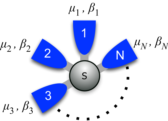
Figure 1: An open system (S) connected with multiple reservoirs with different inverse temperatures $\beta_{a}$ and chemical potentials $\mu_{a}$ for $a=1,\ldots,N$.

As a realization of nonequilibrium systems, a steady-state nanoscale system is notable because of its strong coupling with the reservoirs. One cannot rely on local equilibrium hypothesis to characterize a nano-system. Any temperature or chemical potential cannot be assigned to it a priori, except for a system coupled with a single reservoir. Strongly coupled reservoirs make effective dynamics non-Markovian with memory effect, and the Lindblad form of the master equation invalidated. The nonequilibrium density matrix is represented not by the standard Gibbs ensemble but by a generalized one (the MacLennan-Zubarev type) Zubarev et al. (1996); Tasaki and Takahashi (2006); Fujii (2007); Ness (2013). A consistent thermodynamic framework is nontrivial even for noninteracting transport. It has been striven for by many approaches Ludovico et al. (2014); Esposito et al. (2015); Topp et al. (2015); Bruch et al. (2016); Stafford and Shastry (2017), but it has not been fully disclosed so far.

In this paper, we develop a thermodynamic description of the steady state at nanoscale, entirely based on quantum mechanics. A steady-state extension of the Massieu-Planck function $\Phi_{\text{ss}}$, which is determined by normalization of the reduced density matrix, is singled out as a nonequilibrium thermodynamic function. One salient feature of this quantum construction is that the resulting thermodynamic function $\Phi_{\text{ss}}$ unavoidably becomes stationary in time because the steady-state density matrix is time-independent. It contrasts sharply with a naive expectation that a steady-state thermodynamic function might increase in time because it may include an increasing entropic contribution. Notwithstanding we will demonstrate that the function $\Phi_{\text{ss}}$ is viable to describe the steady-state properties far from equilibrium. To fully characterize the steady state, we also need to identify a correct set of parameters that control the steady state. A consistent choice of them includes local (inverse) temperature and chemical potential, $(\bar{\beta},\overline{\beta\mu})$, as well as various affinities $(A^{N}_{a},A^{E}_{a})$ that are thermodynamic forces to drive the system out of equilibrium [see Eqs. (21) for their definitions]. With these parameters, the significance of $\Phi_{\text{ss}}$ is compactly represented in the differential form:

$$d\Phi_{\text{ss}}=\bar{N}d(\overline{\beta\mu})-\bar{E}d\bar{\beta}+\frac{\hbar}{2\gamma}\sum_{a}\left(I_{a}\,dA^{N}_{a}+J_{a}\,dA^{E}_{a}\right),$$ (1)

where $\bar{N}$ or $\bar{E}$ is the average occupancy or energy of the system, while $I_{a}$ or $J_{a}$ is a nonlinear inflow of particle or energy from the reservoir $a$. The constant $\gamma$ is the total relaxation rate of the system. The relation (1) serves as a nonequilibrium extension of the thermodynamic relation of the Massieu-Planck function (see Appendix A). Being stationary in time, the function $\Phi_{\text{ss}}$ does not refer to the internal entropy. Yet $\Phi_{\text{ss}}$ characterizes the entropy production rate by

$$\frac{dS}{dt}=\frac{2\gamma}{\hbar}\sum_{a}\left(A^{E}_{a}\frac{\partial\Phi_{\text{ss}}}{\partial A^{E}_{a}}+A^{N}_{a}\frac{\partial\Phi_{\text{ss}}}{\partial A^{N}_{a}}\right).$$ (2)

These formulas (1)–(2) will be proved to be exact for a noninteracting single bosonic or fermionic level that couples linearly with multiple reservoirs. Moreover we argue the above thermodynamic structure Eqs. (1)–(2), found in a noninteracting steady state, persists even in a steady state of the model with local interaction, namely, the single-impurity Anderson model.

II Model and known results

The total Hamiltonian consists of $H=H_{S}+H_{R}+H_{SR}$, whose terms represent a nanoscale system (“quantum dot”), multiple reservoirs with different inverse temperatures $\beta_{a}$ and chemical potentials $\mu_{a}$ (for $a=1,\ldots,N$), and the linear coupling between the system and the reservoirs (see Fig. 1). They are

$$H_{S}=\epsilon_{d}\,d^{\dagger}d,$$ (3)

$$H_{R}=\sum_{a}\epsilon_{a\boldsymbol{k}}\,c_{a\boldsymbol{k}}^{\dagger}c_{a\boldsymbol{k}},$$ (4)

$$H_{SR}=\sum_{a,\sigma}\left(V_{da}\,d^{\dagger}c_{a\boldsymbol{k}}+V_{ad}\,c^{\dagger}_{a\boldsymbol{k}}d\right),$$ (5)

where $d^{\dagger}$ creates a particle with energy $\epsilon_{d}$ at the system and $c_{a\boldsymbol{k}}^{\dagger}$, with energy $\epsilon_{a\boldsymbol{k}}$ at the reservoir $a$. Particles can be bosonic or fermionic. We present the results for both cases simultaneously with composite signs (with the upper for bosonic; the lower for fermionic).

The presence of the reservoir makes the nanoscale system dissipative, inducing a finite resonant width $\gamma_{a}=\pi|V_{da}|^{2}\rho_{a}$ due to the reservoir $a$ (with its density of states $\rho_{a}$). Quantum transport across a noninteracting system can be solved exactly by several approaches, such as the scattering method, the equation-of-motion method, or the nonequilibrium Green function method. When we take the wide-band approximation, the inflow of particle $I_{a}$ or of energy $J_{a}$ from the reservoir $a$ is given by the Landauer-Büttier formula Landauer (1957); Sivan and Imry (1986); Meir and Wingreen (1992):

$$I_{a}=\frac{2}{\hbar}\sum_{b}\frac{\gamma_{a}\gamma_{b}}{\gamma}\int d\varepsilon\,\rho(\varepsilon)\,\left[f_{a}(\varepsilon)-f_{b}(\varepsilon)\right],$$ (6)

$$J_{a}=\frac{2}{\hbar}\sum_{b}\frac{\gamma_{a}\gamma_{b}}{\gamma}\int d\varepsilon\,\rho(\varepsilon)\varepsilon\,\left[f_{a}(\varepsilon)-f_{b}(\varepsilon)\right].$$ (7)

Here $\rho(\varepsilon)$ refers to the spectral function of the system,

$$\rho(\varepsilon)=\frac{\gamma/\pi}{(\varepsilon-\epsilon_{d})^{2}+\gamma^{2}};\quad\gamma=\sum_{a}\gamma_{a},$$ (8)

and $f_{a}(\varepsilon)=[e^{\beta_{a}(\varepsilon-\mu_{a})}\mp 1]^{-1}$ is the distribution function of the reservoir $a$. These currents are usually expressed by the transmission $\mathcal{T}_{ab}(\varepsilon)=4\pi\gamma_{a}\gamma_{b}\rho(\varepsilon)/\gamma$ between the reservoirs $a$ and $b$, but we prefer writing them in the above form. One can evaluate them analytically in terms of the digamma function [See Eqs. (60)–(61)]. Heat current flowing from the reservoir $a$ is defined by $J^{Q}_{a}=J_{a}-\mu_{a}I_{a}$. The average number $\bar{N}$ and energy $\bar{E}$ of the system are given by

$$\bar{N}=\int d\varepsilon\,\sum_{a}\frac{\gamma_{a}}{\gamma}\rho(\varepsilon)f_{a}(\varepsilon),$$ (9)

$$\bar{E}=\int d\varepsilon\,\sum_{a}\frac{\gamma_{a}}{\gamma}\rho(\varepsilon)\,\varepsilon\,f_{a}(\varepsilon).$$ (10)

We will show below that the steady-state thermodynamic function $\Phi_{\text{ss}}$, which is constructed quantum mechanically, correctly produces quantum transport equations (6)–(7) as well as local quantities (9)–(10) via the differential relation Eq. (1).

III The Massieu-Planck function

Analogous to an equilibrium system, our basic assumption is that the partition function which normalizes the density matrix bridges between a microscopic model and its thermodynamics. We suppose its steady-state extension is provided instead by normalizing the reduced density matrix $\hat{\varrho}_{\text{red}}$ of the relevant system. In treating the steady state, we find it advantageous to use the Massieu-Planck function Callen (1985), which is defined by the logarithm of the (effective) partition function.

III.1 Single-reservoir Massieu-Plank function

As for an open system that connects with a single reservoir with $\beta$ and $\mu$, the effective thermodynamics has long been investigated Feynman and Vernon (1963); Schotte and Schotte (1975); Caldeira and Leggett (1983); Weiss (2008); Hänggi et al. (2008); Adamietz et al. (2014). By recasting it, the single-reservoir Massieu-Planck function is found to be (see Appendix B)

$$\Phi_{1}(\beta,\beta\mu)=\mp\int^{\infty}_{-\infty}d\varepsilon\,\rho(\varepsilon)\ln\left[1\mp e^{-\beta(\varepsilon-\mu)}\right].$$ (11)

The energy integration actually diverges in the wide-band limit, so some regularization is needed. In Appendix C, we show the explicit analytical form of $\Phi_{1}(\beta,\beta\mu)$ with regularization, and examine its various thermodynamic properties that are independent of regularization. The physics of $\Phi_{1}$ is transparent; the level of the open nano-system acquires finite broadening due to coupling with the reservoir. We make a point of regarding $\Phi_{1}$ as a function of $\beta$ and $\beta\mu$, as they are parameters dual to particle number and energy. We stress that they are originally external parameters specified by the reservoir. The implication of $\beta$ and $\mu$ as thermodynamic parameters is somewhat blurred because the reduced density matrix $\varrho_{\text{red}}$ is no longer represented by the standard Gibbs ensemble.

III.2 Steady-state Massieu-Planck function

One can calculate the steady-state Massieu-Planck function $\Phi_{\text{ss}}$ that couples with multiple reservoirs by normalizing the reduced density matrix $\varrho_{\text{red}}$. As we work on noninteracting systems, the calculation can drastically be simplified by utilizing a Gaussian nature of $\hat{\varrho}_{\text{red}}$, in light of the Zubarev’s relevant distributions and nonequilibrium statistical operators Zubarev et al. (1996) (see also Chung and Peschel (2001); Peschel (2003); Dhar et al. (2012)). Asking $\bar{N}=\langle d^{\dagger}d\rangle$ to reproduce Eq. (9), we deduce that $\hat{\varrho}_{\text{red}}$ may well be represented in terms of relevant field operators $\psi_{a}(\varepsilon)$ and $\psi_{a}^{\dagger}(\varepsilon)$, satisfying

$$\left[\psi_{a}(\varepsilon),\psi_{a^{\prime}}^{\dagger}(\varepsilon^{\prime})\right]_{\mp}=\delta_{aa^{\prime}}\,\delta(\varepsilon-\varepsilon^{\prime}),$$ (12)

$$\left\langle\psi_{a^{\prime}}^{\dagger}(\varepsilon^{\prime})\psi_{a}(\varepsilon)\right\rangle=\delta_{aa^{\prime}}\,\delta(\varepsilon-\varepsilon^{\prime})\,f_{a}(\varepsilon),$$ (13)

$$d=\sum_{a}\int d\varepsilon\sqrt{\frac{\gamma_{a}}{\gamma}\rho(\varepsilon)}\,\psi_{a}(\varepsilon).$$ (14)

Then the function $\Phi_{\text{ss}}$ normalizes $\hat{\varrho}_{\text{red}}$ as

$$\hat{\varrho}_{\text{red}}=e^{-\Phi_{\text{ss}}-\sum_{a,\varepsilon}\beta_{a}(\varepsilon-\mu_{a})\psi_{a}^{\dagger}(\varepsilon)\psi_{a}(\varepsilon)},$$ (15)

where $\sum_{a,\varepsilon}(\cdots)=\sum_{a}\int d\varepsilon(\gamma_{a}/\gamma)\rho(\varepsilon)(\cdots)$ is the summation/integral over the energy shell and the reservoirs. Determining $\Phi_{\text{ss}}$ by imposing $\mathop{\mathrm{Tr}}\nolimits\hat{\rho}_{\text{red}}=1$ is equivalent to evaluating the functional determinant. A quick, symbolic way to evaluate it is

$$\exp\left(\Phi_{\text{ss}}\right)=\prod_{a,\varepsilon}\left[1\mp e^{-\beta_{a}(\varepsilon-\mu_{a})}\right]^{\mp 1},$$ (16)

$$\quad=e^{\mp\sum_{a,\varepsilon}\ln\left[1\mp e^{-\beta_{a}(\varepsilon-\mu_{a})}\right]}.$$ (17)

It expresses the steady-state Massieu-Planck function,

$$\Phi_{\text{ss}}=\sum_{a}\frac{\gamma_{a}}{\gamma}\Phi_{1}(\beta_{a},\beta_{a}\mu_{a}),$$ (18)

as a superposition of the single-reservoir contribution $\Phi_{1}(\beta_{a},\beta_{a}\mu_{a})$. Hence $\Phi_{\text{ss}}$ can be evaluated analytically. The manipulation of Eq. (16) is due to observing that $(\gamma_{a}/\gamma)\rho(\varepsilon)$ acts as (fractional) degeneracies satisfying $\sum_{a,\varepsilon}1=1$; such analytical continuation is validated because it correctly reproduces the single-reservoir result (11).

The relevant field operator $\psi_{a}^{\dagger}(\varepsilon)$ in Eqs. (12–15) has a clear physical meaning. One can construct the steady-state density matrix $\hat{\varrho}_{\text{ss}}$ of the total system (the system plus the reservoirs) Hershfield (1993); Fröhlich et al. (2003); Tasaki and Takahashi (2006); Oguri (2007); Ness (2013, 2014),

$$\hat{\varrho}_{\text{ss}}\propto\exp\left[-\sum_{a}\sum_{\boldsymbol{k}}\beta_{a}(\epsilon_{a\boldsymbol{k}}-\mu_{a})\psi_{a\boldsymbol{k}}^{\dagger}\psi_{a\boldsymbol{k}}\right],$$ (19)

where $\psi_{a\boldsymbol{k}}^{\dagger}=\Omega\,c_{a\boldsymbol{k}}^{\dagger}\Omega^{\dagger}$ is a scattering-state field of the reservoir $a$ that is defined by the Møller operator $\Omega$. The field $\psi^{\dagger}_{a\boldsymbol{k}}$ becomes a coherent superposition of fields $c^{\dagger}_{a\boldsymbol{k}}$ and $d^{\dagger}$. Accordingly, field $d$ is solved to be a superposition of the scattering fields involving all the reservoir fields, as in Eq. (14). It accounts for quantum coherence between the system and the reservoirs. The average density is $\langle\psi_{a\boldsymbol{k}}^{\dagger}\psi_{a\boldsymbol{k}}\rangle=f_{a}(\epsilon_{a\boldsymbol{k}})$, and the canonical (anti-)commutation relation is preserved. The relevant field $\psi_{a}(\varepsilon)$ is nothing but an energy representation of the scattering-state field $\psi_{a\boldsymbol{k}}$.

We cannot emphasize too much a novel and peculiar nature of Eq. (18). Although such a superposition is a common trait of quantum mechanics, Eq. (18) tells that the function $\Phi_{\text{ss}}$ that describes the irreversible steady state (with the increasing entropy) is unchanged in time and given by a superposition of $\Phi_{1}$’s of the single reservoirs, each of which refers to the entropy-preserving, reversible system. One may notice such a trait of superposition in the expression of average number $\bar{N}$ or energy $\bar{E}$ [Eq. (9) or (10)], but it is far from obvious that one can use $\Phi_{\text{ss}}$ to describe quantum transport $I_{a}$ and $J_{a}$. To fully disclose the steady-state thermodynamics, one needs to find what are relevant controlling parameters for it.

III.3 Affinities

Finding the correct set of appropriate controlling parameters arbitrary away from equilibrium is quite nontrivial, but it is imperative to establish the steady-state thermodynamic relations. The function $\Phi_{\text{ss}}$ of Eq. (18) depends on $2N$ independent external parameters $\{\beta_{a},\mu_{a}\}_{a=1,\ldots,N}$ specified by the reservoirs. Among them, we expect that two local parameters (temperature and chemical potential) regulate the average particle number and energy [Eqs. (9)–(10)], while all other $2N-2$ parameters (the difference of temperatures and/or chemical potentials) drive the system out of equilibrium and cause irreversible processes. The latter parameters are called thermodynamic forces or affinities. Among them, we will identify the relevant parameters $(\bar{\beta},\overline{\beta\mu},\{A^{N}_{a},A^{E}_{a}\})$ defined in Eqs. (21) below, which describe the quantum transport as well as thermodynamic properties. This constitutes our main result, with the steady-state thermodynamic function (18).

One can identify affinities and their associated currents by examining the internal entropy production rate Callen (1985). In the system we consider, it is balanced with the entropy inflow, so that we find

$$\frac{dS}{dt}=-\sum_{a}\beta_{a}\left(J_{a}-\mu_{a}I_{a}\right).$$ (20)

Its positivity follows because the distribution function $f_{a}(\varepsilon)$ is a decreasing function regarding $\beta_{a}(\varepsilon-\mu_{a})$ Fröhlich et al. (2003); Tasaki and Takahashi (2006); Nenciu (2007); Topp et al. (2015). The form of Eq. (20) tells us to introduce two types of affinities associated with each reservoir: chemical affinities $A^{N}_{a}$ to generate particle currents, which is a deviation of $\beta\mu$, and thermal affinities $A^{E}_{a}$ to generate energy currents, which is a deviation of $-\beta$. Those deviations must be defined from some reference values, $\bar{\beta}$ and $\overline{\beta\mu}$, which in turn regulate $\bar{N}$ and $\bar{E}$. We choose to introduce affinities for conserved currents of particle and energy rather than heat currents. The conservation laws are fulfilled by the condition $\sum_{a}\gamma_{a}A^{E}_{a}=\sum_{a}\gamma_{a}A^{N}_{a}=0$. Hence a pair of $A^{N,E}_{a}$ are redundant (see Appendix E for an explicit construction). All things considered, we come to make the following choice of local quantities $\bar{\beta}$ and $\overline{\beta\mu}$, and affinities:

$$A^{N}_{a}=\beta_{a}\mu_{a}-\overline{\beta\mu}; \overline{\beta\mu}=\sum_{a}\frac{\gamma_{a}}{\gamma}\,\beta_{a}\mu_{a},$$ (21a)

$$A^{E}_{a}=-\beta_{a}+\bar{\beta}; \bar{\beta}=\sum_{a}\frac{\gamma_{a}}{\gamma}\,\beta_{a}.$$ (21b)

Viewing $\Phi_{\text{ss}}$ of Eq. (18) as a function of the above set of parameters $(\bar{\beta},\overline{\beta\mu},\{A^{N}_{a},A^{E}_{a}\})$, it is now straightforward to find (see Appendix E for details)

$$\bar{N}=\frac{\partial\Phi_{\text{ss}}}{\partial(\overline{\beta\mu})};\quad\qquad\bar{E}=-\frac{\partial\Phi_{\text{ss}}}{\partial\bar{\beta}},$$ (22)

$$I_{a}=\frac{2\gamma}{\hbar}\frac{\partial\Phi_{\text{ss}}}{\partial A^{N}_{a}};\qquad J_{a}=\frac{2\gamma}{\hbar}\frac{\partial\Phi_{\text{ss}}}{\partial A^{E}_{a}}.$$ (23)

The expression Eq. (2) of the entropy production rate $dS/dt$ follows from Eqs. (20)–(23).

IV Discussion

IV.1 Local temperature

Our definition of local temperature $\bar{\beta}$ and chemical potential $\bar{\mu}=\overline{\beta\mu}/\bar{\beta}$ is motivated by the theoretical consistency of the thermodynamic formulation. Alternatively, one may probe local quantities by measurements such as the scanning thermal technique Majumdar (1999). Those probed quantities, $\beta_{p}$ and $\mu_{p}$, are determined by the no-flow condition of charge and energy when attaching the probe reservoir Meair et al. (2014); Stafford (2016); Shastry and Stafford (2016):

$$\int d\varepsilon\,\rho(\varepsilon)\,\varepsilon^{k}\left[\bar{f}(\varepsilon)-f_{p}(\varepsilon)\right]=0\quad\text{(for $k=0,1$)},$$ (24)

where $\bar{f}(\varepsilon)=\sum_{a}(\gamma_{a}/\gamma)f_{a}(\varepsilon)$ is the effective distribution of the reservoirs. In a general nonlinear setting far from equilibrium, parameters $\beta_{p}$ and $\mu_{p}$ may differ from $\bar{\beta}$ and $\bar{\mu}$. However, as for the linear deviation, the probed quantities $\beta_{p}$ and $\mu_{p}$ agree with $\bar{\beta}$ and $\bar{\mu}$, because the effective distribution $\bar{f}(\varepsilon)$ can be expanded as $\bar{f}(\varepsilon)\approx f_{p}(\varepsilon)+f^{\prime}_{p}(\varepsilon)[(\bar{\beta}-\beta_{p})\varepsilon-(\overline{\beta\mu}-\beta_{p}\mu_{p})]/\beta_{p}$. We also note that the scale $\bar{\mu}$ has played an important role of characterizing nonlinear electronic transport in the Kondo regime through an interacting dot Taniguchi (2014).

Explicit forms of local quantities and affinities in Eqs. (21) are outcomes of the wide-band approximation, which is well justified for quantum coherent transport through a nanostructure. If $\gamma_{a}$ were to acquire substantial energy dependence, one could nonetheless construct $\Phi_{\text{ss}}$ by generalizing Eq. (18) to take an energy-dependent superposition for each energy shell. However, it is quite nontrivial in this situation how to identify appropriate controlling parameters that enable us to construct the thermodynamic description.

IV.2 Maxwell relations and nonlinear generalization of the Onsager relations

The existence of the function $\Phi_{\text{ss}}$ that satisfies the differential form Eq. (1) has important consequences for the steady-state thermodynamic structure. One can derive various steady-state extensions of Maxwell relations by using the symmetry of second derivatives. For instance, we see the $\overline{\beta\mu}$ dependence of the current can be obtained by the chemical affinity dependence of the occupancy, as in

$$\frac{\partial^{2}\Phi_{\text{ss}}}{\partial A^{N}_{a}\partial(\overline{\beta\mu})}=\frac{\partial\bar{N}}{\partial A^{N}_{a}}=\frac{\hbar}{2\gamma}\cdot\frac{\partial I_{a}}{\partial(\overline{\beta\mu})}.$$ (25)

Many other relations are derived similarly. One can furthermore make a nonlinear generalization of the Onsager reciprocity relations by the symmetry $\partial^{2}\Phi_{\text{ss}}/\partial A^{E}_{a}\partial A^{N}_{a}$:

$$\frac{2\gamma}{\hbar}\cdot\frac{\partial\Phi_{\text{ss}}}{\partial A^{E}_{a}\partial A^{N}_{a}}=\frac{\partial I_{a}}{\partial A^{E}_{a}}=\frac{\partial J_{a}}{\partial A^{N}_{a}},$$ (26)

which is valid for nonlinear responses. In the linear-response limit (or the zero-affinity limit), the above gives the usual Onsager reciprocal relations between the cross coefficients.

IV.3 Implication in the interacting system

We have demonstrated that the function $\Phi_{\text{ss}}$ characterizes the steady state, based on a noninteracting transport model through a single level. Notwithstanding the validity of the thermodynamic structure Eqs. (1,2) seems to go beyond noninteracting systems to include a steady-state with local interaction. Let us consider the spin-degenerate fermionic single level with local interaction connecting with the multiple reservoirs, namely, the nonequilibrium single-impurity Anderson model. For that system, we can still derive the Landauer-Büttiker type formulas (6)–(7) by help of nonequilibrium Green functions Meir and Wingreen (1992); Lebanon and Schiller (2001); Sun and Guo (2001); Ţolea et al. (2009); Taniguchi (2014), where many-body effect is encapsulated only in the spectral function $\rho(\varepsilon)=-\mathop{\mathrm{Im}}\nolimits G^{R}(\varepsilon)/\pi$. Moreover, in the wide-band limit, the current conservation of charge and energy enforces Eqs. (9)–(10) even with interaction Taniguchi (2014). Note, the expression of $\bar{N}$ may be understood as a generalization of the Friedel sum rule Langer and Ambegaokar (1961); Langreth (1966); Rontani (2006) that holds at the zero temperature.

Therefore the structure of Eqs. (6)–(10) is intact even for the single-impurity Anderson model, in the the wide-band limit. Accordingly, we can deduce that a small deviation of $\Phi_{\text{ss}}$ should take a form of (1). Equivalently, it can be written as

$$d\Phi_{\text{ss}}=\mp\int d\varepsilon\,\rho(\varepsilon)\sum_{a}\frac{\gamma_{a}}{\gamma}\,d\log\left[1\mp e^{-\beta_{a}(\varepsilon-\mu_{a})}\right],$$ (27)

$$\quad=\int d\varepsilon\,\rho(\varepsilon)\sum_{a}\frac{\gamma_{a}}{\gamma}f_{a}(\varepsilon)\,d[\beta_{a}\mu_{a}-\beta_{a}\varepsilon].$$ (28)

The deviation $d[\beta_{a}\mu_{a}-\beta_{a}\varepsilon]$ is taken by regarding $(\bar{\beta},\overline{\beta\mu},A^{N}_{a},A^{E}_{a})$ as independent parameters, which gives Eq. (1). The form (28) is surprising, when one recalls that the local interaction makes the reduced density matrix $\hat{\varrho}_{\text{red}}$ non-Gaussian, and the spectral function $\rho(\varepsilon)$ dependent on the parameters. We suspect that there is some cancellation between the quadratic and quartic contributions, similarly to the nonequilibrium Ward identities Oguri (2005), because $\hat{\varrho}_{\text{ss}}$ still takes the Gaussian form Eq. (19) in terms of scattering-state fields, even for an interacting dot Hershfield (1993); Fröhlich et al. (2003); Tasaki and Takahashi (2006); Oguri (2007); Ness (2013, 2014). An actual mechanism is missing, though.

IV.4 Characterizing low-temperature heat current fluctuations

In the context of the large deviation approach to equilibrium statistical mechanics Ellis (2006), the free energy characterizes not only average quantities but also their fluctuations, being the cumulant generating function (CGF). Since the CGF of steady-state currents has been known Levitov and Lesovik (1993); Levitov et al. (1996); Saito and Dhar (2007), it would be desirable to see a connection with $\Phi_{\text{ss}}$, but a generic link between the CGF and $\Phi_{\text{ss}}$ is missing. Nevertheless we can show that the heat transport at low temperature give a concrete example of how $\Phi_{\text{ss}}$ is capable of characterizing the fluctuations.

The average heat current between two reservoirs (with different temperatures $\beta_{1,2}$ and the same chemical potential $\mu=0$) exhibits the universal behavior Schwab et al. (2000); Meschke et al. (2006),

$$J^{Q}\approx\frac{c\pi}{12\hbar}\left(\frac{1}{\beta_{1}^{2}}-\frac{1}{\beta_{2}^{2}}\right),$$ (29)

with the transmission coefficient $c=\mathcal{T}_{12}(\mu)$. It is known that the low-temperature current fluctuations are dominated by the thermal (Johnson-Nyquist) noise, even for the extreme nonequilibrium situation $\beta_{1}/\beta_{2}\gg 1$ Krive et al. (2001). Since one can connect the thermal noise with the thermal conductance, one may well say that $\Phi_{\text{ss}}$ characterizes those noises.

For perfect (or “critical”) transmission $c\approx 1$ which is realized for $\gamma_{1}$ = $\gamma_{2}$, one can develop conformal field theory to construct the CGF $F(\lambda)$ to characterize low-temperature heat current fluctuations Bernard and Doyon (2012, 2013); Bhaseen et al. (2015), which is found to be

$$F(\lambda)\approx\frac{c\pi}{12\hbar}\left[\frac{i\lambda}{\beta_{1}(\beta_{1}-i\lambda)}-\frac{i\lambda}{\beta_{2}(\beta_{2}+i\lambda)}\right].$$ (30)

It corresponds to the the low-temperature limit of Ref. [Saito and Dhar, 2007]. What is interesting in the present context is that Bernard and Doyon (2013) have noticed that the function $dF(\lambda)/d\lambda$ is related with the nonlinear heat current $J$ by what they call the extended fluctuation relations. Then by comparing with Eq. (1), we come to see that the CGF $F(\lambda)$ is directly given in terms of $\Phi_{\text{ss}}$:

$$F(\lambda) =\frac{\gamma}{\hbar}\left[\Phi_{\text{ss}}(\bar{\beta},A^{E}+2i\lambda)-\Phi_{\text{ss}}(\bar{\beta},A^{E})\right].$$ (31)

with $\bar{\beta}=(\beta_{1}+\beta_{2})/2$ and $A^{E}=-\beta_{1}+\beta_{2}$. Indeed, the low-temperature behavior of $\Phi_{\text{ss}}$ is readily evaluated from Eqs. (53) and (18) as

$$\Phi_{\text{ss}}\approx\frac{c\pi}{12\gamma}\left(\frac{1}{\beta_{1}}+\frac{1}{\beta_{2}}\right),$$ (32)

and putting it into Eq. (31) exactly reproduces Eq. (30). It is noted that the fluctuation theorem $F(\lambda)=F(iA^{E}-\lambda)$ is equivalent to the inversion symmetry $\Phi_{\text{ss}}(\bar{\beta},A^{E})=\Phi_{\text{ss}}(\bar{\beta},-A^{E})$ in this case.

V Conclusion

In summary, we have developed a thermodynamic description of the nonequilibrium steady state that connects with multiple reservoirs, and demonstrated that the steady-state Massieu-Planck function $\Phi_{\text{ss}}$ can characterize consistently its quantum transport properties of charge, energy or heat. The positive entropy production rate caused by irreversible processes is also characterized by $\Phi_{\text{ss}}$. We have evaluated explicitly for a single-level model that connects with multiple reservoirs, and argued that the same thermodynamic structure persists even for a steady state with local interaction, and that the heat current fluctuations are related to the function $\Phi_{\text{ss}}$ at low temperature.

Appendix A Thermodynamic relations of the equilibrium Massieu-Planck function

We recall some basic thermodynamic relations of the equilibrium Massieu-Planck function $\Phi_{\text{eq}}$, which is defined as the logarithm of the (grand) partition function Callen (1985). With a given thermodynamic potential $\Omega(T,\mu)$ as a function of the temperature $T$ and the chemical potential $\mu$, the function $\Phi_{\text{eq}}$ can be written as $\Phi_{\text{eq}}=-\Omega(T,\mu)/T$. Below we show how it is beneficial to regard $\Phi_{\text{eq}}$ as a function of the inverse temperature $\beta=1/T$ and $\beta\mu$. The volume of the system is irrelevant and ignored because we treat a nanoscale system.

Starting with the thermodynamic relation $d\Omega=-Nd\mu-SdT$, the thermodynamic relation of $\Phi_{\text{eq}}$ becomes

$$d\Phi_{\text{eq}}=-\Omega d\beta+N\beta d\mu-S\frac{d\beta}{\beta}=Nd(\beta\mu)-Ed\beta,$$ (33)

where we identify the entropy $S=-\beta\Omega+\beta(E-N\mu)$. One can check the above directly by making a quantum statistical construction of the partition function $e^{\Phi_{\text{eq}}}$. For noninteracting bosonic/fermionic particles with levels $\{\epsilon_{\alpha}\}$, one finds

$$\Phi_{\text{eq}}(\beta,\beta\mu)=\mp\sum_{\alpha}\ln\left[1\mp e^{-\beta(\epsilon_{\alpha}-\mu)}\right].$$ (34)

Then it is easy to see

$$\frac{\partial\Phi_{\text{eq}}(\beta,\beta\mu)}{\partial(\beta\mu)}\bigg{|}_{\beta} =\sum_{\alpha}f(\epsilon_{\alpha})=N,$$ (35)

$$\frac{\partial\Phi_{\text{eq}}(\beta,\beta\mu)}{\partial\beta}\bigg{|}_{\beta\mu} =-\sum_{\alpha}\epsilon_{\alpha}f(\epsilon_{\alpha})=-E,$$ (36)

$$\frac{\partial\Phi_{\text{eq}}(\beta,\beta\mu)}{\partial\beta}\bigg{|}_{\mu} =-\left(E-\mu N\right),$$ (37)

where $f(\epsilon)=[e^{\beta(\epsilon-\mu)}\mp 1]^{-1}$ is the distribution function. The entropy $S=-\partial\Omega/\partial T\big{|}_{\mu}$ is given by

$$S=\Phi_{\text{eq}}-\beta\frac{\partial\Phi_{\text{eq}}}{\partial\beta}\bigg{|}_{\mu}=\Phi_{\text{eq}}+\beta(E-\mu N).$$ (38)

The first equality means that $\Phi_{\text{eq}}$ is a Legendre transform of $S$ regarding $\beta$ with a fixed $\mu$. One finds the entropy $S$ taking a familiar Shannon-like form:

$$S=-\sum_{\alpha}\left\{f(\epsilon_{\alpha})\ln f(\epsilon_{\alpha})\mp\left[1\pm f(\epsilon_{\alpha})\right]\ln\left[1\pm f(\epsilon_{\alpha})\right]\right\}.$$ (39)

Appendix B Effective single-level thermodynamics coupled with a single reservoir

The calculation of the effective free energy of a single level $\epsilon_{d}$ that couples with a single reservoir (with the inverse temperature $\beta$ and the chemical potential $\mu$) has been long known for fermionic systems Schotte and Schotte (1975) as well as bosonic systems Weiss (2008); Hänggi et al. (2008); Adamietz et al. (2014). As in equilibrium, we then recast it to find the single-reservoir Massieu-Planck function $\Phi_{1}$ in Eq. (11) of the main text. Though the system coupled with a single reservoir no longer obeys the Gibbs ensemble, we may regard the reservoir’s parameters $\beta$ and $\mu$ as local thermal parameters of this open system, because of the thermodynamic relation,

$$N=\frac{\partial\Phi_{1}(\beta,\beta\mu)}{\partial(\beta\mu)}=\int^{\infty}_{-\infty}d\varepsilon\,\rho(\varepsilon)f(\varepsilon),$$ (40)

$$E=-\frac{\partial\Phi_{1}(\beta,\beta\mu)}{\partial\beta}=\int^{\infty}_{-\infty}d\varepsilon\,\rho(\varepsilon)\varepsilon f(\varepsilon).$$ (41)

Comparing between Eq. (34) and Eq. (11) in the main text, we see the spectral function $\rho(\varepsilon)$ play a role of degeneracy at each energy shell. Physical quantities are expressed simply by replacing the summation $\sum_{\alpha}(\cdots)$ by the energy integral $\int d\varepsilon\rho(\varepsilon)(\cdots)$. Particularly, the local entropy $S=\Phi_{1}+\beta(E-N\mu)$ becomes

$$S=-\int d\varepsilon\,\rho(\varepsilon)\left\{f(\varepsilon)\ln f(\varepsilon)\mp\left[1\pm f(\varepsilon)\right]\ln\left[1\pm f(\varepsilon)\right]\right\}.$$ (42)

This form of the entropy indicates that some entities having distribution $f(\varepsilon)$ is present at each energy shell, when putting it in the context of the information theory. This is why we have introduced field operators at each energy shell in the main text.

Appendix C Analytical form of $\Phi_{1}(\beta,\beta\mu)$ and regularization

For the Lorentzian spectrum of Eq. (8) in the main text, it is possible to obtain the analytical form of the single-reservoir Massieu-Planck function $\Phi_{1}$, hence the steady-state $\Phi_{\text{ss}}$ via Eq. (18) in the main text. The function $\Phi_{1}$ turns out to be divergent due to the zero-temperature contribution in the wide-band limit.  To suppress such divergence, we need to introduce a finite band width of the reservoir. The explicit form of $\Phi_{1}$ is useful to connect several different expressions found in the literature; it also clarifies the nature of the divergence and shows directly that physical quantities are independent of the regularization of such divergence.

A central role is played by the following integral formula

$$\int^{\infty}_{-\infty}\frac{d\varepsilon}{(\varepsilon-\epsilon_{d}+i\gamma)(e^{\beta(\varepsilon-\mu)}\mp 1)}$$

$$\quad=\int^{\infty}_{-\infty}\frac{\mp\theta(\mu-\varepsilon)\,d\varepsilon}{\varepsilon-\epsilon_{d}+i\gamma}-\frac{d}{dz}\log\mathcal{F}(z),$$ (43)

where the first term corresponds to the zero-temperature contribution while the second term, to the finite-temperature. The latter can be evaluated explicitly (see Gradshteyn et al. (2014) 3.415). We find it useful to express it by the complex function $\mathcal{F}(z)$ that is normalized by $\mathcal{F}(z)\to 1$ for large $|z|$:

$$\mathcal{F}(z)=\begin{cases}\displaystyle{\frac{\Gamma(z)\,z^{\frac{1}{2}-z}e^{z}}{\sqrt{2\pi}}},&\text{(B)},\\ \displaystyle{\frac{\sqrt{2\pi}z^{z}e^{-z}}{\Gamma(\frac{1}{2}+z)}},&\text{(F)},\end{cases}$$ (44)

as a function of the dimensionless complex parameter

$$z=x+iy=\frac{\beta}{2\pi}(\gamma+i\xi);\quad\xi=\epsilon_{d}-\mu.$$ (45)

The first term on the right-hand side of Eq. (43) is divergent, which we need to suppress by introduce finite band width of the reservoir,

$$\int^{\infty}_{-D}\frac{\mp\theta(\mu-\varepsilon)\,d\varepsilon}{\varepsilon-\epsilon_{d}+i\gamma}=\mp\log\big{(}z/z_{D}\big{)},$$ (46)

with the dimensionless cutoff $z_{D}=\beta[\gamma+i(D+\epsilon_{d})]/2\pi$. The formula (43) allows us to evaluate the average occupation number $N$ and energy $E$ in Eqs. (40)–(41) straightforwardly:

$$N(z)=\frac{1}{\pi}\mathop{\mathrm{Im}}\nolimits\left[\pm\log\big{(}z/z_{D}\big{)}+\frac{d}{dz}\log\mathcal{F}(z)\right],$$ (47)

$$\quad=\begin{cases}-\frac{1}{2}+\frac{1}{\pi}\mathop{\mathrm{Im}}\nolimits\left[\psi(z)+\frac{1}{2z}\right],&\text{(B)},\\ \frac{1}{2}-\frac{1}{\pi}\mathop{\mathrm{Im}}\nolimits\left[\psi(\frac{1}{2}+z)\right],&\text{(F)},\end{cases}$$ (48)

$$E(z)=\frac{1}{\pi}\mathop{\mathrm{Im}}\nolimits\left[(\epsilon_{d}-i\gamma)\left(\pm\log\big{(}z/z_{D}\big{)}+\frac{d}{dz}\log\mathcal{F}(z)\right)\right],$$ (49)

$$\quad=\begin{cases}\frac{1}{\pi}\mathop{\mathrm{Im}}\nolimits\left\{(\epsilon_{d}-i\gamma)\left[\psi(z)+\frac{1}{2z}-\log z_{D}\right]\right\},&\text{(B)},\\ -\frac{1}{\pi}\mathop{\mathrm{Im}}\nolimits\left\{(\epsilon_{d}-i\gamma)\left[\psi(\tfrac{1}{2}+z)-\log z_{D}\right]\right\},&\text{(F)}.\end{cases}$$ (50)

It is noted that while the average energy $E$ reduces to $\epsilon_{d}f(\epsilon_{d})$ in the isolated limit $\gamma\to+0$, it diverges for any finite $\gamma$ because of the zero-temperature contribution. Yet its finite-temperature contribution is well-defined.

One can construct the function $\Phi_{1}$ by integrating the above expression of $N$ or $E$. Those forms suggest that we may write it as

$$e^{\Phi_{1}}=A\;|\mathcal{F}(z)|^{2},$$ (51)

where $A$ is a factor coming from the zero-temperature contribution. Seeing $\Phi_{1}$ vanish at large $y$, one determines $A$ as

$$\log A=\pm 2\mathop{\mathrm{Re}}\nolimits\int^{z_{D}}_{z}\!\!dz^{\prime}\log(z^{\prime}/z_{D})=\left|\left(z_{D}/z\right)^{z}\right|^{\mp 2}.$$ (52)

This leads to the single-reservoir Massieu-Planck function,

$$\Phi_{1}(\beta,\beta\mu)=\begin{cases}\displaystyle{\ln\left|\frac{z^{\frac{1}{2}}\,\Gamma(z)}{\sqrt{2\pi}z_{D}^{z}\,e^{-z}}\right|^{2}},&\text{(B)},\\ \displaystyle{\ln\left|\frac{\sqrt{2\pi}z_{D}^{z}\,e^{-z}}{\Gamma(\tfrac{1}{2}+z)}\right|^{2}},&\text{(F)}.\end{cases}$$ (53)

It is always good to check the isolated limit $\gamma\to+0$. In this limit, we find

$$\left|\mathcal{F}(x+iy)\right|^{2} \>\to\>e^{\pm\pi(|y|-y)}\left(1\mp e^{-2\pi y}\right)^{\mp 1},$$ (54)

$$A\quad \>\to\>e^{\pm\pi(y-|y|)}.$$ (55)

Hence $e^{\Phi_{1}}\to\left[1\mp e^{-2\pi y}\right]^{\mp 1}$. This is nothing but the partition function of the isolated system Eq. (34).

In addition to $N$ and $E$, we can obtain various thermodynamic quantities by differentiating $\Phi_{1}(\beta,\beta\mu)$. They take a simple form in terms of the function $\mathcal{F}(z)$. For instance, the entropy $S$ becomes

$$S =\Phi_{1}-\beta\frac{\partial\Phi_{1}}{\partial\beta}\bigg{|}_{\mu}=2\mathop{\mathrm{Re}}\nolimits\bigg{[}\Big{(}1-z\frac{d}{dz}\Big{)}\log\mathcal{F}(z)\bigg{]},$$ (56)

$$=\begin{cases}2\mathop{\mathrm{Re}}\nolimits\left[\log\left(\frac{\Gamma(z)z^{\frac{1}{2}}}{\sqrt{2\pi}}\right)+z-\frac{1}{2}-z\psi(z)\right],&\text{(B)}\\ 2\mathop{\mathrm{Re}}\nolimits\left[\log\left(\frac{\sqrt{2\pi}}{\Gamma(\frac{1}{2}+z)}\right)-z+z\psi(\tfrac{1}{2}+z)\right].&\text{(F)}\end{cases}$$ (57)

The vanishing of $S$ at zero temperature follows from the fact $\mathcal{F}(z)\to 1$ for large $z$. The specific heat $C$ becomes

$$C =\beta^{2}\frac{\partial^{2}\Phi_{1}}{\partial\beta^{2}}\Big{|}_{\mu}=2\mathop{\mathrm{Re}}\nolimits\left[z^{2}\frac{d^{2}}{dz^{2}}\log\mathcal{F}(z)\right],$$ (58)

$$=\begin{cases}2\mathop{\mathrm{Re}}\nolimits\left[-\frac{1}{2}-z+z^{2}\psi^{\prime}(z)\right]&\text{(B)}\\ 2\mathop{\mathrm{Re}}\nolimits\left[z-z^{2}\psi^{\prime}(\tfrac{1}{2}+z)\right]&\text{(F)}\end{cases}.$$ (59)

The result of specific heat for fermionic systems agrees with that of Schotte and Schotte, 1975 (with $\xi=0$), while for the bosonic systems, it agrees with that of the damped harmonic oscillator Hänggi et al. (2008); Adamietz et al. (2014).

Appendix D Nonlinear current of charge, energy and heat

One can also find analytical expressions of nonlinear currents of particle, energy, or heat; they are well-defined and independent of the cutoff. From the thermodynamic relation (1) [or equivalently from Eqs. (6)–(7)] in the main text, we can write currents of particle and energy as

$$I_{a}=\frac{2}{\hbar}\sum_{b}\frac{\gamma_{a}\gamma_{b}}{\gamma}\left[N(z_{a})-N(z_{b})\right],$$ (60)

$$J_{a}=\frac{2}{\hbar}\sum_{b}\frac{\gamma_{a}\gamma_{b}}{\gamma}\left[E(z_{a})-E(z_{b})\right].$$ (61)

Here $N(z_{a})$ and $E(z_{a})$ are defined by Eqs. (47)–(50) for each reservoir by choosing $z_{a}=(\beta_{a}/2\pi)(\gamma+i\epsilon_{d}-i\mu_{a})$ with $\beta_{a}$ and $\mu_{a}$ of the reservoir [see Eq. (45)]. The difference of $N$ or $E$ is independent of cutoff. We see

$$N(z_{a})-N(z_{b})=\frac{1}{\pi}\mathop{\mathrm{Im}}\nolimits\left[\pm\log\Big{(}\frac{z_{a}}{z_{b}}　\Big{)}+\frac{\mathcal{F}^{\prime}(z)}{\mathcal{F}(z)}\bigg{|}^{z_{a}}_{z_{b}}\right],$$ (62)

$$E(z_{a})-E(z_{b})$$

$$\quad=\frac{1}{\pi}\mathop{\mathrm{Im}}\nolimits\left\{(\epsilon_{d}-i\gamma)\left[\pm\log\Big{(}\frac{\beta_{b}z_{a}}{\beta_{a}z_{b}}\Big{)}+\frac{\mathcal{F}^{\prime}(z)}{\mathcal{F}(z)}\bigg{|}^{z_{a}}_{z_{b}}\right]\right\}.$$ (63)

Therefore the finite-temperature contribution are written in terms of the digamma function $\psi(z)=\Gamma^{\prime}(z)/\Gamma(z)$ via Eq. (44). Likewise, heat current $J_{a}^{Q}=J_{a}-\mu_{a}I_{a}$ from the reservoir $a$ can be expressed analytically by using the above expressions.

Appendix E Derivation of Eq. (22) or (23)

Assigning an affinity that is associated with each current turns out delicate, particularly in multiterminal setting. Because of the current conservation, the inflow at the reservoir $a$ must involve outflows to other reservoirs. In order to establish Eqs. (22), (23), it is crucial to specify how one varies a relevant parameter by fixing others, as in equilibrium thermodynamics.

In the following, we choose to use $x_{a}$ for $\beta_{a}\mu_{a}$ or $-\beta_{a}$, to describe particle or energy transport, while we will introduce $y_{a}$ for affinities later. Adopting this notation, we write the steady-state Massieu-Planck function as $\Phi_{\text{ss}}=\sum_{a}(\gamma_{a}/\gamma)\Phi_{1}(x_{a})$, where $\Phi_{1}$ is defined by Eq. (11) in the text. Now we define the local parameter $\bar{x}$ and its affinity $y_{a}$ by

$$\bar{x}=\sum_{a=1}^{N}\frac{\gamma_{a}}{\gamma}x_{a};\quad y_{a}=x_{a}-\bar{x}.$$ (64)

Affinities $y_{a}$ satisfy the sum rule $\sum_{a}(\gamma_{a}/\gamma)y_{a}=0$. This comes from the condition that any variation of affinities does not affect $\bar{x}$. In this way, we map the $N$ parameters $\{x_{a}\}$ into $\bar{x}$ and $\{y_{a}\}$, where we can eliminate one of $\{y_{a}\}$. Alternatively, we can express $x_{a}$ as a function of $\bar{x}$ and the differences of $\{y_{a}\}$ by

$$x_{a}=\bar{x}+\sum_{b=1}^{N}\left(\delta_{ab}-\frac{\gamma_{b}}{\gamma}\right)y_{b}=\bar{x}+\sum_{b=1}^{N}\frac{\gamma_{b}}{\gamma}(y_{a}-y_{b}).$$ (65)

This parametrization is singled out by requiring to fix $\bar{x}$ by any variation of the $N$-independent parameters $\{y_{1},\ldots y_{N}\}$. Though we can safely cross out one of $\{y_{a}\}$ at any moment, we prefer retaining all of them for a symmetrical reason. In either way, we can obtain the currents fulfilling the current conservation by varying $y_{a}$ in the above.

Equation (22) or (23) can be derived by taking derivatives regarding $\bar{x}$ or $y_{a}$ by assuming $\bar{x}$ and $y_{a}$ are independent variables:

$$\bar{\mathcal{N}}=\frac{\partial\Phi_{\text{ss}}}{\partial\bar{x}}=\sum_{a=1}^{N}\frac{\gamma_{a}}{\gamma}\frac{\partial x_{a}}{\partial\bar{x}}\frac{\partial\Phi_{1}(x_{a})}{\partial x_{a}}=\sum_{a=1}^{N}\frac{\gamma_{a}}{\gamma}\mathcal{N}_{a},$$ (66)

$$\mathcal{I}_{a}=\frac{2}{\hbar}\frac{\partial\Phi_{\text{ss}}}{\partial y_{a}}=\frac{2\gamma}{\hbar}\sum_{b=1}^{N}\frac{\gamma_{b}}{\gamma}\frac{\partial x_{b}}{\partial y_{a}}\frac{\partial\Phi_{1}(x_{b})}{\partial x_{b}},$$ (67)

$$\quad=\frac{2\gamma}{\hbar}\sum_{b=1}^{N}\frac{\gamma_{b}}{\gamma}\left(\delta_{ab}-\frac{\gamma_{a}}{\gamma}\right)\mathcal{N}_{b}=\frac{2}{\hbar}\sum_{b=1}^{N}\frac{\gamma_{a}\gamma_{b}}{\gamma}\left(\mathcal{N}_{a}-\mathcal{N}_{b}\right),$$ (68)

Here we assign, for particle transport, $\bar{\mathcal{N}}=\bar{N}$, $\mathcal{I}_{a}=I_{a}$, and $\mathcal{N}_{a}=N(z_{a})$; for energy transport, $\bar{\mathcal{N}}=\bar{E}$, $\mathcal{I}_{a}=J_{a}$, and $\mathcal{N}_{a}=E(z_{a})$. The current conservation $\sum_{a}\mathcal{I}_{a}=0$ immediately follows from the above expression of $\mathcal{I}_{a}$.

Linear current $\mathcal{I}_{a}$ at terminal $a$ is proportional to $\gamma_{a}(x_{a}-\bar{x})=\gamma_{a}y_{a}$. Choosing the parametrization (65), it shows that positive affinity $y_{a}$ plays a role of inducing the inflow at the terminal $a$ but the outflows at all the other terminals, in the linear-response regime.

References

- Onsager and Machlup (1953) L. Onsager and S. Machlup, Phys. Rev. 91, 1505 (1953).
- Kubo et al. (1985) R. Kubo, M. Toda, and N. Hashitsume, Statistical Physics II, vol. 31 of Springer Series in Solid-State Sciences (Springer-Verlag, Berlin, 1985).
- Oono and Paniconi (1998) Y. Oono and M. Paniconi, Progress of Theoretical Physics Supplement 130, 29 (1998).
- Sasa and Tasaki (2006) S.-i. Sasa and H. Tasaki, Journal of Statistical Physics 125, 125 (2006).
- Komatsu and Nakagawa (2008) T. S. Komatsu and N. Nakagawa, Phys. Rev. Lett. 100, 030601 (2008).
- Saito and Tasaki (2011) K. Saito and H. Tasaki, Journal of Statistical Physics 145, 1275 (2011).
- Hyldgaard (2012) P. Hyldgaard, Journal of Physics: Condensed Matter 24, 424219 (2012).
- Anders and Esposito (2017) J. Anders and M. Esposito, New Journal of Physics 19, 010201 (2017).
- Zubarev et al. (1996) D. Zubarev, V. Morozov, and G. Röpke, Statistical Mechanics of Nonequilibrium Processes: Basic Concepts, Kinetic Theory, vol. 1 (Academie Verlag, Berlin, 1996).
- Tasaki and Takahashi (2006) S. Tasaki and J. Takahashi, Progress of Theoretical Physics Supplement 165, 57 (2006).
- Fujii (2007) T. Fujii, Journal of the Physical Society of Japan 76, 044709 (2007).
- Ness (2013) H. Ness, Phys. Rev. E 88, 022121 (2013).
- Ludovico et al. (2014) M. F. Ludovico, J. S. Lim, M. Moskalets, L. Arrachea, and D. Sánchez, Phys. Rev. B 89, 161306 (2014).
- Esposito et al. (2015) M. Esposito, M. A. Ochoa, and M. Galperin, Phys. Rev. Lett. 114, 080602 (2015).
- Topp et al. (2015) G. E. Topp, T. Brandes, and G. Schaller, EPL (Europhysics Letters) 110, 67003 (2015).
- Bruch et al. (2016) A. Bruch, M. Thomas, S. Viola Kusminskiy, F. von Oppen, and A. Nitzan, Phys. Rev. B 93, 115318 (2016).
- Stafford and Shastry (2017) C. A. Stafford and A. Shastry, The Journal of Chemical Physics 146, 092324 (2017).
- Landauer (1957) R. Landauer, IBM Journal of Research and Development 1, 223 (1957).
- Sivan and Imry (1986) U. Sivan and Y. Imry, Phys. Rev. B 33, 551 (1986).
- Meir and Wingreen (1992) Y. Meir and N. S. Wingreen, Phys. Rev. Lett. 68, 2512 (1992).
- Callen (1985) H. B. Callen, Thermodynamics and an introduction to thermostatistics (John Wiley & Son, New York, 1985), 2nd ed.
- Feynman and Vernon (1963) R. P. Feynman and F. L. Vernon, Annals of Physics 24, 118 (1963).
- Schotte and Schotte (1975) K. Schotte and U. Schotte, Physics Letters A 55, 38 (1975).
- Caldeira and Leggett (1983) A. O. Caldeira and A. J. Leggett, Ann. Phys. 149, 374 (1983).
- Weiss (2008) U. Weiss, Quantum Dissipative Systems, vol. 13 of Series in Modern Condensed Matter Physics (World Scientific, Singapore, 2008), 3rd ed.
- Hänggi et al. (2008) P. Hänggi, G.-L. Ingold, and P. Talkner, New Journal of Physics 10, 115008 (2008).
- Adamietz et al. (2014) R. Adamietz, G.-L. Ingold, and U. Weiss, The European Physical Journal B 87, 1 (2014).
- Chung and Peschel (2001) M.-C. Chung and I. Peschel, Phys. Rev. B 64, 064412 (2001).
- Peschel (2003) I. Peschel, Journal of Physics A: Mathematical and General 36, L205 (2003), arXiv:cond-mat/0212631.
- Dhar et al. (2012) A. Dhar, K. Saito, and P. Hänggi, Phys. Rev. E 85, 011126 (2012).
- Hershfield (1993) S. Hershfield, Phys. Rev. Lett. 70, 2134 (1993).
- Fröhlich et al. (2003) J. Fröhlich, M. Merkli, and D. Ueltschi, Ann. Henri Poincaré 4, 897 (2003).
- Oguri (2007) A. Oguri, Phys. Rev. B 75, 035302 (2007).
- Ness (2014) H. Ness, Phys. Rev. E 90, 062119 (2014).
- Nenciu (2007) G. Nenciu, Journal of Mathematical Physics 48, 033302 (2007).
- Majumdar (1999) A. Majumdar, Annual Review of Materials Science 29, 505 (1999).
- Meair et al. (2014) J. Meair, J. P. Bergfield, C. A. Stafford, and P. Jacquod, Phys. Rev. B 90, 035407 (2014).
- Stafford (2016) C. A. Stafford, Phys. Rev. B 93, 245403 (2016).
- Shastry and Stafford (2016) A. Shastry and C. A. Stafford, Phys. Rev. B 94, 155433 (2016).
- Taniguchi (2014) N. Taniguchi, Phys. Rev. B 90, 115421 (2014).
- Lebanon and Schiller (2001) E. Lebanon and A. Schiller, Phys. Rev. B 65, 035308 (2001).
- Sun and Guo (2001) Q.-f. Sun and H. Guo, Phys. Rev. B 64, 153306 (2001).
- Ţolea et al. (2009) M. Ţolea, I. V. Dinu, and A. Aldea, Phys. Rev. B 79, 033306 (2009).
- Langer and Ambegaokar (1961) J. S. Langer and V. Ambegaokar, Phys. Rev. 121, 1090 (1961).
- Langreth (1966) D. C. Langreth, Phys. Rev. 150, 516 (1966).
- Rontani (2006) M. Rontani, Phys. Rev. Let.. 97, 076801 (2006).
- Oguri (2005) A. Oguri, J. Phys. Soc. Jpn. 74, 110 (2005).
- Ellis (2006) R. S. Ellis, Entropy, Large Deviation and Statistical Mechanics, Reprint of the 1985 Edition (Springer, Berlin, 2006).
- Levitov and Lesovik (1993) L. S. Levitov and G. B. Lesovik, JETP Letters 58, 230 (1993).
- Levitov et al. (1996) L. S. Levitov, H. Lee, and G. B. Lesovik, J. Math. Phys. 37, 4845 (1996).
- Saito and Dhar (2007) K. Saito and A. Dhar, Phys. Rev. Lett. 99, 180601 (2007).
- Schwab et al. (2000) K. Schwab, E. A. Henriksen, J. M. Worlock, and M. L. Roukes, Nature 404, 974 (2000).
- Meschke et al. (2006) M. Meschke, W. Guichard, and J. P. Pekola, Nature 444, 187 (2006).
- Krive et al. (2001) I. V. Krive, E. N. Bogachek, A. G. Scherbakov, and U. Landman, Phys. Rev. B 64, 233304 (2001).
- Bernard and Doyon (2012) D. Bernard and B. Doyon, Journal of Physics A: Mathematical and Theoretical 45, 362001 (2012).
- Bernard and Doyon (2013) D. Bernard and B. Doyon, Journal of Physics A: Mathematical and Theoretical 46, 372001 (2013).
- Bhaseen et al. (2015) M. J. Bhaseen, B. Doyon, A. Lucas, and K. Schalm, Nat. Phys. 11, 509 (2015).
- Note (1) As for bosonic transport, we don’t usually need such regularization because we can set with the -integral spanning . Accordingly all the finite contributions are halved for that case.
- Gradshteyn et al. (2014) I. S. Gradshteyn, J. M. Ryzhjk, D. Zwillinger, and V. Moll, Table of Integrals, Series, and Products (Academic Press Inc., Amsterdam, 2014), 8th ed.