Reconstructing the Cosmic Expansion History with a Monotonicity Prior

Abstract

The cosmic expansion history, mapped by the Hubble parameter as a function of redshift, offers the most direct probe of the dark energy equation of state. One way to determine the Hubble parameter at different redshifts is essentially differentiating the cosmic age or distance with respect to redshift, which may incur large numerical errors with observational data. Taking the scenario that the Hubble parameter increases monotonically with redshift as a reasonable prior, we propose to enforce the monotonicity when reconstructing the Hubble parameter at a series of redshifts. Tests with mock type Ia supernova (SN Ia) data show that the monotonicity prior does not introduce significant biases and that errors on the Hubble parameter are greatly reduced compared to those determined with a flat prior at each redshift. Results from real SN Ia data are in good agreement with those based on ages of passively evolving galaxies. Although the Hubble parameter reconstructed from SN Ia distances does not necessarily provide more information than the distances themselves do, it offers a convenient way to compare with constraints from other methods. Moreover, the monotonicity prior is expected to be helpful to other probes that measure the Hubble parameter at multiple redshifts (e.g., baryon acoustic oscillations), and it may be generalized to other cosmological quantities that are reasonably monotonic with redshift.

1 Introduction

The Hubble parameter $H(z)$ maps the cosmic expansion history and is hence a crucial probe of the late-time accelerated expansion of the universe revealed by the luminosity distance-redshift relation of type Ia supernovae (SNe Ia) [1, 2]. Dark energy and modification to Einstein’s General Relativity are the two most discussed classes of models that try to explain the acceleration [3, 4, 5, 6, 7, 8, 9, 10, 11, 12, 13]. Dark energy and modified gravity models generally predict different growth history of the large-scale structure even if they produce the same cosmic expansion history. Therefore, one can potentially distinguish dark energy and modified gravity models by measuring both the expansion and growth histories [14, 15, 16]. Furthermore, under General Relativity, the Hubble parameter offers the most direct probe of the dark energy equation of state (EoS), whereas other observables are often integrals of $H^{-1}(z)$ or solved with differential equations involving $H(z)$. In modified gravity models, $H(z)$ is often still the most directly affected quantity by the specific modification to gravity theory. Measurements of the Hubble parameter are highly complementary to other types of measurements. Future surveys such as the Dark Energy Spectroscopic Instrument (DESI), the Euclid mission, and the Wide Field Infrared Survey Telescope (WFIRST) can determine $H(z)$ in different ways and cross-check with each other for robust tests on cosmology.

Despite its importance, only a few practical methods are available for measuring the Hubble parameter up to moderately high redshifts. Spectroscopic surveys of galaxies and quasars can determine $H(z)$ from line-of-sight baryon acoustic oscillations (BAOs) [17, 18, 19]. This will be a major undertaking of DESI, Euclid, and WFIRST. Another method is to essentially differentiate the redshift of passively evolving galaxies with respect to the age [20, 21], which is fairly independent of the cosmological model. However, noisy numerical differentiation together with observational errors and astrophysical modelling errors leads to rather large uncertainties [22, 20]. One can also differentiate SN Ia distances with respect to redshift to determine $H(z)$. Although such an analysis does not gain more information than already obtained from the distances, it is useful for cross-checking with other probes. We mention in passing that the redshift drift [23, 24] and the redshift difference between strongly lensed images of the same object [25] are sensitive to $H(z)$ as well. However, the required observations and analyses, if practical at all, are considerably more challenging.

Instead of differentiation, one can reconstruct the Hubble parameter from the age or distance data. Reconstruction may be parametric or non-parametric [26, 27]. With the former, the quantity of interest is described by a model with a small set of parameters, which works well if the model accurately reflects the underlying physics. However, one could inadvertently reach a wrong conclusion because the results are model-dependent. In non-parametric reconstruction, the quantity of interest is ideally represented by a complete set of orthogonal bases whose coefficients are determined by the data. An example would be a piecewise constant dark energy EoS in intervals of redshift or scale factor [28]. To reduce the number of degrees of freedom, one often truncates the basis set, and sometimes the basis functions are only approximately orthogonal in practice. An issue with non-parametric reconstruction is that the errors of the coefficients obtained usually increase with the number of basis functions used and eventually become proportional to the square root of the latter once the eigenmodes reach stable shapes [29]. Therefore, care needs to be taken when comparing results reconstructed from different datasets with different bases.

While reconstructing the Hubble parameter non-parametrically from SN Ia data with Markov Chain Monte Carlo (MCMC) sampling, we observe that many sample points have an $H(z)$ decreasing with redshift at least once in the whole history. This means that the total matter-energy density of the universe increased with time at some point in history under General Relativity, which would not happen in a flat universe with only radiation, dust, dark matter, and the cosmological constant, i.e., the $\Lambda$CDM model. Even if the cosmological constant is replaced by dark energy with a constant EoS (the $w$CDM model) or an EoS changing linearly with scale factor $a$ (the $w_{a}$CDM model [30, 31]), it is still unusual that $H(z)$ would decrease with $z$. We therefore take a step further proposing a monotonicity prior on $H(z)$, which requires the Hubble parameter to be an increasing function of redshift, or, equivalently, the total matter-energy density of the universe to always decrease with time under General Relativity. Tests with mock SN Ia data show that the monotonicity prior improves the Hubble parameter reconstruction without introducing significant biases. The reconstructed $H(z)$ from existing SN Ia samples is in good agreement with that from the ages of passively evolving galaxies.

The rest of this paper is organized as follows. Section 2 outlines the reconstruction method and discusses the monotonicity prior for the Hubble parameter. In section 3, we carry out tests on mock SN Ia samples and present the reconstructed $H(z)$ from existing SN Ia compilations – Supernova Cosmology Project (Union2.1) [32], Supernova Legacy Survey three-year sample (SNLS3) [33, 34, 35] and SDSS-II/SNLS3 Joint Light-curve Analysis (JLA) [36, 37]. An application to WFIRST is discussed briefly in section 3.4, and we summarize this work in section 4.

2 Reconstruction method

2.1 From Hubble parameter to SN Ia likelihood

We approximate the Hubble parameter as a function of redshift with a log-linear interpolation from its values at a series of redshifts, e.g.,

$$\hat{H}(z|\{z_{i},H_{i}\})=\exp\left[\ln H_{i}+\ln\left(\frac{H_{i+1}}{H_{i}}\right)\left(\frac{z-z_{i}}{z_{i+1}-z_{i}}\right)\right],$$ (2.1)

where $H_{i}=H(z_{i})$, $z_{i}\leq z<z_{i+1}$, and $\{z_{i}\}$ is covered by observational data. Following the usual notation, $H_{0}$ is the Hubble constant. Although eq. 2.1 results in a discontinuous deceleration function, which may not be physical, it has the advantage that a change to $H_{i}$ only affects interpolated values locally between $z_{i-1}$ and $z_{i+1}$. The interpolated deceleration and jerk functions can be made continuous with a cubic-spline. In such a case, there would not be much difference in the reconstructed results when the monotonicity prior is applied.

Because $H_{0}$ is degenerate with SN Ia peak absolute magnitude, one can only reconstruct the cosmic expansion function $E(z)=H(z)/H_{0}$ from SN Ia distances. Hence, the actual interpolation is performed with $\hat{E}(z|\{z_{i},E_{i}\})$, and we take the cosmic expansion rate $\bm{E}\equiv\{E_{i}\}$ as the target of reconstruction. When needed, we apply a prior on $H_{0}$ to recover the constraints on $\bm{H}\equiv\{H_{i}\}$ from those on $\{E_{i}\}$. Hereafter, we drop $\{z_{i},H_{i}\}$ and $\{z_{i},E_{i}\}$ in $\hat{H}(z)$ and $\hat{E}(z)$ respectively for convenience.

Under the assumption of an isotropic universe, the peak apparent magnitude $m_{\rm B}$ of a SN Ia at redshift $z$ is given by

$$m_{\rm B}(z) = 5\log_{10}\mathcal{D}_{\rm L}(z)+\mathcal{M}_{\rm B},$$ (2.2)

where $\mathcal{M}_{\rm B}\equiv M_{\rm B}+5\log_{10}\left[c/H_{0}\right]+25$ is the reduced SN Ia peak absolute magnitude, $c$ is the speed of light in vacuum, $M_{\rm B}$ is the SN Ia peak absolute magnitude in B-band, and $\mathcal{D}_{\rm L}(z)$ is the dimensionless luminosity distance

$$\mathcal{D}_{\rm L}(z)=\frac{1+z}{\sqrt{\Omega_{k}}}\sinh\left(\sqrt{\Omega_{k}}\int_{0}^{z}\frac{d\tilde{z}}{\hat{E}(\tilde{z})}\right),$$ (2.3)

with $\Omega_{k}$ being the curvature density parameter at present. For simplicity we assume a flat spacetime, i.e., $\Omega_{k}=0$, in this work.

The likelihood function of the SN Ia magnitudes for a given model is

$$\mathcal{L}(\bm{m}_{\rm B}^{\rm{obs}}|\bm{E},\bm{\theta}) = \frac{1}{(2\pi)^{N_{s}/2}|\mathbf{C}|^{1/2}}\exp\left[-\frac{1}{2}\Delta\bm{m}_{\rm B}^{\mathrm{T}}\cdot\mathbf{C}^{-1}\cdot\Delta\bm{m}_{\rm B}\right],$$ (2.4)

where $\Delta\bm{m}_{\rm B}$ is the difference between the observed peak apparent magnitude $\bm{m}_{\rm B}^{\rm{obs}}$ (after standardization) and the theoretical value $\bm{m}_{\rm B}^{\rm{th}}$ predicted by eq. (2.2), and $N_{s}$ is the size of the SN Ia sample in use. The observed peak apparent magnitude depends on a set of nuisance parameters $\bm{\theta}$, which are used in the peak-light magnitude corrections, including the light curve shape correction coefficient $\alpha$ and color correction coefficient $\beta$ (see table 1). The covariance matrix $\mathbf{C}$ has contributions from both statistical uncertainties and systematics. We defer the discussion of $\mathbf{C}$ until section 3.1.

From Bayes’ theorem one has the posterior distribution for $\bm{E}$ and $\bm{\theta}$

$$\mathcal{P}(\bm{E},\bm{\theta}|\bm{m}_{\rm B}^{\rm{obs}})\propto\mathcal{L}(\bm{m}_{\rm B}^{\rm{obs}}|\bm{E},\bm{\theta})\,\pi(\bm{E})\,\pi(\bm{\theta}),$$ (2.5)

where $\pi(\bm{E})$ and $\pi(\bm{\theta})$ are the priors, and $\bm{E}$ and $\bm{\theta}$ are assumed to be uncorrelated. The reduced peak absolute magnitude $\mathcal{M}_{\mathrm{B}}$ is absorbed into $\bm{\theta}$ for notational simplicity. The normalization factor or the Bayesian evidence of the posterior distribution is useful for model selection [38, 39]. For our purpose, we treat it as an irrelevant constant.

2.2 Monotonicity prior

When a flat prior (also known as non-informative prior) is applied to the parameters, one gets many unusual sample points that have an expansion rate decreasing with redshift at some point. Expansion histories represented by these sample points are unlikely to have happened in the concordant $\Lambda$CDM cosmological model or its extensions such as the $w$CDM and $w_{a}$CDM models. To remove these rather unphysical sample points, we propose to apply a monotonicity prior on the Hubble parameter, which requires $H(z)$ to be a function monotonically increasing with redshift. It is equivalent to the Null Energy Condition in a flat universe [40, 41]. Since $H(z)=H_{0}\,E(z)$, the prior on the Hubble parameter may be written as a product of two uncorrelated parts: $\pi(\bm{H})=\pi(H_{0})\,\pi(\bm{E})$. Thus the monotonicity prior reads

$$\pi(\bm{E})=\left\{\begin{array}[]{lll}1,&{}&\mbox{$E_{i}\leq E_{i+1}$ for all $i$},\\ 0,&{}&\mbox{otherwise}.\end{array}\right.$$ (2.8)

To obtain constraints on the Hubble parameter, one maps the reconstructed cosmic expansion rate $\bm{E}$ into Hubble rate $\bm{H}$ by multiplying every sample point in the $\bm{E}$ chains with a randomly sampled $H_{0}$ from a prior distribution $\pi(H_{0})$, e.g., ref. [42]. In appendix A we provide an equivalent form of the monotonicity prior that is more efficient for MCMC sampling.

In the $\Lambda$CDM model, the expansion function is $E(z;\Omega_{\rm m})=\sqrt{\Omega_{\rm m}(1+z)^{3}+(1-\Omega_{\rm m})}$, where $\Omega_{\rm m}$ is the matter density parameter defined as the ratio of today’s matter density to the critical density $\rho_{\rm{crit}}\equiv 3H^{2}_{0}/8\pi G$ with $G$ being the Newton’s gravitational constant. The derivative of the expansion function with respect to redshift is $E^{\prime}(z;\Omega_{\rm m})=3\Omega_{\rm m}(1+z)^{2}/2E(z;\Omega_{\rm m})$, which automatically satisfies the monotonicity prior.

In the $w$CDM model, the expansion function is

$$E(z;\Omega_{\rm m},w)=\sqrt{\Omega_{\rm m}(1+z)^{3}+(1-\Omega_{\rm m})(1+z)^{3(1+w)}},$$ (2.9)

and its derivative with respect to redshift is

$$E^{\prime}(z;\Omega_{\rm m},w) = \frac{3(1+z)^{2}}{2}\frac{\Omega_{\rm m}+(1+w)(1-\Omega_{\rm m})(1+z)^{3w}}{E(z;\Omega_{\rm m},w)}.$$ (2.10)

Because $\Omega_{\rm m}$ lies between zero and unity, $E^{\prime}(z;\Omega_{\rm m},w)\geq 0$ will always be satisfied if $w$ is no less than $-1$. When $w<-1$, $E^{\prime}(z;\Omega_{\rm m},w)$ remains non-negative if

$$\frac{\Omega_{\rm m}}{1-\Omega_{\rm m}} \geq -(1+w)(1+z)^{3w}.$$ (2.11)

Since the term $(1+z)^{3w}$ decreases with increasing $z$, the right side of eq. (2.11) reaches its maximum at $z=0$. Thus the inequality holds at any redshift as long as $\Omega_{\rm m}(1-\Omega_{\rm m})^{-1}\geq-(1+w)$.

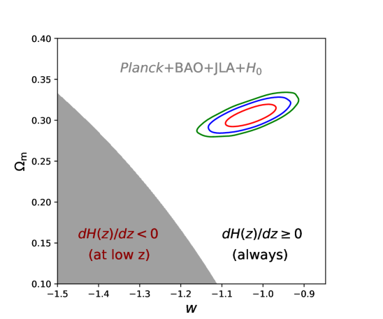
Figure 1: Consistency check of the monotonicity prior in the $w$CDM cosmology. The contours are joint constraints of Planck, BAO, JLA, and $H_{0}$ [43] and correspond to $68\%$, $95\%$, and $99\%$ confidence levels from inside out. The shaded area shows the sub-space rejected by the monotonicity prior.

In figure 1, we plot the marginalized constraints on $w$ and $\Omega_{\rm m}$ (the contours) from the combination of Planck, BAO, JLA, and $H_{0}$ [43] and show the $w$–$\Omega_{\rm m}$ sub-space that is rejected by the monotonicity prior (shaded area). As one sees from the figure, the combined observations rule out the possibility of an $E^{\prime}(z;\Omega_{\rm m},w)<0$ expansion history with a wide margin. Therefore, the monotonicity prior is reasonable within the $w$CDM model.

The EoS evolves with redshift in the $w_{a}$CDM model and is parameterized by $w(z)=w_{0}+w_{a}\frac{z}{1+z}$ [30, 31]. The expansion function is

$$E(z;\Omega_{\rm m},w_{0},w_{a})=\sqrt{\Omega_{\rm m}(1+z)^{3}+(1-\Omega_{\rm m})f_{X}(z)},$$ (2.12)

where

$$f_{X}(z)\equiv\exp\left[3\int_{0}^{z}\frac{1+w(z^{\prime})}{1+z^{\prime}}dz^{\prime}\right].$$ (2.13)

The derivative of the expansion function with respect to redshift is now given by

$$E^{\prime}(z;\Omega_{\rm m},w_{0},w_{a}) = \frac{3}{2}\frac{\Omega_{\rm m}(1+z)^{3}+(1-\Omega_{\rm m})[1+w(z)]f_{X}(z)}{(1+z)E(z;\Omega_{\rm m},w_{0},w_{a})}.$$ (2.14)

Figure 2 shows the marginalized constraints on $w_{0}$ and $w_{a}$ (contours) from the same set of data used in figure 1. Shaded areas in the left panel are the sub-space rejected by the monotonicity prior for different matter densities at $z=0.1$, and those in the right panel are the sub-space rejected by the monotonicity prior at different redshifts for $\Omega_{\rm m}=0.25$. As the matter density increases, the sub-space allowed by the monotonicity prior becomes larger and larger. From the right panel one finds that the sub-space allowed by the monotonicity prior increases with redshift for a fixed matter density. In all cases shown in figure 2, the monotonicity prior is consistent with existing observations under the $w_{a}$CDM model.

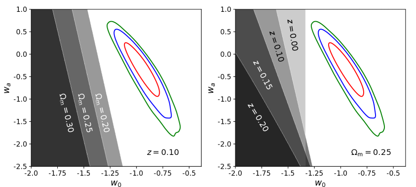
Figure 2: Same as figure 1 but for the $w_{a}$CDM cosmology. Shaded areas in the left panel represent the sub-space rejected by the monotonicity prior, at $z=0.1$ for different matter densities; those in the right panel represent the rejected sub-space at different redshifts for fixed matter density $\Omega_{\rm m}=0.25$.

Although we cannot enumerate all possible models, it is reasonable to take as a prior that the Hubble parameter increases monotonically with redshift.

2.3 Affine invariant MCMC ensemble sampling

We employ the affine invariant MCMC ensemble sampler proposed by Goodman $\&$ Weare [44] to explore the parameter space. This sampler’s algorithm has been demonstrated to be much more efficient than the traditional ones, e.g., the Metropolis-Hastings algorithm [45, 46, 47]. During the course of sampling, only one single position is updated in the Metropolis-Hastings algorithm, whereas an ensemble of $K$ walkers $W=\{X_{k}\}$ are evolved simultaneously in the affine invariant MCMC. The proposal distribution for the $k$-th walker is determined by the current positions of the other $K-1$ walkers in the complementary ensemble $W_{\left[k\right]}=\{X_{j},\forall j\neq k\}$, where the positions refer to vectors in the $N_{\rm p}$-dimensional parameter space. To update the position of a walker $X_{k}$, another walker $X_{j}$ is randomly drawn from the remaining walkers $W_{\left[k\right]}$ and a new position is proposed to be

$$X_{k}\rightarrow Y=X_{j}+R(X_{k}-X_{j}),$$ (2.15)

where $R$ is a random variable drawn from a distribution $g(r)$. The distribution $g(r)$ is required to have the following property

$$g(r^{-1})=r~{}g(r),$$ (2.16)

so that the proposal of eq. (2.15) is symmetric. An example for $g(r)$ is provided in [44, 46]

$$g(r)\propto\left\{\begin{array}[]{rr}\displaystyle\frac{1}{\sqrt{r}},&\mbox{if $r$ $\in\left[s^{-1},s\right]$},\\ 0,&\mbox{otherwise},\end{array}\right.$$ (2.19)

where $s$ is an adjustable scale parameter controlling the jumping step sizes of the walkers. The chains satisfies the condition of detailed balance if the proposed position $Y$ is accepted with the following probability

$$q=\min\left(1,R^{N_{\mathrm{p}}-1}\frac{p(Y)}{p(X_{k})}\right),$$ (2.20)

where $N_{\mathrm{p}}$ is the dimension of the parameter space. This procedure is then repeated for each of the rest walkers in the ensemble.

Two features of the affine invariant MCMC are worth attention. The first is that it is suitable for cases where parameters are strongly correlated with each other. Such correlations often cause high rejections of the proposed steps and thus lower the sampling efficiency of conventional algorithms. The affine invariant MCMC works well in these cases because of its affine-invariant property, and the sampling efficiency or acceptance ratio is controlled by a single parameter, the scale parameter $s$ in eq. (2.19). The second is that it can be naturally parallelized, which is crucial for computationally intensive problems, as shown by the pseudo-code in ref. [46].

We implement a C++ version of the sampler to reconstruct the Hubble parameter via MCMC. The chains produced by our sampler share the same format as that of CosmoMC, and they can be readily processed with the python package GetDist to get the best-fit values of the parameters and their corresponding confidence intervals.

3 Expansion history from SN Ia distances

In this section, we test the monotonicity prior using simulated SN Ia mock samples and reconstruct the cosmic expansion history from three existing SN Ia samples. We then apply the method to the expected WFIRST SN Ia sample and compare the resulting constraints on the cosmic expansion rate $E(z)$ with those from DESI BAO.

3.1 SN Ia samples

The SN Ia samples to be used for reconstruction include Union2.1 [32], SNLS3 [34, 33] and JLA [37, 36]. These compilations use the SALT2 model [48, 49] to fit the SNe Ia light-curves, from which the peak rest-frame B-band apparent magnitude $m_{\rm B}$ at the epoch of maximum light, the shape of the light-curve $S$ and the optical B-V color $C$ are measured. These quantities are then used to standardize the SN Ia peak luminosity. The measured distance modulus after correction can be written as a linear combination of the above measured quantities

$$\mu_{B}=m_{\rm B}-M_{\rm B}+\alpha\,S-\beta\,C,$$ (3.1)

where the B-band absolute magnitude $M_{\rm B}$ and the coefficients $\alpha$ and $\beta$ are fitted together with cosmological parameters. SNLS3 also uses SiFTO model [50] to fit the SNe Ia light-curves, but the shape parameter in eq. (3.1) is replaced by $s-1$. In table 1 we summarize the specific light-curve parameterizations adopted by these compilations: Union2.1 and JLA used exactly the same form as in eq. (3.1), whereas SNLS3 used the SiFTO parameterization; a detailed comparison of SLAT2 and SiFTO can be found in ref. [33], where transformations that relate the parameterizations of SiFTO and SLAT2 are also given.

Table 1: SN Ia Peak-light magnitude corrections.

SN Ia Compilation		Magnitude Correctionsa	Nuisance Parameters
Union2.1	$\mu_{\rm B}=$	$m_{\rm B}+\alpha\,x_{1}-\beta\,c+\delta\,P-M_{\rm B}$	$\alpha,\beta,M_{\rm B},\delta$
SNLS3	$m_{\rm B}=$	$5\log_{10}\mathcal{D}_{\rm L}-\alpha(s-1)+\beta\,C+\mathcal{M}_{\rm B}$	$\alpha,\beta,\mathcal{M}_{\rm B}$ (or $\mathcal{M}^{1}_{\rm B},\mathcal{M}^{2}_{\rm B}$)
JLA	$\mu_{\rm B}=$	$m_{\rm B}-(M_{\rm B}-\alpha\,X_{1}+\beta\,C)$	$\alpha,\beta,M_{\rm B}$ (or $M_{\rm B}^{1},\Delta_{\rm M}$)

• These expressions have been simplified for clarity.

The SN Ia luminosity slightly correlates with the host galaxy mass [51]. This correlation is accounted for by introducing new parameters to the peak-light magnitude corrections, as shown in table 1. Union2.1 models this correlation with the term $\delta\,P$, where $\delta$ is the host-mass-correction coefficient and $P$ is the probability for a SN Ia to have a host galaxy less massive than $10^{10}m_{\odot}$. SNLS3 and JLA divide their SNe Ia into two sub-samples, one for SNe Ia with host galaxies less massive than $10^{10}m_{\odot}$ and the other for those with more massive hosts. SNLS3 assigns two reduced peak absolute magnitudes, $\mathcal{M}_{\rm B}^{1}$ and $\mathcal{M}_{\rm B}^{2}$, to its two sub-samples, respectively; JLA uses a single peak absolute magnitude parameter $M_{\rm B}^{1}$ for all SNe Ia, and adds an offset $\Delta_{\rm M}$ to $M_{\rm B}^{1}$ for those SNe Ia in more massive host galaxies.

There are many systematics that affect the constraints on cosmological parameters. The zero-point uncertainties and the absolute magnitude calibration are the dominant effects. Others include Malmquist bias, galactic and intergalactic extinction, rest-frame U-band calibration, non-SN Ia contamination as well as gravitational lensing [12, 32, 34, 33, 37, 36]. All the three compilations propagate these systematics into the total covariance matrices. SNLS3 and JLA further take into account the systematics induced by peculiar velocities and possible evolution of SN Ia.

The total covariance matrix can be decomposed into a summation of three terms following the convention in ref. [33]:

$$\mathbf{C}=\mathbf{D}_{\rm{stat}}+\mathbf{C}_{\rm{stat}}+\mathbf{C}_{\rm{sys}}.$$ (3.2)

The off-diagonal parts $\mathbf{C}_{\rm{stat}}$ and $\mathbf{C}_{\rm{sys}}$ are the statistical and systematical correlations between different SNe Ia, and they can be computed using the standard techniques described in ref. [52]. The diagonal matrix $\mathbf{D}_{\rm{stat}}$ represents statistical uncertainties of the SNe Ia

$$\mathbf{D}_{{\rm{stat}},ii} = \sigma^{2}_{m_{\rm B},i}+\alpha^{2}\sigma_{s,i}^{2}+\beta^{2}\sigma_{C,i}^{2}+\sigma^{2}_{\rm{int}}+\left(\frac{5(1+z_{i})}{z_{i}(1+z_{i}/2)\log{10}}\right)^{2}\sigma^{2}_{z,i}$$ (3.3)

$$+ \sigma^{2}_{\rm{lens}}+\sigma^{2}_{\rm{host}}+{\mathbf{C}}_{m_{B}\,s\,C,i},$$

where $\sigma^{2}_{m_{\rm B},i}$, $\sigma_{s,i}^{2}$ and $\sigma_{C,i}^{2}$ are the variances of the measured light-curve parameters, $\sigma^{2}_{\rm{int}}$ accounts for the intrinsic scatter of SN Ia, the term proportional to $\sigma^{2}_{z,i}$ is the magnitude variance associated with redshift uncertainty (with $z_{i}$ being the redshift of the $i$th SN Ia in the CMB rest frame), $\sigma^{2}_{\rm{lens}}$ is caused by gravitational lensing, $\sigma^{2}_{\rm{host}}$ comes from the correlation of SN Ia luminosity to the stellar mass of its host galaxy, the last term ${\mathbf{C}}_{m_{B}\,s\,C,i}$ represents three covariances between the light-curve parameters as well as the apparent magnitude for each SN Ia and is a function of $\alpha$ and $\beta$. The (total) statistical uncertainties depend on the light-curve parameters $\alpha$ and $\beta$, which can not be analytically marginalized and are fitted together with the cosmological parameters (the strategy used in SNLS3 and JLA); Union2.1 provides total covariance matrices with and without systematics, in which $\alpha$ and $\beta$ (as well as $\delta$) assume their best-fit values.

The intrinsic scatter term $\sigma_{\rm{int}}$ is sourced from two parts. One is the true dispersion in the peak absolute luminosity reflecting the imperfection of these standardized candles, and the other includes systematics that are currently unknown. Unfortunately, these two parts can not be distinguished from each other. To obtain an estimate of $\sigma_{\rm{int}}$, one usual method is to fit the data to a fiducial model (the flat $w$CDM model is often adopted) and adjust $\sigma^{2}_{\rm{int}}$ until the best-fit $\chi^{2}$ to be one per degree of freedom. However, this procedure precludes the statistical tests of the adequacy of the cosmological model to describe the data [34, 37]. The unknown systematics are generally sample-dependent, and SNLS3 and JLA compilations have estimated $\sigma_{\rm{int}}$ for each of their sub-samples (see table 2). Although Union2.1 has estimated $\sigma_{\rm{int}}$ for its 19 sub-samples, only the median value $\sigma_{\rm{int}}^{\rm median}=0.15$ is used to construct the covariance matrix [32].

Table 2: Intrinsic scatter $\sigma_{\rm{int}}$ of the sub-samples in SNLS3 [34] and JLA [37].

Sub-sample	SNLS3	JLA
Low-z	0.113	0.134
SDSS	0.099	0.108
SNLS	0.068	0.080
HST	0.082	0.100

3.2 Tests with mock samples

We construct two mock SN Ia samples to test the reconstruction method. The first one is generated from the real JLA SN Ia sample, sharing exactly the same redshifts as those of JLA [37, 36] (hereafter JLA-mock). To simulate random magnitude errors, a full covariance matrix for all the 740 SNe Ia is constructed from the covariance matrices provided by the JLA compilation, with the light-curve nuisance parameters $\alpha$ and $\beta$ fixed to 0.13 and 3.1, respectively. The errors are then randomly drawn from the multivariate Gaussian distribution (with zero means) specified by the total covariance matrix, which is also used in the JLA-mock likelihood calculations.

The second one assumes the redshift distribution expected from WFIRST [53], which will be able to measure over 2700 SNe Ia in the redshift range $0.1\leq z\leq 1.7$ (hereafter WFIRST-mock). The magnitude errors are randomly drawn from the WFIRST Gaussian error model [53]

$$\sigma_{\mu}^{2}(z)=\sigma^{2}_{\rm{int}}+\sigma^{2}_{\rm{meas}}+\sigma^{2}_{\rm{lens}}+\sigma^{2}_{\rm{sys}},$$ (3.4)

where $\sigma_{\rm{int}}=0.09$ is the intrinsic spread of the SN Ia peak absolute magnitude (after correcting for the light-curve shape and spectral properties), $\sigma_{\rm{meas}}=0.08$ is the photometry error, $\sigma_{\rm{lens}}=0.07z$ accounts for lensing magnification, and $\sigma_{\rm{sys}}=0.02(1+z)/1.8$ is the assumed systematics. The magnitude errors of different SNe Ia in this mock are assumed to be uncorrelated for simplicity.

The two mock SN Ia samples are generated assuming a flat $\Lambda$CDM cosmology with the following fiducial parameters: $H_{0}=70.0~{}\rm{km~{}s^{-1}~{}Mpc^{-1}}$, $\Omega_{\rm m}=0.3$, and $\Omega_{\Lambda}=0.7$. The fiducial value of the SN Ia peak absolute magnitude is assumed to be $M_{\rm B}=-19.3$. In the following tests, the reduced peak absolute magnitude is fitted together with the cosmic expansion rate $\{E_{i}\}$ and then marginalized.

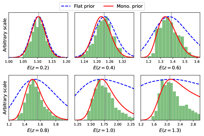
Figure 3: Marginalized posterior distributions of the cosmic expansion rate $\{E_{i}\}$ at different redshifts from the JLA-mock (curves) and distributions of the maximum-likelihood $\{E_{i}\}$ values from 1000 random realizations of mock JLA data with the monotonicity prior (histograms). The solid and dashed curves are the results reconstructed with and without the monotonicity prior, respectively. The results are all normalized to the same peak height. The vertical lines indicate the input values.

The marginalized posterior distributions of the cosmic expansion rate $\{E_{i}\}$ reconstructed from the JLA-mock is shown in figure 3. The reconstructed results recover the input values (vertical lines) fairly well, and the reconstruction uncertainties are reduced considerably by the monotonicity prior (solid curves) at $z\gtrsim 0.6$. Since the distance modulus $\mu(z)$ involves an integration over $\hat{E}^{-1}(z)$ from $0$ to $z$, the cosmic expansion rate at the first few interpolation nodes are constrained by not only the low redshift SNe Ia but also those at higher redshifts. Therefore the cosmic expansion rate at low redshifts can still be well constrained even without the monotonicity prior.

Although the results of the particular mock data do not appear to be biased, the ensemble behavior of the estimator can differ (e.g., [54]). Biases may be present in the distributions of values estimated from an ensemble of realizations. One can determine an optimal balance between the ensemble bias and the ensemble variance with a large number of random mocks (e.g., [27]). For the purpose of this work, we simply draw 1000 realizations of mock JLA data and examine the probability distributions of the maximum-likelihood values of the expansion rate obtained with the monotonicity prior. The resulting histograms in figure 3 are skewed in some cases, but the biases are small compared to the posterior distributions from the single JLA-mock, which characterize parameter uncertainties in the usual MCMC analysis.

Figure 4 shows the expansion rate $\{E_{i}\}$ reconstructed from the WFIRST-mock. One sees the same improvements as those in figure 3. Since the WFIRST-mock contains about 300 SNe Ia in the range $1.4<z\leq 1.7$, a lot more than those in the JLA-mock, the expansion rate at the last interpolation node, $E(z=1.7)$, can still be constrained fairly well. At low redshift, however, the JLA-mock has many more SNe Ia than the WFIRST-mock and hence provides a tighter constraint at $z=0.2$. Similar to the case of JLA, the distributions of the estimated $\{E_{i}\}$ values from 1000 realizations of mock WFIRST data are not biased appreciably.

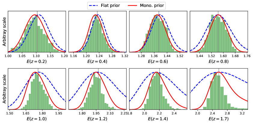
Figure 4: Same as figure 3 but for the WFIRST-mock. Since the WFIRST-mock extends to redshift $z=1.7$, two more interpolation nodes are added.

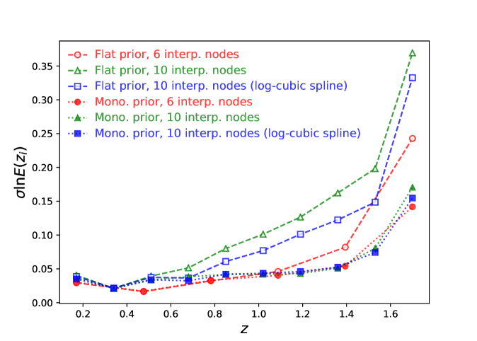
Figure 5: Fractional errors of the cosmic expansion rate $\{E_{i}\}$ reconstructed from the WFIRST-mock: circles for 6-node log-linear interpolation, triangles for 10-node log-linear interpolation, and squares for 10-node log-cubic spline interpolation. Open symbols represent results with the flat prior, and solid symbols represent those with the monotonicity prior.

Figure 5 compares the fractional errors on the cosmic expansion rate reconstructed from the WFIRST-mock with 6-node (circles) and 10-node (triangles) log-linear interpolations as defined by eq. 2.1. In addition, we also include the results of 10-node log-cubic spline interpolation (squares) to check the effect of the interpolation scheme on the reconstruction.

When the flat prior is applied (open symbols), the fractional errors at redshifts $z\gtrsim 0.7$ increase quickly with the number of interpolation nodes. The interpolated deceleration and jerk functions are continuous with the log-cubic spline interpolation, which is effectively an additional constraint on the expansion rate. Therefore, the 10-node log-cubic spline interpolation achieves smaller uncertainties of $\{E_{i}\}$ than the 10-node log-linear interpolation does. When the monotonicity prior is enforced (solid symbols), the fractional errors are significantly reduced and remain less than $5\%$ up to redshift $z\simeq 1.4$. It is somewhat surprising that the errors are fairly independent of the number of interpolation nodes and interpolation schemes. Because the added interpolation nodes limit the allowable variation of the Hubble parameter at each redshift, the strength of the monotonicity prior actually increases with the number of interpolation nodes assigned to the same redshift range, largely canceling the effect of increasing number of interpolation nodes.

3.3 Expansion history from existing SN Ia samples

Table 3: Cosmic expansion rate and Hubble parameter (${\rm km~{}s^{-1}Mpc^{-1}}$) reconstructed from Union2.1, SNLS3 and JLA.

$z_{i}$	Union2.1a		SNLS3a		JLAa
	$E(z_{i})$	$H(z_{i})$	$E(z_{i})$	$H(z_{i})$	$E(z_{i})$	$H(z_{i})$
0.2	$1.09_{-0.03}^{+0.04}$	$79.5_{-2.9}^{+3.3}$	$1.08_{-0.03}^{+0.03}$	$79.0_{-2.5}^{+2.7}$	$1.11_{-0.03}^{+0.02}$	$81.5_{-2.6}^{+2.5}$
0.4	$1.21_{-0.06}^{+0.06}$	$88.8_{-4.3}^{+4.9}$	$1.12_{-0.03}^{+0.04}$	$82.2_{-3.3}^{+3.5}$	$1.22_{-0.04}^{+0.04}$	$89.1_{-3.5}^{+3.7}$
0.6	$1.35_{-0.07}^{+0.09}$	$99.1_{-5.7}^{+6.5}$	$1.19_{-0.06}^{+0.07}$	$87.1_{-4.8}^{+5.9}$	$1.34_{-0.06}^{+0.08}$	$98.1_{-5.0}^{+6.2}$
0.8	$1.48_{-0.10}^{+0.12}$	$109_{-7.0}^{+9.0}$	$1.35_{-0.10}^{+0.13}$	$99.0_{-8.0}^{+10}$	$1.43_{-0.08}^{+0.09}$	$105_{-6.0}^{+7.0}$
1.0	$1.66_{-0.15}^{+0.23}$	$122_{-12}^{+17}$	$1.56_{-0.17}^{+0.27}$	$115_{-13}^{+20}$	$1.57_{-0.13}^{+0.21}$	$115_{-10}^{+16}$

• The results are obtained with the monotonicity prior. The quoted values correspond to the peak positions of the marginalized one-dimensional distributions and $68\%$ confidence levels.

Table 3 summarizes the cosmic expansion rate $\{E_{i}\}$ and the Hubble parameter $\{H_{i}\}$ reconstructed from the three SN Ia compilations. The values of $\{H_{i}\}$ are mapped from $\{E_{i}\}$ using the prior $H_{0}=73.24\pm 1.74~{}\rm{km~{}s^{-1}~{}Mpc^{-1}}$, which is based on the combination of maser distance of NGC 4258, trigonometric parallaxes of Milky Way Cepheids and Cepheids in the Large Magellanic Cloud [42, Riess16]. Results at the last interpolation node of each compilation are rather poor (see e.g., figure 6), so they are not included in table 3. The results from Union2.1 and JLA are consistent with each other, whereas the SNLS3 results at $z=0.4$ and $0.6$ are considerably lower than those from the other two datasets. Reconciling the differences is beyond the scope of this work. Nevertheless, we note that inconsistency also exists between the inferred matter density $\Omega_{\rm m}$ from SNLS3 and those from Union2.1 and JLA, which has been attributed to an unanticipated systematic effect [37].

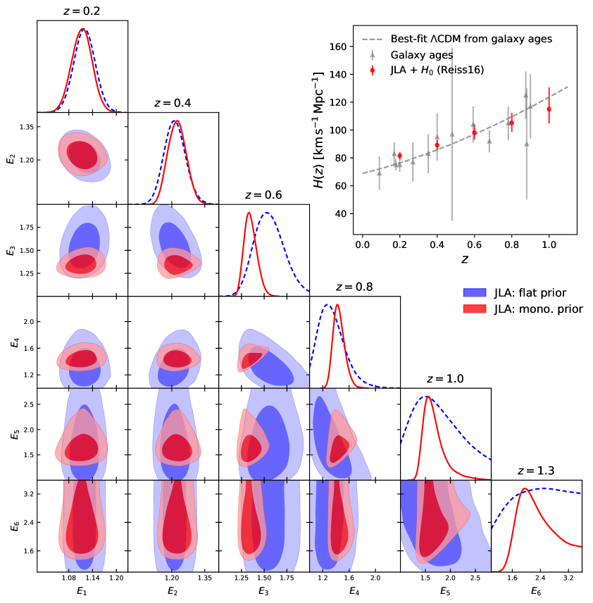
Figure 6: Constraints on the cosmic expansion rate $\{E_{i}\}$ from JLA. The marginalized one dimensional probability density distributions in the panels along the diagonal are normalized to the same peak height. The inset shows the Hubble parameter $\{H_{i}\}$ (circles), which is mapped from JLA-reconstructed $\{E_{i}\}$ and the Reiss16 $H_{0}$ measurement, along with those derived from galaxy age data (triangles) [20, 21] and the best-fit $\Lambda$CDM $H(z)$ (dashed line) of the galaxy age data.

Figure 6 presents the cosmic expansion rate $\{E_{i}\}$ reconstructed from the JLA sample. The marginalized probability density distributions of $\{E_{i}\}$, obtained with and without the monotonicity prior (solid curves and dashed curves, respectively), are compared in the panels along the diagonal, showing similar improvements brought by the monotonicity prior as seen in figure 3. The inset in figure 6 shows the Hubble parameter $\{H_{i}\}$ (circles) mapped from $\{E_{i}\}$ and those derived from the ages of passively evolving galaxies (triangles) [20, 21]. The JLA-reconstructed $\{H_{i}\}$ is consistent with the predicted $H(z)$ (dashed line) in the best-fit $\Lambda$CDM model of the galaxy age data, which has best-fit $H_{0}=68.86~{}\rm{km~{}s^{-1}~{}Mpc^{-1}}$ and $\Omega_{\rm m}=0.317$. Figure 6 and table 3 demonstrate that, with the help of the monotonicity prior, existing SN Ia samples already provide fairly well and model independent constraints on the cosmic expansion history at $z\lesssim 1$.

3.4 Forecast for WFIRST

Here we give a comparison of the constraints on the expansion history expected from DESI and WFIRST. DESI will measure $\{H_{i}\}$ from the radial BAO signal. We adopt the results from Table V of ref. [55], which covers $z=0.15$ to 1.85 in intervals of $\Delta z=0.1$. WFIRST has a spectroscopic BAO survey component, but we only use its SN Ia results on $\{E_{i}\}$ described in section 3.2.

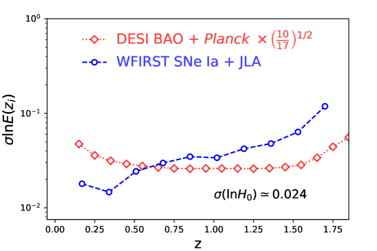
Figure 7: Fractional errors of $\{E_{i}\}$ expected from DESI BAO (diamonds, with Planck) and WFIRST SNe Ia (circles, with JLA). The DESI errors have been rescaled for a proper comparison.

To compare the results, we convert the uncertainties of $\{H_{i}\}$ from DESI to those of $\{E_{i}\}$ with an independent prior $\sigma\left(\ln H_{0}\right)\simeq 0.024$ [42], using the following relation

$$\sigma^{2}(\ln E_{i}) = \sigma^{2}(\ln H_{i})+\sigma^{2}(\ln H_{0}).$$ (3.5)

Moreover, we normalize the errors on $\{\ln H_{i}\}$ by the square root of the number of constraints within the same redshift range to compare the results of different datasets on a roughly equal footing [29]. The multiplicative factor for DESI is $\left(\frac{10}{17}\right)^{1/2}$, where the numerator in the parenthesis is the number of interpolation nodes for WFIRST SNe Ia within $0.1<z\leq 1.7$ and the denominator is the number of DESI constraints within roughly the same redshift range.

Figure 7 shows the expected fractional errors on the expansion rate from WFIRST SNe Ia and DESI BAO. The DESI results include the CMB prior from Planck. The WFIRST-mock results are obtained with the monotonicity prior enforced, and the JLA-mock is added to strengthen the constraints at the lowest redshifts. In terms of $\{E_{i}\}$, WFIRST SNe Ia can achieve a few percent level constraints at redshift lower than $z\simeq 1$, fairly competitive to DESI BAO, though the conclusion depends on the assumed uncertainty of the $H_{0}$ measurement. At higher redshift, the SN Ia data degrades quickly and become less competitive than DESI BAO.

4 Summary

In this work we propose a monotonicity prior for non-parametric reconstruction of the cosmic expansion history, which requires the Hubble parameter $H(z)$ or the expansion rate $E(z)$ to always increase with redshift. This prior is reasonably well motivated, even though no theory so far prohibits a reverse of the trend at some point in the past. Using SN Ia luminosity distances as an example, we demonstrate that the monotonicity prior is highly effective in reducing errors on the reconstructed $\{E_{i}\}$ and that it does not introduce appreciable biases. The improvement is most significant at high redshift where the SN Ia data is poor. It is also helpful that the monotonicity prior keeps the uncertainties of the reconstructed $\{E_{i}\}$ fairly independent of the number of interpolation nodes assigned for the SN Ia data.

Application of the monotonicity prior to existing SN Ia compilations is able to constrain $\{E_{i}\}$ to 3%–6% at four redshifts up to $z=0.8$ and 14% at $z=1$. When converted to the Hubble parameter using the prior of $H_{0}=73.24\pm 1.74~{}\rm{km~{}s^{-1}~{}Mpc^{-1}}$, the results are consistent with those derived from galaxy ages. Future SN Ia sample from WFIRST can achieve $\lesssim 5\%$ errors on $\{E_{i}\}$ at redshifts up to $z\sim 1.4$, which is competitive with DESI BAO at low redshift. Given that WFIRST SNe Ia and DESI BAO are highly independent of each other, their combination will tightly constrain $\{E_{i}\}$ across the entire redshift range of the data. Moreover, SNe Ia data is sensitive to the expansion rate, while BAO and WL are sensitive to the Hubble parameter. Hence, the combination of these probes can determine the Hubble constant as well.

We note that the expansion history reconstructed from SN Ia distances dose not provide more information than the distances themselves do, but it offers a convenient way to compare the results of different methods. The monotonicity prior is helpful for the reconstruction from SN Ia data and should be also applicable to other probes such as BAOs that measure the Hubble parameter at multiple redshifts. Even if the expansion history is not directly reconstructed, one may still enforce the monotonicity prior by requiring the Hubble parameter or the expansion rate to increase with redshift monotonically in the MCMC-sampled cosmological models. Better cosmological constraints could be achieved in this way. Moreover, we expect that the monotonicity prior can be generalized to other cosmological quantities that are reasonably monotonic with redshift.

Appendix A An efficient implementation of the monotonicity prior

The monotonicity prior on the cosmic expansion history rules out most part of the parameter space spanned by $\{E_{i}\}$. However, the MCMC sampler is unaware of this exclusion zone a priori and has to test it on the fly. The MCMC sampling is therefore rather inefficient in $\{E_{i}\}$ parametrization, especially when its dimension becomes large. The sampling efficiency can be greatly improved by a change of parameters as follows. Let the new set of parameters $\bm{\eta}\equiv\{\eta_{i}\}$ be defined through

$$E_{i}-1=\prod_{n=i}^{N}\eta_{n},$$ (A.1)

where $N$ is the number of interpolation nodes, $0<\eta_{i}\leq 1$ for $1\leq i\leq N-1$, and $\eta_{N}=E_{N}-1$. Because eq. (A.1) preserves the relation $E_{i}\leq E_{i+1}$, sampling in $\bm{\eta}$ space satisfies the monotonicity prior automatically and is thus far more efficient than that in $\bm{E}$ space. The probability $\pi(\bm{\eta})$ is given by

$$\pi(\bm{\eta})=\left|\frac{\partial\bm{E}}{\partial\bm{\eta}}\right|\pi(\bm{E})=\prod_{i=2}^{N}\eta_{i}^{i-1},$$ (A.2)

where we have made use of $\pi(\bm{E})=1$. After a sample of $\bm{\eta}$ is obtained, one can map it into a sample of $\bm{E}$ using eq. (A.1).

References

- [1] A. G. Riess, A. V. Filippenko, P. Challis, A. Clocchiatti, A. Diercks, P. M. Garnavich et al., Observational Evidence from Supernovae for an Accelerating Universe and a Cosmological Constant, Astron. J. 116 (Sept., 1998) 1009–1038, [astro-ph/9805201].
- [2] S. Perlmutter, G. Aldering, G. Goldhaber, R. A. Knop, P. Nugent, P. G. Castro et al., Measurements of and from 42 High-Redshift Supernovae, Astrophys. J. 517 (June, 1999) 565–586, [astro-ph/9812133].
- [3] I. Zlatev, L. Wang and P. J. Steinhardt, Quintessence, Cosmic Coincidence, and the Cosmological Constant, Physical Review Letters 82 (Feb., 1999) 896–899, [astro-ph/9807002].
- [4] P. J. Steinhardt, L. Wang and I. Zlatev, Cosmological tracking solutions, Phys. Rev. D 59 (June, 1999) 123504, [astro-ph/9812313].
- [5] De Felice, Antonio and Tsujikawa, Shinji, theories, Living Reviews in Relativity 13 (2010) 3.
- [6] S. Tsujikawa, Quintessence: a review, Classical and Quantum Gravity 30 (Nov., 2013) 214003, [1304.1961].
- [7] P. Singh, M. Sami and N. Dadhich, Cosmological dynamics of a phantom field, Phys. Rev. D 68 (July, 2003) 023522, [hep-th/0305110].
- [8] A. Kamenshchik, U. Moschella and V. Pasquier, An alternative to quintessence, Physics Letters B 511 (July, 2001) 265–268, [gr-qc/0103004].
- [9] V. Gorini, A. Kamenshchik, U. Moschella and V. Pasquier, The Chaplygin Gas as a Model for Dark Energy, in The Tenth Marcel Grossmann Meeting. On recent developments in theoretical and experimental general relativity, gravitation and relativistic field theories (M. Novello, S. Perez Bergliaffa and R. Ruffini, eds.), p. 840, Feb., 2006, gr-qc/0403062, DOI.
- [10] M. C. Bento, O. Bertolami and A. A. Sen, Generalized Chaplygin gas, accelerated expansion, and dark-energy-matter unification, Phys. Rev. D 66 (Aug., 2002) 043507, [gr-qc/0202064].
- [11] T. P. Sotiriou and V. Faraoni, theories of gravity, Reviews of Modern Physics 82 (Jan., 2010) 451–497, [0805.1726].
- [12] R. Amanullah, C. Lidman, D. Rubin, G. Aldering, P. Astier, K. Barbary et al., Spectra and Hubble Space Telescope Light Curves of Six Type Ia Supernovae at 0.511 z 1.12 and the Union2 Compilation, Astrophys. J. 716 (June, 2010) 712–738, [1004.1711].
- [13] G. Dvali, G. Gabadadze and M. Porrati, 4D gravity on a brane in 5D Minkowski space, Physics Letters B 485 (July, 2000) 208–214, [hep-th/0005016].
- [14] Y. Wang, Differentiating dark energy and modified gravity with galaxy redshift surveys, J. Cosmo. Astropart. Phys. 5 (May, 2008) 021, [0710.3885].
- [15] A. Shafieloo, A. G. Kim and E. V. Linder, Model independent tests of cosmic growth versus expansion, Phys. Rev. D 87 (Jan., 2013) 023520, [1211.6128].
- [16] D. Huterer and et al., Growth of cosmic structure: Probing dark energy beyond expansion, Astroparticle Physics 63 (Mar., 2015) 23–41, [1309.5385].
- [17] H.-J. Seo and D. J. Eisenstein, Probing Dark Energy with Baryonic Acoustic Oscillations from Future Large Galaxy Redshift Surveys, Astrophys. J. 598 (Dec., 2003) 720–740, [astro-ph/0307460].
- [18] W. Hu and Z. Haiman, Redshifting rings of power, Phys. Rev. D 68 (Sept., 2003) 063004, [astro-ph/0306053].
- [19] D. J. Eisenstein, I. Zehavi, D. W. Hogg, R. Scoccimarro, M. R. Blanton, R. C. Nichol et al., Detection of the Baryon Acoustic Peak in the Large-Scale Correlation Function of SDSS Luminous Red Galaxies, Astrophys. J. 633 (Nov., 2005) 560–574, [astro-ph/0501171].
- [20] R. Jimenez and A. Loeb, Constraining Cosmological Parameters Based on Relative Galaxy Ages, Astrophys. J. 573 (July, 2002) 37–42, [astro-ph/0106145].
- [21] S. M. Crawford, A. L. Ratsimbazafy, C. M. Cress, E. A. Olivier, S.-L. Blyth and K. J. van der Heyden, Luminous red galaxies in simulations: cosmic chronometers?, Mon. Not. Roy. Astron. Soc. 406 (Aug., 2010) 2569–2577, [1004.2378].
- [22] Y. Wang and M. Tegmark, Uncorrelated measurements of the cosmic expansion history and dark energy from supernovae, Phys. Rev. D 71 (May, 2005) 103513, [astro-ph/0501351].
- [23] A. Sandage, The Change of Redshift and Apparent Luminosity of Galaxies due to the Deceleration of Selected Expanding Universes., Astrophys. J. 136 (Sept., 1962) 319.
- [24] A. Loeb, Direct Measurement of Cosmological Parameters from the Cosmic Deceleration of Extragalactic Objects, Astrophys. J. Lett. 499 (June, 1998) L111–L114, [astro-ph/9802122].
- [25] H. Zhan, Rees-Sciama Effect and Impact of Foreground Structures on Galaxy Redshifts, Astrophys. J. 740 (Oct., 2011) 26, [1105.5249].
- [26] V. Sahni and A. Starobinsky, Reconstructing Dark Energy, International Journal of Modern Physics D 15 (2006) 2105–2132, [astro-ph/0610026].
- [27] S. D. P. Vitenti and M. Penna-Lima, A general reconstruction of the recent expansion history of the universe, J. Cosmo. Astropart. Phys. 9 (Sept., 2015) 045, [1505.01883].
- [28] D. Huterer and G. Starkman, Parametrization of Dark-Energy Properties: A Principal-Component Approach, Physical Review Letters 90 (Jan., 2003) 031301, [astro-ph/0207517].
- [29] H. Zhan, L. Knox and J. A. Tyson, Distance, Growth Factor, and Dark Energy Constraints from Photometric Baryon Acoustic Oscillation and Weak Lensing Measurements, Astrophys. J. 690 (Jan., 2009) 923–936, [0806.0937].
- [30] M. Chevallier and D. Polarski, Accelerating Universes with Scaling Dark Matter, International Journal of Modern Physics D 10 (2001) 213–223, [gr-qc/0009008].
- [31] E. V. Linder, Exploring the Expansion History of the Universe, Physical Review Letters 90 (Mar., 2003) 091301, [astro-ph/0208512].
- [32] N. Suzuki, et al. and Supernova Cosmology Project, The Hubble Space Telescope Cluster Supernova Survey. V. Improving the Dark-energy Constraints above and Building an Early-type-hosted Supernova Sample, Astrophys. J. 746 (Feb., 2012) 85, [1105.3470].
- [33] J. Guy, M. Sullivan, A. Conley, N. Regnault, P. Astier, C. Balland et al., The Supernova Legacy Survey 3-year sample: Type Ia supernovae photometric distances and cosmological constraints, Astron. & Astrophys. 523 (Nov., 2010) A7, [1010.4743].
- [34] A. Conley, J. Guy, M. Sullivan, N. Regnault, P. Astier, C. Balland et al., Supernova Constraints and Systematic Uncertainties from the First Three Years of the Supernova Legacy Survey, Astrophys. J. Supp. 192 (Jan., 2011) 1, [1104.1443].
- [35] M. Sullivan, J. Guy, A. Conley, N. Regnault, P. Astier, C. Balland et al., SNLS3: Constraints on Dark Energy Combining the Supernova Legacy Survey Three-year Data with Other Probes, Astrophys. J. 737 (Aug., 2011) 102, [1104.1444].
- [36] M. Betoule, J. Marriner, N. Regnault, J.-C. Cuillandre, P. Astier, J. Guy et al., Improved photometric calibration of the SNLS and the SDSS supernova surveys, Astron. & Astrophys. 552 (Apr., 2013) A124, [1212.4864].
- [37] M. Betoule, R. Kessler, J. Guy, J. Mosher, D. Hardin, R. Biswas et al., Improved cosmological constraints from a joint analysis of the SDSS-II and SNLS supernova samples, Astron. & Astrophys. 568 (Aug., 2014) A22, [1401.4064].
- [38] P. Mukherjee, D. Parkinson and A. R. Liddle, A nested sampling algorithm for cosmological model selection, The Astrophysical Journal Letters 638 (2006) L51.
- [39] R. Trotta, Applications of Bayesian model selection to cosmological parameters, Mon. Not. Roy. Astron. Soc. 378 (June, 2007) 72–82, [astro-ph/0504022].
- [40] M. P. Lima, S. Vitenti and M. J. Rebouças, Energy condition bounds and their confrontation with supernovae data, Phys. Rev. D 77 (Apr., 2008) 083518, [0802.0706].
- [41] Y. L. Bolotin, V. A. Cherkaskiy, O. A. Lemets, D. A. Yerokhin and L. G. Zazunov, Cosmology In Terms Of The Deceleration Parameter. Part I, ArXiv e-prints (Feb., 2015) , [1502.00811].
- [42] A. G. Riess, L. M. Macri, S. L. Hoffmann, D. Scolnic, S. Casertano, A. V. Filippenko et al., A determination of the local value of the hubble constant, The Astrophysical Journal 826 (2016) 56.
- [43] Planck Collaboration, P. A. R. Ade, N. Aghanim, M. Arnaud, M. Ashdown, J. Aumont et al., Planck 2015 results. XIII. Cosmological parameters, Astron. & Astrophys. 594 (Sept., 2016) A13, [1502.01589].
- [44] Jonathan Goodman and Jonathan Weare, Ensemble samplers with affine invariance, Communications in Applied Mathematics and Computational Science 5 (2010) .
- [45] F. Hou, J. Goodman, D. W. Hogg, J. Weare and C. Schwab, An Affine-invariant Sampler for Exoplanet Fitting and Discovery in Radial Velocity Data, Astrophys. J. 745 (Feb., 2012) 198, [1104.2612].
- [46] D. Foreman-Mackey, D. W. Hogg, D. Lang and J. Goodman, emcee: The MCMC Hammer, Pub. Astron. Soc. Pacific 125 (Mar., 2013) 306, [1202.3665].
- [47] J. Akeret, S. Seehars, A. Amara, A. Refregier and A. Csillaghy, CosmoHammer: Cosmological parameter estimation with the MCMC Hammer, Astronomy and Computing 2 (Aug., 2013) 27–39.
- [48] J. Guy, P. Astier, S. Nobili, N. Regnault and R. Pain, SALT: a spectral adaptive light curve template for type Ia supernovae, Astron. & Astrophys. 443 (Dec., 2005) 781–791, [astro-ph/0506583].
- [49] J. Guy, P. Astier, S. Baumont, D. Hardin, R. Pain, N. Regnault et al., SALT2: using distant supernovae to improve the use of type Ia supernovae as distance indicators, Astron. & Astrophys. 466 (Apr., 2007) 11–21, [astro-ph/0701828].
- [50] A. Conley and M. Sullivan, ‘SiFTO: An Empirical Method for Fitting SN Ia Light Curves.’ Astrophysics Source Code Library, Oct., 2011. doi:10.20356/C4K01V.
- [51] M. Sullivan, A. Conley, D. A. Howell, J. D. Neill, P. Astier, C. Balland et al., The dependence of Type Ia Supernovae luminosities on their host galaxies, Mon. Not. Roy. Astron. Soc. 406 (Aug., 2010) 782–802, [1003.5119].
- [52] B. Aharmim and et al., Electron energy spectra, fluxes, and day-night asymmetries of 8B solar neutrinos from measurements with NaCl dissolved in the heavy-water detector at the Sudbury Neutrino Observatory, Phys. Rev. C 72 (Nov., 2005) 055502, [nucl-ex/0502021].
- [53] D. Spergel, N. Gehrels, C. Baltay, D. Bennett, J. Breckinridge, M. Donahue et al., Wide-Field InfrarRed Survey Telescope-Astrophysics Focused Telescope Assets WFIRST-AFTA 2015 Report, ArXiv e-prints (Mar., 2015) , [1503.03757].
- [54] L. Sun, Q. Wang and H. Zhan, Likelihood of the Power Spectrum in Cosmological Parameter Estimation, Astrophys. J. 777 (Nov., 2013) 75, [1306.5064].
- [55] A. Font-Ribera, P. McDonald, N. Mostek, B. A. Reid, H.-J. Seo and A. Slosar, DESI and other Dark Energy experiments in the era of neutrino mass measurements, J. Cosmo. Astropart. Phys. 5 (May, 2014) 023, [1308.4164].