Arbitrary beam control using passive lossless metasurfaces enabled by orthogonally-polarized custom surface waves

Abstract

For passive, lossless impenetrable metasurfaces, a design technique for arbitrary beam control of receiving, guiding, and launching is presented. Arbitrary control is enabled by a custom surface wave in an orthogonal polarization such that its addition to the incident (input) and the desired scattered (output) fields is supported by a reactive surface impedance everywhere on the reflecting surface. Such a custom surface wave (SW) takes the form of an evanescent wave propagating along the surface with a spatially varying envelope. A growing SW appears when an illuminating beam is received. The SW amplitude stays constant when power is guided along the surface. The amplitude diminishes as a propagating wave (PW) is launched from the surface as a leaky wave. The resulting reactive tensor impedance profile may be realized as an array of anisotropic metallic resonators printed on a grounded dielectric substrate. Illustrative design examples of a Gaussian beam translator-reflector, a probe-fed beam launcher, and a near-field focusing lens are provided.

I Introduction

Comprising an electrically thin layer of subwavelength resonators Holloway et al. (2012), metasurfaces are capable of tailoring the characteristics of propagating and evanescent waves with a significantly reduced loss compared with traditional volumetric metamaterials. In particular, gradient metasurfaces, those with spatially varying surface parameters, have received increased attention in recent years. By imparting a linearly gradient discontinuity on a reflection or transmission phase, the incident wave can be deflected anomalously upon reflection or transmission. Since a recent formalization of the generalized laws of reflection and refraction Yu et al. (2011), a wide variety of novel metasurface applications have been proposed and demonstrated. Using penetrable metasurfaces, anomalous refraction has been demonstrated from microwave to optical regimes Yu et al. (2011); Aieta et al. (2012); Pfeiffer and Grbic (2013); Wong et al. (2015); Asadchy et al. (2015). Introducing a proper nonlinear phase distribution leads to lenses Monticone et al. (2013); Lin et al. (2014); Wang et al. (2015); Khorasaninejad et al. (2016). Holograms are designed by locally controlling the transmission amplitude and/or phase Ni et al. (2013); Huang et al. (2013). A careful geometrical arrangement of transmission blocks having different transmission phases can create optical vortex beams Yu et al. (2011); Genevet et al. (2012); Karimi et al. (2014); Shalaev et al. (2015); Chong et al. (2015).

A variety of novel functionalities have also been demonstrated in the reflection mode or for impenetrable metasurfaces. Anomalous reflection described by the generalized Snell’s law has been in use for reflectarray designs in the antenna engineering community Huang and Encinar (2008). Reflection-mode lenses Pors et al. (2013); Asadchy et al. (2015), holograms Zheng et al. (2015); Wen et al. (2015), and optical vortex generator Yang et al. (2014); Yu et al. (2016) have been reported. In Sun et al. (2012a), conversion from a plane wave into an SW was cast as a special case of anomalous reflection, wherein the reflected wave vector enters the evanescent (invisible) spectral range. This work has spurred a strong interest in the conversion process and efficiency between propagating and evanescent waves Sun et al. (2012b); Wang et al. (2012); Pors et al. (2014); Fan et al. (2016), either in the form of surface plasmon polariton waves at optical frequencies or SWs at microwave frequencies. In addition, gradient metasurfaces raised a renewed interest in improving traditional leaky-wave antennas based on arrays of subwavelength printed resonators on a grounded dielectric substrate Fong et al. (2010); Patel and Grbic (2011); Minatti et al. (2016a, b). For nonlinear metasurfaces, design of proper phase distributions associated with a judicious choice of nonlinear meta-atom arrangement can manipulate beams such as steering, splitting, focusing, and vortex generation at harmonic frequencies Segal et al. (2015); Wolf et al. (2015); Almeida et al. (2016); Tymchenko et al. (2016). If the required grating period allows no more than three propagating Floquet modes, anomalous reflection with nearly unitary efficiency can be realized using a few or even a single inclusion per period, using blazed gratings Loewen et al. (1977) or recent conceptualizations such as meta-gratings Ra’di et al. (2017) and agressively discretized metasurfaces Wong and Eleftheriades (2017).

Along with the designs and demonstrations of novel wave transformations, their efficiencies started to receive attention. Toward complete wavefront tailoring via a complete $2\pi$ transmission phase coverage, the generalized Snell’s laws were demonstrated using cross-polarized light in Yu et al. (2011); Aieta et al. (2012). It was theoretically revealed that the maximum power coupling efficiency is only 25% Monticone et al. (2013). Utilizing a balanced pair of induced tangential electric and magnetic dipole moments, Huygens’ metasurfaces Pfeiffer and Grbic (2013); Wong et al. (2015) can achieve polarization-preserving full transmission with an arbitrary phase in a complete $2\pi$ span. At microwave frequencies, low-loss conductor trances can be arranged to realize the electric and magnetic dipoles. In the optical regime, a careful choice of the dimensions, shape, material, and periodicity for an array of dielectric resonator meta-atoms can bring the electric and magnetic dipole resonances together Decker et al. (2015); Campione et al. (2015); Liu et al. (2017); Arslan et al. (2017). However, requiring perfect anomalous transmission without reflection using Huygens’ metasurfaces results in globally lossless, but locally active or lossy, surface characterizations Epstein and Eleftheriades (2016a). It was found that an $\Omega$-type bianisotropic metasurface is capable of achieving perfect anomalous refraction without loss or reflection Wong et al. (2016); Epstein and Eleftheriades (2016b); Asadchy et al. (2016). Similarly for reflective metasurfaces, an anomalous reflector based on the generalized Snell’s law Yu et al. (2011) cannot perfectly reflect an incident plane wave into an anomalous direction, but necessarily entails parasitic reflections into undesired directions Mohammadi Estakhri and Alù (2016); Asadchy et al. (2016). Again, requiring that the reflected wave be a single plane wave in the desired anomalous direction results in a strongly dispersive reflecting surface with local active-lossy characteristics. Towards achieving perfect reflection using passive metasurfaces, a reflector design approach based on the leaky-wave antenna principle has been recently reported Díaz-Rubio et al. (2017), where a measured reflection power efficiency of 94% has been realized using a printed patch array implementation.

For penetrable metasurfaces, a design recipe for passive, lossless $\Omega$-type bianisotropic metasurfaces has been introduced Epstein and Eleftheriades (2016b, c). It was shown that an envisioned wave transformation is supported by a lossless $\Omega$-type bianisotropic metasurface if power is locally conserved. By introducing auxiliary SWs for equalizing the power on both sides of the surface, designs for a perfect beam split as well as anomalous reflection and refraction have been numerically demonstrated. The same design methodology was applied to a metasurface over a perfect electric conductor surface for perfect anomalous reflection Epstein and Eleftheriades (2017). The design philosophy has been recently extended to lossless, impenetrable surfaces characterized by a reactive surface impedance for perfect reflection control of plane waves Kwon and Tretyakov (2017), where SWs of an orthogonal polarization were chosen. Recently, a metasurface design study toward perfect conversion between a plane wave and an SW has been reported Tcvetkova et al. (2017). In Achouri and Caloz (2016a, b), metasurface designs for SW routing of beams were presented for transmissive metasurfaces. Starting from the generalized sheet transition conditions, spatially-dispersive susceptibilities of the metasurface were specified in terms of the desired field discontinuities. However, such metasurface designs have spatially varying surface parameters with alternately active and lossy properties, posing a challenge for realization.

This paper presents a design technique for passive, lossless impenetrable metasurfaces for perfect beam manipulation. It relies on synthesis of an evanescent auxiliary wave such that the total fields on the metasurface have no real power component through the surface everywhere. It is shown that evanescent waves having a spatially growing and diminishing envelope along the propagation direction can receive and launch PWs, respectively. The exact power profile of this custom SW is determined for a given desired set of illuminating (input) and radiating (output) waves via an efficient numerical optimization procedure. As a natural extension of infinite, periodic metasurface designs for plane waves Kwon and Tretyakov (2017), a treatment of beam manipulation not only provides a design recipe for transforming arbitrary incident waves having a continuum of spectrum, but also demonstrates the versatility of metasurfaces in wave manipulation that is achievable with passive realizations. The design produces an inhomogeneous, anisotropic surface reactance tensor, which may be approximately realized using the standard printed circuit technologies.

II Beam control: perfect receiving, guiding, and launching

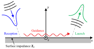
Figure 1: Reception, guidance, and launch of an incident beam by a planar metasurface. The metasurface at $y=0$ is impenetrable and characterized by a position-dependent surface impedance $\mathbf{Z}_{s}$.

Figure 1 illustrates the design problem for an impenetrable metasurface under consideration. In free space, a known beam wave illuminates a planar impenetrable surface in the $xz$-plane. Using a passive, lossless metasurface, it desired that the incident beam is first received and converted into an SW, subsequently guided along the surface, before it is launched back into space from a location that is electrically far separated from the receiving point. The power of the desired output wave is the same as that of the incident beam. Furthermore, a surface with reciprocal parameters is desired.

At the heart of the design lies perfect conversion of a PW into an SW and a subsequent transition into lossless guiding along the surface. Launching is a reciprocal process of receiving and a planar structure with a uniform reactive surface impedance can guide an SW without loss. For such a converter based on the generalized Snell’s law, it was found that an SW, once generated, cannot propagate along the gradient metasurface without suffering secondary scattering by the same metasurface back into space. This lowers the conversion efficiency for electrically long converters Qu et al. (2013), defined for the power accepted by a homogeneous guiding metasurface. The conversion efficiency is significantly improved by introducing a meta-coupler at a height over a homogeneous surface that supports a surface wave Sun et al. (2016). A drawback of this approach is an increased overall thickness. Nevertheless, the conversion efficiency cannot reach 100% because some of the generated SW fields still undergo secondary scattering by the meta-coupler.

Instead of relying on the generalized reflection law, designing the exact SW tailored to the incident wave can lead to a metasurface design that is capable of perfect PW-to-SW conversion. With respect to the chosen guided direction (the $+x$-axis direction in Fig. 1), this custom SW must have a position-dependent amplitude profile such that the amplitude grows over the range of beam illumination due to PW-to-SW conversion, stays constant over the guided range without leakage radiation, then diminishes over the range of beam launch due to SW-to-PW conversion. Over the beam receiving range, the PW is continuously converted into the SW, so there is no abrupt junction between conversion and guiding ranges. The exact profile of the SW is determined such that the PW-to-SW conversion is done in a locally lossless manner, without loss in or power supplied by the metasurface, everywhere on the surface. Once the exact SW is designed, the boundary condition for the impenetrable surface is found for supporting the envisioned total fields as a reactive surface impedance.

In this work, the same polarization is chosen between the input and output beams. For the surface wave, an orthogonal polarization is chosen as in Kwon and Tretyakov (2017); Tcvetkova et al. (2017). An orthogonally polarized SW avoids creating an interference power pattern between the PW and SW on the surface, simplifying the SW synthesis significantly. In the following sections, beam controlling metasurfaces in two-dimensional (2-D) configurations with PWs in the TE polarization (with respect to $y$) and SWs in the TM polarization are presented.

III Impenetrable surface characterization

Let us adopt and suppress an $e^{j\omega t}$ time convention for the following time-harmonic analysis at an angular frequency $\omega$. Referring to Fig. 1, the total fields $\mathbf{E}=\hat{x}E_{x}+\hat{y}E_{y}+\hat{z}E_{z}$, $\mathbf{H}=\hat{x}H_{x}+\hat{y}H_{y}+\hat{z}H_{z}$ in $y\geq 0$ comprise a superposition of those from the incident beam, the SW bound to the metasurface at $y=0$, and the output beam. For an impenetrable surface characterized by a surface impedance $\mathbf{Z}_{s}$, the tangential electric and magnetic fields on the surface, $\mathbf{E}_{t}=\hat{x}E_{tx}+\hat{z}E_{tz}$ and $\mathbf{H}_{t}=\hat{x}H_{tx}+\hat{z}H_{tz}$, are related by

$$\mathbf{E}_{t}=\mathbf{Z}_{s}\mathbf{J}_{s}=\mathbf{Z}_{s}\hat{n}\times\mathbf{H}_{t},$$ (1)

where $\hat{n}=\hat{y}$ is the unit surface normal and $\mathbf{J}_{s}=\hat{n}\times\mathbf{H}_{t}$ is the induced electric surface current density at $y=0$. The rank-2 tensor $\mathbf{Z}_{s}$ may be written as a 2×2 matrix in the $xy$-plane.

Toward arriving at a lossless and reciprocal surface specification, consider $\mathbf{Z}_{s}$ in terms of a reactance tensor $\mathbf{X}_{s}$ written by

$$\mathbf{Z}_{s}=j\mathbf{X}_{s}=j\begin{bmatrix}X_{xx}&X_{xz}\\ X_{zx}&X_{zz}\end{bmatrix},$$ (2)

where the four reactance elements are real. Using (2) in (1), matching both the real and imaginary parts on the two sides uniquely determines the four tensor elements as Kwon and Tretyakov (2017)

$$\mathbf{X}_{s}=\frac{1}{\operatorname{Im}\{H_{tx}H_{tz}^{*}\}}\begin{bmatrix}\operatorname{Re}\{E_{tx}H_{tx}^{*}\}&\operatorname{Re}\{E_{tx}H_{tz}^{*}\}\\ \operatorname{Re}\{E_{tz}H_{tx}^{*}\}&\operatorname{Re}\{E_{tz}H_{tz}^{*}\}\end{bmatrix}.$$ (3)

This reactance tensor represents a lossless, reciprocal surface if the off-diagonal terms are equal to each other. This condition is equivalent to Kwon and Tretyakov (2017)

$$S_{n}=\hat{y}\cdot\frac{1}{2}\operatorname{Re}\{\mathbf{E}_{t}\times\mathbf{H}_{t}^{*}\}=0,$$ (4)

where $S_{n}$ is the normal component of the Poynting vector on the surface. Hence, if there is no net power penetrating the surface at a given point either as absorption by the surface $(S_{n}<0)$ or as power injected into $y>0$ by a source on the surface$(S_{n}>0)$, the surface is locally lossless and reciprocal. If (4) is satisfied everywhere, the metasurface is lossless and reciprocal globally.

The reactance tensor of a lossless surface is in general a Hermitian tensor. Therefore, a real, symmetric tensor in (3) under the condition (4) is not the unique solution for a lossless, reciprocal surface that supports $(\mathbf{E},\mathbf{H})$ because the off-diagonal elements were set to have no imaginary parts by design. Still, a symmetric $\mathbf{X}_{s}$ with real-valued elements is advantageous because its eigenvalues are real and the eigenvectors are orthogonal, allowing realization using an array of rotated resonant meta-atoms.

IV Synthesis of the surface wave

In Fig. 1, consider a 2-D configuration where the input and output PW fields are TE-polarized and the SW field is TM-polarized with all the fields invariant along the $z$-axis. Then, $E_{z}(x,y)$ and $H_{z}(x,y)$ uniquely determine all remaining field components in the $xy$-plane for the TE and TM polarizations, respectively. The electromagnetic uniqueness theorem allows the fields in the half space $y\geq 0$, which is bounded by the metasurface and subject to the radiation condition at infinity, to be uniquely determined from those on the metasurface at $y=0$. Furthermore, the planar metasurface geometry makes analysis and design in the spectral domain efficient via Fourier transform. Derivations for field components and the normal component of the Poynting vector are available in Appendices A and B for TE- and TM-mode fields, respectively.

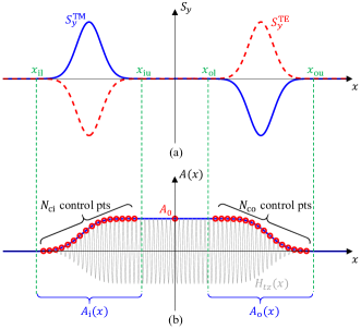
Figure 2: Illustration of power and envelope profiles for SW synthesis. (a) The normal component of the Poynting vector for the TE- and TM-polarized fields. (b) The envelope design for the TM-polarized SW component, $H_{tz}(x)$.

The metasurface design starts from a complete knowledge of the incident beam and the desired output beam. For a given input beam, we assume that the output PW fields are known from a separate overall function design of the metasurface. In particular, the total output power should be equal to the input power in order to make the overall system lossless. In terms of $E_{tz}(x)$ and its Fourier transform $\tilde{E}_{tz}(k_{x})=\mathscr{F}\{E_{tz}(x)\}$, the expression for the normal component of the time-average Poynting vector is given in (26), which can be written compactly as

$$S^{\text{TE}}_{y}(x)=\frac{1}{2k\eta}\operatorname{Re}\left\{E_{tz}^{*}(x)\mathscr{F}^{-1}\left[k_{y}\tilde{E}_{tz}(k_{x})\right]\right\}.$$ (5)

Typically, closed-form field expressions are approximate and available only in the paraxial region near the beam axis, even for commonly studied beams such as Gaussian or Bessel beams. Hence, the primary quantities for analysis and design are $z$-directed field components on the metasurface in this study.

For the TE-polarized input and output fields in a typical beam control application described in Fig. 1, the normal power density profile is illustrated in Fig. 2(a) as a red dashed curve. For a beam wave having a finite support, we can define the lower and upper $x$-limits for the input wave, $x_{\text{il}}$ and $x_{\text{iu}}$, such that non-negligible fields and power are observed in $x\in[x_{\text{il}},x_{\text{iu}}]$. Similarly, two $x$-coordinates are set to define the range where the output beam leaves the surface to be $x\in[x_{\text{ol}},x_{\text{ou}}]$. Over the illuminated range, $S^{\text{TE}}_{y}(x)<0$. Over the beam launch range, $S^{\text{TE}}_{y}(x)>0$.

The objective of the SW synthesis is to design a custom SW, specified by $H_{tz}(x)$ in $-\infty<x<\infty$, such that (4) is satisfied for all $x$. Choosing an orthogonal TM polarization for the SW makes the normal Poynting vector component of the total fields equal to an algebraic sum of the TE and TM polarization components, i.e.,

$$S_{n}(x)=S^{\text{TE}}_{y}(x)+S^{\text{TM}}_{y}(x).$$ (6)

The expression for the TM-mode Poynting vector component, shown in (30), can be written concisely as

$$S^{\text{TM}}_{y}(x)=\frac{\eta}{2k}\operatorname{Re}\left\{H_{tz}^{*}(x)\mathscr{F}^{-1}\left[k_{y}\tilde{H}_{tz}(k_{x})\right]\right\}.$$ (7)

In Fig. 2(a), the target power profile for the TM-polarized SW is shown as a solid blue curve. For $H_{tz}(x)$, we choose propagating function in the $+x$ direction with a custom $x$-dependent envelope. This envelope function is a real function, taking non-negative values. It is denoted by $A(x)$ and shown as a blue curve in Fig. 2(b). Spatially, no SW is present to the left of the illumination range in $x<x_{\text{il}}$ and past the launch range of the output PW in $x>x_{\text{ou}}$. Between complete reception of the incident beam and initiation of the output beam launch, in $x\in(x_{\text{iu}},x_{\text{ol}})$, the SW propagates in the $+x$-direction, carrying the received power without attenuation or growth. During reception in $x\in[x_{\text{il}},x_{\text{iu}}]$, the envelope monotonically increases as power is gradually accumulated for the SW as the input PW is converted into the SW. The reverse process occurs in the launch range $x\in[x_{\text{ol}},x_{\text{ou}}]$. Hence, we express the envelope function as

$$A(x)=\begin{cases}0,&x<x_{\text{il}}\ \ \text{or}\ \ x>x_{\text{ou}}\\ A_{\text{i}}(x),&x_{\text{il}}\leq x\leq x_{\text{iu}}\\ A_{0},&x_{\text{iu}}<x<x_{\text{ol}}\\ A_{\text{o}}(x),&x_{\text{ol}}\leq x\leq x_{\text{ou}}\end{cases},$$ (8)

where $A_{\text{i}}(x)$ is an increasing function associated with the reception, $A_{\text{o}}(x)$ is a decreasing function associated with the launch, and $A_{0}$ is a constant. Once $A(x)$ is specified, the tangential magnetic field component on the surface is defined as

$$H_{tz}(x)=A(x)e^{-jk_{\text{c}}x},$$ (9)

where $k_{\text{c}}$ is the center (or “carrier”) wavenumber of the SW chosen in the invisible range $(k_{\text{c}}>k)$ so that the synthesized TM wave propagates while bound to the metasurface. A snapshot of $H_{tz}(x)$ (the real part) is visualized as a thin gray curve in Fig. 2(b). It is stressed that $H_{tz}(x)$ in (9) is defined on the surface $(y=0)$ only. In order to obtain the associated fields that are valid (i.e., Maxwellian) in the entire volume of existence $(y\geq 0)$, we express $H_{tz}(x)$ as a superposition of homogeneous and inhomogeneous plane wave components evaluated at $y=0$, using Fourier expansions.

At this point, it is instructive to assess the qualitative behavior of the synthesized SW in $y\geq 0$. The definition of $H_{tz}(x)$ with respect to the envelope $A(x)$ in (9) relates their Fourier transforms as

$$\tilde{H}_{tz}(k_{x})=\tilde{A}(k_{x}-k_{c}).$$ (10)

Since $A(x)$ is a real, non-negative function of $x$, $\tilde{A}(k_{x})$ has the maximum at $k_{x}=0$. While a finite spatial support of $A(x)$ makes $\tilde{A}(k_{x})$ not completely vanish at large $|k_{x}|$, the effective spectral width of $\tilde{A}(k_{x})$ is inversely proportional to the range of non-zero $A(x)$. From (27), the resulting H-field component of the SW in $y\geq 0$ is expressed as

$$H_{z}(x,y)=\frac{1}{2\pi}\int\limits_{-\infty}^{\infty}\tilde{A}(k_{x}-k_{c})e^{-j(k_{x}x+k_{y}y)}dk_{x}.$$ (11)

It can be seen that the dominant contribution to $H_{z}(x,y)$ comes from its spectrum at and around $k_{x}=k_{c}$. At $k_{x}=k_{c}$, the integrand in (11) represents a surface wave bound to the $y=0$ surface with a positive propagation constant of $k_{x}=k_{c}$ in the $x$-direction and an attenuation constant of $|k_{y}|=\sqrt{k_{c}^{2}-k^{2}}$ in the $y$-direction. Over the beam reception and launch ranges, the amplitude of the SW grows and diminishes gradually with respect to $x$, respectively. In both ranges, the SW propagates in the $+x$-direction and attenuates exponentially in the $+y$-direction. Finally, contributions from all other spectral ranges make the SW exist over the intended, finite range of $x$.

Requiring $A(x)$ to be a continuous function, it remains to determine the functions, $A_{\text{i}}(x)$ and $A_{\text{o}}(x)$, and the constant $A_{0}$. For $A_{\text{i}}(x)$, we choose a closely spaced set of $N_{\text{ci}}$ control points of values $A_{n}$ at locations $x=x_{\text{c}n}$ $(n=-N_{\text{ci}},-N_{\text{ci}}+1,\ldots,-1)$. Similarly, $N_{\text{co}}$ number of control points of values $A_{n}$ at $x=x_{\text{c}n}$ $(n=1,2,\ldots,N_{\text{co}})$ are defined for $A_{\text{o}}(x)$. The constant level at $A_{0}$ should make smooth connections to the transition ranges on both sides. A continuous envelope function is then defined using these control points (locations and values) via interpolation. No control points are assigned at the boundary locations of the input and output beam ranges. In Fig. 2(b), control points are indicated by red circles. The number and $x$-locations of the control points are set appropriately by the designer depending on the allowed complexity of the synthesized SW.

Efficient numerical optimizations can determine the values of $A_{n}$ $(n=-N_{\text{ci}},\ldots,N_{\text{co}})$. In this work, a square error function defined by

$$\text{error}=\int\limits_{-\infty}^{\infty}|S^{\text{TE}}_{y}(x)+S^{\text{TM}}_{y}(x)|^{2}dx$$ (12)

is minimized with respect to the $N_{\text{ci}}+N_{\text{co}}+1$ number of control point values. Specifically, a gradient-free optimization method available through the fminsearch function in Matlab has been used for all designs presented in Sec. V. After some adjustments to the number and locations of control points, all optimizations converged within a convergence tolerance of $10^{-6}$ relative to the error associated with a null initial guess.

Once the optimized envelope function $A(x)$ is determined, using $H_{tz}(x)$ from (9) in (28) at $y=0$ finds $E_{tx}(x)$. Together with $E_{tz}(x)$ and $H_{tx}(x)$ given by the TE-mode fields, they determine the surface reactance tensor that achieves the designed beam control via (3).

Since a spatially varying envelope function is used, the synthesized SW has a continuum of spectrum concentrated around $k_{x}=k_{\text{c}}$ rather than a discrete spectrum. As a result, some of the spectrum will spill into the visible region $(|k_{x}|<k)$. This means that satisfaction of (4) for all $x$, or equivalently the resulting passive, lossless metasurface, necessarily entails excitation of extra PW components in order to to perform the required beam manipulation. The amount of TM-polarized PW components can be assessed by evaluating the total TM-mode power per unit length in the $z$-axis direction that escapes the metasurface. This power, denoted $P^{\text{TM}}_{y}$, is found to have a spectral integral representation given by

$$P^{\text{TM}}_{y}=\int\limits_{-\infty}^{\infty}S^{\text{TM}}_{y}(x)dx=\int\limits_{-\infty}^{\infty}\operatorname{Re}\left\{\frac{\eta k_{y}}{4\pi k}|\tilde{H}_{tz}(k_{x})|^{2}\right\}dk_{x}.$$ (13)

It can be seen that non-zero TM-mode spectrum in the visible region leads to some TM-mode power that is not bound to the metasurface. In principle, this amount of TM-polarized PW components can be reduced to approach zero by increasing $k_{\text{c}}$ deep into the invisible range. However, this results in faster spatial variations for the surface impedance tensor elements, making an accurate realization more challenging.

V Design examples

In the following examples, a metasurface design is characterized as a tensor surface impedance $\mathbf{Z}_{s}(x)$, given in terms of the reactance tensor elements in (2). In numerical validations using COMSOL Multiphysics, the impedance boundary condition (1) is enforced at $y=0$.

V.1 Gaussian beam translator-reflector

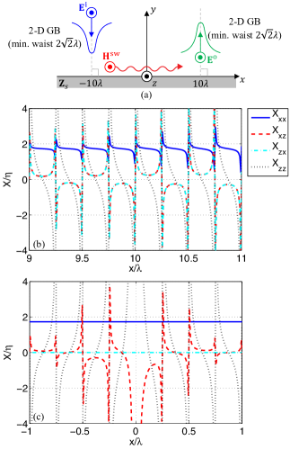
Figure 3: A GB translator-reflector design. (a) The design requirement. A normally incident GB is routed by the metasurface before it is launched normally. Beam axes are indicated by gray dashed lines. The designed $\mathbf{X}_{s}$ elements (b) over an SW-to-PW conversion range and (c) over a guided SW propagation range.

As a first design example, a translator-reflector for receiving and launching a Gaussian beam (GB) propagating normal to the metasurface is presented. The specific design function is illustrated in Fig. 3(a). A 2-D GB propagating in the $-y$-axis direction illuminates the metasurface with the beam axis aimed at $x=-10\lambda$, where $\lambda$ is the free-space wavelength. The output beam is a GB of the same beam specification that is launched normally into free space from $x=10\lambda$, after being translated in the $+x$-axis direction. The tangent vector of the input electric field on the surface is specified by

$$\mathbf{E}^{\text{i}}_{t}(x)=\mathbf{E}^{\text{i}}_{0}e^{-(x+10\lambda)^{2}/2\sigma^{2}};\ \ \mathbf{E}^{\text{i}}_{0}=\hat{z}~{}\text{V/m},\ \sigma=2\lambda.$$ (14)

Equation (14) completely specifies the incident fields in $y\geq 0$. The minimum waist of the input beam is equal to $\sqrt{2}\sigma=2\sqrt{2}\lambda$ and it is located in the $xz$-plane. The tangential vector of the output beam is specified to be

$$\mathbf{E}^{\text{o}}_{t}(x)=\mathbf{E}^{\text{o}}_{0}e^{-(x-10\lambda)^{2}/2\sigma^{2}},\ \ \mathbf{E}^{\text{o}}_{0}=\hat{z}~{}\text{V/m}.$$ (15)

The same amplitude vector and beam waist guarantee that the output power per unit length in $z$ is equal to that of the input beam.

For each beam, we treat the decayed fields at positions away from the beam axis by more than $3\sigma$, where the field amplitude reduces to 1.1% of the peak value, as zero and thus choose $x_{\text{il}}=-16\lambda$, $x_{\text{iu}}=-4\lambda$, $x_{\text{ol}}=4\lambda$, and $x_{\text{ou}}=16\lambda$. Next, the center wavenumber is chosen to be $k_{\text{c}}=2k$. Due to the symmetry of the problem, an even symmetry for $A(x)$ is enforced with respect to $x$. A total of 17 independent control points, $A_{n}$ $(n=-16,-15,\ldots,-1)$ in $x\in[x_{\text{il}},x_{\text{iu}}]$ and $A_{0}$ at $x=0$, are assigned. An equal spacing was chosen between the 16 points, $x_{n}$ $(n=-16,-15,\ldots,-1)$. Numerical optimization was performed for the 17 control point values. In fact, the power profiles and envelope function shown in Fig. 2 display the optimization results of this design drawn to scale. As can be observed in Fig. 2(a), $S^{\text{TE}}_{y}$ and $S^{\text{TM}}_{y}$ effectively cancel each other. For the optimized envelope, it was found that $A_{0}=16.5~{}\text{mA/m}$ and other values scale according to Fig. 2(b).

The elements of $\mathbf{X}_{s}$ of the optimized design were computed over $-20\lambda<x<20\lambda$. Figure 3(b) shows its four elements in $9\lambda<x<11\lambda$, where SW-to-PW conversion occurs. They are highly spatially dispersive functions. The values diverge four times over one wavelength, where the denominator in (3) becomes zero. The spatial frequency of diverging reactance elements is a result of the choice $k_{\text{c}}$ combined with the uniform phase of $H_{tx}$ associated with broadside launching. As expected for a lossless design, it is observed that $X_{xz}=X_{zx}$. In comparison, the $x$-range near the origin corresponds to guidance of a TM wave in the absence of any TE components. The reactance elements over $-\lambda<x<\lambda$ are plotted in Fig. 3(c). Here, with only a TM-mode SW present, it is noted that $H_{tx}=0$, $E_{tz}=0$, and $\operatorname{Re}\{E_{tx}H_{tz}^{*}\}=0$ in (3). A tensor impedance representation is not appropriate in such a case. In numerical evaluation, (3) may be understood as a limiting case where TE-polarized components approach zero. Still, some numerical artifact is observed in that $X_{xz}\neq X_{zx}$ in Fig. 3(c). Since there are no TE-polarized components in this range, only the terms $X_{xx}$ and $X_{zx}$ are significant. Since $X_{zx}=0$, no $z$-directed (TE-polarized) electric field will be generated from an $x$-directed electric current. A constant inductive self-reactance at $X_{xx}=1.73\eta$ is consistent with a TM-mode surface wave having a propagation constant of $k_{\text{c}}=2k$. In the guided TM-polarized SW range, the tensor surface impedance may well be replaced by an isotropic reactive impedance $\mathbf{Z}_{s}=\mathbf{I}_{t}jX_{xx}$ $(\mathbf{I}_{t}=\text{an identity tensor in the $xy$-plane})$. This isotropic choice of $\mathbf{Z}_{s}$ over the constant-amplitude SW range, $x_{\text{iu}}<x<x_{\text{ol}}$, was also tested in numerical analysis. The resulting field distributions (not shown) are found to be the same as the case where the fully-anisotropic impedance was used.

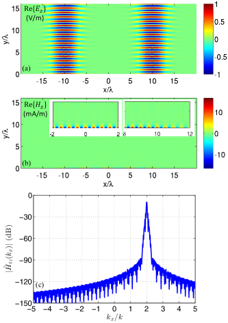
Figure 4: Simulated performance of the GB translator-reflector metasurface. (a) A snapshot of $E_{z}(x,y)$. (b) A snapshot of $H_{z}(x,y)$. (c) $|\tilde{H}_{tz}(k_{x})|$.

The scattering characteristics of the metasurface is simulated using COMSOL Multiphysics. Illuminated by the GB the metasurface was designed for, Fig. 4(a) plots a snapshot of $E_{z}$ over an area of $|x|<20\lambda$, $0<y<16\lambda$. Over the illuminated range by the input GB, no reflection is seen with only the incident beam field being observed. In the output GB launch range, the desired GB with the same strength and beam waist is radiated. A snapshot of $H_{z}$ is shown in Fig. 4(b). Non-zero fields are observed tightly bound to the $y=0$ surface. In the inset on the right, a magnified view of the $H_{z}$ snapshot is shown over $8\lambda<x<12\lambda$ in the SW-to-PW conversion range. A surface wave with a diminishing amplitude is induced as designed. Over the guided SW range shown in the inset on the left, a TM-polarized SW of a constant amplitude is clearly visible. Over the input beam reception range (a magnified view not shown), the amplitude of the SW gradually grows. In Fig. 4(c), the magnitude of the SW field spectrum is plotted with respect to $k_{x}$ in both the visible $(|k_{x}|\leq k)$ and invisible $(|k_{x}|>k)$ ranges. The spectrum is strongly concentrated around the maximum at $k_{x}=k_{\text{c}}=2k$. The shape of the SW spectrum is completely determined by the envelope function because $\tilde{H}_{tz}(k_{x})=\mathscr{F}\{A(x)e^{-jk_{\text{c}}x}\}=\tilde{A}(k_{x}-k_{\text{c}})$. Computed using (13), the power associated with the TM-polarized PW component from the visible range is six orders of magnitude below that of the input GB power. Hence, the synthesized TM-polarized SW can be considered completely bound to the reflecting surface.

V.2 Probe current-fed Gaussian beam launcher

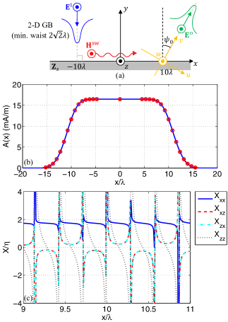
Figure 5: Design of an oblique GB launcher. (a) An underlying configuration of a beam launcher fed by an input beam. (b) The envelop function $A(x)$ and the control points for $\psi_{0}=30\degree$. (c) The reactance tensor elements in the launch range.

A uniform-amplitude SW can be generated by a localized source. Via reciprocity, an SW can be absorbed by a localized lossy material or load impedance. When combined with the PW-to-SW conversion, such a device represents a leaky-wave antenna that transmits or receives a beam wave.

Here, a GB launcher in an oblique angle is designed. For this purpose, the GB translator-reflector of Sec. V.1 can be adapted to design an oblique GB launcher excited by an input beam, before the SW feeding mechanism is replaced with a localized current probe. The underlying GB launcher configuration is illustrated in Fig. 5(a). The input beam remains unchanged from the translator-reflector design in Sec. V.1. The output beam shape remains the same, but it is launched at an angle of $\psi_{0}$ from the surface normal from $x=10\lambda$. The output beam can be first characterized in a rotated $(u,v,w)$ coordinate system with respect to $z=w$ such that the $v$-axis is aligned with the output beam axis. Along the $u$-axis, the output GB is completely characterized by the $w$-component of the electric field

$$\mathbf{E}^{\text{o}}_{t}(u)=\mathbf{E}^{\text{o}}_{0}e^{-u^{2}/2\sigma^{2}},\ \ \mathbf{E}^{\text{o}}_{0}=\hat{w}~{}\text{V/m}.$$ (16)

Then, the output beam fields in the entire $uv$-plane can be obtained by applying the relations in Appendix A in the $uv$-plane. A special care should be exercised so that the fields in the range $v<0$ represent a propagating wave with $k_{v}>0$. This can be done by taking a complex conjugate of the fields from Appendix A, corresponding to a time-reversal transformation. Fields evaluated along the $x$-axis in the $uv$-plane can be transformed to the $xyz$ system by a proper coordinate rotation, before they can be used for the device design in the $xy$-plane.

For a 30° GB launcher $(\psi_{0}=30\degree)$, the $x$-range of numerical synthesis of the envelope function was set with $x_{\text{il}}=-16\lambda$, $x_{\text{iu}}=-4\lambda$, $x_{\text{ol}}=3.75\lambda$, and $x_{\text{ou}}=16.25\lambda$. For the output beam, the range was slightly extended to account for the oblique launch angle. In each of $x\in[x_{\text{il}},x_{\text{iu}}]$ and $x\in[x_{\text{ol}},x_{\text{ou}}]$, 15 equally-spaced control points were assigned. Hence, together with $A_{0}$ assigned to $x=0$, a total of 31 control points were defined for $A(x)$ and they were optimized for the minimum square error (12). The center wavenumber was chosen to be $k_{\text{c}}=2k$. The optimized envelope function together with the control points are plotted in Fig. 5(b). The amplitude of the guided SW was found to be $A_{0}=16.5~{}\text{mA/m}$, which remains unchanged from the translator-reflector design in Sec. V.1 as can be expected. In Fig. 5(c), the reactance tensor elements over $9\lambda<x<11\lambda$ in the oblique GB launch range are plotted. They are different from Fig. 3(b) and they diverge less frequently with respect to $x$. This is due to different phase gradients present in $H_{tx}$ in (3) for the same SW expected in the two designs. Indicative of a lossless property, $X_{xz}=X_{zx}$ is observed.

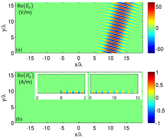
Figure 6: Simulation results for the oblique GB launcher. (a) A snapshot of $E_{z}(x,y)$. (b) A snapshot of $H_{z}(x,y)$.

Since launching the output GB using a localized source is of interest, we adopt a localized source in the form of a two-element array around $x=0$. In other words, the $+x$-propagating constant-amplitude SW near $x=0$ is provided by a current probe instead of an input GB. Two elementary radiators separated by a quarter wavelength with a 90° phase difference can create a unidirectional radiation pattern Balanis (2005). Hence, denoting the attenuation constant of the SW around $x=0$ by $\alpha_{\text{c}}$, we use an impressed electric current source given by

$$\mathbf{J}_{\text{imp}}=\hat{y}J_{0}e^{-\alpha_{\text{c}}y}\left[\delta\left(x+\frac{\lambda_{\text{c}}}{8}\right)e^{j\frac{\pi}{4}}+\delta\left(x-\frac{\lambda_{\text{c}}}{8}\right)e^{-j\frac{\pi}{4}}\right]$$ (17)

in $0\leq y\leq\lambda_{\text{c}}/4$ and zero in $y>\lambda_{\text{c}}/4$, where $\lambda_{\text{c}}=2\pi/k_{\text{c}}$ is the guided wavelength of the SW. This model represents two strips of vertical electric current of a $\lambda_{\text{c}}/4$ height. Their $y$-dependence is matched to that of the TM SW for maximum coupling. In simulation results that follow, $J_{0}=1~{}\text{A/m}$ has been used.

Snapshots of the $z$-component of the total electric and magnetic fields are plotted in Fig. 6. In Fig. 6(a), a GB is launched from $x=10\lambda$ at an angle of 30° as desired. In the snapshot of $H_{z}$ in Fig. 6(b), the TM-mode wave is visible only as an evanescent wave bound to the surface. The left inset shows a magnified view near the two-element current source at $x=0$. The two short line segments in black indicate the source positions and their height. A constructive interference between the fields generated by the two strip currents produces a $+x$-propagating SW with a maximum amplitude of 1 A/m (realized on the surface) as designed. A destructive interference results in negligible excitation of an SW toward the $-x$-axis direction. The inset on the right shows a portion of the SW-to-PW conversion range. The SW amplitude is gradually reduced with increasing $x$ due to continuous leakage into space.

V.3 Gaussian beam-excited focusing lens

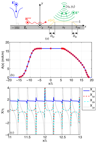
Figure 7: A flat lens excited by an input GB. (a) The GB-to-SW-to-converging wave transformation configuration. (b) The envelope function $A(x)$ and the 38 control points of the optimized design. (c) The reactance tensor elements in the cylindrical wave launch range.

In order to demonstrate the versatility of the design technique, a focusing lens excited by the same normally incident GB considered in Sec. V.1 is designed. The desired wave transformation is illustrated in Fig. 7(a). A normally incident GB is converted into a TM-polarized SW in $x<0$. The converted SW is transformed into a converging cylindrical wave in the range $x_{\text{ol}}<x<x_{\text{ou}}$, where an envelop function $e(x)$ for $|E_{tz}(x)|$ is introduced. On both ends within the range, a transition period of a length $D_{\text{tr}}$ in a raised cosine profile is defined for a smooth transition between unity and zero, as illustrated in Fig. 7(a). Specifically,

$$e(x)=\begin{cases}0,&x<x_{\text{ol}}\ \ \text{or}\ \ x\geq x_{\text{ou}}\\ [1-\cos(\frac{x-x_{\text{ol}}}{D_{\text{tr}}/\pi})]/2,&x_{\text{ol}}\leq x<x_{\text{ol}}+D_{\text{tr}}\\ 1,&x_{\text{ol}}+D_{\text{tr}}\leq x<x_{\text{ou}}-D_{\text{tr}}\\ [1-\cos(\frac{x-x_{\text{ou}}}{D_{\text{tr}}/\pi})]/2,&x_{\text{ou}}-D_{\text{tr}}\leq x<x_{\text{ou}}\end{cases}.$$ (18)

In order for the launched cylindrical wave to converge at a focal point $(x_{\text{f}},y_{\text{f}})$, a phase distribution for $E_{tz}$ is introduced as

$$\phi(x)=k\sqrt{(x-x_{\text{f}})^{2}+y_{\text{f}}^{2}}+\phi_{0},$$ (19)

where $\phi_{0}$ is an arbitrary phase constant. Then, the tangential electric field for the output wave is defined to be

$$\mathbf{E}^{\text{o}}_{t}(x)=\mathbf{E}^{\text{o}}_{0}e(x)e^{j\phi(x)},\ \ \mathbf{E}^{\text{o}}_{0}=\hat{z}E^{\text{o}}_{0}.$$ (20)

The amplitude $E^{\text{o}}_{0}$ is determined to make the overall conversion from the input GB to the output focusing wave lossless.

For the TE-polarized GB input wave considered in Sec. V.1, a focusing lens with a focal point at $(x_{\text{f}},y_{\text{f}})=(12\lambda,10\lambda)$ is designed using an SW-to-PW conversion range with $x_{\text{ol}}=5\lambda$, $x_{\text{ou}}=19\lambda$. With a choice of $D_{\text{tr}}=2\lambda$, the $x$-range of a constant-amplitude electric field for the output wave is $7\lambda<x<17\lambda$. The phase constant $\phi_{0}$ is set to zero. For this chosen profile of $\mathbf{E}^{\text{o}}_{t}(x)$, by setting the output PW power equal to the input GB power, the amplitude is found to be $E^{\text{o}}_{0}=0.569~{}\text{V/m}$. Next, $N_{\text{ci}}=15$ control points are defined for the input range $-16\lambda<x<-4\lambda$, four control points are assigned to both transition ranges in the output range. To the constant-amplitude range of $10\lambda$ length, 14 control points are assigned. The total number of control points is 38 for this lens design. The envelop function $A(x)$ of the optimized design is shown in Fig. 7(b) together with the control points indicated by red circles. In $7\lambda<x<17\lambda$, where a TE-polarized aperture electric field of a uniform magnitude is synthesized, it is observed that $A(x)$ diminishes with an increasingly negative slope with respect to $x$ as the SW power is continuously lost to the output PW. The four reactance element values of the optimized design over $11\lambda<x<13\lambda$ in the SW-to-PW conversion range are shown in Fig. 7(c) as highly spatially dispersive functions. The lossless nature of the metasurface lens is indicated by the fact $X_{xz}=X_{zx}$.

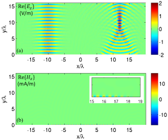
Figure 8: Simulation results for the flat focusing lens excited by GB illumination. (a) A snapshot of $E_{z}(x,y)$. (b) A snapshot of $H_{z}(x,y)$.

Figure 8 shows the simulated results for the lens obtained using COMSOL Multiphysics. A snapshot of the TE-component of the electric field is plotted in Fig. 8(a). Converging cylindrical waves form a focal point at $(x,y)=(x_{\text{f}},y_{\text{f}})=(12\lambda,10\lambda)$ as designed. A snapshot of $H_{z}(x,y)$ in Fig. 8(b) shows the TM-polarized field, which is tightly bound to the metasurface. In a magnified view in the range $15\lambda<x<19\lambda$, the SW wave is seen to be diminishing and disappearing as all of its guided power along the $+x$-direction is leaked into the PW spectrum.

VI Conclusion

Arbitrary polarization-preserving beam control using passive, lossless impenetrable metasurfaces has been presented. It is based on a custom SW in an orthogonal polarization designed to propagate along the surface. By finding an optimal spatial envelope for the SW such that there is zero normal component for the Poynting vector everywhere on the surface, a lossless metasurface can convert a PW into an SW, guide the SW unattenuated along the surface, and launch a PW via an SW-to-PW transformation. As specific design examples, a GB translator-reflector, a GB launcher excited by a localized source, and a GB-fed flat focusing lens have been presented. Lossless metasurfaces characterized by a reactance tensor in a plane may be realized using an array of rotated subwavelength resonators printed on a grounded dielectric substrate.

Availability of an orthogonal polarization for SW synthesis simplifies the design process owing to the orthogonality of power flow in the surface normal direction between the PW and SW on the metasurface. The same design approach can be envisioned for polarization-converting transformations between the input and output beams or for using an SW that is co-polarized with the input and output beams. SW synthesis in such a scenario is expected to be challenging due to the complex interference power pattern created by the co-polarized PW and SW components in the system.

At microwave frequencies, a planar array of rotated anisotropic printed conductor patch resonators on a grounded dielectric substrate is a promising configuration Fong et al. (2010); Minatti et al. (2012); Patel and Grbic (2013); Lee and Sievenpiper (2016) that allows accurate, low-cost fabrication for realizing the inhomogeneous, tensor surface impedances in this study.

Appendix A Spectral representations of fields and power density in TE polarization

For TE-polarized fields, the tangential electric field on the surface, $E_{tz}(x)=E_{z}(x,y=0)$, is expressed as an inverse Fourier transform of its spectrum $\tilde{E}_{tz}(k_{x})$ as

$$E_{tz}(x)=\mathscr{F}^{-1}[\tilde{E}_{tz}(k_{x})]=\frac{1}{2\pi}\int\limits_{-\infty}^{\infty}\tilde{E}_{tz}(k_{x})e^{-jk_{x}x}dk_{x},$$ (21)

where $k_{x}$ is the wavenumber in the $x$-direction. Here, we add a tilde to a spatial function to indicate its Fourier transform in $x$. Equation (21) represents a superposition of plane waves propagating in the $xy$-plane over the $x$-wavenumber $k_{x}$, evaluated at $y=0$. Hence, at any point $(x,y)$ in $y\geq 0$, the field $E_{z}(x,y)$ is the same superposition of plane waves evaluated at $(x,y)$ after a proper phase delay in the $y$ direction is incorporated to each plane wave component in the integrand of (21). In other words,

$$E_{z}(x,y)=\frac{1}{2\pi}\int\limits_{-\infty}^{\infty}\tilde{E}_{tz}(k_{x})e^{-j(k_{x}x+k_{y}y)}dk_{x},$$ (22)

where

$$k_{y}=\begin{cases}\sqrt{k^{2}-k_{x}^{2}},&|k_{x}|\leq k\\ -j\sqrt{k_{x}^{2}-k^{2}},&|k_{x}|>k\end{cases}$$ (23)

and $k$ is the free-space wavenumber. At an observation point $(x,y)$, (22) represents a superposition of propagating and evanescent plane waves. In (23), a choice of the negative branch for the square root for $|k_{x}|>k$ guarantees an exponential decay toward $y\to\infty$ for each inhomogeneous plane wave component. The associated magnetic field components in $y\geq 0$ are obtained from Maxwell’s curl equations as

$$H_{x}(x,y) = \frac{1}{2\pi}\int\limits_{-\infty}^{\infty}\frac{k_{y}}{k\eta}\tilde{E}_{tz}(k_{x})e^{-j(k_{x}x+k_{y}y)}dk_{x},$$ (24)

$$H_{y}(x,y) = -\frac{1}{2\pi}\int\limits_{-\infty}^{\infty}\frac{k_{x}}{k\eta}\tilde{E}_{tz}(k_{x})e^{-j(k_{x}x+k_{y}y)}dk_{x},$$ (25)

where $\eta$ is the free-space intrinsic impedance.

The normal component of the time-average Poynting vector is the key quantity in the design process. Using $H_{tx}(x)=H_{x}(x,y=0)$ from (24), the $y$-component of the TE-mode Poynting vector is expressed as

$$\begin{split}S^{\text{TE}}_{y}(x)&=\frac{1}{2}\operatorname{Re}\{E_{tz}H_{tx}^{*}\}=\frac{1}{2}\operatorname{Re}\{E_{tz}^{*}H_{tx}\}\\ &=\frac{1}{2}\operatorname{Re}\left\{E_{tz}^{*}(x)\frac{1}{2\pi}\int\limits_{-\infty}^{\infty}\frac{k_{y}}{k\eta}\tilde{E}_{tz}(k_{x})e^{-jk_{x}x}dk_{x}\right\}.\end{split}$$ (26)

For a given profile $E_{tz}(x)$, evaluation of (26) involves two one-dimensional integrals, of which numerical evaluation can be performed efficiently.

Appendix B Spectral representations of fields and power density in TM polarization

Expressions of field components and the normal Poynting vector component in the spectral domain in terms of $H_{tz}(x)=H_{z}(x,y=0)$ are derived following the same procedure as in Appendix A. Here, only the final results are summarized.

In $y\geq 0$, the three TM-mode field components, $H_{z}$, $E_{x}$, and $E_{y}$, are expressed as a superposition of plane waves as

$$H_{z}(x,y) = \frac{1}{2\pi}\int\limits_{-\infty}^{\infty}\tilde{H}_{tz}(k_{x})e^{-j(k_{x}x+k_{y}y)}dk_{x},$$ (27)

$$E_{x}(x,y) = -\frac{1}{2\pi}\int\limits_{-\infty}^{\infty}\frac{\eta k_{y}}{k}\tilde{H}_{tz}(k_{x})e^{-j(k_{x}x+k_{y}y)}dk_{x},$$ (28)

$$E_{y}(x,y) = \frac{1}{2\pi}\int\limits_{-\infty}^{\infty}\frac{\eta k_{x}}{k}\tilde{H}_{tz}(k_{x})e^{-j(k_{x}x+k_{y}y)}dk_{x},$$ (29)

where a tilde notation has been used to indicate the Fourier transform of $H_{tz}(x)$. The expression for the $y$-component of the TM-mode Poynting vector is found to be

$$S^{\text{TM}}_{y}(x)=\frac{1}{2}\operatorname{Re}\left\{H_{tz}^{*}(x)\frac{1}{2\pi}\int\limits_{-\infty}^{\infty}\frac{\eta k_{y}}{k}\tilde{H}_{tz}(k_{x})e^{-jk_{x}x}dk_{x}\right\}.$$ (30)

References

- Holloway et al. (2012) C. L. Holloway, E. F. Kuester, J. A. Gordon, J. O’Hara, J. Booth, and D. R. Smith, “An overview of the theory and applications of metasurfaces: the two-dimensional equivalents of metamaterials,” IEEE Antennas Propag. Mag. 54, 10 (2012).
- Yu et al. (2011) N. Yu, P. Genevet, M. A. Kats, F. Aieta, J.-P. Tetienne, F. Capasso, and Z. Gaburro, “Light propagation with phase discontinuities: generalized laws of reflection and refraction,” Science 334, 333 (2011).
- Aieta et al. (2012) F. Aieta, P. Genevet, N. Yu, M. A. Kats, Z. Gaburro, and F. Capasso, “Out-of-plane reflection and refraction of light by anisotropic optical antenna metasurfaces with phase discontinuities,” Nano Lett. 12, 1702 (2012).
- Pfeiffer and Grbic (2013) C. Pfeiffer and A. Grbic, “Metamaterial Huygens’ surfaces: tailoring wave fronts with reflectionless sheets,” Phys. Rev. Lett. 110, 197401 (2013).
- Wong et al. (2015) J. P. S. Wong, M. Selvanayagam, and G. V. Eleftheriades, “Polarization considerations for scalar Huygens metasurfaces and characterization for 2-D refraction,” IEEE Trans. Microw. Theory Techn. 63, 913 (2015).
- Asadchy et al. (2015) V. S. Asadchy, Y. Ra’di, J. Vehmas, and S. A. Tretyakov, “Functional metamirrors using bianisotropic elements,” Phys. Rev. Lett. 114, 095503 (2015).
- Monticone et al. (2013) F. Monticone, N. Mohammadi Estakhri, and A. Alù, “Full control of nanoscale optical transmission with a composite metascreen,” Phys. Rev. Lett. 110, 203903 (2013).
- Lin et al. (2014) D. Lin, P. Fan, E. Hasman, and M. L. Brongersma, “Dielectric gradient metasurface optical elements,” Science 345, 298 (2014).
- Wang et al. (2015) Q. Wang, X. Zhang, Y. Xu, Z. Tian, J. Gu, W. Yue, S. Zhang, J. Han, and W. Zhang, “A broadband metasurface-based terahertz flat-lens array,” Adv. Opt. Mater. 3, 779 (2015).
- Khorasaninejad et al. (2016) M. Khorasaninejad, W. T. Chen, R. C. Devlin, J. Oh, A. Y. Zhu, and F. Capasso, “Metalenses at visible wavelengths: Diffraction-limited focusing and subwavelength resolution imaging,” Science 362, 1190 (2016).
- Ni et al. (2013) X. Ni, A. V. Kildishev, and V. M. Shalaev, “Metasurface holograms for visible light,” Nat. Commun. 4, 2087 (2013).
- Huang et al. (2013) L. Huang, X. Chen, H. Mühlenbernd, H. Zhang, S. Chen, B. Bai, Q. Tan, G. Jin, K.-W. Cheah, C.-W. Qiu, J. Li, T. Zentgraf, and S. Zhang, “Three-dimensional optical holography using a plasmonic metasurface,” Nat. Commun. 4, 2808 (2013).
- Genevet et al. (2012) P. Genevet, N. Yu, F. Aieta, J. Lin, M. A. Kats, R. Blanchard, M. O. Scully, Z. Gaburro, and F. Capasso, “Ultra-thin plasmonic optical vortex plate based on phase discontinuities,” Appl. Phys. Lett. 100, 013101 (2012).
- Karimi et al. (2014) E. Karimi, S. A. Schulz, I. De Leon, H. Qassim, J. Upham, and R. W. Boyd, “Generating optical orbital angular momentum at visible wavelengths using a plasmonic metasurface,” Light Sci. Appl. 3, e167 (2014).
- Shalaev et al. (2015) M. I. Shalaev, J. Sun, A. Tsukernik, A. Pandey, K. Nikolskiy, and N. M. Litchinitser, “High-efficiency all-dielectric metasurfaces for ultracompact beam manipulation in transmission mode,” Nano Lett. 15, 6261 (2015).
- Chong et al. (2015) K. E. Chong, I. Staude, A. James, J. Dominguez, S. Liu, S. Campione, G. S. Subramania, T. S. Luk, M. Decker, D. N. Neshev, I. Brener, and Y. S. Kivshar, “Polarization-independent silicon metadevices for efficient optical wavefront control,” Nano Lett. 15, 5369 (2015).
- Huang and Encinar (2008) J. Huang and J. A. Encinar, Reflectarray Antennas (Wiley-IEEE Press, Hoboken, NJ, 2008).
- Pors et al. (2013) A. Pors, M. G. Nielsen, R. L. Eriksen, and S. I. Bozhevolnyi, “Broadband focusing flat mirrors based on plasmonic gradient metasurfaces,” Nano Lett. 13, 829 (2013).
- Zheng et al. (2015) G. Zheng, H. Mühlenbernd, M. Kenney, G. Li, T. Zentgraf, and S. Zhang, “Metasurface holograms reaching 80% efficiency,” Nat. Nanotech. 10, 308 (2015).
- Wen et al. (2015) D. Wen, F. Yue, G. Li, G. Zheng, K. Chan, S. Chen, M. Chen, K. F. Li, P. W. H. Wong, K. W. Cheah, E. Y. B. Pun, S. Zhang, and X. Chen, “Helicity multiplexed broadband metasurface holograms,” Nat. Commun. 6, 8241 (2015).
- Yang et al. (2014) Y. Yang, W. Wang, P. Moitra, I. I. Kravchenko, D. P. Briggs, and J. Valentine, “Dielectric meta-reflectarray for broadband linear polarization conversion and optical vortex generation,” Nano Lett. 14, 1394 (2014).
- Yu et al. (2016) S. Yu, L. Li, G. Shi, C. Zhu, X. Zhou, and Y. Shi, “Design, fabrication, and measurement of reflective metasurface for orbital angular momentum vortex wave in radio frequency domain,” Appl. Phys. Lett. 108, 121903 (2016).
- Sun et al. (2012a) S. Sun, Q. He, S. Xiao, Q. Xu, X. Li, and L. Zhou, “Gradient-index meta-surfaces as a bridge linking propagating waves and surface waves,” Nat. Mater. 10, 1038 (2012a).
- Sun et al. (2012b) S. Sun, K.-Y. Yang, C.-M. Wang, T.-K. Juan, W. T. Chen, C. Y. Liao, Q. He, S. Xiao, W.-T. Kung, G.-Y. Guo, L. Zhou, and D. P. Tsai, “High-efficiency broadband anomalous reflection by gradient metasurfaces,” Nano Lett. 12, 6223 (2012b).
- Wang et al. (2012) J. Wang, S. Qu, H. Ma, Z. Xu, A. Zhang, H. Zhou, H. Chen, and Y. Li, “High-efficiency spoof plasmon polariton coupler mediated by gradient metasurfaces,” Appl. Phys. Lett. 101, 201104 (2012).
- Pors et al. (2014) A. Pors, M. G. Nielsen, T. Bernardin, J.-C. Weeber, and S. I. Bozhevolnyi, “Efficient unidirectional polarization-controlled excitation of surface plasmon polaritons,” Light Sci. Appl. 3, e197 (2014).
- Fan et al. (2016) Y. Fan, J. Wang, H. Ma, J. Zhang, D. Feng, M. Feng, and S. Qu, “In-plane feed antennas based on phase gradient metasurface,” IEEE Trans. Antennas Propag. 64, 3760 (2016).
- Fong et al. (2010) B. H. Fong, J. S. Colburn, J. J. Ottusch, J. L. Visher, and D. F. Sievenpiper, “Scalar and tensor holographic artificial impedance surfaces,” IEEE Trans. Antennas Propag. 58, 3212 (2010).
- Patel and Grbic (2011) A. M. Patel and A. Grbic, “A printed leaky-wave antenna based on a sinusoidally-modulated reactance surface,” IEEE Trans. Antennas Propag. 59, 2087 (2011).
- Minatti et al. (2016a) G. Minatti, F. Caminita, E. Martini, and S. Maci, “Flat optics for leaky-waves on modulated metasurfaces: adiabatic Floquet-wave analysis,” IEEE Trans. Antennas Propag. 64, 3896 (2016a).
- Minatti et al. (2016b) G. Minatti, F. Caminita, E. Martini, M. Sabbadini, and S. Maci, “Synthesis of modulated-metasurface antennas with amplitude, phase, and polarization control,” IEEE Trans. Antennas Propag. 64, 3907 (2016b).
- Segal et al. (2015) N. Segal, S. Keren-Zur, N. Hendler, and T. Ellenbogen, “Controlling light with metamaterial-based nonlinear photonic crystals,” Nat. Photon. 10, 1038 (2015).
- Wolf et al. (2015) O. Wolf, S. Campione, A. Benz, A. P. Ravikumar, S. Liu, T. S. Luk, E. A. Kadlec, E. A. Shaner, J. F. Klem, M. B. Sinclair, and I. Brener, “Phased-array sources based on nonlinear metamaterial nanocavities,” Nat. Commun. 10, 1038 (2015).
- Almeida et al. (2016) E. Almeida, G. Shalem, and Y. Prior, “Subwavelength nonlinear phase control and anomalous phase matching in plasmonic metasurfaces,” Nat. Commun. 7, 10367 (2016).
- Tymchenko et al. (2016) M. Tymchenko, J. S. Gomez-Diaz, J. Lee, N. Nookala, M. A. Belkin, and A. Alù, “Advanced control of nonlinear beams with Pancharatnam-Berry metasurfaces,” Phys. Rev. B 94, 214303 (2016).
- Loewen et al. (1977) E. G. Loewen, M. Nevière, and D. Maystre, “Grating efficiency theory as it applies to blazed and holographic gratings,” Appl. Opt. 16, 2711 (1977).
- Ra’di et al. (2017) Y. Ra’di, D. L. Sounas, and A. Alù, “Metagratings: beyond the limits of graded metasurfaces for wave front control,” Phys. Rev. Lett. 119, 067404 (2017).
- Wong and Eleftheriades (2017) A. M. H. Wong and G. V. Eleftheriades, “Perfect anomalous reflection with an aggressively discretized Huygens’ metasurface,” (2017), arXiv:1706.02765 .
- Decker et al. (2015) M. Decker, I. Staude, M. Falkner, J. Dominguez, D. N. Neshev, I. Brener, T. Pertsch, and Y. S. Kivshar, “High-efficiency dielectric Huygens’ surfaces,” Adv. Optical Mater. 3, 813 (2015).
- Campione et al. (2015) S. Campione, L. I. Basilio, L. K. Warne, and M. B. Sinclair, “Tailoring dielectric resonator geometries for directional scattering and Huygens’ metasurfaces,” Opt. Express 23, 2293 (2015).
- Liu et al. (2017) S. Liu, A. Vaskin, S. Campione, O. Wolf, M. B. Sinclair, J. Reno, G. A. Keeler, I. Staude, and I. Brener, “Huygens’ metasurfaces enabled by magnetic dipole resonance tuning in split dielectric nanoresonators,” Nano Lett. 17, 4297 (2017).
- Arslan et al. (2017) D. Arslan, K. E. Chong, A. E. Miroshnichenko, D.-Y. Choi, D. N. Neshev, T. Pertsch, Y. S. Kovshar, and I. Staude, “Angle-selective all-dielectric Huygens’ metasurfaces,” J. Phys. D: Appl. Phys. 50, 434002 (2017).
- Epstein and Eleftheriades (2016a) A. Epstein and G. V. Eleftheriades, “Huygens’ metasurfaces via the equivalence principle: design and applications,” J. Opt. Soc. Am. B 33, A31 (2016a).
- Wong et al. (2016) J. P. S. Wong, A. Epstein, and G. V. Eleftheriades, “Reflectionless wide-angle refracting metasurfaces,” IEEE Antennas Wireless Propag. Lett. 15, 1293 (2016).
- Epstein and Eleftheriades (2016b) A. Epstein and G. V. Eleftheriades, “Arbitrary power-conserving field transformations with passive lossless Omega-type bianisotropic metasurfaces,” IEEE Trans. Antennas Propag. 64, 3880 (2016b).
- Asadchy et al. (2016) V. S. Asadchy, M. Albooyeh, S. N. Tcvetkova, A. Díaz-Rubio, Y. Ra’di, and S. A. Tretyakov, “Perfect control of reflection and refraction using spatially dispersive metasurfaces,” Phys. Rev. B 94, 075142 (2016).
- Mohammadi Estakhri and Alù (2016) N. Mohammadi Estakhri and A. Alù, “Wave-front transformation with gradient metasurfaces,” Phys. Rev. X 6, 041008 (2016).
- Díaz-Rubio et al. (2017) A. Díaz-Rubio, V. S. Asadchy, A. Elsakka, and S. A. Tretyakov, “From the generalized reflection law to the realization of perfect anomalous reflectors,” Sci. Adv. 3, e1602714 (2017).
- Epstein and Eleftheriades (2016c) A. Epstein and G. V. Eleftheriades, “Synthesis of passive lossless metasurfaces using auxiliary fields for reflectionless beam splitting and perfect reflection,” Phys. Rev. Lett. 117, 256103 (2016c).
- Epstein and Eleftheriades (2017) A. Epstein and G. V. Eleftheriades, “Shielded perfect reflectors based on omega-bianisotropic metasurfaces,” in Proc. 2017 Int. Workshop Antenna Technol. (iWAT 2017) (Athens, Greece, 2017) pp. 7–10.
- Kwon and Tretyakov (2017) D.-H. Kwon and S. A. Tretyakov, “Perfect reflection control for impenetrable surfaces using surface waves of orthogonal polarization,” Phys. Rev. B 96, 085438 (2017).
- Tcvetkova et al. (2017) S. N. Tcvetkova, D.-H. Kwon, A. Díaz-Rubio, and S. A. Tretyakov, “Near-perfect conversion of a propagating wave into a surface wave using metasurfaces,” (2017), arXiv:1706.07248v1 .
- Achouri and Caloz (2016a) K. Achouri and C. Caloz, “Surface wave routing of beams by a transparent birefringent metasurface,” in Proc. 10th Int. Congress Adv. Electromagn. Mater. Microw. Opt. (Metamaterials 2016) (Crete, Greece, 2016) pp. 13–15.
- Achouri and Caloz (2016b) K. Achouri and C. Caloz, “Space-wave routing via surface waves using a metasurface system,” (2016b), arXiv:1612.05576v1 .
- Qu et al. (2013) C. Qu, S. Xiao, S. Sun, Q. He, and L. Zhou, “A theoretical study on the conversion efficiencies of gradient meta-surfaces,” EPL 101, 54002 (2013).
- Sun et al. (2016) W. Sun, Q. He, S. Sun, and L. Zhou, “High-efficiency surface plasmon meta-couplers: concept and microwave-regime realizations,” Light Sci. Appl. 5, e16003 (2016).
- Balanis (2005) C. A. Balanis, Antenna Theory: Analysis and Design (Wiley-Interscience, Hoboken, NJ, 2005).
- Minatti et al. (2012) G. Minatti, S. Maci, P. D. Vita, A. Freni, and M. Sabbadini, “A circularly-polarized isoflux antenna based on anisotropic metasurface,” IEEE Trans. Antennas Propag. 60, 4998 (2012).
- Patel and Grbic (2013) A. M. Patel and A. Grbic, “Modeling and analysis of printed-circuit tensor impedance surfaces,” IEEE Trans. Antennas Propag. 61, 211 (2013).
- Lee and Sievenpiper (2016) J. Lee and D. F. Sievenpiper, “Patterning technique for generating arbitrary anisotropic impedance surfaces,” IEEE Trans. Antennas Propag. 64, 4725 (2016).