Higher-order Fermi-liquid corrections for an Anderson impurity away from half-filling II: Equilibrium properties

Abstract

We study the low-energy behavior of the vertex function of a single Anderson impurity away from half-filling for finite magnetic fields, using the Ward identities with careful consideration of the anti-symmetry and analytic properties. The asymptotic form of the vertex function $\Gamma_{\sigma\sigma^{\prime};\sigma^{\prime}\sigma}(i\omega,i\omega^{\prime};i\omega^{\prime},i\omega)$ is determined up to terms of linear order with respect to the two frequencies $\omega$ and $\omega^{\prime}$, as well as the $\omega^{2}$ contribution for anti-parallel spins $\sigma^{\prime}\neq\sigma$ at $\omega^{\prime}=0$. From these results, we also obtain a series of the Fermi-liquid relations beyond those of Yamada-Yosida [Prog. Theor. Phys.  54, 316 (1975)]. The $\omega^{2}$ real part of the self-energy $\Sigma_{\sigma}(i\omega)$ is shown to be expressed in terms of the double derivative $\partial^{2}\Sigma_{\sigma}(0)/\partial\epsilon_{d\sigma}^{2}$ with respect to the impurity energy level $\epsilon_{d\sigma}$, and agrees with the formula obtained recently by Filippone, Moca, von Delft, and Mora (FMvDM) in the Nozières phenomenological Fermi-liquid theory [Phys. Rev. B 95, 165404 (2017)]. We also calculate the $T^{2}$ correction of the self-energy, and find that the real part can be expressed in terms of the three-body correlation function $\partial\chi_{\uparrow\downarrow}/\partial\epsilon_{d,-\sigma}$, where $\chi_{\uparrow\downarrow}$ is the static susceptibility between anti-parallel spins. We also provide an alternative derivation of the asymptotic form of the vertex function. Specifically, we calculate the skeleton diagrams for the vertex function $\Gamma_{\sigma\sigma;\sigma\sigma}(i\omega,0;0,i\omega)$ for parallel spins up to order $U^{4}$ in the Coulomb repulsion $U$. It directly clarifies the fact that the analytic components of order $\omega$ vanish as a result of the cancellation of four related Feynman diagrams which are related to each other through the anti-symmetry operation.

I Introduction

The Anderson impurity model has been studied as a model for the Kondo effect in dilute magnetic alloysAnderson (1961) and quantum dots.Hershfield et al. (1992); Meir and Wingreen (1992) The low-energy behavior of the model as a Fermi liquid has successfully been explained by the Nozières’ phenomenological descriptionNozières (1974) and Yamada-Yosida’s microscopic formulation.Yamada (1975a, b); Shiba (1975); Yoshimori (1976) In particular, the three leading-order parameters, i.e., the scattering phase shift $\delta$, the Kondo energy scale $T_{K}$, and the Wilson ratio $R_{W}$, determine the universal behavior and explain the low-lying excited states obtained with the Wilson numerical normalization group (NRG).Wilson (1975); Krishna-murthy et al. (1980a, b); Hewson et al. (2004)

However, the next-leading Fermi-liquid corrections, such as the low-frequency $\omega^{2}$ and low-temperature $T^{2}$ corrections, had not been fully understood away from half-filling over the years despite their importance. What made the problem difficult was the real part of the self-energy which also shows the $\omega^{2}$ and $T^{2}$ dependences away from half-filling.Yoshimori (1976); Horvatić and Zlatić (1982) Recently, a significant breakthrough has been achieved by Mora, Moca, von Delft, and Zaránd (MMvDZ),Mora et al. (2015) and Filippone, Moca, von Delft and Mora (FMvDM).Filippone et al. (2017) They have provided an explicit way to clarify the next-leading corrections away from half-filling by extending Nozières’ phenomenological theory. Specifically, FMvDM have determined the coefficients for the quadratic $\omega^{2}$, $T^{2}$ and $(eV)^{2}$ terms of the real part of the self-energy for a non-equilibrium steady state driven by a bias voltage $V$.

In the present work, we have constructed the microscopic theory for the next-leading corrections away from half-filling, extending the seminal works of Yamada-Yosida, Shiba, and Yoshimori.Yamada (1975b); Shiba (1975); Yoshimori (1976) Our microscopic formulation of the higher-order Fermi-liquid relations is applicable to a wide class of impurity correlation functions in various situations. It is hard to give a comprehensive description in a single account, so we present our work in a series of three separate papers. The first report, referred to as paper I,Oguri and Hewson is a short, less technical, report which concisely describes the formulation and main results of the whole series. The second one is the present paper, referred to as paper II, where we mainly describe equilibrium properties, using the Matsubara imaginary-frequency Green’s function. The third one, referred to as paper III,Oguri and Hewson (2018) describes the microscopic theory for nonlinear transport through quantum dots away from half-filling and also thermoelectric transport in dilute magnetic alloys, using the Keldysh Green’s function.

The main purpose of the present paper is to give a complete derivation of the higher-order corrections away from half-filling at finite magnetic fields. In the first half of the paper, we show that a series of the higher-order Fermi-liquid relations can be deduced from the analytic and anti-symmetry properties of the vertex function $\Gamma_{\sigma\sigma^{\prime};\sigma^{\prime}\sigma}(i\omega,i\omega^{\prime};i\omega^{\prime},i\omega)$, which we obtain explicitly up to linear-order of the two frequency arguments $\omega$ and $\omega^{\prime}$ using the Ward identities. The higher-order Fermi-liquid correction involves the static $n$-body correlation function, $\chi_{\sigma_{1}\sigma_{2}\sigma_{3}\cdots}^{[n]}$, for the spin-resolved impurity occupation $n_{d\sigma}$. Specifically, the three-body fluctuations for $n=3$ contribute to the $\omega^{2}$, $T^{2}$, and $(eV)^{2}$ corrections away from half-filling. In the second half of the paper, we perturbatively examine the low-frequency behavior of the vertex function in order to give an alternative derivation of the higher-order corrections. To this end, we calculate the skeleton-diagrams for the vertex function for the parallel spins up to order $U^{4}$ with respect to the Coulomb interaction $U$. It explicitly demonstrates that the analytic $\omega$-linear part of $\Gamma_{\sigma\sigma;\sigma\sigma}(i\omega,0;0,i\omega)$ vanishes as a result of the anti-symmetry. The calculations are systematically carried out by introducing an operator that extracts the next-leading contributions from a singular particle-hole-pair propagator.

The first part, Sec. II–Sec. V, is devoted to the general description based on the Ward identities and the analytic and antisymmetry properties of the vertex function. The second part, Sec. VI–Sec. VII, is devoted to perturbative calculations; details of the order $U^{4}$ contributions are provided in Supplemental Material.

II Model & Formulation

In this section, we describe the renormalization factors and the nonlinear susceptibilities that we use throughout the present work. We start with the single Anderson impurity, defined by

$$\mathcal{H}= \sum_{\sigma}\epsilon_{d\sigma}\,n_{d\sigma}+U\,n_{d\uparrow}\,n_{d\downarrow}+\sum_{\sigma}\int_{-D}^{D}\!\!d\epsilon\,\epsilon\,c^{\dagger}_{\epsilon\sigma}c_{\epsilon\sigma}$$

$$+\sum_{\sigma}v\left(\psi_{\sigma}^{\dagger}d_{\sigma}+d_{\sigma}^{{\dagger}}\psi_{\sigma}\right)\;.$$ (1)

Here, $d^{{\dagger}}_{\sigma}$ creates an impurity electron with spin $\sigma$ in the impurity level of energy $\epsilon_{d\sigma}$, and $n_{d\sigma}=d^{{\dagger}}_{\sigma}d_{\sigma}$. $U$ is the Coulomb interaction between electrons occupying the impurity level. Electrons in the leads obey the anti-commutation relation $\{c^{\phantom{\dagger}}_{\epsilon\sigma},c^{\dagger}_{\epsilon^{\prime}\sigma^{\prime}}\}=\delta_{\sigma\sigma^{\prime}}\delta(\epsilon-\epsilon^{\prime})$. The linear combination of the conduction electrons, $\psi_{\sigma}\equiv\int_{-D}^{D}d\epsilon\sqrt{\rho_{c}}\,c^{\phantom{\dagger}}_{\epsilon\sigma}$ with $\rho_{c}=1/(2D)$, couples to the impurity level, the bare width of which is given by $\Delta=\pi\rho_{c}v^{2}$. We consider the parameter region, where the half band-width $D$ is much greater than the other energy scales, $D\gg\max(U,\Delta,|\epsilon_{d\sigma}|,|\omega|,T)$. For finite magnetic fields $h$, the impurity energy takes the form $\epsilon_{d\sigma}=\epsilon_{d}-\sigma h$, where $\sigma=+1$ (-1) for $\uparrow$ ($\downarrow$) spin. The relation between the differentiations is

$$\frac{\partial}{\partial\epsilon_{d}}=\frac{\partial}{\partial\epsilon_{d\uparrow}}+\frac{\partial}{\partial\epsilon_{d\downarrow}},\qquad\frac{\partial}{\partial h}=-\frac{\partial}{\partial\epsilon_{d\uparrow}}+\frac{\partial}{\partial\epsilon_{d\downarrow}}.$$ (2)

We use the imaginary-frequency formulation for the impurity Green’s function:

$$G_{\sigma}(i\omega)\,\equiv \ -\int_{0}^{\beta}\!\!d\tau\,e^{i\omega\tau}\left\langle T_{\tau}\,d_{\sigma}(\tau)\,d_{\sigma}^{\dagger}\right\rangle$$

$$= \ \frac{1}{i\omega-\epsilon_{d\sigma}+i\Delta\,\mathrm{sgn}\,\omega-\Sigma_{\sigma}(i\omega)}\;.$$ (3)

Here, $\langle\mathcal{O}\rangle\equiv\mathrm{Tr}\,[\mathcal{O}\,e^{-\beta\mathcal{H}}]/\Xi$ denotes the thermal average with $\Xi\equiv\mathrm{Tr}\,[e^{-\beta\mathcal{H}}]$ and $\beta\equiv 1/T$, and $\Sigma_{\sigma}(i\omega)$ is the self-energy caused by the Coulomb interaction $U$. The retarded Green’s function can be obtained carrying out the analytic continuation $i\omega\to\epsilon+i0^{+}$ for $\omega>0$, and the density of states is given by

$$\rho_{d\sigma}(\epsilon)\,\equiv\,-\,\frac{1}{\pi}\,\mathrm{Im}\,G_{\sigma}(\epsilon+i0^{+})\,.$$ (4)

In the following, we mainly consider the zero-temperature limit $T\to 0$, where the Matsubara frequency $i\omega$ becomes continuous. We will suppress the frequency argument for the density of states at the Fermi energy $\omega=0$ for $T=0$:

$$\rho_{d\sigma}\equiv\rho_{d\sigma}(0)=\frac{\sin^{2}\delta_{\sigma}}{\pi\Delta},\quad\cot\delta_{\sigma}=\frac{\epsilon_{d\sigma}+\Sigma_{\sigma}(0)}{\Delta}.$$ (5)

The phase shift $\delta_{\sigma}$ is a primary parameter, which characterizes the Fermi-liquid ground state. The Friedel sum rule relates the phase shift to the occupation number, which also corresponds to the first derivative of the free energy $\Omega\equiv-T\log\Xi$,

$$\langle n_{d\sigma}\rangle\,=\,\frac{\partial\Omega}{\partial\epsilon_{d\sigma}}\,\xrightarrow{\,T\to 0\,}\,\frac{\delta_{\sigma}}{\pi}\;.$$ (6)

Note that $\Omega$ is an even function of $h$.

II.1 Linear-response susceptibilities

The leading Fermi-liquid corrections can be described by the static susceptibilities following Yamada-Yosida:Yamada (1975a)

$$\chi_{\sigma\sigma^{\prime}}\equiv\ -\frac{\partial^{2}\Omega}{\partial\epsilon_{d\sigma^{\prime}}\partial\epsilon_{d\sigma}}\,=\,-\,\frac{\partial\langle n_{d\sigma}\rangle}{\partial\epsilon_{d\sigma^{\prime}}}\,\xrightarrow{\,T\to 0\,}\,\rho_{d\sigma}\,\widetilde{\chi}_{\sigma\sigma^{\prime}}.$$ (7)

Note that $\chi_{\uparrow\downarrow}=\chi_{\downarrow\uparrow}$, and $\widetilde{\chi}_{\sigma\sigma^{\prime}}$ the enhancement factor defined by

$$\widetilde{\chi}_{\sigma\sigma^{\prime}}\equiv\delta_{\sigma\sigma^{\prime}}+\frac{\partial\Sigma_{\sigma}(0)}{\partial\epsilon_{d\sigma^{\prime}}}\;.$$ (8)

The susceptibility can be written as a static 2-body correlation function

$$\chi_{\sigma\sigma^{\prime}}=\int_{0}^{\beta}\!d\tau\,\left\langle\delta n_{d\sigma}(\tau)\,\delta n_{d\sigma^{\prime}}\right\rangle,\quad\ \ \delta n_{d\sigma}\equiv n_{d\sigma}-\langle n_{d\sigma}\rangle.$$ (9)

The usual spin and charge susceptibilities are given by

$$\chi_{c}\equiv \,-\frac{\partial^{2}\Omega}{\partial\epsilon_{d}^{2}}\,=\,\chi_{\uparrow\uparrow}+\chi_{\downarrow\downarrow}+\chi_{\uparrow\downarrow}+\chi_{\downarrow\uparrow},$$ (10)

$$\chi_{s}\,\equiv \,-\frac{1}{4}\frac{\partial^{2}\Omega}{\partial h^{2}}\,=\,\frac{1}{4}\left(\,\chi_{\uparrow\uparrow}+\chi_{\downarrow\downarrow}-\chi_{\uparrow\downarrow}-\chi_{\downarrow\uparrow}\,\right).$$ (11)

We can also choose another set of parameters to describe the leading Fermi-liquid corrections defined at $T=0$,Hewson (2001)

$$\frac{1}{z_{\sigma}}\equiv \ 1-\left.\displaystyle\frac{\partial\Sigma_{\sigma}(i\omega)}{\partial i\omega}\right|_{\omega\to 0},\quad\ \widetilde{U}\equiv z_{\uparrow}z_{\downarrow}\,\Gamma_{\uparrow\downarrow;\downarrow\uparrow}(0,0;0,0),$$ (12)

$$\widetilde{\rho}_{d\sigma}\equiv \ \frac{\rho_{d\sigma}}{z_{\sigma}}=\rho_{d\sigma}\widetilde{\chi}_{\sigma\sigma}=\chi_{\sigma\sigma}\;,$$ (13)

where $z_{\sigma}$ is the renormalization factor, $\widetilde{U}$ the residual interaction between quasi-particles, and $\widetilde{\rho}_{d\sigma}$ the renormalized density of states. Note that in the limit of $T\to 0$, the Matsubara frequency $i\omega$ can be treated a continuous variable along the imaginary axes, as mentioned above. At finite magnetic fields, the Wilson ratio $R_{W}$ may be defined by

$$R_{W}\,\equiv\,1+\sqrt{\widetilde{\rho}_{d\uparrow}\widetilde{\rho}_{d\downarrow}}\,\widetilde{U}\ =\ 1-\frac{\chi_{\uparrow\downarrow}}{\sqrt{\chi_{\uparrow\uparrow}\chi_{\downarrow\downarrow}}}\;.$$ (14)

Correspondingly, the Kondo energy scale $T^{*}$ may also be defined such that $R_{W}=1-4T^{*}\chi_{\uparrow\downarrow}$, i.e.,

$$T^{*}\equiv\frac{1}{4\sqrt{\chi_{\uparrow\uparrow}\chi_{\downarrow\downarrow}}}\;.$$ (15)

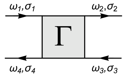
Figure 1: Vertex function $\Gamma_{\sigma_{1}\sigma_{2};\sigma_{3}\sigma_{4}}(i\omega_{1},i\omega_{2};i\omega_{3},i\omega_{4})$ satisfies the anti-symmetry property: Eq. (53) with $\omega_{1}+\omega_{3}=\omega_{2}+\omega_{4}$.

II.2 Non-linear susceptibilities: 3-body fluctuations

The next leading Fermi-liquid corrections are determined by the static nonlinear susceptibilities, as we will describe later,

$$\chi_{\sigma_{1}\sigma_{2}\sigma_{3}}^{[3]}\equiv\ -\,\frac{\partial^{3}\Omega}{\partial\epsilon_{d\sigma_{1}}\partial\epsilon_{d\sigma_{2}}\partial\epsilon_{d\sigma_{3}}}\,=\,\frac{\partial\chi_{\sigma_{2}\sigma_{3}}}{\partial\epsilon_{d\sigma_{1}}}.$$ (16)

It also corresponds to the thee-body correlations of the impurity occupation

$$\chi_{\sigma_{1}\sigma_{2}\sigma_{3}}^{[3]}\!=-\!\int_{0}^{\beta}\!\!\!d\tau_{3}\!\!\int_{0}^{\beta}\!\!\!d\tau_{2}\,\langle T_{\tau}\delta n_{d\sigma_{3}}(\tau_{3})\,\delta n_{d\sigma_{2}}(\tau_{2})\,\delta n_{d\sigma_{1}}\rangle.$$ (17)

We have provided a derivation of the nonlinear response function in Appendix A. More generally, the $n$-th derivative of $\Omega$ for $n=4,5,6\cdots$ corresponds to the $n$-body correlation function $\chi_{\sigma_{1}\sigma_{2}\sigma_{3}\cdots}^{[n]}$. The Fermi-liquid corrections can be classified according to $n$, and the derivative of the Ward identity reveals a hierarchy of Fermi-liquid relations, as described below. The $n$-body correlation function has permutation symmetry for the spin indexes $\chi_{\sigma_{1}\sigma_{2}\sigma_{3}\cdots}^{[n]}=\chi_{\sigma_{2}\sigma_{1}\sigma_{3}\cdots}^{[n]}=\chi_{\sigma_{3}\sigma_{2}\sigma_{1}\cdots}^{[n]}=\cdots$, and thus it has $n+1$ independent components at finite magnetic fields. Thus, for the three-body functions $3$ components among $2^{3}$ are independent at finite magnetic fields: for instance, the following for $\sigma=\uparrow,\downarrow$,

$$\frac{\partial\chi_{\sigma\sigma}}{\partial\epsilon_{d\sigma}}=\frac{\partial\chi_{\sigma\sigma}}{\partial\epsilon_{d}}-\frac{\partial\chi_{\uparrow\downarrow}}{\partial\epsilon_{d\sigma}},\quad\ \frac{\partial\chi_{\uparrow\downarrow}}{\partial\epsilon_{d\sigma}}=\frac{1}{2}\left(\frac{\partial\chi_{\uparrow\downarrow}}{\partial\epsilon_{d}}-\sigma\frac{\partial\chi_{\uparrow\downarrow}}{\partial h}\right).$$ (18)

Note that $\chi_{\uparrow\downarrow}$ is an even function of $h$, and thus $\partial\chi_{\uparrow\downarrow}/\partial h\xrightarrow{\,h\to 0\,}0$. The derivative of the renormalization factor $\widetilde{\chi}_{\sigma\sigma^{\prime}}$ also has a similar permutation symmetry but in a constrained way,

$$\frac{\partial^{2}\Sigma_{\sigma}(0)}{\partial\epsilon_{d\sigma_{2}}\partial\epsilon_{d\sigma_{1}}}\,= \ \frac{\partial\widetilde{\chi}_{\sigma\sigma_{1}}}{\partial\epsilon_{d\sigma_{2}}}\,=\,\frac{\partial\widetilde{\chi}_{\sigma\sigma_{2}}}{\partial\epsilon_{d\sigma_{1}}}$$ (19)

namely, the spin index $\sigma$ that corresponds to the index for the self-energy can not generally be exchanged with other indexes. It can explicitly be expressed, using the derivative of the susceptibilities, as

$$\frac{\partial\widetilde{\chi}_{\sigma_{1}\sigma_{2}}}{\partial\epsilon_{d\sigma_{3}}}\,=\,\frac{1}{\rho_{d\sigma_{1}}}\left(\frac{\partial\chi_{\sigma_{1}\sigma_{2}}}{\partial\epsilon_{d\sigma_{3}}}\,+\,2\pi\,\cot\delta_{\sigma_{1}}\,\chi_{\sigma_{1}\sigma_{3}}\chi_{\sigma_{1}\sigma_{2}}\right),$$ (20)

$$\ \frac{\partial}{\partial\epsilon_{d\sigma^{\prime}}}\left(\frac{1}{\rho_{d\sigma}}\right)\,=\,2\pi\cot\delta_{\sigma}\,\widetilde{\chi}_{\sigma\sigma^{\prime}}\,.$$ (21)

We also note that the correspondence between the above parameters and the coefficients used in FMvDM’s phenomenological description can be listed as

$$\frac{\alpha_{1\sigma}}{\pi}\,= \ \chi_{\sigma\sigma}\,,\qquad\qquad\frac{\phi_{1}}{\pi}\,=\,-\chi_{\uparrow\downarrow}\,,$$ (22)

$$\frac{\alpha_{2\sigma}}{\pi}= \ -\frac{1}{2}\,\frac{\partial\chi_{\sigma\sigma}}{\partial\epsilon_{d\sigma}},\qquad\frac{\phi_{2\sigma}}{\pi}=2\,\frac{\partial\chi_{\uparrow\downarrow}}{\partial\epsilon_{d\sigma}}\;.$$ (23)

II.3 Example: $T^{2}$ correction of electric resistance

Before going into details, we would like to show an example of how the non-linear susceptibilities $\chi_{\sigma_{1}\sigma_{2}\sigma_{3}}^{[3]}$ enter the Fermi-liquid corrections. Specifically, we consider the electric resistance $R_{\mathrm{MA}}$ of a dilute magnetic alloy (MA),

$$\frac{1}{R_{\mathrm{MA}}}= \ \frac{1}{2R_{\mathrm{MA}}^{0}}\sum_{\sigma}\mathcal{L}_{0,\sigma}\,,$$ (24)

$$\mathcal{L}_{0,\sigma}=\int_{-\infty}^{\infty}d\omega\,\frac{1}{\pi\Delta\rho_{d\sigma}(\omega,T)}\left(-\frac{\partial f(\omega)}{\partial\omega}\right).$$ (25)

Here, $R_{\mathrm{MA}}^{0}$ is the unitary-limit value of the electric resistance, and $f(\omega)=[e^{\beta\omega}+1]^{-1}$ is the Fermi function. Calculating the density of states $\rho_{d\sigma}(\omega,T)$ up to terms of order $\omega^{2}$ and $T^{2}$ with the self-energy presented in Eqs. (63) and (64), $\mathcal{L}_{0,\sigma}$ can be deduced up to order $T^{2}$,

$$\mathcal{L}_{0,\sigma}= \ \frac{1}{\pi\Delta\rho_{d\sigma}}\left[\,1+\frac{C_{0,\sigma}^{\mathrm{MA}}}{\pi\Delta\rho_{d\sigma}}\left(\pi T\right)^{2}\,\right]\,+O(T^{4}),$$ (26)

$$C_{0,\sigma}^{\mathrm{MA}}= \ \frac{\pi^{2}}{3}\Biggl{[}\,\bigl{(}2+\cos 2\delta_{\sigma}\bigr{)}\,\chi_{\sigma\sigma}^{2}-2\cos 2\delta_{\sigma}\,\chi_{\uparrow\downarrow}^{2}$$

$$\qquad+\frac{\sin 2\delta_{\sigma}}{2\pi}\,\left(\frac{\partial\chi_{\sigma\sigma}}{\partial\epsilon_{d\sigma}}+\frac{\partial\chi_{\uparrow\downarrow}}{\partial\epsilon_{d,-\sigma}}\right)\,\Biggr{]}\;.$$ (27)

We see that additional contributions of three-body fluctuations emerge in the coefficient $C_{0,\sigma}^{\mathrm{MA}}$ away from half-filling through the derivative of the linear susceptibilities. They vanish in the particle-hole symmetric case where $\epsilon_{d\sigma}=-U/2$, $h=0$, and the phase shift takes the unitary-limit value $\delta_{\sigma}=\pi/2$: then the coefficient is given by Yamada-Yosida’s formula,Yamada (1975a, b)

$$C_{0,\sigma}^{\mathrm{MA}}\longrightarrow\frac{\pi^{2}}{3}\Bigl{(}\chi_{\uparrow\uparrow}^{2}+2\chi_{\uparrow\downarrow}^{2}\Bigr{)}\,.$$ (28)

III Hierarchy of Fermi-liquid relations

In this section, we describe how a series of the Fermi-liquid relations can be derived from the Ward identity which reflects the local current conservation of each spin component $\sigma$,Yamada (1975a); Yoshimori (1976)

$$-\delta_{\sigma\sigma^{\prime}}\frac{\partial\Sigma_{\sigma}(i\omega)}{\partial i\omega}\,=\,\frac{\partial\Sigma_{\sigma}(i\omega)}{\partial\epsilon_{d\sigma^{\prime}}}+\Gamma_{\sigma\sigma^{\prime};\sigma^{\prime}\sigma}(i\omega,0;0,i\omega)\,\rho_{d\sigma^{\prime}}.$$ (29)

Here, $\Gamma_{\sigma_{2}\sigma_{3};\sigma_{4}\sigma_{4}}(i\omega_{1},i\omega_{2};i\omega_{3},i\omega_{4})$ is the four-point vertex function, the frequencies and suffixes of which are assigned in such a way shown in Fig. 1: some examples of the lowest-order diagrams are also shown in Figs.  2 and 3. The Ward identity describes a relation between the vertex function and the differential coefficients of the self-energy.

III.1 Leading Fermi-liquid corrections and the higher hierarchies

The Ward identity for $\omega=0$ is also called the Fermi-liquid relation. Specifically, the anti-parallel $\sigma^{\prime}=-\sigma$ and parallel $\sigma^{\prime}=\sigma$ spin components of Eq. (29) can be expressed in the following forms,Yamada (1975a); Yoshimori (1976) respectively,

$$\Gamma_{\sigma,-\sigma;-\sigma\sigma}(0,0;0,0)\,\rho_{d,-\sigma}=-\widetilde{\chi}_{\sigma,-\sigma},\qquad\frac{1}{z_{\sigma}}=\widetilde{\chi}_{\sigma\sigma}.$$ (30)

Note that $\Gamma_{\sigma\sigma;\sigma\sigma}(0,0;0,0)=0$ due to the Pauli exclusion rule, and $\Gamma_{\uparrow\downarrow;\downarrow\uparrow}(0,0;0,0)=\Gamma_{\downarrow\uparrow;\uparrow\downarrow}(0,0;0,0)$. Reflecting the property $1/z_{\sigma}=\widetilde{\chi}_{\sigma\sigma}$, the frequency derivative and the $\epsilon_{d\sigma}$ derivative of the density of states are identical except for the sign,

$$\rho_{d\sigma}^{\prime}\equiv\left.\frac{\partial\rho_{d\sigma}(\epsilon)}{\partial\epsilon}\right|_{\epsilon=0}=-\frac{\partial\rho_{d\sigma}}{\partial\epsilon_{d\sigma}}.$$ (31)

The leading Fermi-liquid corrections are characterized by the parameters $\widetilde{\chi}_{\sigma\sigma}$ and $\widetilde{\chi}_{\sigma,-\sigma}$, i.e., the first derivatives of the self-energy. For instance, Eq. (7) means that the susceptibilities are enhanced from the one for the free quasi-particles $\rho_{d\sigma}$ by the factor $\widetilde{\chi}_{\sigma\sigma^{\prime}}$. Furthermore, as a first step, the low-frequency expansion of the self-energy up to the $\omega$-linear terms is given in terms of the phase shift and the renormalization factor,

$$\epsilon_{d\sigma}+\Sigma_{\sigma}(i\omega)\,=\,\Delta\,\cot\delta_{\sigma}+\bigl{(}1-\widetilde{\chi}_{\sigma\sigma}\bigr{)}\,i\omega+O(\omega^{2}).$$ (32)

A series of the Fermi-liquid relations can be deduced, step by step, from the higher-order derivatives of the Ward identity for $n=1,2,3,\ldots$,

$$-\delta_{\sigma\sigma^{\prime}}\,\frac{\partial^{n+1}\Sigma_{\sigma}(i\omega)}{\partial(i\omega)^{n+1}}\ =\ \frac{\partial}{\partial\epsilon_{d\sigma^{\prime}}}\left(\frac{\partial^{n}\Sigma_{\sigma}(i\omega)}{\partial(i\omega)^{n}}\right)+\frac{\partial^{n}}{\partial(i\omega)^{n}}\Gamma_{\sigma\sigma^{\prime};\sigma^{\prime}\sigma}(i\omega,0;0,i\omega)\,\rho_{d\sigma^{\prime}}.$$ (33)

Here, for the first term on the right-hand side, the derivative with respect to $i\omega$ and that with respect to $\epsilon_{d\sigma^{\prime}}$ have been commuted. Equation (33) means that the $n+1$-th derivative of $\Sigma_{\sigma}(i\omega)$ in the left-hand side will be calculated from the $n$-th one if the additional vertex term for the parallel spins

$$\frac{\partial^{n}}{\partial(i\omega)^{n}}\Gamma_{\sigma\sigma;\sigma\sigma}(i\omega,0;0,i\omega)$$ (34)

is explicitly known. Therefore, the derivative of $\Gamma_{\sigma\sigma;\sigma\sigma}(i\omega,0;0,i\omega)$ plays a central role to proceed iteratively to the next step. The Fermi-liquid relations of the $n+1$-th step can be written in the following form, for the anti-parallel $\sigma^{\prime}=-\sigma$ and the parallel $\sigma^{\prime}=\sigma$ spin components of Eq. (33), respectively,

$$\ \ \left.\frac{\partial^{n}}{\partial(i\omega)^{n}}\Gamma_{\sigma,-\sigma;-\sigma,\sigma}(i\omega,0;0,i\omega)\,\rho_{d,-\sigma}\right|_{\omega\to 0}\ =\ \ \left.-\frac{\partial}{\partial\epsilon_{d,-\sigma}}\left(\frac{\partial^{n}\Sigma_{\sigma}(i\omega)}{\partial(i\omega)^{n}}\right)\right|_{\omega\to 0},$$ (35)

$$\left.-\frac{\partial^{n+1}\Sigma_{\sigma}(i\omega)}{\partial(i\omega)^{n+1}}\right|_{\omega\to 0}=\ (-1)^{n}\frac{\partial^{n+1}\Sigma_{\sigma}(0)}{\partial\epsilon_{d\sigma}^{n+1}}\ \ +\ \ \sum_{k=1}^{n-1}(-1)^{k}\!\!\left.\frac{\partial^{k}}{\partial\epsilon_{d\sigma}^{k}}\left(\frac{\partial^{n-k}}{\partial(i\omega)^{n-k}}\Gamma_{\sigma\sigma;\sigma\sigma}(i\omega,0;0,i\omega)\,\rho_{d\sigma}\,\right)\right|_{\omega\to 0}$$

$$\qquad\qquad\qquad\qquad\quad\ \ +\left.\frac{\partial^{n}}{\partial(i\omega)^{n}}\Gamma_{\sigma\sigma;\sigma\sigma}(i\omega,0;0,i\omega)\,\rho_{d\sigma}\right|_{\omega\to 0}.$$ (36)

The first term in the right-hand side of Eq. (36) corresponds to the $n$-th derivative of $\widetilde{\chi}_{\sigma\sigma}$ with respect to $\epsilon_{d\sigma}$, and can be related to the ($n+2$)-body correlation function $\chi_{\sigma\sigma\sigma\ldots}^{[n+2]}$, which correspond to a generalization of Eqs. (16) and (17). Therefore, the ($n+1$)-th step Fermi-liquid relations are determined by the static nonlinear susceptibilities of $\delta n_{d\sigma}$ up to the ($n+2$)-th order.

   

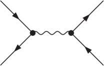
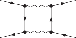
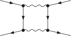
Figure 2: Order $U$ and $U^{2}$ vertex function $\Gamma_{\sigma,-\sigma;-\sigma,\sigma}$: the anti-parallel spin component.

 

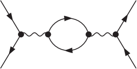
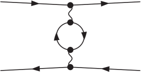
Figure 3: Order $U^{2}$ vertex function $\Gamma_{\sigma\sigma;\sigma\sigma}$: the parallel spin component.

   

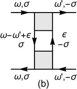
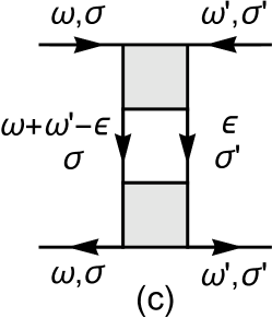
Figure 4: Feynman diagrams, which cause the singularities of the vertex function $\Gamma_{\sigma\sigma^{\prime};\sigma^{\prime}\sigma}(i\omega,i\omega^{\prime};i\omega^{\prime},i\omega)$ for small $\omega$ and $\omega^{\prime}$. The intermediate particle-hole excitation in (a) and (b) yields the non-analytic $\mathrm{sgn}\,(\omega-\omega^{\prime})$ term. The particle-particle excitation in (c) yields the $\mathrm{sgn}\,(\omega+\omega^{\prime})$ term. As the vertex function, which is represented by the shaded square, vanishes $\Gamma_{\sigma\sigma;\sigma\sigma}(0,0;0,0)=0$ for parallel spins at zero frequencies, the non-analytic terms emerge for the spin configurations of (a) $\sigma^{\prime\prime}=-\sigma$, (b) $\sigma=\uparrow,\downarrow$, and (c) $\sigma^{\prime}=-\sigma$.

III.2 Next-leading Fermi-liquid corrections: the $n=1$ hierarchy

The next leading (2nd step) Fermi-liquid relations are generated from the first derivative of the Ward identity, namely Eqs. (35) and (36) for $n=1$:

$$\left.\frac{\partial}{\partial i\omega}\Gamma_{\sigma,-\sigma;-\sigma\sigma}(i\omega,0;0,i\omega)\,\rho_{d,-\sigma}\right|_{\omega\to 0}$$

$$= \ \ \frac{\partial}{\partial\epsilon_{d,-\sigma}}\left(\frac{\partial\Sigma_{\sigma}(0)}{\partial\epsilon_{d\sigma}}\right),$$ (37)

$$\left.\frac{\partial^{2}\Sigma_{\sigma}(i\omega)}{\partial(i\omega)^{2}}\right|_{\omega\to 0}$$

$$= \ \frac{\partial}{\partial\epsilon_{d\sigma}}\left(\frac{\partial\Sigma_{\sigma}(0)}{\partial\epsilon_{d\sigma}}\right)-\left.\frac{\partial}{\partial i\omega}\Gamma_{\sigma\sigma;\sigma\sigma}(i\omega,0;0,i\omega)\,\rho_{d\sigma}\right|_{\omega\to 0}.$$ (38)

For the second derivative of the self-energy on the right-hand side of these two equations, we have used the relation $1/z_{\sigma}=\widetilde{\chi}_{\sigma\sigma}$ given in Eq.  (30). These two terms can also be written in terms of the first derivative of $\widetilde{\chi}_{\sigma\sigma}$ with respect to $\epsilon_{d\sigma^{\prime}}$, and are related to the three-body correlation function $\chi_{\sigma\sigma\sigma^{\prime}}^{[3]}$.

From Eqs. (30) and (37), the vertex function for anti-parallel spins $\Gamma_{\sigma,-\sigma;-\sigma\sigma}(i\omega,0;0,i\omega)$ can be deduced up to the $\omega$-linear term,

$$\Gamma_{\sigma,-\sigma;-\sigma\sigma}(i\omega,0;0,i\omega)\,\rho_{d,-\sigma}$$

$$\qquad\qquad\quad=\ -\widetilde{\chi}_{\sigma,-\sigma}+\frac{\partial\widetilde{\chi}_{\sigma,-\sigma}}{\partial\epsilon_{d\sigma}}\,i\omega+O(\omega^{2}).$$ (39)

It shows that the $\omega$-linear term does not accompany a singular $\omega\,\mathrm{sgn}(\omega)$ dependence which converts into the imaginary part by the analytic continuation $i\omega\to\omega+i0^{+}$.Yamada (1975b); Shiba (1975) This has been perturbatively understood as follows. For the anti-parallel spins vertex, the non-analytic $\omega\,\mathrm{sgn}(\omega)$ dependence disappears as a result of the cancellation between the contribution of the particle-hole pair and that of the particle-particle pair. These pairs first emerge in the order $U^{2}$ processes described in Fig. 2, where the particle and hole carry different spins, $\sigma$ and $-\sigma$. The total contributions, which include all the higher-order processes described in Fig. 4 (b) and (c) for $\sigma^{\prime}=-\sigma$, cancel each other out: it can be confirmed explicitly through Eq. (62).

We next consider the relation for the parallel spin component given in Eq. (38). The first term in the right-hand side is real and is given by $\partial\widetilde{\chi}_{\sigma\sigma}/\partial\epsilon_{d\sigma}$. Therefore, the discontinuous $\mathrm{sgn}(\omega)$ dependence emerges only from the second term, namely first derivative of $\Gamma_{\sigma\sigma;\sigma\sigma}(i\omega,0;0,i\omega)$ with respect to $i\omega$. It was also shown by Yamada-Yosida that the discontinuous $\mathrm{sgn}(\omega)$ dependence in the derivative emerges from the intermediate one particle-hole pair carrying spin $-\sigma$, which is opposite to the spin $\sigma$ of the external line: diagrams for the order $U^{2}$ processes and for the generalized ones are shown in Figs.  3, 4 (a), and 4 (c) for $\sigma^{\prime}=\sigma$, respectively. The contribution has been obtained in the formYamada (1975b); Yoshimori (1976)

$$\mathrm{Im}\left.\frac{\partial}{\partial i\omega}\Gamma_{\sigma\sigma;\sigma\sigma}(i\omega,0;0,i\omega)\,\rho_{d\sigma}\right|_{\omega\to 0}=\,\pi\frac{\chi_{\uparrow\downarrow}^{2}}{\rho_{d\sigma}}\,\mathrm{sgn}(\omega)\;.$$ (40)

From this result and the relation Eq. (38), the $\omega^{2}$ imaginary part of the self-energy also has been deduced:Yamada (1975b); Yoshimori (1976)

$$\mathrm{Im}\left.\frac{\partial^{2}\Sigma_{\sigma}(i\omega)}{\partial(i\omega)^{2}}\,\right|_{\omega\to 0}=\,-\pi\,\frac{\chi_{\uparrow\downarrow}^{2}}{\rho_{d\sigma}}\,\mathrm{sgn}(\omega)\;.$$ (41)

In contrast to the non-analytic component, the analytic component of the $\omega$-linear part of $\Gamma_{\sigma\sigma;\sigma\sigma}(i\omega,0;0,i\omega)$ has not been studied in detail so far. This part will contribute to low-energy transport away from half-filling if it is finite. In the present paper we calculate the regular part using a Green’s-function product expansion, and show that it identically vanishes,

$$\mathrm{Re}\left.\frac{\partial}{\partial i\omega}\Gamma_{\sigma\sigma;\sigma\sigma}(i\omega,0;0,i\omega)\,\rho_{d\sigma}\right|_{\omega\to 0}=\,0\;.$$ (42)

This is one of the key features of the vertex function, and is caused by its anti-symmetry property. We provide a microscopic proof later in the present paper. An important identity, which relates the real parts of two different second derivatives of the self-energy, follows from Eqs. (38) and (42),

$$\mathrm{Re}\left.\frac{\partial^{2}\Sigma_{\sigma}(i\omega)}{\partial(i\omega)^{2}}\,\right|_{\omega\to 0}=\,\frac{\partial^{2}\Sigma_{\sigma}(0)}{\partial\epsilon_{d\sigma}^{2}}\;.$$ (43)

This relation agree with FMvDM’s formula given in Eq. (B8b) of Ref. Filippone et al., 2017, which was obtained by extending Nozières’ phenomenological description.

From the knowledge of Eqs.  (40) and (42), the low-frequency behavior of the parallel-spin component of the vertex function can be explicitly written up to the $\omega$-linear part:

$$\Gamma_{\sigma\sigma;\sigma\sigma}(i\omega,0;0,i\omega)\,\rho_{d\sigma}^{2}=\,i\pi\,\chi_{\uparrow\downarrow}^{2}\,i\omega\,\mathrm{sgn}(\omega)+O(\omega^{2}).$$ (44)

Note that the non-analytic $\omega$-linear term corresponds to the absolute value $|\omega|=\omega\,\mathrm{sgn}(\omega)$, which has a cusp at $\omega=0$. Then, using Eqs. (41) and (43) with Eq. (19), the self-energy can be determined up to the $(i\omega)^{2}$ term which extends Eq. (32), as

$$\epsilon_{d\sigma}+\Sigma_{\sigma}(i\omega)= \ \Delta\,\cot\delta_{\sigma}+\bigl{(}1-\widetilde{\chi}_{\sigma\sigma}\bigr{)}\,i\omega$$

$$\!\!\!\!\!\!\!\!\!\!\!\!\!\!+\frac{1}{2}\left(\frac{\partial\widetilde{\chi}_{\sigma\sigma}}{\partial\epsilon_{d\sigma}}-i\pi\frac{\chi_{\uparrow\downarrow}^{2}}{\rho_{d\sigma}}\,\mathrm{sgn}(\omega)\right)(i\omega)^{2}+O(\omega^{3}).$$ (45)

The next-leading Fermi-liquid correction that enters through ${\partial\widetilde{\chi}_{\sigma\sigma}}/{\partial\epsilon_{d\sigma^{\prime}}}$ vanishes in the particle-hole symmetric case at zero magnetic field. This is because the spin and charge susceptibilities take extreme values: ${\partial\chi_{s}}/{\partial\epsilon_{d}}=0$ and ${\partial\chi_{c}}/{\partial\epsilon_{d}}=0$, at $\xi_{d}\equiv\epsilon_{d}+U/2=0$ and $h=0$.

III.3 Higher-order Fermi-liquid corrections for $n=2$

We can also deduce the second derivative of the vertex function for the anti-parallel spins from Eqs. (40) and (43) through Eq. (35) for $n=2$,

$$\!\!\!\!\!\!\left.\frac{\partial^{2}}{\partial(i\omega)^{2}}\Gamma_{\sigma,-\sigma;-\sigma,\sigma}(i\omega,0;0,i\omega)\,\rho_{d,-\sigma}\right|_{\omega\to 0}$$

$$=\ -\,\frac{\partial}{\partial\epsilon_{d,-\sigma}}\left.\left(\frac{\partial^{2}\Sigma_{\sigma}(i\omega)}{\partial(i\omega)^{2}}\right)\right|_{\omega\to 0}$$

$$=\ \frac{\partial}{\partial\epsilon_{d,-\sigma}}\left(-\frac{\partial^{2}\Sigma_{\sigma}(0)}{\partial\epsilon_{d\sigma}^{2}}+i\pi\,\frac{\chi_{\uparrow\downarrow}^{2}}{\rho_{d\sigma}}\,\mathrm{sgn}(\omega)\right).$$ (46)

Therefore, adding the $\omega^{2}$ term to Eq. (39), we obtain the low-energy expansion in an extended form:

$$\!\!\Gamma_{\sigma,-\sigma;-\sigma,\sigma}(i\omega,0;0,i\omega)\,\rho_{d\sigma}\rho_{d,-\sigma}=\,-\chi_{\uparrow\downarrow}+\rho_{d\sigma}\frac{\partial\widetilde{\chi}_{\sigma,-\sigma}}{\partial\epsilon_{d\sigma}}\ i\omega+\frac{\rho_{d\sigma}}{2}\,\frac{\partial}{\partial\epsilon_{d,-\sigma}}\left[-\frac{\partial\widetilde{\chi}_{\sigma\sigma}}{\partial\epsilon_{d\sigma}}+i\pi\,\frac{\chi_{\uparrow\downarrow}^{2}}{\rho_{d\sigma}}\,\mathrm{sgn}(\omega)\right](i\omega)^{2}+\cdots$$ (47)

This is also one of the most important results of the present work. The $\omega^{2}$ term involves higher-order corrections which correspond to the static four-body susceptibilities $\chi_{\sigma\sigma\sigma,-\sigma}^{[4]}$. At zero field $h=0$, the coefficients for the imaginary and real part of the $\omega^{2}$ term can be expressed in the form of Eqs.  (128) and (132), given in Appendix C. Specifically in the particle-hole symmetric case at zero magnetic field,

$$\frac{\Gamma_{\sigma,-\sigma;-\sigma,\sigma}(i\omega,0;0,i\omega)}{\pi\Delta}$$

$$\qquad\quad=\ -\widetilde{\chi}_{\uparrow\downarrow}-\frac{1}{2}\left.\frac{\partial^{2}\widetilde{\chi}_{\sigma,-\sigma}}{\partial\epsilon_{d\sigma}^{2}}\right|_{h\to 0\atop\xi_{d}\to 0}(i\omega)^{2}+\cdots.$$ (48)

The real part of the $\omega^{2}$ term remains finite with the coefficient

$$\left.\frac{1}{\pi\Delta}\frac{\partial^{2}\widetilde{\chi}_{\sigma,-\sigma}}{\partial\epsilon_{d\sigma}^{2}}\right|_{h\to 0\atop\xi_{d}\to 0}$$

$$\qquad=\left.\frac{1}{4}\left(\frac{\partial^{2}\chi_{\uparrow\downarrow}}{\partial\epsilon_{d}^{2}}+\frac{\partial^{2}\chi_{\uparrow\downarrow}}{\partial h^{2}}\right)\right|_{h\to 0\atop\xi_{d}\to 0}\!\!+2\pi^{2}\chi_{\uparrow\downarrow}\chi_{\uparrow\uparrow}^{2}.$$ (49)

Fermi-liquid corrections of this order, $n=2$, also emerge in the order $\omega^{2}$ contributions of the parallel spins component. Therefore, to take into account all corrections of this order, one needs to calculate

$$\left.\frac{\partial^{2}}{\partial(i\omega)^{2}}\Gamma_{\sigma\sigma;\sigma\sigma}(i\omega,0;0,i\omega)\,\rho_{d\sigma}\right|_{\omega\to 0}\;.$$ (50)

Then, $\frac{\partial^{3}\Sigma_{\sigma}(i\omega)}{\partial(i\omega)^{3}}$ follows through Eq. (36) for $n=2$.

IV Double-frequency expansion of $\Gamma_{\sigma\sigma^{\prime};\sigma^{\prime}\sigma}(i\omega,i\omega^{\prime};i\omega^{\prime},i\omega)$

In this section, we show that the double-frequency expansion of $\Gamma_{\sigma\sigma^{\prime};\sigma^{\prime}\sigma}(i\omega,i\omega^{\prime};i\omega^{\prime},i\omega)$ up to the linear terms in $\omega$ and $\omega^{\prime}$ can also be expressed in terms of the Fermi-liquid parameters. The results are shown in Eqs. (51) and (52): for the parallel component $\sigma^{\prime}=\sigma$,

$$\Gamma_{\sigma\sigma;\sigma\sigma}(i\omega,i\omega^{\prime};i\omega^{\prime},i\omega)\,\rho_{d\sigma}^{2}\,=\,-\pi\,\chi_{\uparrow\downarrow}^{2}\left|\omega-\omega^{\prime}\right|+\cdots,$$ (51)

and for $\sigma^{\prime}=-\sigma$ it is

$$\Gamma_{\sigma,-\sigma;-\sigma,\sigma}(i\omega,i\omega^{\prime};i\omega^{\prime},i\omega)\,\rho_{d\sigma}\rho_{d,-\sigma}\,=\,\,-\chi_{\uparrow\downarrow}+\rho_{d\sigma}\frac{\partial\widetilde{\chi}_{\sigma,-\sigma}}{\partial\epsilon_{d\sigma}}\,i\omega+\rho_{d,-\sigma}\frac{\partial\widetilde{\chi}_{-\sigma,\sigma}}{\partial\epsilon_{d,-\sigma}}\,i\omega^{\prime}-\pi\,\chi_{\uparrow\downarrow}^{2}\Bigl{[}\,\left|\omega-\omega^{\prime}\right|-\left|\omega+\omega^{\prime}\right|\,\Bigr{]}+\cdots.$$ (52)

Note that $\left|\omega\pm\omega^{\prime}\right|=-i(i\omega\pm i\omega^{\prime})\ \mathrm{sgn}(\omega\pm\omega^{\prime})$.

These asymptotically exact results capture the essential features of the Fermi liquid, and are analogous to Landau’s quasi-particle interaction $f(\bm{p}\,\sigma,\bm{p}^{\prime}\sigma^{\prime})$ and Nozières’ function $\phi_{\sigma\sigma^{\prime}}(\varepsilon,\varepsilon^{\prime})$. Abrikosov et al. (1965); Nozières (1974) One important difference is that the vertex function also has a non-analytic part which directly determines the damping of the quasi-particles. We give the derivations of Eqs. (51) and (52) in the following.

 

Figure 5: Non-analytic $|\omega-\omega^{\prime}|$ and $|\omega+\omega^{\prime}|$ contributions of $\Gamma_{\sigma\sigma;\sigma\sigma}(i\omega,i\omega^{\prime};i\omega^{\prime},i\omega)$ and $\Gamma_{\sigma,-\sigma;-\sigma,\sigma}(i\omega,i\omega^{\prime};i\omega^{\prime},i\omega)$.

IV.1 Anti-symmetry properties of $\Gamma_{\sigma\sigma^{\prime};\sigma^{\prime}\sigma}(i\omega,i\omega^{\prime};i\omega^{\prime},i\omega)$

Two important features of the vertex function, the anti-symmetric property and analytic property, play an essential role in the proof, which we provide in this section. The fermionic antisymmetric commutation relation imposes a strong restriction on the vertex function,

$$\!\!\!\!\!\!\!\!\!\!\!\!\!\!\!\!\!\!\!\!\!\!\!\!\!\!\!\!\!\!\!\Gamma_{\sigma_{1}\sigma_{2};\sigma_{3}\sigma_{4}}(i\omega_{1},i\omega_{2};i\omega_{3},i\omega_{4})$$

$$= \ \ \Gamma_{\sigma_{3}\sigma_{4};\sigma_{1}\sigma_{2}}(i\omega_{3},i\omega_{4};i\omega_{1},i\omega_{2})$$

$$= \,-\Gamma_{\sigma_{3}\sigma_{2};\sigma_{1}\sigma_{4}}(i\omega_{3},i\omega_{2};i\omega_{1},i\omega_{4})$$

$$= \,-\Gamma_{\sigma_{1}\sigma_{4};\sigma_{3}\sigma_{2}}(i\omega_{1},i\omega_{4};i\omega_{3},i\omega_{2}).$$ (53)

Obviously, $\Gamma_{\sigma\sigma;\sigma\sigma}(0,0;0,0)=0$ follows from Eq. (53) at zero frequencies. The anti-symmetry property also imposes strong constrains in the linear $\omega$ and $\omega^{\prime}$ dependences. The analytic properties of the vertex function is another key to determine the explicit form of the linear terms. The vertex function $\Gamma_{\sigma\sigma^{\prime};\sigma^{\prime}\sigma}(i\omega,i\omega^{\prime};i\omega^{\prime},i\omega)$ has some singularities in the $\omega$-$\omega^{\prime}$ plane.Eliashberg (1962a, b) Specifically, the non-analytic terms emerge through the three diagrams given in Fig. 4 for small $\omega$ and $\omega^{\prime}$. The intermediate particle-hole and particle-particle pair excitations in the Anderson impurity yield the non-analytic terms of the form $|\omega-\omega^{\prime}|$ and $|\omega+\omega^{\prime}|$, respectively, which divide the $\omega$-$\omega^{\prime}$ plane as shown in Fig. 5. Thus, the linear terms of the double-frequency expansion can be expressed as a linear combination of $\omega$, $\omega^{\prime}$, $|\omega-\omega^{\prime}|$, and $|\omega+\omega^{\prime}|$;

$$\Gamma_{\sigma\sigma;\sigma\sigma}(i\omega,i\omega^{\prime};i\omega^{\prime},i\omega)\,\rho_{d\sigma}^{2}$$

$$\quad=\,a_{\sigma\sigma}\bigl{(}i\omega+i\omega^{\prime}\bigr{)}+b_{\sigma\sigma}^{-}\,|\omega-\omega^{\prime}|+b_{\sigma\sigma}^{+}\,|\omega+\omega^{\prime}|+\cdots$$ (54)

$$\Gamma_{\sigma,-\sigma;-\sigma,\sigma}(i\omega,i\omega^{\prime};i\omega^{\prime},i\omega)\,\rho_{d\sigma}\rho_{d,-\sigma}$$

$$\quad=\,-\chi_{\uparrow\downarrow}+a_{\sigma,-\sigma}\,i\omega+a_{-\sigma,\sigma}\,i\omega^{\prime}+b_{\uparrow\downarrow}^{-}\,|\omega-\omega^{\prime}|$$

$$\quad\quad\ +b_{\uparrow\downarrow}^{+}\,|\omega+\omega^{\prime}|+\cdots.$$ (55)

Here, $a_{\sigma\sigma^{\prime}}$ and $b_{\sigma\sigma^{\prime}}^{\pm}$ with $b_{\uparrow\downarrow}^{\pm}=b_{\downarrow\uparrow}^{\pm}$ are the expansion coefficients for the analytic and non-analytic terms, respectively. Equations (54) and (55) are constructed in such way that each satisfies one of the requirements $\Gamma_{\sigma\sigma^{\prime};\sigma^{\prime}\sigma}(i\omega,i\omega^{\prime};i\omega^{\prime},i\omega)=\Gamma_{\sigma^{\prime}\sigma;\sigma\sigma^{\prime}}(i\omega^{\prime},i\omega;i\omega,i\omega^{\prime})$. In order to satisfy the remaining requirements of the anti-symmetry given in Eq. (53), the coefficient $a_{\sigma\sigma}$ for the parallel spin components must vanish as shown in Appendix B,

$$a_{\sigma\sigma}\,\equiv\,0\;.$$ (56)

Thus, the parallel-spin vertex does not have the analytic term. Equation (42) follows from this result. Therefore, as Eq. (47) has been deduced from Eq. (42) and the Ward identities, we can use Eq. (47) to determine $a_{\sigma,-\sigma}$ taking $\omega^{\prime}=0$,

$$a_{\sigma,-\sigma}\,\equiv\,\rho_{d\sigma}\frac{\partial\widetilde{\chi}_{\sigma,-\sigma}}{\partial\epsilon_{d\sigma}}\;.$$ (57)

IV.2 Non-analytic part of $\Gamma_{\sigma\sigma^{\prime};\sigma^{\prime}\sigma}(i\omega,i\omega^{\prime};i\omega^{\prime},i\omega)$ for small $\omega$ and $\omega^{\prime}$

In the following, we calculate the non-analytic part of $\Gamma_{\sigma\sigma^{\prime};\sigma^{\prime}\sigma}(i\omega,i\omega^{\prime};i\omega^{\prime},i\omega)$, and directly derive the $|\omega-\omega^{\prime}|$ and $|\omega+\omega^{\prime}|$ contributions including the coefficients. The analytic and non-analytic parts of the first derivative of the vertex function with respect to $i\omega$, or $i\omega^{\prime}$, take real and pure-imaginary values, respectively. Specifically, we consider the imaginary part of the first derivative with respect to $i\omega^{\prime}$ in detail.

For the parallel spin vertex, the non-analytic term emerges from the diagram of Fig. 4 (a). For small $\omega$ and $\omega^{\prime}$, it is given by

$$\!\!\mathrm{Im}\,\rho_{d\sigma}\,\frac{\partial}{\partial i\omega^{\prime}}\,\Gamma_{\sigma\sigma;\sigma\sigma}(i\omega,i\omega^{\prime};i\omega^{\prime},i\omega)$$

$$=-\,\left|\Gamma_{\uparrow\downarrow;\downarrow\uparrow}(0,0;0,0)\right|^{2}$$

$$\quad\times\rho_{d\sigma}\,\mathrm{Im}\int\frac{d\varepsilon}{2\pi}\,G_{-\sigma}(i\varepsilon)\,\frac{\partial}{\partial i\omega^{\prime}}\,G_{-\sigma}(i\omega-i\omega^{\prime}+i\varepsilon)$$

$$=\,-\,\pi\left|\Gamma_{\uparrow\downarrow;\downarrow\uparrow}(0,0;0,0)\right|^{2}\,\rho_{d\sigma}\,\rho_{d,-\sigma}^{2}\ \mbox{sgn}(\omega-\omega^{\prime})\,.$$ (58)

Here, we have used the differential formula for the Green’s function, given in Eq. (75). The non-analytic terms of the anti-parallel spin vertex function emerge from the other two diagrams shown in Figs. 4 (b) and (c):

$$\!\!\mathrm{Im}\,\rho_{d,-\sigma}\,\frac{\partial}{\partial i\omega^{\prime}}\,\Gamma_{\sigma,-\sigma;-\sigma,\sigma}(i\omega,i\omega^{\prime};i\omega^{\prime},i\omega)$$

$$=-\,\left|\Gamma_{\uparrow\downarrow;\downarrow\uparrow}(0,0;0,0)\right|^{2}$$

$$\quad\times\rho_{d,-\sigma}\,\mathrm{Im}\Biggl{[}\int\frac{d\varepsilon}{2\pi}\,G_{-\sigma}(i\varepsilon)\,\frac{\partial}{\partial i\omega^{\prime}}\,G_{\sigma}(i\omega-i\omega^{\prime}+i\varepsilon)$$

$$\qquad\qquad\quad+\int\frac{d\varepsilon}{2\pi}\,G_{-\sigma}(i\varepsilon)\,\frac{\partial}{\partial i\omega^{\prime}}\,G_{\sigma}(i\omega+i\omega^{\prime}-i\varepsilon)\,\,\Biggr{]}$$

$$=\,-\,\pi\left|\Gamma_{\uparrow\downarrow;\downarrow\uparrow}(0,0;0,0)\right|^{2}\,$$

$$\qquad\times\rho_{d\sigma}\,\rho_{d,-\sigma}^{2}\Bigl{[}\,\,\mbox{sgn}(\omega-\omega^{\prime})\,+\,\,\mbox{sgn}(\omega+\omega^{\prime})\,\Bigr{]}.$$ (59)

Equations (58) and (59) determine the non-analytic $|\omega-\omega^{\prime}|$ and $|\omega+\omega^{\prime}|$ terms of $\Gamma_{\sigma\sigma^{\prime};\sigma^{\prime}\sigma}(i\omega,i\omega^{\prime};i\omega^{\prime},i\omega)$:

$$b_{\sigma\sigma}^{-}=b_{\uparrow\downarrow}^{-}=-b_{\uparrow\downarrow}^{+}=-\pi\chi_{\uparrow\downarrow}^{2},\qquad b_{\sigma\sigma}^{+}\,=\,0,$$ (60)

and we obtain Eqs.  (54) and (55). These non-analytic contributions divide the $\omega$-$\omega^{\prime}$ plane of $\Gamma_{\sigma\sigma^{\prime};\sigma^{\prime}\sigma}(i\omega,i\omega^{\prime};i\omega^{\prime},i\omega)$ into the separate analytic regions as in Fig. 5. Furthermore, from Eqs. (58) and (59), the single-frequency results described in Eqs. (39) and (40), which correspond to the result of Yamada-Yosida,Yamada (1975b) can be deduced, using $\Gamma_{\sigma\sigma^{\prime};\sigma^{\prime}\sigma}(i\omega,i\omega^{\prime};i\omega^{\prime},i\omega)=\Gamma_{\sigma^{\prime}\sigma;\sigma\sigma^{\prime}}(i\omega^{\prime},i\omega;i\omega,i\omega^{\prime})$:

$$\left.\mathrm{Im}\,\frac{\partial}{\partial i\omega}\Gamma_{\sigma\sigma;\sigma\sigma}(i\omega,0;0,i\omega)\,\rho_{d\sigma}\right|_{\omega\to 0}=\,\pi\,\frac{\chi_{\uparrow\downarrow}^{2}}{\rho_{d\sigma}}\,\mbox{sgn}(\omega),$$ (61)

$$\left.\mathrm{Im}\,\frac{\partial}{\partial i\omega}\Gamma_{\sigma,-\sigma;-\sigma,\sigma}(i\omega,0;0,i\omega)\,\rho_{d,-\sigma}\,\right|_{\omega\to 0}=\,0.$$ (62)

V The $T^{2}$ real part of self-energy

We next consider the $T^{2}$ correction of the retarded self-energy $\Sigma^{r}(\omega)$, especially the real part. Before describing the derivation, we show the result first. Including the $T^{2}$ correction, the low-energy asymptotic form of the self-energy can be expressed in the following form. The imaginary part is given by

$$\mathrm{Im}\,\Sigma_{\sigma}^{r}(\omega)\,=\,-\,\frac{\pi}{2}\,\frac{\chi_{\uparrow\downarrow}^{2}}{\rho_{d\sigma}}\,\Bigl{[}\,\omega^{2}+(\pi T)^{2}\,\Bigr{]}+\cdots,$$ (63)

and the real part is

$$\epsilon_{d\sigma}+\mathrm{Re}\,\Sigma_{\sigma}^{r}(\omega)\,=\,\Delta\,\cot\delta_{\sigma}\,+\bigl{(}1-\widetilde{\chi}_{\sigma\sigma}\bigr{)}\,\omega$$

$$\qquad\ \ +\frac{1}{2}\,\frac{\partial\widetilde{\chi}_{\sigma\sigma}}{\partial\epsilon_{d\sigma}}\,\omega^{2}+\frac{1}{6}\,\frac{1}{\rho_{d\sigma}}\frac{\partial\chi_{\uparrow\downarrow}}{\partial\epsilon_{d,-\sigma}}\,\left(\pi T\right)^{2}+\cdots.$$ (64)

At zero magnetic field $h=0$, the 3-body correlations can be rewritten in terms of the derivative with respect to the spin-independent impurity level $\epsilon_{d}$,

$$\epsilon_{d\sigma}+\mathrm{Re}\,\Sigma_{\sigma}^{r}(\omega)\ \xrightarrow{\,h\to 0\,}\ \ \Delta\,\cot\delta_{\sigma}\,+\bigl{(}1-\widetilde{\chi}_{\uparrow\uparrow}\bigr{)}\,\omega$$

$$\qquad\qquad+\frac{1}{2\rho_{d}}\left(\frac{\partial\chi_{\uparrow\uparrow}}{\partial\epsilon_{d}}-\frac{1}{2}\frac{\partial\chi_{\uparrow\downarrow}}{\partial\epsilon_{d}}+2\pi\cot\delta\ \chi_{\uparrow\uparrow}^{2}\right)\,\omega^{2}$$

$$\qquad\qquad+\frac{1}{12}\,\frac{1}{\rho_{d}}\frac{\partial\chi_{\uparrow\downarrow}}{\partial\epsilon_{d}}\,\left(\pi T\right)^{2}+\cdots\;.$$ (65)

V.1 Ward identity for the $T^{2}$ corrections

We calculate the finite-temperature $T^{2}$ correction of the self-energy using the Euler-Maclaurin formula

$$\sum_{n=0}^{\infty}q\Big{(}n+\frac{1}{2}\Bigr{)}\,\simeq\int_{0}^{\infty}\!dx\,q(x)+\frac{1}{24}\left.\frac{dq(x)}{dx}\right|_{x\to 0}.$$ (66)

Specifically, summation over the Matsubara frequency $\omega_{n}=(2n+1)\pi T$ of a function $\mathcal{Q}(i\omega_{n})$, which has a discontinuity at $\omega\to 0$, can be calculated by using the formula separately for $\omega_{n}>0$ and $\omega_{n}<0$, following Yamada-Yosida,Yamada (1975b)

$$T\!\sum_{n=-\infty}^{\infty}\mathcal{Q}(i\omega_{n})-\int_{-\infty}^{\infty}\!\frac{d\omega}{2\pi}\ \mathcal{Q}(i\omega)\,$$

$$=\ \frac{(\pi T)^{2}}{6}\left(\lim_{\omega\to 0^{+}}-\lim_{\omega\to 0^{-}}\right)\left(\frac{-1}{2\pi i}\frac{\partial\mathcal{Q}(i\omega)}{\partial i\omega}\right)+O(T^{4}).$$ (67)

The leading correction for the self-energy $\Sigma_{\sigma}(i\omega,T)$ of order $T^{2}$ is obtained by taking a functional derivative of the self-energy with respect to the full interacting Green’s function as shown in Sec. 19.5 of the book of Abrikosov, Gorkov and Dzyashinski (AGD), specifically the formula for order $T^{2}$ correction is given in Eq. (19.22) of AGD.Abrikosov et al. (1965) It can be derived by using the Luttinger-Ward functional,Luttinger and Ward (1960) and taking into account the corrections emerging through the summation over the Matsubara frequency and that through the other $T$-dependent part of the interacting $G_{\sigma}(i\omega_{n},T)$, where the second argument represents the temperature dependence emerging through the summation over the internal Matsubara frequencies. Alternatively, the $T^{2}$ correction can also be calculated using the expansion with respect to the non-interacting propagator, which does not have an extra $T$ dependence other than the one included in the discrete frequency. In the bare-expansion formulation, all the temperature-dependent term of the self-energy $\Sigma_{\sigma}(i\omega,T)$ emerge through the summations over the Matsubara frequency. Therefore, the leading-correction can be calculated by taking the variational derivative of the self-energy with respect to bare internal $G^{0}_{\sigma}(i\omega_{n})$ and then evaluating the difference between the summation and the integration over the imaginary frequency. As the variational calculation picks up a single internal propagator from the self-energy diagrams in all the possible ways, the $T^{2}$ correction is determined by

$$\Sigma_{\sigma}(i\omega,T)-\Sigma_{\sigma}(i\omega,0)= \ \left[\,T\sum_{i\omega^{\prime}}-\int_{-\infty}^{\infty}\!\frac{d\omega^{\prime}}{2\pi}\,\right]\sum_{\sigma^{\prime}}\,\Gamma_{\sigma\sigma^{\prime};\sigma^{\prime}\sigma}(i\omega,i\omega^{\prime};i\omega^{\prime},i\omega)\,G_{\sigma}(i\omega^{\prime})+O(T^{4})$$

$$= \ \frac{(\pi T)^{2}}{6}\,\Psi_{\sigma}(i\omega)\ +\ O(T^{4})\;,$$ (68)

where

$$\Psi_{\sigma}(i\omega)\,\equiv \ \left(\lim_{\omega^{\prime}\to 0^{+}}-\lim_{\omega^{\prime}\to 0^{-}}\right)\frac{-1}{2\pi i}\,\frac{\partial}{\partial i\omega^{\prime}}\,\sum_{\sigma^{\prime}}\,\Gamma_{\sigma\sigma^{\prime};\sigma^{\prime}\sigma}(i\omega,i\omega^{\prime};i\omega^{\prime},i\omega)\,G_{\sigma^{\prime}}(i\omega^{\prime})$$

$$= \ \lim_{\omega^{\prime}\to 0}\frac{\partial}{\partial i\omega^{\prime}}\,\sum_{\sigma^{\prime}}\,\Gamma_{\sigma\sigma^{\prime};\sigma^{\prime}\sigma}(i\omega,i\omega^{\prime};i\omega^{\prime},i\omega)\,\frac{G_{\sigma^{\prime}}(i\omega^{\prime}+i0^{+})-G_{\sigma^{\prime}}(i\omega^{\prime}-i0^{+})}{-2\pi i}$$

$$= \ \sum_{\sigma^{\prime}}\,\lim_{\omega^{\prime}\to 0}\frac{\partial}{\partial i\omega^{\prime}}\,\Gamma_{\sigma\sigma^{\prime};\sigma^{\prime}\sigma}(i\omega,i\omega^{\prime};i\omega^{\prime},i\omega)\,\rho_{d\sigma^{\prime}}(0)+\sum_{\sigma^{\prime}}\,\Gamma_{\sigma\sigma^{\prime};\sigma^{\prime}\sigma}(i\omega,0;0,i\omega)\,\rho_{d\sigma^{\prime}}^{\prime}(0).$$ (69)

Note that at finite external frequencies $\omega\neq 0$, the limit of the internal frequency $\omega^{\prime}\to 0$ does not depend on the directions of the approach, $0^{+}$ or $0^{-}$, for both $\Gamma_{\sigma\sigma^{\prime};\sigma^{\prime}\sigma}(i\omega,i\omega^{\prime};i\omega^{\prime},i\omega)$ and $\partial/\partial i\omega^{\prime}\Gamma_{\sigma\sigma^{\prime};\sigma^{\prime}\sigma}(i\omega,i\omega^{\prime};i\omega^{\prime},i\omega)$. Therefore, the discontinuity along $\omega^{\prime}=0$ emerges only through $G_{\sigma^{\prime}}(i\omega^{\prime})$.

The $T^{2}$ correction can also be calculated using the corresponding causal function $\Psi_{\sigma}^{--}(\omega)$, which can be obtained at $T=0$ via an analytic continuation of $\Psi_{\sigma}(w)$ to the real axis $w=\omega+i0^{+}\mathrm{sgn}(\omega)$,

$$\Psi_{\sigma}^{--}(\omega)=\lim_{\omega^{\prime}\to 0}\frac{\partial}{\partial\omega^{\prime}}\,\sum_{\sigma^{\prime}}\Gamma_{\sigma\sigma^{\prime};\sigma^{\prime}\sigma}(\omega,\omega^{\prime};\omega^{\prime},\omega)\,\rho_{d\sigma^{\prime}}(\omega^{\prime}).$$ (70)

In the zero-frequency limit, the causal and Matsubara take the same values $\lim_{\omega\to 0}\Psi_{\sigma}^{--}(\omega)=\lim_{\omega\to 0}\Psi_{\sigma}(i\omega)$. This function $\Psi_{\sigma}^{--}(\omega)$ also plays an important role in a non-equilibrium steady state driven by a bias voltage $eV$.

V.2 Calculation of $\left.\Psi_{\sigma}(i\omega)\right|_{\omega\to 0}$

We show in the following that the coefficient for the $T^{2}$ correction of the self-energy can be expressed in terms of $\chi_{\uparrow\downarrow}$ and its derivative with respect to $\epsilon_{d,-\sigma}$, as

$$\lim_{\omega\to 0}\Psi_{\sigma}(i\omega)\,=\,\frac{1}{\rho_{d\sigma}}\frac{\partial\chi_{\uparrow\downarrow}}{\partial\epsilon_{d,-\sigma}}-i3\pi\,\frac{\chi_{\uparrow\downarrow}^{2}}{\rho_{d\sigma}}\,\mbox{sgn}(\omega).$$ (71)

Taking the limit of Eq. (69),

$$\lim_{\omega\to 0}\Psi_{\sigma}(i\omega)$$

$$=\ \lim_{\omega\to 0}\lim_{\omega^{\prime}\to 0}\sum_{\sigma^{\prime}}\,\frac{\partial}{\partial i\omega^{\prime}}\,\Gamma_{\sigma\sigma^{\prime};\sigma^{\prime}\sigma}(i\omega,i\omega^{\prime};i\omega^{\prime},i\omega)\,\rho_{d\sigma^{\prime}}$$

$$\quad+\,\Gamma_{\sigma,-\sigma;-\sigma,\sigma}(0,0;0,0)\,\rho_{d,-\sigma}^{\prime}.$$ (72)

The derivative of $\Gamma_{\sigma\sigma^{\prime};\sigma^{\prime}\sigma}(i\omega,i\omega^{\prime};i\omega^{\prime},i\omega)$ in the right-hand side can be calculated using the asymptotic form given in Eqs. (51) and (52). We can also use the result of the derivative of the non-analytic parts with respect to $i\omega^{\prime}$ given in Eqs. (58) and (59). Separating the analytic and non-analytic parts of the derivative of the vertex function, we obtain

$$\lim_{\omega\to 0}\Psi_{\sigma}(i\omega)$$

$$=\frac{\rho_{d,-\sigma}}{\rho_{d\sigma}}\frac{\partial\widetilde{\chi}_{-\sigma,\sigma}}{\partial\epsilon_{d,-\sigma}}\,-\,\frac{\rho_{d,-\sigma}^{\prime}}{\rho_{d,-\sigma}}\frac{\chi_{\uparrow\downarrow}}{\rho_{d\sigma}}\,$$

$$\qquad-\,i\pi\,\frac{\chi_{\uparrow\downarrow}^{2}}{\rho_{d\sigma}}\lim_{\omega\to 0}\lim_{\omega^{\prime}\to 0}\Bigl{[}\,2\,\mathrm{sgn}(\omega-\omega^{\prime})\,+\,\mathrm{sgn}(\omega+\omega^{\prime})\,\Bigr{]}$$

$$=\ \frac{1}{\rho_{d\sigma}}\frac{\partial\chi_{\uparrow\downarrow}}{\partial\epsilon_{d,-\sigma}}-i3\pi\,\frac{\chi_{\uparrow\downarrow}^{2}}{\rho_{d\sigma}}\,\mbox{sgn}(\omega).$$ (73)

In order to rewrite the real part in the above form, we have used Eqs. (20), (21) and (31).

VI Low-frequency expansion for a particle-hole pair excitation

In this section we describe a perturbative approach to directly calculate the $\omega$-linear contribution of the vertex function $\Gamma_{\sigma\sigma;\sigma\sigma}(i\omega,0;0,i\omega)$ for the parallel spins. We calculate the regular part which does not accompany the non-analytic $\mathrm{sgn}\,\omega$ dependence, mentioned in the above. To this end, we use a Green’s function’s product expansion for one intermediate particle-hole pair excitation shown in Fig.  4 (a), and then introduce a differential operator $\widehat{\partial}_{i\omega}^{+}$, which can extract the regular component of the $\omega$-linear part.

VI.1 Green’s function product expansion

The Green’s function has a discontinuity at $\omega=0$, and thus one needs an extra care for taking a derivative. The following are some differential formulas for the full Green’s function which we will use later,

$$\frac{\partial G_{\sigma}(i\omega)}{\partial\epsilon_{d\sigma^{\prime}}}=\left\{G_{\sigma}(i\omega)\right\}^{2}\left[\delta_{\sigma\sigma^{\prime}}+\frac{\partial\Sigma_{\sigma}(i\omega)}{\partial\epsilon_{d\sigma^{\prime}}}\right],$$ (74)

$$\frac{\partial G_{\sigma}(i\omega)}{\partial i\omega}=-\left\{G_{\sigma}(i\omega)\right\}^{2}\left[1-\frac{\partial\Sigma_{\sigma}(i\omega)}{\partial i\omega}\right]-2\pi\rho_{d\sigma}\,\delta(\omega),$$ (75)

$$\frac{\partial\left\{G_{\sigma}(i\omega)\right\}^{2}}{\partial i\omega}=-2\left\{G_{\sigma}(i\omega)\right\}^{3}\left[1-\frac{\partial\Sigma_{\sigma}(i\omega)}{\partial i\omega}\right]$$

$$\qquad\qquad\qquad-2\pi\rho_{d\sigma}\,\Bigl{[}G_{\sigma}(i0^{+})+G_{\sigma}(-i0^{+})\Bigr{]}\delta(\omega).$$ (76)

Furthermore, a product of full Green’s functions, which correspond to one particle-hole-pair carrying the parallel spin $\sigma$, can be expanded for a small relative frequency $\omega\to 0$,

$$\lim_{\omega\to\pm 0}G_{\sigma}(i\varepsilon)\,\frac{\partial G_{\sigma}(i\varepsilon+i\omega)}{\partial i\omega}$$

$$=-\left\{G_{\sigma}(i\varepsilon)\right\}^{3}\left[1-\frac{\partial\Sigma_{\sigma}(i\varepsilon)}{\partial i\varepsilon}\right]-2\pi\rho_{d\sigma}\,G_{\sigma}(\mp i0^{+})\,\delta(\varepsilon)$$

$$=\frac{1}{2}\,\frac{\partial\left\{G_{\sigma}(i\varepsilon)\right\}^{2}}{\partial i\varepsilon}-i\,2\,\left(\pi\rho_{d\sigma}\right)^{2}\delta(\varepsilon)\,\mathrm{sgn}(\omega)\;.$$ (77)

We have used Eq. (76) to obtain the last line. The second term in the last line gives an imaginary part which corresponds to the $\omega$-linear part of the particle-hole hole pair propagator.Yamada (1975b); Shiba (1975) To our knowledge, however, the first term in the right-hand has not been paid much attention so far while it plays an central role for the main result of the present paper. We refer to this first term as regular part. An interesting observation of Eq. (77) is that this regular part in the right-hand looks as if a function that is obtained from the left-hand side using a naive chain rule. The simplification occurs only for this type the particle-hole pair carrying the parallel spins, corresponding to the intermediate state shown in Fig.  4 (a). We note that, for the anti-parallel spin component of the vertex function $\Gamma_{\sigma,-\sigma;-\sigma,\sigma}(i\omega,0;0,i\omega)$, different types of intermediate pairs, as the ones described in Figs. 4 (b) and (c) for $\sigma^{\prime}=-\sigma$ emerge. Their contributions at low-frequencies are determined by the Green’s-function products of the form,

$$\lim_{\omega\to\pm 0}G_{-\sigma}(i\varepsilon)\,\frac{\partial G_{\sigma}(i\varepsilon+i\omega)}{\partial i\omega}\;,$$ (78)

$$\lim_{\omega\to\pm 0}G_{\sigma^{\prime\prime}}(i\varepsilon)\,\frac{\partial G_{\sigma}(i\omega-i\varepsilon)}{\partial i\omega}\;.$$ (79)

However, our main purpose here is to calculate the $\omega$-linear part of the vertex correction $\Gamma_{\sigma\sigma;\sigma\sigma}(i\omega,0;0,i\omega)$, and these pairs do not contribute to this part.

VI.2 Operator formulation for the next-leading correction

In the perturbation expansion for the vertex function, one needs to treat such a function as $F(i\omega)$ that is continuous at $\omega=0$ but its first derivative jumps; namely, $F(i0^{+})=F(-i0^{+})$ and

$$F^{\prime}(i0^{+})\neq F^{\prime}(-i0^{+}),\qquad F^{\prime}(i\omega)\equiv\frac{\partial F(i\omega)}{\partial i\omega}.$$ (80)

We introduce the following two operators for the derivative with respect to $i\omega$:

$$\widehat{\partial}_{i\omega}^{\pm}\,F(i\omega)\,\equiv \ \frac{1}{2}\left(\lim_{\omega\to 0^{+}}\pm\lim_{\omega\to 0^{-}}\right)\frac{\partial F(i\omega)}{\partial i\omega}$$

$$= \ \frac{1}{2}\Bigl{[}\,F^{\prime}(i0^{+})\pm F^{\prime}(-i0^{+})\,\Bigr{]}.$$ (81)

The operator $\widehat{\partial}_{i\omega}^{+}$ extracts the regular part of $F^{\prime}(i\omega)$ while $\widehat{\partial}_{i\omega}^{-}$ gives the discontinuous $\mathrm{sgn}\,(\omega)$ part. For a function that is continuous at $\omega=0$, the operator $\widehat{\partial}_{i\omega}^{+}$ gives the usual differential coefficient,

$$\widehat{\partial}_{i\omega}^{+}\Bigl{[}G_{\sigma}(i\varepsilon+i\omega)\Bigr{]}\,= \ \frac{1}{2}\left(\lim_{\omega\to 0^{+}}+\lim_{\omega\to 0^{-}}\right)\frac{\partial G_{\sigma}(i\varepsilon+i\omega)}{\partial i\omega}$$

$$= \ \,\frac{\partial G_{\sigma}(i\varepsilon)}{\partial i\varepsilon},$$ (82)

$$\widehat{\partial}_{i\omega}^{-}\Bigl{[}G_{\sigma}(i\varepsilon+i\omega)\Bigr{]}\,= \ \frac{1}{2}\left(\lim_{\omega\to 0^{+}}-\lim_{\omega\to 0^{-}}\right)\frac{\partial G_{\sigma}(i\varepsilon+i\omega)}{\partial i\omega}$$

$$= \ 0,$$ (83)

for $\varepsilon\neq 0$. The Green’s-function product defined in Eq. (77) includes the discontinuous $\mathrm{sgn}(\omega)$ term, and thus

$$\widehat{\partial}_{i\omega}^{+}\Bigl{[}\,G_{\sigma}(i\varepsilon)\,G_{\sigma}(i\varepsilon+i\omega)\,\Bigr{]}\,= \ \frac{1}{2}\,\frac{\partial\left\{G_{\sigma}(i\varepsilon)\right\}^{2}}{\partial i\varepsilon},$$ (84)

$$\widehat{\partial}_{i\omega}^{-}\Bigl{[}\,G_{\sigma}(i\varepsilon)\,G_{\sigma}(i\varepsilon+i\omega)\,\Bigr{]}\,= \ -i2\left(\pi\rho_{d\sigma}\right)^{2}\delta(\varepsilon)\;.$$ (85)

Note that Eq. (84) can be rewritten as a differential rule for $\widehat{\partial}_{i\omega}^{+}$,

$$\widehat{\partial}_{i\omega}^{+}\Bigl{[}\,G_{\sigma}(i\varepsilon)\,G_{\sigma}(i\varepsilon+i\omega)\,\Bigr{]}\,=\,\frac{1}{2}\,\widehat{\partial}_{i\omega}^{+}\Bigl{[}\,\left\{G_{\sigma}(i\varepsilon+i\omega)\right\}^{2}\Bigr{]}\;.$$ (86)

We refer to this as a generalized chain rule for $\widehat{\partial}_{i\omega}^{+}$ because for a continuous function $P(i\varepsilon)$ it becomes equivalent to the usual chain rule $P(i\varepsilon)\frac{\partial P(i\varepsilon)}{\partial i\varepsilon}=\frac{1}{2}\frac{\partial}{\partial i\varepsilon}\left\{P(i\varepsilon)\right\}^{2}$.

The frequency $\varepsilon$ in these examples appears in Feynman diagrams as an internal frequency which will be integrated out. For example, the discontinuous part of one particle-hole bubble can be extracted using $\widehat{\partial}_{i\omega}^{-}$,

$$\widehat{\partial}_{i\omega}^{-}\left[\,\int_{-\infty}^{\infty}\!\!d\varepsilon\ G_{\sigma}(i\varepsilon)\,G_{\sigma}(i\varepsilon+i\omega)\,\right]$$

$$\quad=\int_{-\infty}^{\infty}\!\!d\varepsilon\left[-i2\left(\pi\rho_{d\sigma}\right)^{2}\delta(\varepsilon)\right]\ =-i2\left(\pi\rho_{d\sigma}\right)^{2}.$$ (87)

The corresponding regular part can be calculated using $\widehat{\partial}_{i\omega}^{+}$ with the generalized chain rule,

$$\widehat{\partial}_{i\omega}^{+}\left[\,\int_{-\infty}^{\infty}\!\!d\varepsilon\ G_{\sigma}(i\varepsilon)\,G_{\sigma}(i\varepsilon+i\omega)\,\right]$$

$$\qquad=\ \frac{1}{2}\,\widehat{\partial}_{i\omega}^{+}\left[\,\int_{-\infty}^{\infty}\!\!d\varepsilon\ \left\{G_{\sigma}(i\varepsilon+i\omega)\right\}^{2}\right]$$

$$\qquad=\ \frac{1}{2}\,\widehat{\partial}_{i\omega}^{+}\left[\,\int_{-\infty}^{\infty}\!\!d\varepsilon^{\prime}\ \left\{G_{\sigma}(i\varepsilon^{\prime})\right\}^{2}\right]\ =\ 0\;.$$ (88)

In the last line, the internal frequency was replaced by $\varepsilon^{\prime}=\varepsilon+\omega$.

We can perturbatively calculate differentiation $\widehat{\partial}_{i\omega}^{+}$ operating upon $\Gamma_{\sigma\sigma;\sigma\sigma}(i\omega,0;0,i\omega)$, taking into account the generalized chain rule defined in Eq. (86). For instance, an integration which includes a function $P(i\varepsilon+i\omega)$ that is continuous at $\omega=0$, can be carried out such that

$$\widehat{\partial}_{i\omega}^{+}\left[\,\int_{-\infty}^{\infty}\!\!d\varepsilon\ G_{\sigma}(i\varepsilon)\,G_{\sigma}(i\varepsilon+i\omega)\,P(i\varepsilon+i\omega)\,\,\right]$$

$$=\int_{-\infty}^{\infty}\!\!d\varepsilon\,\Biggl{(}\,\widehat{\partial}_{i\omega}^{+}\Bigl{[}\,G_{\sigma}(i\varepsilon)\,G_{\sigma}(i\varepsilon+i\omega)\,\Bigr{]}P(i\varepsilon)$$

$$\qquad\qquad\qquad+\left\{G_{\sigma}(i\varepsilon)\right\}^{2}\widehat{\partial}_{i\omega}^{+}\Bigl{[}P(i\varepsilon+i\omega)\Bigr{]}\,\Biggr{)}$$

$$=\int_{-\infty}^{\infty}\!\!d\varepsilon\left(\frac{1}{2}\,\frac{\partial\left\{G_{\sigma}(i\varepsilon)\right\}^{2}}{\partial i\varepsilon}P(i\varepsilon)+\left\{G_{\sigma}(i\varepsilon)\right\}^{2}\,\frac{\partial P(i\varepsilon)\,}{\partial i\varepsilon}\right).$$ (89)

We note that the particle-particle pair excitation, illustrated in Fig. 4 (c) for $\sigma^{\prime}=\sigma$, does not give an $\omega$-linear term because the scattering amplitude vanishes $\Gamma_{\sigma\sigma;\sigma\sigma}(0,0;0,0)=0$ at zero frequencies, as mentioned. It appears through a particle-particle Green’s-function product that is associated with a function $Q(i\varepsilon,i\omega)$, which vanishes at $\omega=0$,

$$\!\!\!\!\!\!\!\!\!\widehat{\partial}_{i\omega}^{+}\Bigl{[}\,G_{\sigma}(i\varepsilon)\,G_{\sigma}(i\omega-i\varepsilon)\,Q(i\varepsilon,i\omega)\,\Bigr{]}$$

$$=\ \widehat{\partial}_{i\omega}^{+}\Bigl{[}\,G_{\sigma}(i\varepsilon)\,G_{\sigma}(i\omega-i\varepsilon)\,\,\Bigr{]}\,Q(i\varepsilon,0)$$

$$\qquad+G_{\sigma}(i\varepsilon)\,G_{\sigma}(-i\varepsilon)\,\widehat{\partial}_{i\omega}^{+}\Bigl{[}\,Q(i\varepsilon,i\omega)\,\Bigr{]}$$

$$=\ G_{\sigma}(i\varepsilon)\,G_{\sigma}(-i\varepsilon)\ \widehat{\partial}_{i\omega}^{+}\Bigl{[}\,Q(i\varepsilon,i\omega)\,\Bigr{]},$$ (90)

where $Q(i\varepsilon,0)=0$.

VI.3 The $\omega$-linear part of $\Gamma_{\sigma\sigma;\sigma\sigma}(i\omega,0;0,i\omega)$

Our strategy to calculate the $\omega$-linear part is as follows. For small $\omega$, the vertex correction for the parallel spins can be expanded in the form

$$\Gamma_{\sigma\sigma;\sigma\sigma}(i\omega,0;0,i\omega)\,=\Bigl{[}\,\zeta_{\sigma}^{R}\,-\,i\,\zeta_{\sigma}^{I}\,\mathrm{sgn}(\omega)\Bigr{]}\,i\omega+O(\omega^{2}).$$ (91)

The coefficients $\zeta_{\sigma}^{R}$ and $\zeta_{\sigma}^{I}$ correspond to the real and imaginary parts, respectively, of the function which is obtained through the analytic continuation $i\omega\to\omega+i0^{+}$ in the upper-half complex plain. These coefficients can be extracted using the operators $\widehat{\partial}_{i\omega}^{\pm}$, defined in the above

$$\zeta_{\sigma}^{R}= \ \widehat{\partial}_{i\omega}^{+}\,\Gamma_{\sigma\sigma;\sigma\sigma}(i\omega,0;0,i\omega),$$ (92)

$$\zeta_{\sigma}^{I}= \ i\,\widehat{\partial}_{i\omega}^{-}\,\Gamma_{\sigma\sigma;\sigma\sigma}(i\omega,0;0,i\omega).$$ (93)

The $\omega$-linear imaginary part arises from the Feynman diagram shown in Fig. 4 (a) as mentioned. It can be calculated immediately by using the Green’s-function product expansion with Eq. (85),

$$\widehat{\partial}_{i\omega}^{-}\,\Gamma_{\sigma\sigma;\sigma\sigma}(i\omega,0;0,i\omega)$$

$$=-\sum_{\sigma^{\prime}}\int_{-\infty}^{\infty}\frac{d\varepsilon}{2\pi}\,\Bigl{\{}\Gamma_{\sigma\sigma^{\prime};\sigma^{\prime}\sigma}(0,i\varepsilon;i\varepsilon,0)\Bigr{\}}^{2}$$

$$\qquad\qquad\qquad\times\,\widehat{\partial}_{i\omega}^{-}\Bigl{[}G_{\sigma^{\prime}}(i\varepsilon)\,G_{\sigma^{\prime}}(i\varepsilon+i\omega)\Bigr{]}$$

$$=\ i\pi\,\bigl{|}\Gamma_{\sigma,-\sigma;-\sigma\sigma}(0,0;0,0)\bigr{|}^{2}\rho_{d,-\sigma}^{2}\,\ =\ i\pi\,\widetilde{\chi}_{\sigma,-\sigma}^{2}.$$ (94)

Therefore, $\zeta_{\sigma}^{I}=-\pi\widetilde{\chi}_{\sigma,-\sigma}^{2}$, which reproduces the result of Yamada-Yosida, as mentioned for Eqs. (40) and (61).Yamada (1975b); Yoshimori (1976); Oguri (2001) In the rest of the present paper, we calculate the real part perturbatively in a skeleton-diagrammatic expansion which is a resummation scheme using the full Green’s function $G_{\sigma}(i\omega)$. Through the direct perturbative calculations, we show in the following sections that the real part identically vanishes $\zeta_{\sigma}^{R}=0$.

VII Skeleton diagram expansion for $\Gamma_{\sigma\sigma;\sigma\sigma}(i\omega,0;0,i\omega)$

In this section, we perturbatively calculate the $\omega$-linear analytic part of $\Gamma_{\sigma\sigma;\sigma\sigma}(i\omega,0;0,i\omega)$ in order to clarify how the cancellation, which causes $\zeta_{\sigma}^{R}=0$, occurs. As mentioned in Sec. IV, the antisymmetry property of the vertex function plays an important role in the Fermi-liquid properties, especially for the parallel-spin component

$$\Gamma_{\sigma\sigma;\sigma\sigma}(i\omega_{1},i\omega_{2};i\omega_{3},i\omega_{4})\,=\,-\Gamma_{\sigma\sigma;\sigma\sigma}(i\omega_{3},i\omega_{2};i\omega_{1},i\omega_{4})$$

$$=\Gamma_{\sigma\sigma;\sigma\sigma}(i\omega_{3},i\omega_{4};i\omega_{1},i\omega_{2})=-\Gamma_{\sigma\sigma;\sigma\sigma}(i\omega_{1},i\omega_{4};i\omega_{3},i\omega_{2}).$$ (95)

We diagrammatically demonstrate in the following that it is essential for such cancellations to take into account together the diagrams which are related to each other through the antisymmetry property.

VII.1 Symmetry operation

In order to clearly describe the antisymmetry property, we introduce the operator $\widehat{C}_{\mathrm{in}}$ that exchanges the two frequencies, which enter into the vertex part, and $\widehat{C}_{\mathrm{out}}$ that exchanges the two frequencies getting out:

$$\!\!\!\!\widehat{C}_{\mathrm{in}}\,\Gamma_{\sigma\sigma;\sigma\sigma}(i\omega_{1},i\omega_{2};i\omega_{3},i\omega_{4})=\Gamma_{\sigma\sigma;\sigma\sigma}(i\omega_{3},i\omega_{2};i\omega_{1},i\omega_{4}),$$ (96)

$$\!\!\!\!\widehat{C}_{\mathrm{out}}\Gamma_{\sigma\sigma;\sigma\sigma}(i\omega_{1},i\omega_{2};i\omega_{3},i\omega_{4})=\Gamma_{\sigma\sigma;\sigma\sigma}(i\omega_{1},i\omega_{4};i\omega_{3},i\omega_{2}),$$ (97)

$$\!\!\!\!\widehat{C}_{\mathrm{in}}\widehat{C}_{\mathrm{out}}\Gamma_{\sigma\sigma;\sigma\sigma}(i\omega_{1},i\omega_{2};i\omega_{3},i\omega_{4})$$

$$\qquad\qquad\qquad\qquad\ =\ \Gamma_{\sigma\sigma;\sigma\sigma}(i\omega_{3},i\omega_{4};i\omega_{1},i\omega_{2}).$$ (98)

These operators have the properties $\widehat{C}_{\mathrm{in}}^{2}=\widehat{C}_{\mathrm{out}}^{2}=1$, and $\widehat{C}_{\mathrm{in}}\widehat{C}_{\mathrm{out}}=\widehat{C}_{\mathrm{out}}\widehat{C}_{\mathrm{in}}$. The vertex function for the parallels spins can also be written in a form that explicitly shows the asymmetry property:

$$\Gamma_{\sigma\sigma;\sigma\sigma}(i\omega_{1},i\omega_{2};i\omega_{3},i\omega_{4})$$

$$=\frac{1}{4}\biggl{[}\Gamma_{\sigma\sigma;\sigma\sigma}(i\omega_{1},i\omega_{2};i\omega_{3},i\omega_{4})-\Gamma_{\sigma\sigma;\sigma\sigma}(i\omega_{3},i\omega_{2};i\omega_{1},i\omega_{4})$$

$$\ \ +\Gamma_{\sigma\sigma;\sigma\sigma}(i\omega_{3},i\omega_{4};i\omega_{1},i\omega_{2})-\Gamma_{\sigma\sigma;\sigma\sigma}(i\omega_{1},i\omega_{4};i\omega_{3},i\omega_{2})\biggr{]}.$$ (99)

 

 

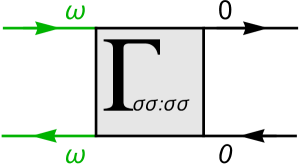
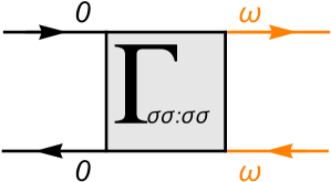
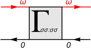
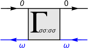
Figure 6: (Color online) Four different ways that the external frequency $\omega$ enters and gets out of the vertex part. These diagrams corresponding to $\Gamma_{\sigma\sigma;\sigma\sigma}(i\omega,0;0,i\omega)$, $\Gamma_{\sigma\sigma;\sigma\sigma}(0,i\omega;i\omega,0)$, $\Gamma_{\sigma\sigma;\sigma\sigma}(i\omega,i\omega;0,0)$, and $\Gamma_{\sigma\sigma;\sigma\sigma}(0,0;i\omega,i\omega)$.

As the total frequencies are conserved, $\omega_{1}+\omega_{3}=\omega_{2}+\omega_{4}$, and three frequencies among the four are independent, we can choose the following $\varepsilon$, $\varepsilon^{\prime}$, and $\nu$ as three independent variables:

$$\omega_{1}=\varepsilon+\nu,\quad\omega_{2}=\varepsilon^{\prime}+\nu,\quad\omega_{3}=\varepsilon^{\prime},\quad\omega_{4}=\varepsilon.$$ (100)

Using these three frequencies, we write the vertex function in an abbreviated form:

$$\Gamma_{\sigma\sigma}(i\varepsilon,i\varepsilon^{\prime};i\nu)\,\equiv\,\Gamma_{\sigma\sigma;\sigma\sigma}(i\varepsilon+i\nu,i\varepsilon^{\prime}+i\nu;i\varepsilon^{\prime},i\varepsilon)\;.$$ (101)

As a function of $\varepsilon$, $\varepsilon^{\prime}$ and $\omega$, the vertex correction for interchanged frequencies, $\omega_{2}\Leftrightarrow\omega_{4}$ and/or $\omega_{1}\Leftrightarrow\omega_{3}$, can be expressed in the form,

$$\widehat{C}_{\mathrm{out}}\Gamma_{\sigma\sigma;\sigma\sigma}(i\varepsilon+i\nu,i\varepsilon^{\prime}+i\nu;i\varepsilon^{\prime},i\varepsilon)$$

$$\qquad\qquad\qquad\qquad=\ \Gamma_{\sigma\sigma}(i\varepsilon^{\prime}+i\nu,i\varepsilon^{\prime};i\varepsilon-i\varepsilon^{\prime}),$$ (102)

$$\widehat{C}_{\mathrm{in}}\,\Gamma_{\sigma\sigma;\sigma\sigma}(i\varepsilon+i\nu,i\varepsilon^{\prime}+i\nu;i\varepsilon^{\prime},i\varepsilon)$$

$$\qquad\qquad\qquad\qquad=\ \Gamma_{\sigma\sigma}(i\varepsilon,i\varepsilon+i\nu;i\varepsilon^{\prime}-i\varepsilon),$$ (103)

$$\widehat{C}_{\mathrm{in}}\widehat{C}_{\mathrm{out}}\,\Gamma_{\sigma\sigma;\sigma\sigma}(i\varepsilon+i\nu,i\varepsilon^{\prime}+i\nu;i\varepsilon^{\prime},i\varepsilon)$$

$$\qquad\qquad\qquad\qquad=\ \Gamma_{\sigma\sigma}(i\varepsilon^{\prime}+i\nu,i\varepsilon+i\nu;-i\nu).$$ (104)

Choosing the frequencies such that $\varepsilon^{\prime}=\nu=0$ and $\varepsilon=\omega$, Eq. (99) can be expressed in the form

$$\!\!\!\!\!\Gamma_{\sigma\sigma;\sigma\sigma}(i\omega,0;0,i\omega)$$

$$=\frac{1}{4}\,\biggl{[}\,\Gamma_{\sigma\sigma}(i\omega,0;0)+\Gamma_{\sigma\sigma}(0,i\omega;0)-\Gamma_{\sigma\sigma}(0,0;i\omega)$$

$$\qquad\ \ -\Gamma_{\sigma\sigma}(i\omega,i\omega;-i\omega)\,\biggr{]}.$$ (105)

The assignment of the frequency $\omega$ for each term is indicated in Fig. 6.

VII.1.1 Total derivative with respect to $\,\widehat{\partial}_{i\omega}^{+}$

The derivative $\widehat{\partial}_{i\omega}^{+}\Gamma_{\sigma\sigma;\sigma\sigma}(i\omega,0;0,i\omega)$ can be carried out using the generalized chain rule which is quite similar to the usual chain rule for differentiation as described in Eq. (86). If the total derivative can be defined for $\widehat{\partial}_{i\omega}^{+}$ such that

$$\!\!\!\!\widehat{\partial}_{i\omega}^{+}\,\Gamma_{\sigma\sigma}(i\omega,i\omega;-i\omega)$$

$$= \ \widehat{\partial}_{i\omega}^{+}\,\Gamma_{\sigma\sigma}(i\omega,0;0)+\widehat{\partial}_{i\omega}^{+}\,\Gamma_{\sigma\sigma}(0,i\omega;0)-\widehat{\partial}_{i\omega}^{+}\,\Gamma_{\sigma\sigma}(0,0;i\omega),$$ (106)

then the result $\zeta_{\sigma}^{R}=0$ will follow from Eq. (105) as

$$\widehat{\partial}_{i\omega}^{+}\,\Gamma_{\sigma\sigma;\sigma\sigma}(i\omega,0;0,i\omega)$$

$$=\,\frac{1}{4}\,\widehat{\partial}_{i\omega}^{+}\biggl{[}\,\Gamma_{\sigma\sigma}(i\omega,0;0)+\Gamma_{\sigma\sigma}(0,i\omega;0)-\Gamma_{\sigma\sigma}(0,0;i\omega)$$

$$\qquad\qquad-\Gamma_{\sigma\sigma}(i\omega,i\omega;-i\omega)\biggr{]}\ =\,0.$$ (107)

This observation can be regarded as another interpretation of the property of the analytic part of $\Gamma_{\sigma\sigma;\sigma\sigma}(i\omega,0;0,i\omega)$ discussed in Sec. IV, i.e., $a_{\sigma\sigma}=0$, which follows from the fact that an anti-symmetric function, which satisfies Eq. (95), cannot be constructed by a homogeneous polynomial of a linear form as shown in Appendix B. We carry out perturbative calculations up to order $U^{4}$ below to show that $\zeta_{\sigma}^{R}=0$.

VII.2 Anti-symmetrized skeleton diagram expansion

We perturbatively calculate the regular part of $\omega$-linear contribution, $\zeta_{\sigma}^{R}$ defined in Eq. (91), operating $\widehat{\partial}_{i\omega}^{+}$ upon $\Gamma_{\sigma\sigma;\sigma\sigma}(i\omega,0;0,i\omega)$, and show diagrammatically how the cancellations that results in $\zeta_{\sigma}^{R}=0$ occur. In order to carry out the calculations in a fully anti-symmetrized way, a standard Bethe-Salpeter type resummation, in which the full vertex function is decomposed into the irreducible part and the iterative ladders of particle-hole-pair propagators, is not useful. We calculate together the contributions of each set that consists of four related diagrams, generated from one of them carrying out the symmetry operations $\widehat{C}_{\mathrm{in}}$, $\widehat{C}_{\mathrm{out}}$, and $\widehat{C}_{\mathrm{in}}\widehat{C}_{\mathrm{out}}$. We explicitly show how the cancellation occurs in the skeleton-diagram expansion, for which the solid lines represent the exact interacting Green’s functions $G_{\sigma}$, up to order $U^{4}$.Note (1)

In the following, we consider the parallel-spin vertex function for $\sigma=\uparrow$ to make the equations simpler as the corresponding result obviously holds for the opposite spin $\sigma=\downarrow$. We choose one arbitrary diagram from the four related diagrams mentioned in the above, and refer to it as representative of the set. The contribution of the representative diagram alone $\Gamma_{\uparrow\uparrow;\uparrow\uparrow}^{(\mathrm{rep})}(i\omega_{1},i\omega_{2};i\omega_{3},i\omega_{4})$ is not an anti-symmetric function but the total contribution of the set $\Gamma_{\uparrow\uparrow;\uparrow\uparrow}^{(\mathrm{set})}$ acquires the anti-symmetry property,

$$\!\!\!\!\!\!\!\!\!\!\Gamma_{\uparrow\uparrow;\uparrow\uparrow}^{(\mathrm{set})}(i\omega,0;0,i\omega)$$

$$= \ \ \Gamma_{\uparrow\uparrow;\uparrow\uparrow}^{(\mathrm{rep})}(i\omega,0;0,i\omega)+\Gamma_{\uparrow\uparrow;\uparrow\uparrow}^{(\mathrm{rep})}(0,i\omega;i\omega,0)$$

$$-\Gamma_{\uparrow\uparrow;\uparrow\uparrow}^{(\mathrm{rep})}(i\omega,i\omega;0,0)-\Gamma_{\uparrow\uparrow;\uparrow\uparrow}^{(\mathrm{rep})}(0,0;i\omega,i\omega)\;.$$ (108)

There is a class of vertex diagrams that graphically have two axes of the reflection symmetry: one in the horizontal direction and the other in the vertical direction. The simplest example is the order $U^{2}$ diagrams shown in Fig. 3. Such sets with an additional symmetry consist of two independent diagrams. Thus, for such sets, we multiply an extra factor $1/2$ to the right-hand side of Eq. (108) for compensating the double counting of the two identical diagrams. We examine the contributions of the first few diagrams in the skeleton-diagram expansion below.

 

 

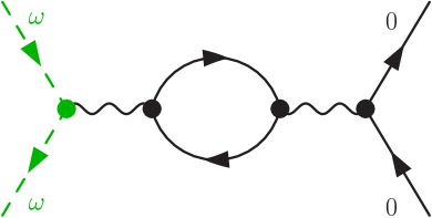
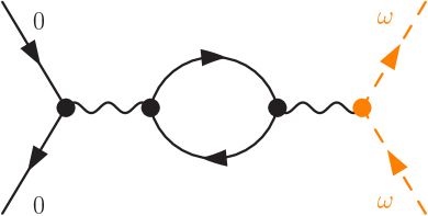
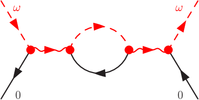
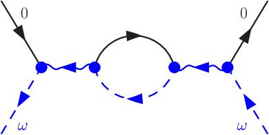
Figure 7: (Color online) A set of four diagrams for $\Gamma_{\uparrow\uparrow;\uparrow\uparrow}^{(2)}$ generated from the first one in the upper left panel by operating $\widehat{C}_{\mathrm{in}}\widehat{C}_{\mathrm{out}}$, $\widehat{C}_{\mathrm{out}}$, and $\widehat{C}_{\mathrm{in}}$. The dashed line represents the propagator that carries the external frequency $\omega$. The wavy lines, which carry $\omega$, are shown with the arrow, indicating the direction $\omega$ flows. In this case, the four diagrams are not independent because the diagram has two different axes of the reflection symmetry.

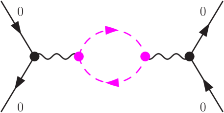
Figure 8: (Color online) Schematic picture expressing the total contribution $\Gamma_{\uparrow\uparrow;\uparrow\uparrow}^{(2)}$ of the diagrams shown in Fig. 7. The dashed propagators carrying the external frequency $\omega$ form a closed loop.

VII.2.1 Order $U^{2}$ contributions

The diagrams for order $U^{2}$ skeleton diagrams for the parallel spins vertex function are described in Fig. 3, and their contribution can be expressed in the form

$$\Gamma_{\uparrow\uparrow;\uparrow\uparrow}^{(2)}(i\omega,0;0,i\omega)\,=\,U^{2}\Bigl{[}\,\chi_{\downarrow\downarrow}^{qp}(i\omega)-\chi_{\downarrow\downarrow}^{qp}(0)\,\Bigr{]}\;,$$ (109)

$$\chi_{\sigma\sigma}^{qp}(i\omega)\,\equiv\,-\int_{-\infty}^{\infty}\!\frac{d\varepsilon}{2\pi}\,G_{\sigma}(i\varepsilon+i\omega)\,G_{\sigma}(i\varepsilon)\,.$$ (110)

We can rewrite this equation in the form of Eq. (108) to make the anti-symmetry property explicit,

$$\!\!\!\!\!\!\!\!\widehat{\partial}_{i\omega}^{+}\,\Gamma_{\uparrow\uparrow;\uparrow\uparrow}^{(2)}(i\omega,0;0,i\omega)$$

$$= \ \frac{U^{2}}{2}\!\int_{-\infty}^{\infty}\frac{d\varepsilon}{2\pi}\ \widehat{\partial}_{i\omega}^{+}\Bigl{[}\,\left\{G_{\downarrow}(i\varepsilon)\right\}^{2}+\,\left\{G_{\downarrow}(i\varepsilon)\right\}^{2}$$

$$\qquad\quad-G_{\downarrow}(i\varepsilon)\,{\color[rgb]{1,0,0}G_{\downarrow}(i\varepsilon+i\omega)}-{\color[rgb]{0,0,1}G_{\downarrow}(i\varepsilon+i\omega)\,}G_{\downarrow}(i\varepsilon)\,\Bigr{]}$$

$$= \ -\frac{U^{2}}{2}\,\ {\color[rgb]{1,0,1}\widehat{\partial}_{i\omega}^{+}\left[\,\int_{-\infty}^{\infty}\frac{d\varepsilon}{2\pi}\,\left\{G_{\downarrow}(i\varepsilon+i\omega)\right\}^{2}\right]}\,=\,0.$$ (111)

The first and second terms of the integrand represent the contributions of the diagrams shown in the upper panel of Fig.  7; the representative and the one generated by $\widehat{C}_{\mathrm{in}}\widehat{C}_{\mathrm{out}}$. Similarly, the third and fourth terms represents the contributions of the diagrams shown in the lower panel; the ones generated by $\widehat{C}_{\mathrm{in}}$ and $\widehat{C}_{\mathrm{out}}$. The second line of Eq. (111) is obtained by using the generalized chain rule given in Eq. (86). It shows that the contribution can be written as a total $\widehat{\partial}_{i\omega}^{+}$ derivative of a definite integral over the circular frequency $\varepsilon$ along the loop which are symbolically illustrated in Fig.  8. The $\omega$ dependence disappears after carrying out the integration over $\varepsilon$ as it can be absorbed into the loop frequency $\varepsilon$. This lowest order example already captures a general feature of the cancellation of the regular part of $\omega$-linear term occurring in the set of four anti-symmetrized diagrams.

VII.2.2 Order $U^{3}$ contributions

 

 

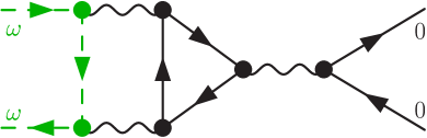
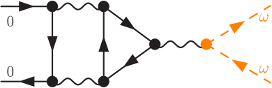
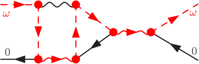
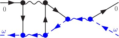
Figure 9: (Color online) A set of four diagrams for $\Gamma_{\uparrow\uparrow;\uparrow\uparrow}^{(3A)}$ generated from the first one in the upper left panel by operating $\widehat{C}_{\mathrm{in}}\widehat{C}_{\mathrm{out}}$, $\widehat{C}_{\mathrm{out}}$, and $\widehat{C}_{\mathrm{in}}$. The dashed line represents the propagator that carries the external frequency $\omega$. The wavy lines, which carry $\omega$, are shown with the arrow, indicating the direction $\omega$ flows.

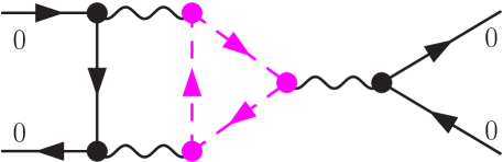
Figure 10: (Color online) Schematic picture expressing the total contribution $\widehat{\partial}_{i\omega}^{+}\Gamma_{\uparrow\uparrow;\uparrow\uparrow}^{(3A)}$ of the diagrams shown in Fig. 9. The dashed propagators carrying the external frequency $\omega$ form a closed loop.

There are two different sets in order $U^{3}$ skeleton diagrams for the parallel-spin vertex function, as shown in Figs. 9 and 11. The contribution of the set of four diagrams in Fig. 9 can be calculated as

$$\widehat{\partial}_{i\omega}^{+}\Gamma_{\uparrow\uparrow;\uparrow\uparrow}^{(3A)}(i\omega,0;0,i\omega)$$

$$=\ U^{3}\int_{-\infty}^{\infty}\int_{-\infty}^{\infty}\frac{d\varepsilon^{\prime}d\varepsilon}{(2\pi)^{2}}\$$

$$\ \times\widehat{\partial}_{i\omega}^{+}\Biggl{[}{\color[rgb]{1,0,0}G_{\uparrow}(i\varepsilon^{\prime}+i\omega)\,G_{\downarrow}(i\varepsilon^{\prime}+i\varepsilon+i\omega)\,G_{\downarrow}(i\varepsilon+i\omega)\,}G_{\downarrow}(i\varepsilon)$$

$$\qquad\quad+G_{\uparrow}(i\varepsilon^{\prime})\,G_{\downarrow}(i\varepsilon^{\prime}+i\varepsilon)\,G_{\downarrow}(i\varepsilon)\,{\color[rgb]{0,0,1}G_{\downarrow}(i\varepsilon+i\omega)\,}$$

$$\qquad\quad-{\color[rgb]{0,0.6,0}G_{\uparrow}(i\varepsilon^{\prime}+i\omega)\,}G_{\downarrow}(i\varepsilon^{\prime}+i\varepsilon)\left\{G_{\downarrow}(i\varepsilon)\right\}^{2}$$

$$\qquad\quad-G_{\uparrow}(i\varepsilon^{\prime})\,G_{\downarrow}(i\varepsilon^{\prime}+i\varepsilon)\left\{G_{\downarrow}(i\varepsilon)\right\}^{2}\Biggr{]}$$

$$=\ U^{3}\int_{-\infty}^{\infty}\int_{-\infty}^{\infty}\frac{d\varepsilon^{\prime}d\varepsilon}{(2\pi)^{2}}\ G_{\uparrow}(i\varepsilon^{\prime})\$$

$$\ \times\widehat{\partial}_{i\omega}^{+}\Biggl{[}\,{\color[rgb]{1,0,0}G_{\downarrow}(i\varepsilon^{\prime}+i\varepsilon+i\omega)\,G_{\downarrow}(i\varepsilon+i\omega)\,}G_{\downarrow}(i\varepsilon)$$

$$\quad+G_{\downarrow}(i\varepsilon^{\prime}+i\varepsilon)\,G_{\downarrow}(i\varepsilon)\,{\color[rgb]{0,0,1}G_{\downarrow}(i\varepsilon+i\omega)\,}$$

$$\quad-G_{\downarrow}(i\varepsilon^{\prime}+i\varepsilon)\left\{G_{\downarrow}(i\varepsilon)\right\}^{2}-G_{\downarrow}(i\varepsilon^{\prime}+i\varepsilon)\left\{G_{\downarrow}(i\varepsilon)\right\}^{2}\,\Biggr{]}$$

$$=\ U^{3}\int_{-\infty}^{\infty}\frac{d\varepsilon^{\prime}}{2\pi}\,G_{\uparrow}(i\varepsilon^{\prime})$$

$$\quad\times{\color[rgb]{1,0,1}\widehat{\partial}_{i\omega}^{+}\Biggl{[}\,\int_{-\infty}^{\infty}\frac{d\varepsilon}{2\pi}\ G_{\downarrow}(i\varepsilon^{\prime}+i\varepsilon+i\omega)\,\left\{G_{\downarrow}(i\varepsilon+i\omega)\right\}^{2}\,\Biggr{]}}$$

$$=\ 0.$$ (112)

To obtain the second line, we have carried out the derivative with respect to $\omega$ assigned for the propagators along the direct line which links the two external propagators on the left side. It can easily be seen that the derivative of the $\uparrow$ spin propagator in the first term and that of the third term cancel each other out. Then, to obtain the next line, the operator $\widehat{\partial}_{i\omega}^{+}$ is applied to the $\downarrow$ spin propagators taking into account the generalized chain rule given in Eq. (86) for the particle-hole product $G_{\downarrow}(i\varepsilon+i\omega)G_{\downarrow}(i\varepsilon)$. In the last line, all the $\downarrow$-spin propagators along the closed loop, which is drawn with dashed lines in Fig. 10, capture the external frequency $\omega$ as their argument, and thus the $\omega$ dependence vanishes after carrying out the integration over the circular frequency $\varepsilon$ along the $\downarrow$-spin loop. Therefore, this example also shows that the contribution of the set of four diagrams on the regular part of the $\omega$-linear dependence can be absorbed into some internal loop frequencies and then it vanishes.

 

 

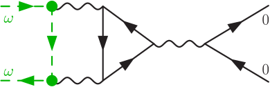
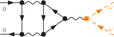
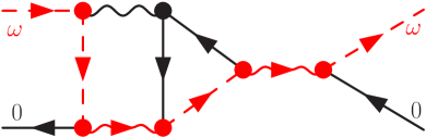
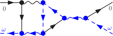
Figure 11: (Color online) A set of four diagrams for $\Gamma_{\uparrow\uparrow;\uparrow\uparrow}^{(3B)}$ generated from the first one in the upper left panel by operating $\widehat{C}_{\mathrm{in}}\widehat{C}_{\mathrm{out}}$, $\widehat{C}_{\mathrm{out}}$, and $\widehat{C}_{\mathrm{in}}$. The dashed line represents the propagator which is assigned to carry the external frequency $\omega$. The wavy line, through which $\omega$ passes, is associated with the arrow showing the direction $\omega$ flows.

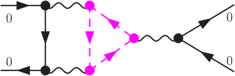
Figure 12: (Color online) Schematic picture expressing the total contribution $\widehat{\partial}_{i\omega}^{+}\Gamma_{\uparrow\uparrow;\uparrow\uparrow}^{(3B)}$ of the diagrams shown in Fig. 11. The dashed propagators carrying the external frequency $\omega$ form a closed loop.

The other order $U^{3}$ set of four skeleton diagrams is in Fig. 11, which has an intermediate particle-particle pair in the vertical direction. The contribution of this set can be calculated in a similar way to the case of the particle-hole pair described in the above,

$$\widehat{\partial}_{i\omega}^{+}\Gamma_{\uparrow\uparrow;\uparrow\uparrow}^{(3B)}(i\omega,0;0,i\omega)$$

$$=\ U^{3}\int_{-\infty}^{\infty}\int_{-\infty}^{\infty}\frac{d\varepsilon^{\prime}d\varepsilon}{(2\pi)^{2}}\$$

$$\ \times\widehat{\partial}_{i\omega}^{+}\Biggl{[}{\color[rgb]{1,0,0}G_{\uparrow}(i\varepsilon^{\prime}+i\omega)\,G_{\downarrow}(i\varepsilon+i\omega)\,}G_{\downarrow}(i\varepsilon-i\varepsilon^{\prime})\,G_{\downarrow}(i\varepsilon)\,$$

$$\qquad\quad+G_{\uparrow}(i\varepsilon^{\prime})\,{\color[rgb]{0,0,1}G_{\downarrow}(i\varepsilon-i\varepsilon^{\prime}+i\omega)\,G_{\downarrow}(i\varepsilon+i\omega)\,}G_{\downarrow}(i\varepsilon)\,$$

$$\qquad\quad-{\color[rgb]{0,0.6,0}G_{\uparrow}(i\varepsilon^{\prime}+i\omega)\,}G_{\downarrow}(i\varepsilon-i\varepsilon^{\prime})\left\{G_{\downarrow}(i\varepsilon)\right\}^{2}$$

$$\qquad\quad-G_{\uparrow}(i\varepsilon^{\prime})\,G_{\downarrow}(i\varepsilon-i\varepsilon^{\prime})\left\{G_{\downarrow}(i\varepsilon)\right\}^{2}\Biggr{]}$$

$$=\ U^{3}\int_{-\infty}^{\infty}\int_{-\infty}^{\infty}\frac{d\varepsilon^{\prime}d\varepsilon}{(2\pi)^{2}}\ G_{\uparrow}(i\varepsilon^{\prime})\$$

$$\ \times\widehat{\partial}_{i\omega}^{+}\Biggl{[}\,G_{\downarrow}(i\varepsilon-i\varepsilon^{\prime})\,G_{\downarrow}(i\varepsilon)\,{\color[rgb]{1,0,0}G_{\downarrow}(i\varepsilon+i\omega)\,}$$

$$\quad+{\color[rgb]{0,0,1}G_{\downarrow}(i\varepsilon-i\varepsilon^{\prime}+i\omega)\,G_{\downarrow}(i\varepsilon+i\omega)\,}G_{\downarrow}(i\varepsilon)\,$$

$$\quad-G_{\downarrow}(i\varepsilon-i\varepsilon^{\prime})\left\{G_{\downarrow}(i\varepsilon)\right\}^{2}-G_{\downarrow}(i\varepsilon-i\varepsilon^{\prime})\left\{G_{\downarrow}(i\varepsilon)\right\}^{2}\,\Biggr{]}$$

$$=\ U^{3}\int_{-\infty}^{\infty}\frac{d\varepsilon^{\prime}}{2\pi}\ G_{\uparrow}(i\varepsilon^{\prime})$$

$$\quad\times{\color[rgb]{1,0,1}\widehat{\partial}_{i\omega}^{+}\Biggl{[}\,\int_{-\infty}^{\infty}\frac{d\varepsilon}{2\pi}\ G_{\downarrow}(i\varepsilon-i\varepsilon^{\prime}+i\omega)\,\left\{G_{\downarrow}(i\varepsilon+i\omega)\right\}^{2}\,\Biggr{]}}$$

$$=\ 0.$$ (113)

To obtain the second line, the derivative with respect to $\omega$ assigned for the propagators along the direct line has been carried out. Then, the derivative of the $\uparrow$ spin propagators in the red first term and that of the green third term cancel out. The next line has been obtained operating $\widehat{\partial}_{i\omega}^{+}$ upon the $\downarrow$ spin propagators along the loop, using the generalized chain rule for the particle-hole product $G_{\downarrow}(i\varepsilon+i\omega)G_{\downarrow}(i\varepsilon)$. The last line again shows that the contribution can be expressed in a total derivative with respect to the loop frequency as illustrated in Fig. 12, and it vanishes.

VII.3 Cancellations in general cases

We summarize how the cancellation which generally occurs for every such set of four anti-symmetrized skeleton diagrams in this subsection. To make the discussion clear, we assign the internal frequencies in such a way as described in the following items $i$)–$iii$), which has already been used in the above:

• We choose the representative $\Gamma_{\uparrow\uparrow;\uparrow\uparrow}^{(\mathrm{rep})}(i\omega,0;0,i\omega)$ to be the contribution of such a diagram in which the external frequency $\omega$ flows along a direct line of $\uparrow$-spin internal propagators towards the exit, i.e., we assign the frequencies along the direct line such that the external $\omega$ does not flow into the wavy interaction lines which link to closed loops. One example is the diagram shown in the upper left panel of Fig. 9, in which the dashed vertical line on the left is in the direct path on the left.

• We choose the second diagram to be the one corresponding to $\Gamma_{\uparrow\uparrow;\uparrow\uparrow}^{(\mathrm{rep})}(0,i\omega;i\omega,0)$ which can be generated by the symmetry operation $\widehat{C}_{\mathrm{in}}\widehat{C}_{\mathrm{out}}\Gamma_{\uparrow\uparrow;\uparrow\uparrow}^{(\mathrm{rep})}(i\omega,0;0,i\omega)$. In the diagram of this category, the external $\omega$ flows through the other direct $\uparrow$ spin path. An example of this type is shown in the upper right panel of Fig. 9, in which the dashed lines on the right correspond to the direct path of this category.

• The remaining two terms $\Gamma_{\uparrow\uparrow;\uparrow\uparrow}^{(\mathrm{rep})}(i\omega,i\omega;0,0)$ and $\Gamma_{\uparrow\uparrow;\uparrow\uparrow}^{(\mathrm{rep})}(0,0;i\omega,i\omega)$ are generated by operating $\widehat{C}_{\mathrm{out}}$ and $\widehat{C}_{\mathrm{in}}$ upon the representative. In the diagrams of this two categories, the external frequency $\omega$ enters into the vertex part on the one side and gets out from the other side, passing through interaction lines and closed loops in the central region. An example that is derived from $\widehat{C}_{\mathrm{out}}$ and that from $\widehat{C}_{\mathrm{in}}$ are shown in the lower-left and lower-right panels of Fig. 9, for which the frequencies are chosen such that the external $\omega$ flows along the dashed lines. For simplicity, we assign the internal frequencies for $\Gamma_{\uparrow\uparrow;\uparrow\uparrow}^{(\mathrm{rep})}(i\omega,i\omega;0,0)$ and that for $\Gamma_{\uparrow\uparrow;\uparrow\uparrow}^{(\mathrm{rep})}(0,0;i\omega,i\omega)$ in a synchronized way such that the external $\omega$ passes through the same interaction line. Such interaction lines are denoted by dashed wavy lines with an arrow that indicates the direction the $\omega$ flows.

 

 

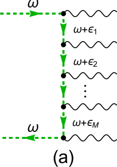
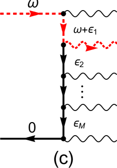
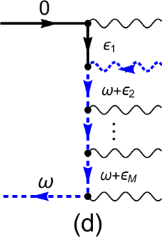
Figure 13: (Color online) The direct line on the left side of (a): $\Gamma_{\uparrow\uparrow;\uparrow\uparrow}^{(\mathrm{rep})}(i\omega,0;0,i\omega)$, (b): $\Gamma_{\uparrow\uparrow;\uparrow\uparrow}^{(\mathrm{rep})}(0,i\omega;i\omega,0)$, (c): $\Gamma_{\uparrow\uparrow;\uparrow\uparrow}^{(\mathrm{rep})}(i\omega,i\omega;0,0)$, and (d): $\Gamma_{\uparrow\uparrow;\uparrow\uparrow}^{(\mathrm{rep})}(0,0;i\omega,i\omega)$. The dashed lines denote the propagators and interaction lines that carry the external frequency $\omega$.

 

 

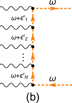
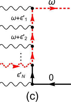
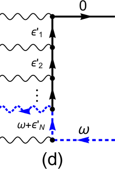
Figure 14: (Color online) The direct line on the right side of (a): $\Gamma_{\uparrow\uparrow;\uparrow\uparrow}^{(\mathrm{rep})}(i\omega,0;0,i\omega)$, (b): $\Gamma_{\uparrow\uparrow;\uparrow\uparrow}^{(\mathrm{rep})}(0,i\omega;i\omega,0)$, (c): $\Gamma_{\uparrow\uparrow;\uparrow\uparrow}^{(\mathrm{rep})}(i\omega,i\omega;0,0)$, and (d): $\Gamma_{\uparrow\uparrow;\uparrow\uparrow}^{(\mathrm{rep})}(0,0;i\omega,i\omega)$. The dashed lines denote the propagators and interaction lines that carry the external frequency $\omega$.

We calculate together the contributions of the four diagrams which constitutes the set, $\widehat{\partial}_{i\omega}^{+}\Gamma_{\uparrow\uparrow;\uparrow\uparrow}^{(\mathrm{set})}(i\omega,0;0,i\omega)$ in order to keep the anti-symmetry of the vertex function. It can be shown that the contribution of the propagators which belong to one of the two direct $\uparrow$ lines vanishes, as seen in the middle part of Eqs. (112) and (113) for the order $U^{3}$ contributions. This is owing to the anti-symmetry, and can be confirmed by operating $\widehat{\partial}_{i\omega}^{+}$ upon the direct lines as shown in Figs.  13 and 14.

The remaining contributions can be generated, operating $\widehat{\partial}_{i\omega}^{+}$ upon the closed loops, which partially carry $\omega$. In our construction of the diagrams, such contributions arise from $\Gamma_{\uparrow\uparrow;\uparrow\uparrow}^{(\mathrm{rep})}(i\omega,i\omega;0,0)$ and $\Gamma_{\uparrow\uparrow;\uparrow\uparrow}^{(\mathrm{rep})}(0,0;i\omega,i\omega)$. The corresponding order $U^{3}$ diagrams are described in the lower panel of Figs. 9 and 11. The contributions of the two diagrams cancel out as the external $\omega$ is absorbed into the circular frequency along the closed loop as shown in Figs.  10 and 12. Figure 15 describes the same cancellation occurring in a single but a more complicated loop. As we construct Figs.  15 (a) and (b) following rule $iii$) such that the external frequency $\omega$ passes through the same interaction lines, their contributions of the loop part can be written in the form

$$I^{(a)}_{\sigma^{\prime\prime}}= \ \ \widehat{\partial}_{i\omega}^{+}\Biggl{[}\int_{-\infty}^{\infty}\frac{d\varepsilon}{2\pi}\,{\color[rgb]{1,0,0}G_{\sigma^{\prime\prime}}(i\varepsilon+i\omega)}\,G_{\sigma^{\prime\prime}}(i\varepsilon)$$

$$\qquad\times\prod_{j}^{N}G_{\sigma^{\prime\prime}}(i\varepsilon+i\varepsilon_{a_{j}})\,{\color[rgb]{1,0,0}\prod_{k}^{M}G_{\sigma^{\prime\prime}}(i\varepsilon+i\omega+i\varepsilon_{b_{k}})}\Biggr{]},$$ (114)

$$I^{(b)}_{\sigma^{\prime\prime}}= \ \ \widehat{\partial}_{i\omega}^{+}\Biggl{[}\int_{-\infty}^{\infty}\frac{d\varepsilon}{2\pi}\,G_{\sigma^{\prime\prime}}(i\varepsilon)\,{\color[rgb]{0,0,1}G_{\sigma^{\prime\prime}}(i\varepsilon+i\omega)}$$

$$\qquad\times{\color[rgb]{0,0,1}\prod_{j}^{N}G_{\sigma^{\prime\prime}}(i\varepsilon+\omega+i\varepsilon_{a_{j}})}\,\prod_{k}^{M}G_{\sigma^{\prime\prime}}(i\varepsilon+i\varepsilon_{b_{k}})\Biggr{]}.$$ (115)

The sum of these two contributions can be described by a single diagram Fig.  15 (c),

$$I^{(a)}_{\sigma^{\prime\prime}}+I^{(b)}_{\sigma^{\prime\prime}}\ =\ \widehat{\partial}_{i\omega}^{+}\,\Biggl{[}\int_{-\infty}^{\infty}\frac{d\varepsilon}{2\pi}\,{\color[rgb]{1,0,1}\left\{G_{\sigma^{\prime\prime}}(i\varepsilon+i\omega)\right\}^{2}}$$

$$\times{\color[rgb]{1,0,1}\prod_{j}^{N}G_{\sigma^{\prime\prime}}(i\varepsilon+i\omega+i\varepsilon_{a_{j}})\,\prod_{k}^{M}G_{\sigma^{\prime\prime}}(i\varepsilon+i\omega+i\varepsilon_{b_{k}})}\Biggr{]}=0.$$ (116)

Here, the integration over $\varepsilon$ gives a constant that is independent of $\omega$.

For more complicated diagrams, the external frequency $\omega$ passes through a number of different closed loops, but the contribution from each of such closed loops vanishes in a similar way to Eq. (116). We have also calculated all the skeleton-diagrams for $\Gamma_{\sigma\sigma;\sigma\sigma}(i\omega,0;0,i\omega)$ up to order $U^{4}$.Note (1) It explicitly shows that the cancellation of the analytic $\omega$-linear part occurs for each and every set of four anti-symmetrized diagrams.

 

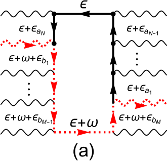
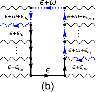
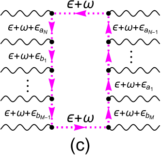
Figure 15: (Color online) Example of a closed loop that includes one singular particle-hole product $G_{\sigma^{\prime\prime}}(i\varepsilon)\,G_{\sigma^{\prime\prime}}(i\varepsilon+i\omega)$ for (a): $\Gamma_{\uparrow\uparrow;\uparrow\uparrow}^{(\mathrm{rep})}(i\omega,i\omega;0,0)$, and (b): $\Gamma_{\uparrow\uparrow;\uparrow\uparrow}^{(\mathrm{rep})}(0,0;i\omega,i\omega)$. Total contribution of (a) and (b) coincides with the contribution of (c), or symbolically $\widehat{\partial}_{i\omega}^{+}\Bigl{[}(a)\,+\,(b)\Bigr{]}=\widehat{\partial}_{i\omega}^{+}\Bigl{[}(c)\Bigr{]}$. In (c), the external frequency $\omega$ flows along the loop, and thus it can be integrated out with the circular frequency $\varepsilon$, i.e., $\widehat{\partial}_{i\omega}^{+}\int_{-\infty}^{\infty}d\varepsilon\,\Bigl{[}(c)\Bigr{]}=0$.

VIII Summary

In summary, we have provided a precise derivation of the higher-order Fermi-liquid relations of the Anderson impurity model. One of the most important results is the double-frequency expansion of the vertex function $\Gamma_{\sigma\sigma^{\prime};\sigma^{\prime}\sigma}(i\omega,i\omega^{\prime};i\omega^{\prime},i\omega)$, given in Eqs.  (51) and (52). These two equations have been deduced from the analytic and anti-symmetric properties of the vertex function: the linear terms with respect to these frequencies must be described by a linear combination of the analytic $\omega$ and $\omega^{\prime}$ contributions and the non-analytic $|\omega-\omega^{\prime}|$ and $|\omega+\omega^{\prime}|$ contributions. In addition, the anti-symmetry imposes the restriction: the vertex function for parallel spins $\sigma^{\prime}=\sigma$ does not have the analytic $\omega$ and $\omega^{\prime}$ contributions. The coefficients for these terms have been determined using the Ward identities. The explicit form of $\Gamma_{\sigma\sigma^{\prime};\sigma^{\prime}\sigma}(i\omega,i\omega^{\prime};i\omega^{\prime},i\omega)$ captures the essential features of the Fermi liquid away from half-filling, and is analogous to Landau’s quasi-particle interaction $f(\bm{p}\,\sigma,\bm{p}^{\prime}\sigma^{\prime})$ and Nozières’ function $\phi_{\sigma\sigma^{\prime}}(\varepsilon,\varepsilon^{\prime})$. Abrikosov et al. (1965); Nozières (1974) One important difference is that the vertex function also has a non-analytic part, which directly determines the damping of the quasi-particles.

In the second half of the present paper, we have also provided a complementary perturbative proof for the low-frequency behavior of the vertex function. For this purpose, we have introduced an operator that can extract the next-leading contribution from a singular Green’s-function product expansion, Eq. (77), for the intermediate particle-hole pair. Specifically, we have calculated all the skeleton-diagrams for $\Gamma_{\sigma\sigma;\sigma\sigma}(i\omega,0;0,i\omega)$ up to order $U^{4}$,Note (1) and have directly confirmed that a cancellation of the analytic $\omega$-linear part occurs in a set of four related Feynman diagrams which anti-symmetrize the vertex corrections.

The higher-order Fermi-liquid corrections away from half-filling are determined not only by the linear susceptibilities $\chi_{\sigma\sigma^{\prime}}$ but also the non-linear susceptibilities $\chi_{\sigma_{1},\sigma_{2},\ldots,\sigma_{n}}^{[n]}$ for $n=3$ and $n=4$. We have also revisited the $T^{2}$-correction of the self-energy $\Sigma_{\sigma}(i\omega)$ for calculating the real part which becomes finite away from half-filling, and have shown that the coefficient is given by $(\pi^{2}/6\rho_{d\sigma})\,\partial\chi_{\uparrow\downarrow}/\partial\epsilon_{d,-\sigma}$. Our result for the $\omega^{2}$ real part, $\mathrm{Re}\left.\partial^{2}\Sigma_{\sigma}(i\omega)/\partial(i\omega)^{2}\right|_{\omega=0}=\partial^{2}\Sigma_{\sigma}(0)/\partial\epsilon_{d\sigma}^{2}$, reproduces exactly the FMvDM’s formula.Filippone et al. (2017) We will give a more detailed comparison in a separate paper, i.e., paper III.Oguri and Hewson (2018)

In paper III, we will also present an extension of the microscopic description to the non-equilibrium steady state driven by the bias voltage $eV$ using the Keldysh formalism. Furthermore, we calculate the Fermi-liquid parameters using the NRG, and will demonstrate applications to various systems such as the non-linear magneto-conductance through a quantum dot, thermo-electric transport of dilute magnetic alloys, and the Anderson impurity with a number orbitals.

Appendix A Static non-linear response functions

We show that $\chi_{\sigma_{1}\sigma_{2}\sigma_{3}}^{[3]}$ can be expressed in terms of three-body correlation functions of the electron configuration of the impurity site, defined with respect to thermal equilibrium. We consider the Hamiltonian, $\mathcal{H}_{\mathrm{tot}}=\mathcal{H}+\mathcal{H}_{\mathrm{ex}}$, which includes a static external part $\mathcal{H}_{\mathrm{ex}}$. Following the standard perturbation theory, the imaginary-time evolution operator ${\cal U}\equiv e^{\beta\mathcal{H}}e^{-\beta\mathcal{H}_{\mathrm{tot}}}$ can be expanded in a power series of $\mathcal{H}_{\mathrm{ex}}$:

$$\!\!\!{\cal U}\,=\,1-\int_{0}^{\beta}\!d\tau_{1}\,\mathcal{H}_{\mathrm{ex}}(\tau_{1})$$

$$\quad+\,\frac{1}{2!}\int_{0}^{\beta}\!d\tau_{1}\!\int_{0}^{\beta}\!d\tau_{2}\,T_{\tau}\bigl{[}\mathcal{H}_{\mathrm{ex}}(\tau_{1})\,\mathcal{H}_{\mathrm{ex}}(\tau_{2})\bigr{]}+\cdots,$$ (117)

where $\beta=1/T$. The average of an operator $\mathcal{O}$ is defined by

$$\langle\mathcal{O}\rangle_{\mathrm{tot}}\equiv\frac{\mathrm{Tr}\left[e^{-\beta\,\mathcal{H}_{\mathrm{tot}}}\,\mathcal{O}\right]}{\mathrm{Tr}\,e^{-\beta\,\mathcal{H}_{\mathrm{tot}}}}=\frac{\left\langle\,{\cal U}(\beta)\,\mathcal{O}\,\right\rangle}{\left\langle\,{\cal U}(\beta)\,\right\rangle},$$ (118)

where $\left\langle\,\cdots\,\right\rangle\,\equiv\,\mathrm{Tr}\left[\,e^{-\beta\,\mathcal{H}}\,\cdots\,\right]\,/\,\Xi$, and $\Xi\,\equiv\,\mathrm{Tr}\,e^{-\beta\,\mathcal{H}}$. For the operator $\delta\mathcal{O}\equiv\mathcal{O}-\langle\mathcal{O}\rangle$ that satisfies $\langle\delta\mathcal{O}\rangle=0$, the expansion up to second order is given by

$$\langle\delta\mathcal{O}\rangle_{\mathrm{tot}}=\,-\int_{0}^{\beta}\!\!\!d\tau\,\langle\mathcal{H}_{\mathrm{ex}}(\tau)\,\delta\mathcal{O}\rangle$$

$$\qquad\quad+\frac{1}{2}\int_{0}^{\beta}\!\!\!d\tau\!\!\int_{0}^{\beta}\!\!\!d\tau^{\prime}\,\langle T_{\tau}\mathcal{H}_{\mathrm{ex}}(\tau)\,\mathcal{H}_{\mathrm{ex}}(\tau^{\prime})\,\delta\mathcal{O}\rangle$$

$$\qquad\quad-\int_{0}^{\beta}\!\!\!d\tau\!\!\int_{0}^{\beta}\!\!\!d\tau^{\prime}\,\langle\mathcal{H}_{\mathrm{ex}}(\tau)\,\delta\mathcal{O}\rangle\,\langle\mathcal{H}_{\mathrm{ex}}(\tau^{\prime})\rangle+\cdots.$$ (119)

We can apply this formula to a response of the occupation number $\mathcal{O}=n_{d\sigma}$ against a small variation of the impurity level $\delta\epsilon_{d\sigma}$, for which the perturbation Hamiltonian is given by $\mathcal{H}_{\mathrm{ex}}=\sum_{\sigma}\delta\epsilon_{d\sigma}\,\delta n_{d\sigma}$ with $\delta n_{d\sigma}\equiv n_{d\sigma}-\langle n_{d\sigma}\rangle$. For this case, $\langle\mathcal{H}_{\mathrm{ex}}(\tau^{\prime})\rangle=0$ by definition, and thus

$$\langle\delta n_{d\sigma}\rangle_{\mathrm{tot}}\,=\,-\sum_{\sigma_{1}}\int_{0}^{\beta}\!\!\!d\tau\,\langle\delta n_{d\sigma_{1}}(\tau)\,\delta n_{d\sigma}\rangle\,\delta\epsilon_{d\sigma_{1}}$$

$$+\frac{1}{2}\!\sum_{\sigma_{1}\sigma_{2}}\!\int_{0}^{\beta}\!\!\!\!d\tau_{1}\!\!\!\int_{0}^{\beta}\!\!\!\!d\tau_{2}\,\langle T_{\tau}\delta n_{d\sigma_{1}}(\tau_{1})\delta n_{d\sigma_{2}}(\tau_{2})\delta n_{d\sigma}\rangle\delta\epsilon_{d\sigma_{1}}\delta\epsilon_{d\sigma_{2}}$$

$$+\cdots.$$ (120)

In this case, the impurity level is given by $\epsilon_{d\sigma}+\delta\epsilon_{d\sigma}$. The coefficients can also be written in terms of the derivative of $\langle n_{d\sigma}\rangle$ with respect to $\epsilon_{d\sigma^{\prime}}$,

$$\chi_{\sigma\sigma^{\prime}}= \ -\frac{\partial\langle n_{d\sigma}\rangle}{\partial\epsilon_{d\sigma^{\prime}}}=\int^{\beta}\!d\tau\,\left\langle\delta n_{d\sigma^{\prime}}(\tau)\,\delta n_{d\sigma}\right\rangle,$$ (121)

$$\chi_{\sigma\sigma_{1}\sigma_{2}}^{[3]}= -\frac{\partial^{2}\langle n_{d\sigma}\rangle}{\partial\epsilon_{d\sigma_{1}}\partial\epsilon_{d\sigma_{2}}}$$

$$= \ -\int_{0}^{\beta}\!\!\!d\tau_{1}\!\!\int_{0}^{\beta}\!\!\!d\tau_{2}\,\langle T_{\tau}\delta n_{d\sigma_{1}}(\tau_{1})\,\delta n_{d\sigma_{2}}(\tau_{2})\,\delta n_{d\sigma}\rangle.$$ (122)

Appendix B Anti-symmetrization of a homogeneous polynomial

We describe here a quite simple but an important property of a homogeneous polynomial of a linear form, i.e., it can not be anti-symmetrized in the following sense. We consider the homogeneous function of degree one,

$$\mathcal{F}(x_{1},x_{2};x_{3},x_{4})\,=\,a_{1}\,x_{1}+a_{2}\,x_{2}+a_{3}\,x_{3}+a_{4}x_{4}\;.$$ (123)

Here, $a_{1}$, $a_{2}$, $a_{3}$, and $a_{4}$ are constants. We set a requirement $x_{1}+x_{3}=x_{2}+x_{4}$ which corresponds to a frequency conservation, and thus three variables among four are independent. Introducing another variable $y$ such that $x_{1}=x_{4}+y$ and $x_{2}=x_{3}+y$, we choose $x_{3}$, $x_{4}$, and $y$ as three independent variables.

In order to anti-symmetrize this polynomial, we impose the additional conditions,

$$\mathcal{F}(x_{1},x_{2};x_{3},x_{4})\,=\,\mathcal{F}(x_{3},x_{4};x_{1},x_{2})$$

$$\qquad=\,-\mathcal{F}(x_{3},x_{2};x_{1},x_{4})\,=\,-\mathcal{F}(x_{1},x_{4};x_{3},x_{2})\;.$$ (124)

These conditions can explicitly be written as,

$$\ (a_{1}+a_{4})\,x_{4}+(a_{2}+a_{3})\,x_{3}+(a_{1}+a_{2})\,y$$

$$= \ \ \ (a_{2}+a_{3})\,x_{4}+(a_{1}+a_{4})\,x_{3}+(a_{3}+a_{4})\,y$$

$$= \ -(a_{3}+a_{4})\,x_{4}-(a_{1}+a_{2})\,x_{3}-(a_{2}+a_{3})\,y$$

$$= \ -(a_{1}+a_{2})\,x_{4}-(a_{3}+a_{4})\,x_{3}-(a_{1}+a_{4})\,y\;.$$ (125)

For these conditions to be identically satisfied for arbitrary $x_{3}$, $x_{4}$, and $y$,

$$a_{1}+a_{4}\,=\,a_{2}+a_{3}\,=\,-(a_{1}+a_{2})\,=\,-(a_{3}+a_{4})\;.$$ (126)

The solution is $a_{1}=-a_{2}=a_{3}=-a_{4}$, and the anti-symmetrized function is given by

$$\mathcal{F}(x_{1},x_{2};x_{3},x_{4})\,=\,a_{1}\,(x_{1}-x_{2}+x_{3}-x_{4})\,\equiv\,0\;,$$ (127)

because $x_{1}+x_{3}=x_{2}+x_{4}$.

We note that this simple property of the homogeneous polynomial justifies our observation that the vertex function for the parallel spins, $\Gamma_{\sigma\sigma;\sigma\sigma}(i\omega_{1},i\omega_{2};i\omega_{3},i\omega_{4})$, does not have the analytic component in the $\omega$-linear terms.

Appendix C The $\omega^{2}$ contribution of $\Gamma_{\sigma,-\sigma;-\sigma,\sigma}(i\omega,0;0,i\omega)$

The coefficient for the $(i\omega)^{2}\,\mathrm{sgn}\,\omega$ term of $\Gamma_{\sigma,-\sigma;-\sigma,\sigma}(i\omega,0;0,i\omega)$ shown in Eqs. (47) is calculated rewriting the derivative in the following way,

$$\frac{\partial}{\partial\epsilon_{d,-\sigma}}\left(\frac{\chi_{\uparrow\downarrow}^{2}}{\rho_{d\sigma}}\right) =\,\frac{2\chi_{\uparrow\downarrow}}{\rho_{d\sigma}}\,\frac{\partial\chi_{\uparrow\downarrow}}{\partial\epsilon_{d,-\sigma}}+2\pi\cot\delta_{\sigma}\,\frac{\chi_{\uparrow\downarrow}^{3}}{\rho_{d\sigma}}$$

$$\xrightarrow{\,h\to 0\,} \ \ \frac{\chi_{\uparrow\downarrow}}{\rho_{d}}\,\left(\frac{\partial\chi_{\uparrow\downarrow}}{\partial\epsilon_{d}}+2\pi\cot\delta\ \chi_{\uparrow\downarrow}^{2}\right)$$ (128)

$$\xrightarrow{\xi_{d}\to 0} \ \ 0\,.$$ (129)

The $(i\omega)^{2}$ part of $\Gamma_{\sigma,-\sigma;-\sigma,\sigma}(i\omega,0;0,i\omega)$ involves the fourth derivative of $\Omega$,

$$\frac{\partial}{\partial\epsilon_{d,-\sigma}}\left(\frac{\partial\widetilde{\chi}_{\sigma\sigma}}{\partial\epsilon_{d\sigma}}\right)\ =\ \frac{\partial^{2}\widetilde{\chi}_{\sigma,-\sigma}}{\partial\epsilon_{d\sigma}^{2}}\ =\ \frac{\partial^{2}}{\partial\epsilon_{d\sigma}^{2}}\left(\frac{\chi_{\uparrow\downarrow}}{\rho_{d\sigma}}\right)$$

$$=\ \frac{1}{\rho_{d\sigma}}\,\frac{\partial^{2}\chi_{\uparrow\downarrow}}{\partial\epsilon_{d\sigma}^{2}}+2\,\frac{\partial\chi_{\uparrow\downarrow}}{\partial\epsilon_{d\sigma}}\,\frac{\partial}{\partial\epsilon_{d\sigma}}\left(\frac{1}{\rho_{d\sigma}}\right)+\chi_{\uparrow\downarrow}\,\frac{\partial^{2}}{\partial\epsilon_{d\sigma}^{2}}\left(\frac{1}{\rho_{d\sigma}}\right)$$

$$=\ \frac{1}{\rho_{d\sigma}}\,\frac{\partial^{2}\chi_{\uparrow\downarrow}}{\partial\epsilon_{d\sigma}^{2}}+\frac{2\pi^{2}\left(2\cos^{2}\delta_{\sigma}+1\right)}{\rho_{d\sigma}\sin^{2}\delta_{\sigma}}\,\chi_{\uparrow\downarrow}\chi_{\sigma\sigma}^{2}$$

$$\quad+\frac{2\pi\cot\delta_{\sigma}}{\rho_{d\sigma}}\left(2\,\chi_{\sigma\sigma}\,\frac{\partial\chi_{\uparrow\downarrow}}{\partial\epsilon_{d\sigma}}+\chi_{\uparrow\downarrow}\frac{\partial\chi_{\sigma\sigma}}{\partial\epsilon_{d\sigma}}\right).$$ (130)

We have used Eq. (21) for the double derivative of the inverse density of states and

$$\frac{\partial^{2}}{\partial\epsilon_{d\sigma}^{2}}\left(\frac{1}{\rho_{d\sigma}}\right)=\ \frac{2\pi\cot\delta_{\sigma}}{\rho_{d\sigma}}\frac{\partial\chi_{\sigma\sigma}}{\partial\epsilon_{d\sigma}}+\frac{2\pi\chi_{\sigma\sigma}^{2}}{\Delta\rho_{d\sigma}^{2}}\left(2\cos^{2}\delta_{\sigma}+1\right).$$ (131)

Equation (130) simplifies in zero magnetic field, and in the particle-hole symmetric case:

$$\frac{\partial}{\partial\epsilon_{d,-\sigma}}\left(\frac{\partial\widetilde{\chi}_{\sigma\sigma}}{\partial\epsilon_{d\sigma}}\right)$$

$$\xrightarrow{h\to 0}\ \frac{1}{4\rho_{d}}\left(\frac{\partial^{2}}{\partial\epsilon_{d}^{2}}+\frac{\partial^{2}}{\partial h^{2}}\right)\chi_{\uparrow\downarrow}+\frac{2\pi^{2}\left(2\cos^{2}\delta+1\right)}{\rho_{d\sigma}\sin^{2}\delta}\,\chi_{\uparrow\downarrow}\chi_{\uparrow\uparrow}^{2}$$

$$\qquad\quad+\frac{2\pi\cot\delta}{\rho_{d}}\left[\left(\chi_{\uparrow\uparrow}-\frac{1}{2}\chi_{\uparrow\downarrow}\right)\frac{\partial\chi_{\uparrow\downarrow}}{\partial\epsilon_{d}}+\chi_{\uparrow\downarrow}\frac{\partial\chi_{\uparrow\uparrow}}{\partial\epsilon_{d}}\right]$$ (132)

$$\xrightarrow{h\to 0\atop\xi_{d}\to 0}\ \pi\Delta\,\left[\frac{1}{4}\left(\frac{\partial^{2}\chi_{\uparrow\downarrow}}{\partial\epsilon_{d}^{2}}+\frac{\partial^{2}\chi_{\uparrow\downarrow}}{\partial h^{2}}\right)+2\pi^{2}\chi_{\uparrow\downarrow}\,\chi_{\uparrow\uparrow}^{2}\right].$$ (133)

In this supplemental materials, we consider the order $U^{4}$ skeleton diagrams of the vertex function for parallel spins to show how the $\omega$-linear regular contributions cancel each other out. Specifically, we calculate the contributions by operating $\widehat{\partial}_{i\omega}^{+}$, defined in Sec. VI of the text, upon $\Gamma_{\uparrow\uparrow;\uparrow\uparrow}(i\omega,0;0,i\omega)$.

 

 

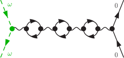
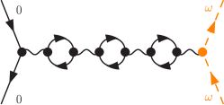
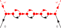
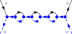
Figure 16: (Color online) A set of four diagrams for $\Gamma_{\uparrow\uparrow;\uparrow\uparrow}^{(4A)}$, contribution of which is given in Eq. (134). The dashed line represents the propagator which is assigned to carry the external frequency $\omega$.

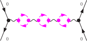
Figure 17: (Color online) Schematic picture for the total contribution $\widehat{\partial}_{i\omega}^{+}\Gamma_{\uparrow\uparrow;\uparrow\uparrow}^{(4A)}$ of the set shown in Fig. 16.

Total contribution of the diagrams shown in Fig. 16 can be rewritten in a total derivative form (see also Fig. 17) :

$$\!\!\!\!\!\!\!\!\!\!\!\!\!\widehat{\partial}_{i\omega}^{+}\Gamma_{\uparrow\uparrow;\uparrow\uparrow}^{(4A)}(i\omega,0;0,i\omega)\,=\,U^{4}\,\widehat{\partial}_{i\omega}^{+}\left[\,\left\{\chi_{\downarrow\downarrow}^{qp}(i\omega)\right\}^{2}\chi_{\uparrow\uparrow}^{qp}(i\omega)-\left\{\chi_{\downarrow\downarrow}^{qp}(0)\right\}^{2}\chi_{\uparrow\uparrow}^{qp}(0)\,\right]$$

$$\,=\,-U^{4}\!\int_{-\infty}^{\infty}\!\int_{-\infty}^{\infty}\!\int_{-\infty}^{\infty}\!\frac{d\varepsilon_{1}\,d\varepsilon_{2}\,d\varepsilon_{3}}{(2\pi)^{3}}\ \widehat{\partial}_{i\omega}^{+}\Bigl{[}G_{\downarrow}(i\varepsilon_{1})\,G_{\downarrow}(i\varepsilon_{1}+i\omega)\,G_{\uparrow}(i\varepsilon_{2})\,G_{\uparrow}(i\varepsilon_{2}+i\omega)\,G_{\downarrow}(i\varepsilon_{3})\,G_{\downarrow}(i\varepsilon_{3}+\omega)\Bigr{]}$$

$$\,=\,-U^{4}\,\frac{1}{2}\,{\color[rgb]{1,0,1}\widehat{\partial}_{i\omega}^{+}\left[\int_{-\infty}^{\infty}\!\int_{-\infty}^{\infty}\!\int_{-\infty}^{\infty}\!\frac{d\varepsilon_{1}\,d\varepsilon_{2}\,d\varepsilon_{3}}{(2\pi)^{3}}\ \left\{G_{\downarrow}(i\varepsilon_{1}+\omega)\right\}^{2}\left\{G_{\uparrow}(i\varepsilon_{2}+i\omega)\right\}^{2}\left\{G_{\downarrow}(i\varepsilon_{3}+i\omega)\right\}^{2}\right]}\ =\ 0.$$ (134)

For this set, the external frequency $\omega$ transverses through the three intermediate closed loops.

 

 

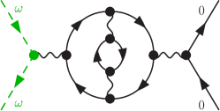
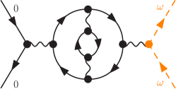
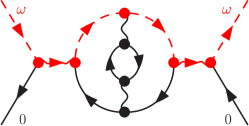
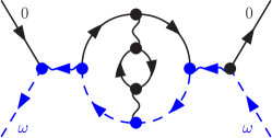
Figure 18: (Color online) A set of four diagrams for $\Gamma_{\uparrow\uparrow;\uparrow\uparrow}^{(4B)}$, contribution of which is given in Eq. (135).

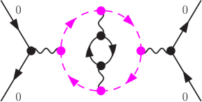
Figure 19: (Color online) Schematic picture for the total contribution $\widehat{\partial}_{i\omega}^{+}\Gamma_{\uparrow\uparrow;\uparrow\uparrow}^{(4B)}$ of the diagrams shown in Fig. 18.

Total contribution of the diagrams shown in Fig. 18 can be rewritten in a total derivative form (see also Fig. 19):

$$\!\!\!\!\!\!\!\!\!\!\!\!\!\widehat{\partial}_{i\omega}^{+}\Gamma_{\uparrow\uparrow;\uparrow\uparrow}^{(4B)}(i\omega,0;0,i\omega)\,=\,-U^{4}\!\int_{-\infty}^{\infty}\!\!\int_{-\infty}^{\infty}\!\!d\varepsilon^{\prime}d\varepsilon\ \widehat{\partial}_{i\omega}^{+}\Bigl{[}\,G_{\downarrow}(i\varepsilon)\,G_{\downarrow}(i\varepsilon+i\omega)\,G_{\downarrow}(i\varepsilon^{\prime})\,G_{\downarrow}(i\varepsilon^{\prime}+i\omega)\,\,-\,\left\{G_{\downarrow}(i\varepsilon)\right\}^{2}\left\{G_{\downarrow}(i\varepsilon^{\prime})\right\}^{2}\,\Bigr{]}\chi_{\uparrow\uparrow}^{qp}(i\varepsilon-i\varepsilon^{\prime})$$

$$=\ -U^{4}\!\int_{-\infty}^{\infty}\!\!\int_{-\infty}^{\infty}\!\!d\varepsilon^{\prime}d\varepsilon\,\Biggl{\{}\widehat{\partial}_{i\omega}^{+}\Bigl{[}\,G_{\downarrow}(i\varepsilon)\,G_{\downarrow}(i\varepsilon+i\omega)\,\Bigr{]}\left\{G_{\downarrow}(i\varepsilon^{\prime})\right\}^{2}+\left\{G_{\downarrow}(i\varepsilon)\right\}^{2}\widehat{\partial}_{i\omega}^{+}\Bigl{[}\,G_{\downarrow}(i\varepsilon^{\prime})\,G_{\downarrow}(i\varepsilon^{\prime}+i\omega)\,\Bigr{]}\,\Biggr{\}}\,\chi_{\uparrow\uparrow}^{qp}(i\varepsilon-i\varepsilon^{\prime})$$

$$=\,-U^{4}\,\frac{1}{2}\,{\color[rgb]{1,0,1}\widehat{\partial}_{i\omega}^{+}\left[\,\int_{-\infty}^{\infty}\!\!\int_{-\infty}^{\infty}\!\!d\varepsilon^{\prime}d\varepsilon\,\left\{G_{\downarrow}(i\varepsilon+i\omega)\right\}^{2}\,\left\{G_{\downarrow}(i\varepsilon^{\prime}+i\omega)\right\}^{2}\,\,\chi_{\uparrow\uparrow}^{qp}(i\varepsilon-i\varepsilon^{\prime})\right]}\ =\ 0.$$ (135)

This is the simplest example of Fig. LABEL:fig:cancellation_loop_general (c1): the intermediate closed loop consists of two singular Green’s-function products carrying $\omega$ in the horizontal direction.

 

 

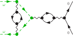
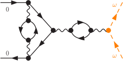
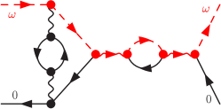
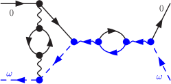
Figure 20: (Color online) A set of four diagrams for $\Gamma_{\uparrow\uparrow;\uparrow\uparrow}^{(4C)}$ contribution of which is given in Eq. (136).

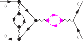
Figure 21: (Color online) Schematic picture for the total contribution $\widehat{\partial}_{i\omega}^{+}\Gamma_{\uparrow\uparrow;\uparrow\uparrow}^{(4C)}$ of the set shown in Fig. 20.

Total contribution of the diagrams shown in Fig. 20 can be rewritten in a total derivative form with respect to the loop frequency (see also Fig. 21):

$$\!\!\!\!\!\!\widehat{\partial}_{i\omega}^{+}\Gamma_{\uparrow\uparrow;\uparrow\uparrow}^{(4C)}(i\omega,0;0,i\omega)$$

$$=U^{4}\!\int_{-\infty}^{\infty}\!\int_{-\infty}^{\infty}\!\frac{d\varepsilon\,d\varepsilon^{\prime}}{(2\pi)^{2}}\ \chi_{\downarrow\downarrow}^{qp}(i\varepsilon)\ \widehat{\partial}_{i\omega}^{+}\,\biggl{[}\,-\,{\color[rgb]{1,0,0}G_{\uparrow}(i\varepsilon+i\omega)\,}\,G_{\uparrow}(i\varepsilon)\,{\color[rgb]{1,0,0}G_{\downarrow}(i\varepsilon^{\prime}+i\omega)\,}G_{\downarrow}(i\varepsilon^{\prime})\,\,-\,G_{\uparrow}(i\varepsilon)\,{\color[rgb]{0,0,1}G_{\uparrow}(i\varepsilon+i\omega)}\,G_{\downarrow}(i\varepsilon^{\prime}){\color[rgb]{0,0,1}G_{\downarrow}(i\varepsilon^{\prime}+i\omega)\,}\,$$

$$\qquad\qquad\qquad\qquad\qquad\qquad\qquad\qquad+{\color[rgb]{0,0.5,0}\left\{G_{\uparrow}(i\varepsilon+i\omega)\right\}^{2}\,}\left\{G_{\downarrow}(i\varepsilon^{\prime})\right\}^{2}\,+\left\{G_{\uparrow}(i\varepsilon)\right\}^{2}\,\left\{G_{\downarrow}(i\varepsilon^{\prime})\right\}^{2}\,\biggr{]}$$

$$= \ -U^{4}\!\int_{-\infty}^{\infty}\!\frac{d\varepsilon}{2\pi}\ \chi_{\downarrow\downarrow}^{qp}(i\varepsilon)\ \left\{G_{\uparrow}(i\varepsilon)\right\}^{2}\int_{-\infty}^{\infty}\!\frac{d\varepsilon^{\prime}}{2\pi}\ \widehat{\partial}_{i\omega}^{+}\,\biggl{[}\,{\color[rgb]{1,0,0}G_{\downarrow}(i\varepsilon^{\prime}+i\omega)\,}G_{\downarrow}(i\varepsilon^{\prime})\,+G_{\downarrow}(i\varepsilon^{\prime})\,{\color[rgb]{0,0,1}G_{\downarrow}(i\varepsilon^{\prime}+i\omega)\,}\,\biggr{]}$$

$$= \ -U^{4}\!\int_{-\infty}^{\infty}\!\frac{d\varepsilon}{2\pi}\ \chi_{\downarrow\downarrow}^{qp}(i\varepsilon)\ \left\{G_{\uparrow}(i\varepsilon)\right\}^{2}{\color[rgb]{1,0,1}\widehat{\partial}_{i\omega}^{+}\,\left[\,\int_{-\infty}^{\infty}\!\frac{d\varepsilon^{\prime}}{2\pi}\ \left\{G_{\downarrow}(i\varepsilon^{\prime}+i\omega)\right\}^{2}\,\,\right]}\ =\ 0.$$ (136)

Here, $U^{2}\chi_{\downarrow\downarrow}^{qp}(i\varepsilon)$ due to the particle-hole pair in the vertical direction can be regarded as a vertex correction between the external lines on the left side.

 

 

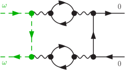
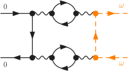
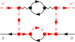
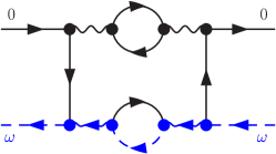
Figure 22: (Color online) A set of four diagrams for $\Gamma_{\uparrow\uparrow;\uparrow\uparrow}^{(4D)}$, contribution of which is given in Eq. (137).

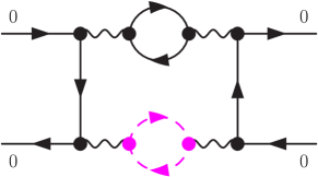
Figure 23: (Color online) Schematic picture for the total contribution $\widehat{\partial}_{i\omega}^{+}\Gamma_{\uparrow\uparrow;\uparrow\uparrow}^{(4D)}$ of the set shown in Fig. 22. The dashed propagators carrying the external frequency $\omega$ form a closed loop.

Total contribution of the diagrams shown in Fig. 22 can be rewritten in a total derivative form (see also Fig. 23):

$$\!\!\!\!\!\!\!\!\!\widehat{\partial}_{i\omega}^{+}\Gamma_{\uparrow\uparrow;\uparrow\uparrow}^{(4D)}(i\omega,0;0,i\omega)$$

$$=\,\frac{U^{4}}{2}\int_{-\infty}^{\infty}\frac{d\varepsilon}{2\pi}\ \widehat{\partial}_{i\omega}^{+}\biggl{[}\,{\color[rgb]{1,0,0}\chi_{\downarrow\downarrow}^{qp}(i\varepsilon+i\omega)}\,\chi_{\downarrow\downarrow}^{qp}(i\varepsilon)\,{\color[rgb]{1,0,0}\left\{G_{\uparrow}(i\varepsilon+i\omega)\right\}^{2}}+{\color[rgb]{0,0,1}\chi_{\downarrow\downarrow}^{qp}(i\varepsilon-i\omega)}\,\chi_{\downarrow\downarrow}^{qp}(i\varepsilon)\,{\color[rgb]{0,0,1}\left\{G_{\uparrow}(i\varepsilon)\right\}^{2}}$$

$$\qquad\qquad\qquad\qquad\quad-\left\{\chi_{\downarrow\downarrow}^{qp}(i\varepsilon)\right\}^{2}{\color[rgb]{0,0.5,0}G_{\uparrow}(i\varepsilon+i\omega)\,}G_{\uparrow}(i\varepsilon)\,-\left\{\chi_{\downarrow\downarrow}^{qp}(i\varepsilon)\right\}^{2}G_{\uparrow}(i\varepsilon)\,{\color[rgb]{1,0.5,0}G_{\uparrow}(i\varepsilon+i\omega)\,}\biggr{]}$$

$$=\,\frac{U^{4}}{2}\int_{-\infty}^{\infty}\frac{d\varepsilon}{2\pi}\,\left\{G_{\uparrow}(i\varepsilon)\right\}^{2}\widehat{\partial}_{i\omega}^{+}\left[\,{\color[rgb]{1,0,0}\chi_{\downarrow\downarrow}^{qp}(i\varepsilon+i\omega)}\,\chi_{\downarrow\downarrow}^{qp}(i\varepsilon)\,+{\color[rgb]{0,0,1}\chi_{\downarrow\downarrow}^{qp}(i\varepsilon-i\omega)}\,\chi_{\downarrow\downarrow}^{qp}(i\varepsilon)\,-2\left\{\chi_{\downarrow\downarrow}^{qp}(i\varepsilon)\right\}^{2}\right]$$

$$=\,-\,\frac{U^{4}}{2}\int_{-\infty}^{\infty}\frac{d\varepsilon}{2\pi}\,\left\{G_{\uparrow}(i\varepsilon)\right\}^{2}\chi_{\downarrow\downarrow}^{qp}(i\varepsilon)\,\int_{-\infty}^{\infty}\frac{d\varepsilon^{\prime}}{2\pi}\ \widehat{\partial}_{i\omega}^{+}\biggl{[}\,{\color[rgb]{1,0,0}G_{\downarrow}(i\varepsilon^{\prime}+i\varepsilon+i\omega)\,}G_{\downarrow}(i\varepsilon^{\prime})\,+G_{\downarrow}(i\varepsilon^{\prime}+i\varepsilon)\,{\color[rgb]{0,0,1}G_{\downarrow}(i\varepsilon^{\prime}+i\omega)\,}\,\biggr{]}$$

$$=\,-\,\frac{U^{4}}{2}\int_{-\infty}^{\infty}\frac{d\varepsilon}{2\pi}\,\left\{G_{\uparrow}(i\varepsilon)\right\}^{2}\chi_{\downarrow\downarrow}^{qp}(i\varepsilon)\ {\color[rgb]{1,0,1}\widehat{\partial}_{i\omega}^{+}\left[\,\int_{-\infty}^{\infty}\frac{d\varepsilon^{\prime}}{2\pi}\,G_{\downarrow}(i\varepsilon^{\prime}+i\varepsilon+i\omega)\,G_{\downarrow}(i\varepsilon^{\prime}+i\omega)\,\,\right]}\ =\ 0.$$ (137)

This set contains one singular particle-hole product $G_{\uparrow}(i\varepsilon+i\omega)G_{\uparrow}(i\varepsilon)$ carrying the same spin $\uparrow$ as that of the external one. The contribution of this product in the upper two diagrams of Fig. 22 and the contribution of the corresponding internal lines in the lower panel cancel each other out in the second line of Eq. (137), using the generalized chain rule for $\widehat{\partial}_{i\omega}^{+}$.

 

 

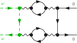
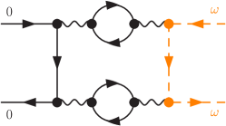
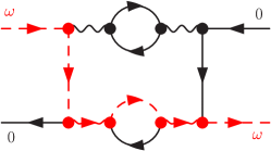
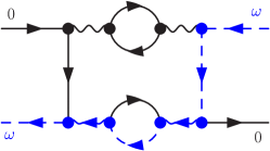
Figure 24: (Color online) A set of four diagrams for $\Gamma_{\uparrow\uparrow;\uparrow\uparrow}^{(4E)}$, contribution of which is given in Eq. (138).

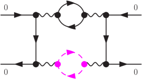
Figure 25: (Color online) Schematic picture for the total contribution $\widehat{\partial}_{i\omega}^{+}\Gamma_{\uparrow\uparrow;\uparrow\uparrow}^{(4E)}$ of the set shown in Fig. 24.

Next one is a set of diagrams that include the particle-particle pair. Specifically, this is the simplest example that the crossing symmetry cancels the singularity caused by the particle-particle pair excitation, described in Eq. (90). Total contribution of the diagrams shown in Fig. 24 can be rewritten in a total derivative form (see also Fig. 25):

$$\!\!\!\!\!\!\!\!\!\!\widehat{\partial}_{i\omega}^{+}\Gamma_{\uparrow\uparrow;\uparrow\uparrow}^{(4E)}(i\omega,0;0,i\omega)$$

$$=\,\frac{U^{4}}{2}\int_{-\infty}^{\infty}\frac{d\varepsilon}{2\pi}\ \widehat{\partial}_{i\omega}^{+}\biggl{[}\,{\color[rgb]{1,0,0}\chi_{\downarrow\downarrow}^{qp}(i\varepsilon+i\omega)}\,\chi_{\downarrow\downarrow}^{qp}(i\varepsilon)\,{\color[rgb]{1,0,0}G_{\uparrow}(i\varepsilon+i\omega)}\,G_{\uparrow}(-i\varepsilon)+{\color[rgb]{0,0,1}\chi_{\downarrow\downarrow}^{qp}(i\varepsilon-i\omega)}\,\chi_{\downarrow\downarrow}^{qp}(i\varepsilon)\,G_{\uparrow}(i\varepsilon)\,{\color[rgb]{0,0,1}G_{\uparrow}(i\omega-i\varepsilon)}$$

$$\qquad\qquad\qquad\qquad\quad-\left\{\chi_{\downarrow\downarrow}^{qp}(i\varepsilon)\right\}^{2}{\color[rgb]{0,0.5,0}G_{\uparrow}(i\varepsilon+i\omega)\,}G_{\uparrow}(-i\varepsilon)\,-\left\{\chi_{\downarrow\downarrow}^{qp}(i\varepsilon)\right\}^{2}G_{\uparrow}(i\varepsilon)\,{\color[rgb]{1,0.5,0}G_{\uparrow}(i\omega-i\varepsilon)\,}\biggr{]}$$

$$=\,\frac{U^{4}}{2}\int_{-\infty}^{\infty}\frac{d\varepsilon}{2\pi}\,G_{\uparrow}(i\varepsilon)\,G_{\uparrow}(-i\varepsilon)\ \widehat{\partial}_{i\omega}^{+}\left[\,{\color[rgb]{1,0,0}\chi_{\downarrow\downarrow}^{qp}(i\varepsilon+i\omega)}\,\chi_{\downarrow\downarrow}^{qp}(i\varepsilon)\,+{\color[rgb]{0,0,1}\chi_{\downarrow\downarrow}^{qp}(i\varepsilon-i\omega)}\,\chi_{\downarrow\downarrow}^{qp}(i\varepsilon)\,-2\left\{\chi_{\downarrow\downarrow}^{qp}(i\varepsilon)\right\}^{2}\right]$$

$$=\,-\,\frac{U^{4}}{2}\int_{-\infty}^{\infty}\frac{d\varepsilon}{2\pi}\,G_{\uparrow}(i\varepsilon)\,G_{\uparrow}(-i\varepsilon)\,\chi_{\downarrow\downarrow}^{qp}(i\varepsilon)\,\int_{-\infty}^{\infty}\frac{d\varepsilon^{\prime}}{2\pi}\ \widehat{\partial}_{i\omega}^{+}\biggl{[}\,{\color[rgb]{1,0,0}G_{\downarrow}(i\varepsilon^{\prime}+i\varepsilon+i\omega)\,}G_{\downarrow}(i\varepsilon^{\prime})\,+G_{\downarrow}(i\varepsilon^{\prime}+i\varepsilon)\,{\color[rgb]{0,0,1}G_{\downarrow}(i\varepsilon^{\prime}+i\omega)\,}\,\biggr{]}$$

$$=\,-\,\frac{U^{4}}{2}\int_{-\infty}^{\infty}\frac{d\varepsilon}{2\pi}\,G_{\uparrow}(i\varepsilon)\,G_{\uparrow}(-i\varepsilon)\,\chi_{\downarrow\downarrow}^{qp}(i\varepsilon)\ {\color[rgb]{1,0,1}\widehat{\partial}_{i\omega}^{+}\left[\,\int_{-\infty}^{\infty}\frac{d\varepsilon^{\prime}}{2\pi}\,G_{\downarrow}(i\varepsilon^{\prime}+i\varepsilon+i\omega)\,G_{\downarrow}(i\varepsilon^{\prime}+i\omega)\,\,\right]}\ =\ 0.$$ (138)

This set contains one singular particle-particle product, $G_{\uparrow}(i\varepsilon+i\omega)G_{\uparrow}(-i\varepsilon)$, or $G_{\uparrow}(i\varepsilon)G_{\uparrow}(i\omega-i\varepsilon)$, carrying the same spin $\uparrow$ as that of the external one. The contribution of this product in the upper two diagrams of Fig. 24 and those in the lower panel cancel each other out in the second line of Eq. (138), using the generalized chain rule for $\widehat{\partial}_{i\omega}^{+}$.

 

 

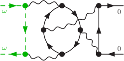
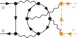
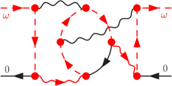
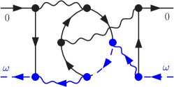
Figure 26: (Color online) A set of four diagrams for $\Gamma_{\uparrow\uparrow;\uparrow\uparrow}^{(4F)}$, contribution of which is given in Eq. (139).

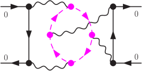
Figure 27: (Color online) Schematic picture for the total contribution $\widehat{\partial}_{i\omega}^{+}\Gamma_{\uparrow\uparrow;\uparrow\uparrow}^{(4F)}$ of the set shown in Fig. 26.

Total contribution of the diagrams shown in Fig. 26 can be rewritten in a total derivative form (see also Fig. 27):

$$\!\!\!\!\!\widehat{\partial}_{i\omega}^{+}\Gamma_{\uparrow\uparrow;\uparrow\uparrow}^{(4F)}(i\omega,0;0,i\omega)$$

$$=\,-U^{4}\int_{-\infty}^{\infty}\!\int_{-\infty}^{\infty}\!\int_{-\infty}^{\infty}\!\frac{d\varepsilon\,d\varepsilon_{1}\,d\varepsilon_{2}}{(2\pi)^{3}}\ \widehat{\partial}_{i\omega}^{+}\biggl{[}\,G_{\uparrow}(i\varepsilon_{1})\,G_{\downarrow}(i\varepsilon_{1}+i\varepsilon)\,G_{\downarrow}(i\varepsilon_{1}+i\varepsilon_{2}+i\varepsilon)\,{\color[rgb]{0,0,1}G_{\downarrow}(i\varepsilon+i\omega)\,}G_{\downarrow}(i\varepsilon_{2}+i\varepsilon)\,G_{\uparrow}(i\varepsilon_{2})\,$$

$$\qquad\qquad\qquad+{\color[rgb]{1,0,0}G_{\uparrow}(i\varepsilon_{1}+i\omega)\,G_{\downarrow}(i\varepsilon_{1}+i\varepsilon+i\omega)\,G_{\downarrow}(i\varepsilon_{1}+i\varepsilon_{2}+i\varepsilon+i\omega)\,}G_{\downarrow}(i\varepsilon)\,{\color[rgb]{1,0,0}G_{\downarrow}(i\varepsilon_{2}+i\varepsilon+i\omega)\,G_{\uparrow}(i\varepsilon_{2}+i\omega)\,}$$

$$\qquad\qquad\qquad-{\color[rgb]{0,0.5,0}G_{\uparrow}(i\varepsilon_{1}+i\omega)\,}G_{\downarrow}(i\varepsilon_{1}+i\varepsilon)\,G_{\downarrow}(i\varepsilon+i\varepsilon_{1}+i\varepsilon_{2})\,G_{\downarrow}(i\varepsilon)\,G_{\downarrow}(i\varepsilon_{2}+i\varepsilon)\,G_{\uparrow}(i\varepsilon_{2})\,$$

$$\qquad\qquad\qquad-G_{\uparrow}(i\varepsilon_{1})\,G_{\downarrow}(i\varepsilon_{1}+i\varepsilon)\,G_{\downarrow}(i\varepsilon+i\varepsilon_{1}+i\varepsilon_{2})\,G_{\downarrow}(i\varepsilon)\,G_{\downarrow}(i\varepsilon_{2}+i\varepsilon)\,{\color[rgb]{1,0.5,0}G_{\uparrow}(i\varepsilon_{2}+i\omega)\,}\,\biggr{]}$$

$$=\ -U^{4}\int_{-\infty}^{\infty}\!\int_{-\infty}^{\infty}\!\frac{d\varepsilon_{1}\,d\varepsilon_{2}}{(2\pi)^{2}}\ G_{\uparrow}(i\varepsilon_{1})\,G_{\uparrow}(i\varepsilon_{2})\int_{-\infty}^{\infty}\!\frac{d\varepsilon}{2\pi}\ \widehat{\partial}_{i\omega}^{+}\biggl{[}\,G_{\downarrow}(i\varepsilon_{1}+i\varepsilon)\,G_{\downarrow}(i\varepsilon+i\varepsilon_{1}+i\varepsilon_{2})\,{\color[rgb]{0,0,1}G_{\downarrow}(i\varepsilon+i\omega)\,}G_{\downarrow}(i\varepsilon_{2}+i\varepsilon)\,$$

$$+{\color[rgb]{1,0,0}G_{\downarrow}(i\varepsilon_{1}+i\varepsilon+i\omega)\,G_{\downarrow}(i\varepsilon_{1}+i\varepsilon_{2}+i\varepsilon+i\omega)\,}G_{\downarrow}(i\varepsilon)\,{\color[rgb]{1,0,0}G_{\downarrow}(i\varepsilon_{2}+i\varepsilon+i\omega)\,}-2G_{\downarrow}(i\varepsilon_{1}+i\varepsilon)\,G_{\downarrow}(i\varepsilon+i\varepsilon_{1}+i\varepsilon_{2})\,G_{\downarrow}(i\varepsilon)\,G_{\downarrow}(i\varepsilon_{2}+i\varepsilon)\,\,\biggr{]}$$

$$=-U^{4}\!\!\int_{-\infty}^{\infty}\!\!\int_{-\infty}^{\infty}\!\!\frac{d\varepsilon_{1}d\varepsilon_{2}}{(2\pi)^{2}}\,G_{\uparrow}(i\varepsilon_{1})\,G_{\uparrow}(i\varepsilon_{2})\ {\color[rgb]{1,0,1}\widehat{\partial}_{i\omega}^{+}\left[\int_{-\infty}^{\infty}\!\!\frac{d\varepsilon}{2\pi}\ G_{\downarrow}(i\varepsilon_{1}+i\varepsilon+i\omega)\,G_{\downarrow}(i\varepsilon+i\varepsilon_{1}+i\varepsilon_{2}+i\omega)\,G_{\downarrow}(i\varepsilon+i\omega)\,G_{\downarrow}(i\varepsilon_{2}+i\varepsilon+i\omega)\,\right]}$$

$$=\ 0\;.$$ (139)

The diagram of this set cannot be separated into two parts by cutting two internal lines, and thus it has no singular Green’s-function product. To obtain the second line, the derivative with respect to $\widehat{\partial}_{i\omega}^{+}$ is taken for $\omega$’s which are assigned for the $\uparrow$ spin propagators in the vertical direction. Then, the remaining contribution arising from the two diagrams in the lower panel of Fig. 26 is extracted to obtain the third line of Eq. (139).

 

 

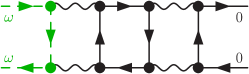
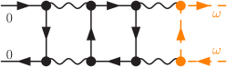
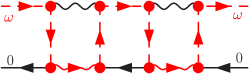
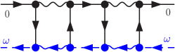
Figure 28: (Color online) A set of four diagrams for $\Gamma_{\uparrow\uparrow;\uparrow\uparrow}^{(4G)}$, contribution of which is given in Eq. (140).

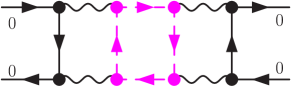
Figure 29: (Color online) Schematic picture for the total contribution $\widehat{\partial}_{i\omega}^{+}\Gamma_{\uparrow\uparrow;\uparrow\uparrow}^{(4G)}$. of the set shown in Fig. 28.

Total contribution of the diagrams shown in Fig. 28 can be rewritten in a total derivative form (see also Fig. 29):

$$\!\!\!\!\!\widehat{\partial}_{i\omega}^{+}\Gamma_{\uparrow\uparrow;\uparrow\uparrow}^{(4G)}(i\omega,0;0,i\omega)$$

$$=\,-\frac{U^{4}}{2}\int_{-\infty}^{\infty}\!\int_{-\infty}^{\infty}\!\int_{-\infty}^{\infty}\!\frac{d\varepsilon\,d\varepsilon_{1}\,d\varepsilon_{2}}{(2\pi)^{3}}\ \widehat{\partial}_{i\omega}^{+}\biggl{[}\,G_{\uparrow}(i\varepsilon_{1})\,G_{\downarrow}(i\varepsilon_{1}+i\varepsilon)\,G_{\downarrow}(i\varepsilon)\,{\color[rgb]{0,0,1}G_{\downarrow}(i\varepsilon+i\omega)\,}G_{\downarrow}(i\varepsilon_{2}+i\varepsilon)\,G_{\uparrow}(i\varepsilon_{2})\,$$

$$\qquad\qquad\qquad+{\color[rgb]{1,0,0}G_{\uparrow}(i\varepsilon_{1}+i\omega)\,G_{\downarrow}(i\varepsilon_{1}+i\varepsilon+i\omega)\,G_{\downarrow}(i\varepsilon+i\omega)\,}G_{\downarrow}(i\varepsilon)\,{\color[rgb]{1,0,0}G_{\downarrow}(i\varepsilon_{2}+i\varepsilon+i\omega)\,G_{\uparrow}(i\varepsilon_{2}+i\omega)\,}$$

$$\qquad\qquad\qquad-{\color[rgb]{0,0.5,0}G_{\uparrow}(i\varepsilon_{1}+i\omega)\,}G_{\downarrow}(i\varepsilon_{1}+i\varepsilon)\,\left\{G_{\downarrow}(i\varepsilon)\right\}^{2}\,G_{\downarrow}(i\varepsilon_{2}+i\varepsilon)\,G_{\uparrow}(i\varepsilon_{2})\,$$

$$\qquad\qquad\qquad-G_{\uparrow}(i\varepsilon_{1})\,G_{\downarrow}(i\varepsilon_{1}+i\varepsilon)\,\left\{G_{\downarrow}(i\varepsilon)\right\}^{2}\,G_{\downarrow}(i\varepsilon_{2}+i\varepsilon)\,{\color[rgb]{1,0.5,0}G_{\uparrow}(i\varepsilon_{2}+i\omega)\,}\,\biggr{]}$$

$$=\ -\frac{U^{4}}{2}\int_{-\infty}^{\infty}\!\int_{-\infty}^{\infty}\!\frac{d\varepsilon_{1}\,d\varepsilon_{2}}{(2\pi)^{2}}\ G_{\uparrow}(i\varepsilon_{1})\,G_{\uparrow}(i\varepsilon_{2})\int_{-\infty}^{\infty}\!\frac{d\varepsilon}{2\pi}\ \widehat{\partial}_{i\omega}^{+}\biggl{[}\,G_{\downarrow}(i\varepsilon_{1}+i\varepsilon)\,G_{\downarrow}(i\varepsilon)\,{\color[rgb]{0,0,1}G_{\downarrow}(i\varepsilon+i\omega)\,}G_{\downarrow}(i\varepsilon_{2}+i\varepsilon)\,$$

$$\qquad\qquad+{\color[rgb]{1,0,0}G_{\downarrow}(i\varepsilon_{1}+i\varepsilon+i\omega)\,G_{\downarrow}(i\varepsilon+i\omega)\,}G_{\downarrow}(i\varepsilon)\,{\color[rgb]{1,0,0}G_{\downarrow}(i\varepsilon_{2}+i\varepsilon+i\omega)\,}-2G_{\downarrow}(i\varepsilon_{1}+i\varepsilon)\,\left\{G_{\downarrow}(i\varepsilon)\right\}^{2}\,G_{\downarrow}(i\varepsilon_{2}+i\varepsilon)\,\,\biggr{]}$$

$$=\ -\frac{U^{4}}{2}\int_{-\infty}^{\infty}\!\int_{-\infty}^{\infty}\!\frac{d\varepsilon_{1}\,d\varepsilon_{2}}{(2\pi)^{2}}\ G_{\uparrow}(i\varepsilon_{1})\,G_{\uparrow}(i\varepsilon_{2})\ {\color[rgb]{1,0,1}\widehat{\partial}_{i\omega}^{+}\left[\,\int_{-\infty}^{\infty}\!\frac{d\varepsilon}{2\pi}\ G_{\downarrow}(i\varepsilon_{1}+i\varepsilon+i\omega)\,\left\{G_{\downarrow}(i\varepsilon+i\omega)\right\}^{2}\,G_{\downarrow}(i\varepsilon_{2}+i\varepsilon+i\omega)\,\right]}$$

$$=\ 0\;.$$ (140)

This set contains one singular particle-hole pair $G_{\downarrow}(i\varepsilon)G_{\downarrow}(i\varepsilon+i\omega)$ carrying $\omega$ in the horizontal direction. To obtain the second line, the derivative with respect to $\widehat{\partial}_{i\omega}^{+}$ is taken for $\omega$’s which are assigned for the $\uparrow$ spin propagators in the vertical direction. Then, the remaining contribution arising from the two diagrams in the lower panel of Fig. 28 is extracted to obtain the third line of Eq. (140).

 

 

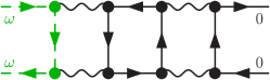
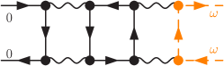
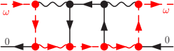
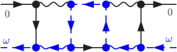
Figure 30: (Color online) A set of four diagrams for $\Gamma_{\uparrow\uparrow;\uparrow\uparrow}^{(4H)}$, contribution of which is given in Eq. (141).

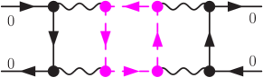
Figure 31: (Color online) Sum of the derivative $\widehat{\partial}_{i\omega}^{+}\Gamma_{\uparrow\uparrow;\uparrow\uparrow}^{(4H)}$ and the related other three. Schematic picture for the total contribution $\widehat{\partial}_{i\omega}^{+}\Gamma_{\uparrow\uparrow;\uparrow\uparrow}^{(4H)}$ of the set shown in Fig. 30.

Total contribution of the diagrams shown in Fig. 30 can be rewritten in a total derivative form (see also Fig. 31):

$$\!\!\!\!\!\widehat{\partial}_{i\omega}^{+}\Gamma_{\uparrow\uparrow;\uparrow\uparrow}^{(4H)}(i\omega,0;0,i\omega)$$

$$=\,-\frac{U^{4}}{2}\int_{-\infty}^{\infty}\!\int_{-\infty}^{\infty}\!\int_{-\infty}^{\infty}\!\frac{d\varepsilon\,d\varepsilon_{1}\,d\varepsilon_{2}}{(2\pi)^{3}}\ \widehat{\partial}_{i\omega}^{+}\biggl{[}\,G_{\uparrow}(i\varepsilon_{1})\,G_{\downarrow}(i\varepsilon)\,{\color[rgb]{0,0,1}G_{\downarrow}(i\varepsilon-i\varepsilon_{1}+i\omega)\,G_{\downarrow}(i\varepsilon+i\omega)\,G_{\downarrow}(i\varepsilon-i\varepsilon_{2}+i\omega)\,}G_{\uparrow}(i\varepsilon_{2})\,$$

$$\qquad\qquad\qquad+{\color[rgb]{1,0,0}G_{\uparrow}(i\varepsilon_{1}+i\omega)\,G_{\downarrow}(i\varepsilon+i\omega)\,}G_{\downarrow}(i\varepsilon-i\varepsilon_{1})\,G_{\downarrow}(i\varepsilon)\,G_{\downarrow}(i\varepsilon-\varepsilon_{2})\,{\color[rgb]{1,0,0}G_{\uparrow}(i\varepsilon_{2}+i\omega)\,}$$

$$\qquad\qquad\qquad-{\color[rgb]{0,0.5,0}G_{\uparrow}(i\varepsilon_{1}+i\omega)\,}G_{\downarrow}(i\varepsilon-i\varepsilon_{1})\,\left\{G_{\downarrow}(i\varepsilon)\right\}^{2}\,G_{\downarrow}(i\varepsilon-i\varepsilon_{2})\,G_{\uparrow}(i\varepsilon_{2})\,$$

$$\qquad\qquad\qquad-G_{\uparrow}(i\varepsilon_{1})\,G_{\downarrow}(i\varepsilon-i\varepsilon_{1})\,\left\{G_{\downarrow}(i\varepsilon)\right\}^{2}\,G_{\downarrow}(i\varepsilon-i\varepsilon_{2})\,{\color[rgb]{1,0.5,0}G_{\uparrow}(i\varepsilon_{2}+i\omega)\,}\,\biggr{]}$$

$$=\ -\frac{U^{4}}{2}\int_{-\infty}^{\infty}\!\int_{-\infty}^{\infty}\!\frac{d\varepsilon_{1}\,d\varepsilon_{2}}{(2\pi)^{2}}\ G_{\uparrow}(i\varepsilon_{1})\,G_{\uparrow}(i\varepsilon_{2})\int_{-\infty}^{\infty}\!\frac{d\varepsilon}{2\pi}\ \widehat{\partial}_{i\omega}^{+}\biggl{[}\,G_{\downarrow}(i\varepsilon)\,{\color[rgb]{0,0,1}G_{\downarrow}(i\varepsilon-i\varepsilon_{1}+i\omega)\,G_{\downarrow}(i\varepsilon+i\omega)\,G_{\downarrow}(i\varepsilon-i\varepsilon_{2}+i\omega)\,}$$

$$\qquad\qquad+{\color[rgb]{1,0,0}G_{\downarrow}(i\varepsilon+i\omega)\,}G_{\downarrow}(i\varepsilon-i\varepsilon_{1})\,G_{\downarrow}(i\varepsilon)\,G_{\downarrow}(i\varepsilon-i\varepsilon_{2})\,-2G_{\downarrow}(i\varepsilon-i\varepsilon_{1})\,\left\{G_{\downarrow}(i\varepsilon)\right\}^{2}\,G_{\downarrow}(i\varepsilon-i\varepsilon_{2})\,\,\biggr{]}$$

$$=\ -\frac{U^{4}}{2}\int_{-\infty}^{\infty}\!\int_{-\infty}^{\infty}\!\frac{d\varepsilon_{1}\,d\varepsilon_{2}}{(2\pi)^{2}}\ G_{\uparrow}(i\varepsilon_{1})\,G_{\uparrow}(i\varepsilon_{2})\ {\color[rgb]{1,0,1}\widehat{\partial}_{i\omega}^{+}\left[\,\int_{-\infty}^{\infty}\!\frac{d\varepsilon}{2\pi}\ G_{\downarrow}(i\varepsilon-i\varepsilon_{1}+i\omega)\,\left\{G_{\downarrow}(i\varepsilon+i\omega)\right\}^{2}\,G_{\downarrow}(i\varepsilon-i\varepsilon_{2}+i\omega)\,\right]}$$

$$=\ 0\;.$$ (141)

This set also contains one singular particle-hole pair $G_{\downarrow}(i\varepsilon)G_{\downarrow}(i\varepsilon+i\omega)$ carrying $\omega$ in the horizontal direction. To obtain the second line, the derivative with respect to $\widehat{\partial}_{i\omega}^{+}$ is taken for $\omega$’s which are assigned for the $\uparrow$ spin propagators in the vertical direction. Then, the remaining contribution arising from the two diagrams in the lower panel of Fig. 30 is extracted to obtain the third line of Eq. (141).

 

 

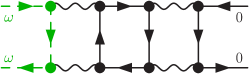
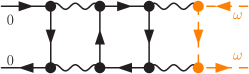
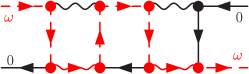
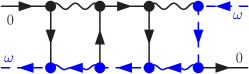
Figure 32: (Color online) A set of four diagrams for $\Gamma_{\uparrow\uparrow;\uparrow\uparrow}^{(4I)}$, contribution of which is given in Eq. (142).

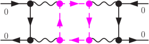
Figure 33: (Color online) Schematic picture for the total contribution $\widehat{\partial}_{i\omega}^{+}\Gamma_{\uparrow\uparrow;\uparrow\uparrow}^{(4I)}$ of the set shown in Fig. 32

Total contribution of the diagrams shown in Fig. 32 can be rewritten in a total derivative form (see also Fig. 33):

$$\!\!\!\!\!\widehat{\partial}_{i\omega}^{+}\Gamma_{\uparrow\uparrow;\uparrow\uparrow}^{(4I)}(i\omega,0;0,i\omega)$$

$$=\,-U^{4}\int_{-\infty}^{\infty}\!\int_{-\infty}^{\infty}\!\int_{-\infty}^{\infty}\!\frac{d\varepsilon\,d\varepsilon_{1}\,d\varepsilon_{2}}{(2\pi)^{3}}\ \widehat{\partial}_{i\omega}^{+}\biggl{[}\,G_{\uparrow}(i\varepsilon_{1})\,G_{\downarrow}(i\varepsilon)\,G_{\downarrow}(i\varepsilon+i\varepsilon_{1})\,G_{\downarrow}(i\varepsilon-i\varepsilon_{2})\,{\color[rgb]{0,0,1}G_{\downarrow}(i\varepsilon+i\omega)\,G_{\uparrow}(i\varepsilon_{2}+i\omega)\,}$$

$$\qquad\qquad\qquad+{\color[rgb]{1,0,0}G_{\uparrow}(i\varepsilon_{1}+i\omega)\,G_{\downarrow}(i\varepsilon+i\omega)\,G_{\downarrow}(i\varepsilon+i\varepsilon_{1}+i\omega)\,G_{\downarrow}(i\varepsilon-\varepsilon_{2}+i\omega)\,}G_{\downarrow}(i\varepsilon)\,G_{\uparrow}(i\varepsilon_{2})\,$$

$$\qquad\qquad\qquad-{\color[rgb]{0,0.5,0}G_{\uparrow}(i\varepsilon_{1}+i\omega)\,}G_{\downarrow}(i\varepsilon+i\varepsilon_{1})\,G_{\downarrow}(i\varepsilon-i\varepsilon_{2})\,\left\{G_{\downarrow}(i\varepsilon)\right\}^{2}\,G_{\uparrow}(i\varepsilon_{2})\,$$

$$\qquad\qquad\qquad-G_{\uparrow}(i\varepsilon_{1})\,G_{\downarrow}(i\varepsilon+i\varepsilon_{1})\,G_{\downarrow}(i\varepsilon-i\varepsilon_{2})\,\left\{G_{\downarrow}(i\varepsilon)\right\}^{2}\,{\color[rgb]{1,0.5,0}G_{\uparrow}(i\varepsilon_{2}+i\omega)\,}\,\biggr{]}$$

$$=\ -U^{4}\int_{-\infty}^{\infty}\!\int_{-\infty}^{\infty}\!\frac{d\varepsilon_{1}\,d\varepsilon_{2}}{(2\pi)^{2}}\ G_{\uparrow}(i\varepsilon_{1})\,G_{\uparrow}(i\varepsilon_{2})\int_{-\infty}^{\infty}\!\frac{d\varepsilon}{2\pi}\ \widehat{\partial}_{i\omega}^{+}\biggl{[}\,G_{\downarrow}(i\varepsilon)\,G_{\downarrow}(i\varepsilon+i\varepsilon_{1})\,G_{\downarrow}(i\varepsilon-i\varepsilon_{2})\,{\color[rgb]{0,0,1}G_{\downarrow}(i\varepsilon+i\omega)\,}$$

$$\qquad\qquad+{\color[rgb]{1,0,0}G_{\downarrow}(i\varepsilon+i\omega)\,G_{\downarrow}(i\varepsilon+i\varepsilon_{1}+i\omega)\,G_{\downarrow}(i\varepsilon-i\varepsilon_{2}+i\omega)\,}G_{\downarrow}(i\varepsilon)\,-2G_{\downarrow}(i\varepsilon+i\varepsilon_{1})\,\left\{G_{\downarrow}(i\varepsilon)\right\}^{2}\,G_{\downarrow}(i\varepsilon-i\varepsilon_{2})\,\,\biggr{]}$$

$$=\ -U^{4}\int_{-\infty}^{\infty}\!\int_{-\infty}^{\infty}\!\frac{d\varepsilon_{1}\,d\varepsilon_{2}}{(2\pi)^{2}}\ G_{\uparrow}(i\varepsilon_{1})\,G_{\uparrow}(i\varepsilon_{2})\ {\color[rgb]{1,0,1}\widehat{\partial}_{i\omega}^{+}\left[\,\int_{-\infty}^{\infty}\!\frac{d\varepsilon}{2\pi}\ G_{\downarrow}(i\varepsilon+i\varepsilon_{1}+i\omega)\,\left\{G_{\downarrow}(i\varepsilon+i\omega)\right\}^{2}\,G_{\downarrow}(i\varepsilon-i\varepsilon_{2}+i\omega)\,\right]}$$

$$=\ 0\;.$$ (142)

This set also contains one singular particle-hole pair $G_{\downarrow}(i\varepsilon)G_{\downarrow}(i\varepsilon+i\omega)$ carrying $\omega$ in the horizontal direction. To obtain the second line, the derivative with respect to $\widehat{\partial}_{i\omega}^{+}$ is taken for $\omega$’s which are assigned for the $\uparrow$ spin propagators in the vertical direction. Then, the remaining contribution arising from the two diagrams in the lower panel of Fig. 32 is extracted to obtain the third line of Eq. (142).

 

 

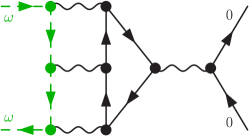
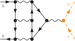
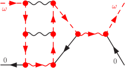
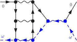
Figure 34: (Color online) A set of four diagrams for $\Gamma_{\uparrow\uparrow;\uparrow\uparrow}^{(4J)}$, contribution of which is given in Eq. (143).

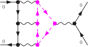
Figure 35: (Color online) Schematic picture for the total contribution $\widehat{\partial}_{i\omega}^{+}\Gamma_{\uparrow\uparrow;\uparrow\uparrow}^{(4J)}$ of the set shown in Fig. 34.

Total contribution of the diagrams shown in Fig. 34 can be rewritten in a total derivative form (see also Fig. 35):

$$\!\!\!\!\!\widehat{\partial}_{i\omega}^{+}\Gamma_{\uparrow\uparrow;\uparrow\uparrow}^{(4J)}(i\omega,0;0,i\omega)$$

$$=\,-U^{4}\int_{-\infty}^{\infty}\!\int_{-\infty}^{\infty}\!\int_{-\infty}^{\infty}\!\frac{d\varepsilon\,d\varepsilon_{1}\,d\varepsilon_{2}}{(2\pi)^{3}}\ \widehat{\partial}_{i\omega}^{+}\biggl{[}\,G_{\uparrow}(i\varepsilon_{1})\,G_{\uparrow}(i\varepsilon_{2})\,G_{\downarrow}(i\varepsilon+i\varepsilon_{1})\,G_{\downarrow}(i\varepsilon+i\varepsilon_{2})\,G_{\downarrow}(i\varepsilon)\,{\color[rgb]{0,0,1}G_{\downarrow}(i\varepsilon+i\omega)\,}$$

$$\qquad\qquad\qquad\qquad\qquad+{\color[rgb]{1,0,0}G_{\uparrow}(i\varepsilon_{1}+i\omega)\,G_{\uparrow}(i\varepsilon_{2}+i\omega)\,G_{\downarrow}(i\varepsilon+i\varepsilon_{1}+i\omega)\,G_{\downarrow}(i\varepsilon+i\varepsilon_{2}+i\omega)\,G_{\downarrow}(i\varepsilon+i\omega)}\,G_{\downarrow}(i\varepsilon)\,$$

$$\qquad\qquad\qquad\qquad\qquad-{\color[rgb]{0,0.5,0}G_{\uparrow}(i\varepsilon_{1}+i\omega)\,G_{\uparrow}(i\varepsilon_{2}+i\omega)\,}G_{\downarrow}(i\varepsilon+i\varepsilon_{1})\,G_{\downarrow}(i\varepsilon+i\varepsilon_{2})\,G_{\downarrow}(i\varepsilon)\,G_{\downarrow}(i\varepsilon)\,$$

$$\qquad\qquad\qquad\qquad\qquad-G_{\uparrow}(i\varepsilon_{1})\,G_{\uparrow}(i\varepsilon_{2})\,G_{\downarrow}(i\varepsilon+i\varepsilon_{1})\,G_{\downarrow}(i\varepsilon+i\varepsilon_{2})\,G_{\downarrow}(i\varepsilon)\,G_{\downarrow}(i\varepsilon)\,\,\biggr{]}$$

$$=\ -U^{4}\int_{-\infty}^{\infty}\!\int_{-\infty}^{\infty}\!\frac{d\varepsilon_{1}\,d\varepsilon_{2}}{(2\pi)^{2}}\ G_{\uparrow}(i\varepsilon_{1})\,G_{\uparrow}(i\varepsilon_{2})\int_{-\infty}^{\infty}\!\frac{d\varepsilon}{2\pi}\ \widehat{\partial}_{i\omega}^{+}\biggl{[}\,G_{\downarrow}(i\varepsilon+i\varepsilon_{1})\,G_{\downarrow}(i\varepsilon+i\varepsilon_{2})\,G_{\downarrow}(i\varepsilon)\,{\color[rgb]{0,0,1}G_{\downarrow}(i\varepsilon+i\omega)\,}$$

$$\qquad\qquad\qquad+{\color[rgb]{1,0,0}G_{\downarrow}(i\varepsilon+i\varepsilon_{1}+i\omega)\,G_{\downarrow}(i\varepsilon+i\varepsilon_{2}+i\omega)\,G_{\downarrow}(i\varepsilon+i\omega)}\,G_{\downarrow}(i\varepsilon)\,-2G_{\downarrow}(i\varepsilon+i\varepsilon_{1})\,G_{\downarrow}(i\varepsilon+i\varepsilon_{2})\,G_{\downarrow}(i\varepsilon)\,G_{\downarrow}(i\varepsilon)\,\,\,\biggr{]}$$

$$=-U^{4}\!\!\int_{-\infty}^{\infty}\!\!\int_{-\infty}^{\infty}\!\!\frac{d\varepsilon_{1}d\varepsilon_{2}}{(2\pi)^{2}}\,G_{\uparrow}(i\varepsilon_{1})\,G_{\uparrow}(i\varepsilon_{2})\ {\color[rgb]{1,0,1}\widehat{\partial}_{i\omega}^{+}\left[\int_{-\infty}^{\infty}\!\!\frac{d\varepsilon}{2\pi}\ G_{\downarrow}(i\varepsilon+i\varepsilon_{1}+i\omega)\,G_{\downarrow}(i\varepsilon+i\varepsilon_{2}+i\omega)\,\left\{G_{\downarrow}(i\varepsilon+i\omega)\right\}^{2}\,\right]}$$

$$=\ 0\;.$$ (143)

To obtain the second line, the derivative with respect to $\widehat{\partial}_{i\omega}^{+}$ is taken for $\omega$’s which are assigned for the $\uparrow$ spin propagators in the vertical direction. The remaining contribution arising from the two diagrams in the lower panel of Fig. 34 is extracted by applying the generalized chain rule for the product $G_{\downarrow}(i\varepsilon)G_{\downarrow}(i\varepsilon+i\omega)$.

 

 

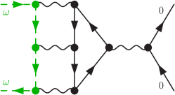
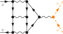
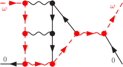
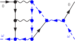
Figure 36: (Color online) A set of four diagrams for $\Gamma_{\uparrow\uparrow;\uparrow\uparrow}^{(4K)}$, contribution of which is given in Eq. (144).

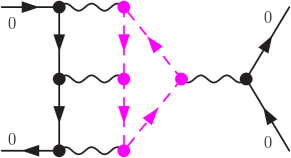
Figure 37: (Color online) Schematic picture for the total contribution $\widehat{\partial}_{i\omega}^{+}\Gamma_{\uparrow\uparrow;\uparrow\uparrow}^{(4K)}$ of the set shown in Fig. 36.

Total contribution of the diagrams shown in Fig. 36 can be rewritten in a total derivative form (see also Fig. 37):

$$\!\!\!\!\!\widehat{\partial}_{i\omega}^{+}\Gamma_{\uparrow\uparrow;\uparrow\uparrow}^{(4K)}(i\omega,0;0,i\omega)$$

$$=\,-U^{4}\int_{-\infty}^{\infty}\!\int_{-\infty}^{\infty}\!\int_{-\infty}^{\infty}\!\frac{d\varepsilon\,d\varepsilon_{1}\,d\varepsilon_{2}}{(2\pi)^{3}}\ \widehat{\partial}_{i\omega}^{+}\biggl{[}\,G_{\uparrow}(i\varepsilon_{1})\,G_{\uparrow}(i\varepsilon_{2})\,{\color[rgb]{0,0,1}G_{\downarrow}(i\varepsilon-i\varepsilon_{1}+i\omega)\,G_{\downarrow}(i\varepsilon-i\varepsilon_{2}+i\omega)\,G_{\downarrow}(i\varepsilon+i\omega)\,}G_{\downarrow}(i\varepsilon)\,$$

$$\qquad\qquad\qquad\qquad\qquad+{\color[rgb]{1,0,0}G_{\uparrow}(i\varepsilon_{1}+i\omega)\,G_{\uparrow}(i\varepsilon_{2}+i\omega)\,}G_{\downarrow}(i\varepsilon-i\varepsilon_{1})\,G_{\downarrow}(i\varepsilon-i\varepsilon_{2})\,G_{\downarrow}(i\varepsilon)\,{\color[rgb]{1,0,0}G_{\downarrow}(i\varepsilon+i\omega)\,}$$

$$\qquad\qquad\qquad\qquad\qquad-{\color[rgb]{0,0.5,0}G_{\uparrow}(i\varepsilon_{1}+i\omega)\,G_{\uparrow}(i\varepsilon_{2}+i\omega)\,}G_{\downarrow}(i\varepsilon-i\varepsilon_{1})\,G_{\downarrow}(i\varepsilon-i\varepsilon_{2})\,G_{\downarrow}(i\varepsilon)\,G_{\downarrow}(i\varepsilon)\,$$

$$\qquad\qquad\qquad\qquad\qquad-G_{\uparrow}(i\varepsilon_{1})\,G_{\uparrow}(i\varepsilon_{2})\,G_{\downarrow}(i\varepsilon-i\varepsilon_{1})\,G_{\downarrow}(i\varepsilon-i\varepsilon_{2})\,G_{\downarrow}(i\varepsilon)\,G_{\downarrow}(i\varepsilon)\,\,\biggr{]}$$

$$=\ -U^{4}\int_{-\infty}^{\infty}\!\int_{-\infty}^{\infty}\!\frac{d\varepsilon_{1}\,d\varepsilon_{2}}{(2\pi)^{2}}\ G_{\uparrow}(i\varepsilon_{1})\,G_{\uparrow}(i\varepsilon_{2})\int_{-\infty}^{\infty}\!\frac{d\varepsilon}{2\pi}\ \widehat{\partial}_{i\omega}^{+}\biggl{[}\,{\color[rgb]{0,0,1}G_{\downarrow}(i\varepsilon-i\varepsilon_{1}+i\omega)\,G_{\downarrow}(i\varepsilon-i\varepsilon_{2}+i\omega)\,G_{\downarrow}(i\varepsilon+i\omega)\,}G_{\downarrow}(i\varepsilon)\,$$

$$\qquad\qquad\qquad+G_{\downarrow}(i\varepsilon-i\varepsilon_{1})\,G_{\downarrow}(i\varepsilon-i\varepsilon_{2})\,G_{\downarrow}(i\varepsilon)\,{\color[rgb]{1,0,0}G_{\downarrow}(i\varepsilon+i\omega)\,}-2G_{\downarrow}(i\varepsilon-i\varepsilon_{1})\,G_{\downarrow}(i\varepsilon-i\varepsilon_{2})\,G_{\downarrow}(i\varepsilon)\,G_{\downarrow}(i\varepsilon)\,\,\biggr{]}$$

$$=-U^{4}\!\!\int_{-\infty}^{\infty}\!\!\int_{-\infty}^{\infty}\!\!\frac{d\varepsilon_{1}d\varepsilon_{2}}{(2\pi)^{2}}\,G_{\uparrow}(i\varepsilon_{1})\,G_{\uparrow}(i\varepsilon_{2})\ {\color[rgb]{1,0,1}\widehat{\partial}_{i\omega}^{+}\left[\int_{-\infty}^{\infty}\!\!\frac{d\varepsilon}{2\pi}\ G_{\downarrow}(i\varepsilon-i\varepsilon_{1}+i\omega)\,G_{\downarrow}(i\varepsilon-i\varepsilon_{2}+i\omega)\,\left\{G_{\downarrow}(i\varepsilon+i\omega)\right\}^{2}\,\right]}$$

$$=\ 0\;.$$ (144)

To obtain the second line, the derivative with respect to $\widehat{\partial}_{i\omega}^{+}$ is taken for $\omega$’s which are assigned for the $\uparrow$ spin propagators in the vertical direction. The remaining contribution arising from the two diagrams in the lower panel of Fig. 36 is extracted by applying the generalized chain rule for the product $G_{\downarrow}(i\varepsilon)G_{\downarrow}(i\varepsilon+i\omega)$.

 

 

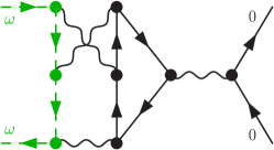
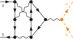
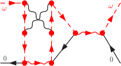
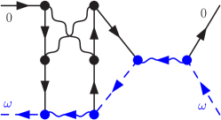
Figure 38: (Color online) A set of four diagrams for $\Gamma_{\uparrow\uparrow;\uparrow\uparrow}^{(4L)}$, contribution of which is given in Eq. (145).

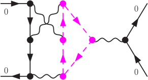
Figure 39: (Color online) Schematic picture for the total contribution $\widehat{\partial}_{i\omega}^{+}\Gamma_{\uparrow\uparrow;\uparrow\uparrow}^{(4L)}$ of the diagrams shown in Fig. 38.

Total contribution of the diagrams shown in Fig. 38 can be rewritten in a total derivative form (see also Fig. 39):

$$\!\!\!\!\!\widehat{\partial}_{i\omega}^{+}\Gamma_{\uparrow\uparrow;\uparrow\uparrow}^{(4L)}(i\omega,0;0,i\omega)$$

$$=\,-U^{4}\int_{-\infty}^{\infty}\!\int_{-\infty}^{\infty}\!\int_{-\infty}^{\infty}\!\frac{d\varepsilon\,d\varepsilon_{1}\,d\varepsilon_{2}}{(2\pi)^{3}}\ \widehat{\partial}_{i\omega}^{+}\biggl{[}\,G_{\uparrow}(i\varepsilon_{1})\,G_{\uparrow}(i\varepsilon_{2})\,G_{\downarrow}(i\varepsilon+i\varepsilon_{2}-i\varepsilon_{1})\,G_{\downarrow}(i\varepsilon+i\varepsilon_{2})\,G_{\downarrow}(i\varepsilon)\,{\color[rgb]{0,0,1}G_{\downarrow}(i\varepsilon+i\omega)\,}$$

$$\qquad\qquad\qquad\qquad\qquad+{\color[rgb]{1,0,0}G_{\uparrow}(i\varepsilon_{1}+i\omega)\,G_{\uparrow}(i\varepsilon_{2}+i\omega)\,G_{\downarrow}(i\varepsilon+i\varepsilon_{2}-i\varepsilon_{1}+i\omega)\,G_{\downarrow}(i\varepsilon+i\varepsilon_{2}+\omega)\,G_{\downarrow}(i\varepsilon+i\omega)\,}G_{\downarrow}(i\varepsilon)\,$$

$$\qquad\qquad\qquad\qquad\qquad-{\color[rgb]{0,0.5,0}G_{\uparrow}(i\varepsilon_{1}+i\omega)\,G_{\uparrow}(i\varepsilon_{2}+i\omega)\,}G_{\downarrow}(i\varepsilon+i\varepsilon_{2}-i\varepsilon_{1})\,G_{\downarrow}(i\varepsilon+i\varepsilon_{2})\,G_{\downarrow}(i\varepsilon)\,G_{\downarrow}(i\varepsilon)\,$$

$$\qquad\qquad\qquad\qquad\qquad-G_{\uparrow}(i\varepsilon_{1})\,G_{\uparrow}(i\varepsilon_{2})\,G_{\downarrow}(i\varepsilon+i\varepsilon_{2}-i\varepsilon_{1})\,G_{\downarrow}(i\varepsilon+i\varepsilon_{2})\,G_{\downarrow}(i\varepsilon)\,G_{\downarrow}(i\varepsilon)\,\,\biggr{]}$$

$$=\ -U^{4}\int_{-\infty}^{\infty}\!\int_{-\infty}^{\infty}\!\frac{d\varepsilon_{1}\,d\varepsilon_{2}}{(2\pi)^{2}}\ G_{\uparrow}(i\varepsilon_{1})\,G_{\uparrow}(i\varepsilon_{2})\int_{-\infty}^{\infty}\!\frac{d\varepsilon}{2\pi}\ \widehat{\partial}_{i\omega}^{+}\biggl{[}\,G_{\downarrow}(i\varepsilon+i\varepsilon_{2}-i\varepsilon_{1})\,G_{\downarrow}(i\varepsilon+i\varepsilon_{2})\,G_{\downarrow}(i\varepsilon)\,{\color[rgb]{0,0,1}G_{\downarrow}(i\varepsilon+i\omega)\,}$$

$$\qquad\qquad+{\color[rgb]{1,0,0}G_{\downarrow}(i\varepsilon+i\varepsilon_{2}-i\varepsilon_{1}+i\omega)\,G_{\downarrow}(i\varepsilon+i\varepsilon_{2}+i\omega)\,G_{\downarrow}(i\varepsilon+i\omega)}\,G_{\downarrow}(i\varepsilon)\,-2G_{\downarrow}(i\varepsilon+i\varepsilon_{2}-i\varepsilon_{1})\,G_{\downarrow}(i\varepsilon+i\varepsilon_{2})\,G_{\downarrow}(i\varepsilon)\,G_{\downarrow}(i\varepsilon)\,\,\,\biggr{]}$$

$$=-U^{4}\!\!\int_{-\infty}^{\infty}\!\!\int_{-\infty}^{\infty}\!\!\frac{d\varepsilon_{1}d\varepsilon_{2}}{(2\pi)^{2}}\,G_{\uparrow}(i\varepsilon_{1})\,G_{\uparrow}(i\varepsilon_{2})\ {\color[rgb]{1,0,1}\widehat{\partial}_{i\omega}^{+}\left[\int_{-\infty}^{\infty}\!\!\frac{d\varepsilon}{2\pi}\ G_{\downarrow}(i\varepsilon+i\varepsilon_{2}-i\varepsilon_{1}+i\omega)\,G_{\downarrow}(i\varepsilon+i\varepsilon_{2}+i\omega)\,\left\{G_{\downarrow}(i\varepsilon+i\omega)\right\}^{2}\,\right]}$$

$$=\ 0\;.$$ (145)

To obtain the second line, the derivative with respect to $\widehat{\partial}_{i\omega}^{+}$ is taken for $\omega$’s which are assigned for the $\uparrow$ spin propagators in the vertical direction. The remaining contribution arising from the two diagrams in the lower panel of Fig. 38 is extracted by applying the generalized chain rule for the product $G_{\downarrow}(i\varepsilon)G_{\downarrow}(i\varepsilon+i\omega)$.

 

 

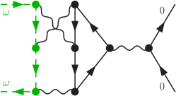
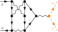
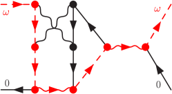
Figure 40: (Color online) A set of four diagrams for $\Gamma_{\uparrow\uparrow;\uparrow\uparrow}^{(4M)}$, contribution of which is given in Eq. (146).

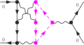
Figure 41: (Color online) Schematic picture for the total contribution $\widehat{\partial}_{i\omega}^{+}\Gamma_{\uparrow\uparrow;\uparrow\uparrow}^{(4M)}$ of the set shown in Fig. 40.

Total contribution of the diagrams shown in Fig. 40 can be rewritten in a total derivative form (see also Fig. 41):

$$\!\!\!\!\!\widehat{\partial}_{i\omega}^{+}\Gamma_{\uparrow\uparrow;\uparrow\uparrow}^{(4M)}(i\omega,0;0,i\omega)$$

$$=\,-U^{4}\int_{-\infty}^{\infty}\!\int_{-\infty}^{\infty}\!\int_{-\infty}^{\infty}\!\frac{d\varepsilon\,d\varepsilon_{1}\,d\varepsilon_{2}}{(2\pi)^{3}}\ \widehat{\partial}_{i\omega}^{+}\biggl{[}\,G_{\uparrow}(i\varepsilon_{1})\,G_{\uparrow}(i\varepsilon_{2})\,{\color[rgb]{0,0,1}G_{\downarrow}(i\varepsilon+i\varepsilon_{1}-i\varepsilon_{2}+i\omega)\,G_{\downarrow}(i\varepsilon-i\varepsilon_{2}+i\omega)\,G_{\downarrow}(i\varepsilon+i\omega)\,}G_{\downarrow}(i\varepsilon)\,$$

$$\qquad\qquad\qquad\qquad\qquad+{\color[rgb]{1,0,0}G_{\uparrow}(i\varepsilon_{1}+i\omega)\,G_{\uparrow}(i\varepsilon_{2}+i\omega)\,}G_{\downarrow}(i\varepsilon+i\varepsilon_{1}-i\varepsilon_{2})\,G_{\downarrow}(i\varepsilon-i\varepsilon_{2})\,G_{\downarrow}(i\varepsilon)\,{\color[rgb]{1,0,0}G_{\downarrow}(i\varepsilon+i\omega)\,}$$

$$\qquad\qquad\qquad\qquad\qquad-{\color[rgb]{0,0.5,0}G_{\uparrow}(i\varepsilon_{1}+i\omega)\,G_{\uparrow}(i\varepsilon_{2}+i\omega)\,}G_{\downarrow}(i\varepsilon+i\varepsilon_{1}-i\varepsilon_{2})\,G_{\downarrow}(i\varepsilon-i\varepsilon_{2})\,G_{\downarrow}(i\varepsilon)\,G_{\downarrow}(i\varepsilon)\,$$

$$\qquad\qquad\qquad\qquad\qquad-G_{\uparrow}(i\varepsilon_{1})\,G_{\uparrow}(i\varepsilon_{2})\,G_{\downarrow}(i\varepsilon+i\varepsilon_{1}-i\varepsilon_{2})\,G_{\downarrow}(i\varepsilon-i\varepsilon_{2})\,G_{\downarrow}(i\varepsilon)\,G_{\downarrow}(i\varepsilon)\,\,\biggr{]}$$

$$=\ -U^{4}\int_{-\infty}^{\infty}\!\int_{-\infty}^{\infty}\!\frac{d\varepsilon_{1}\,d\varepsilon_{2}}{(2\pi)^{2}}\ G_{\uparrow}(i\varepsilon_{1})\,G_{\uparrow}(i\varepsilon_{2})\int_{-\infty}^{\infty}\!\frac{d\varepsilon}{2\pi}\ \widehat{\partial}_{i\omega}^{+}\biggl{[}\,{\color[rgb]{0,0,1}G_{\downarrow}(i\varepsilon+i\varepsilon_{1}-i\varepsilon_{2}+i\omega)\,G_{\downarrow}(i\varepsilon-i\varepsilon_{2}+i\omega)\,G_{\downarrow}(i\varepsilon+i\omega)\,}G_{\downarrow}(i\varepsilon)\,$$

$$\qquad\qquad+G_{\downarrow}(i\varepsilon+i\varepsilon_{1}-i\varepsilon_{2})\,G_{\downarrow}(i\varepsilon-i\varepsilon_{2})\,G_{\downarrow}(i\varepsilon)\,{\color[rgb]{1,0,0}G_{\downarrow}(i\varepsilon+i\omega)\,}-2G_{\downarrow}(i\varepsilon+i\varepsilon_{1}-i\varepsilon_{2})\,G_{\downarrow}(i\varepsilon-i\varepsilon_{2})\,G_{\downarrow}(i\varepsilon)\,G_{\downarrow}(i\varepsilon)\,\,\,\biggr{]}$$

$$=-U^{4}\!\!\int_{-\infty}^{\infty}\!\!\int_{-\infty}^{\infty}\!\!\frac{d\varepsilon_{1}d\varepsilon_{2}}{(2\pi)^{2}}\,G_{\uparrow}(i\varepsilon_{1})\,G_{\uparrow}(i\varepsilon_{2})\ {\color[rgb]{1,0,1}\widehat{\partial}_{i\omega}^{+}\left[\int_{-\infty}^{\infty}\!\!\frac{d\varepsilon}{2\pi}\ G_{\downarrow}(i\varepsilon+i\varepsilon_{1}-i\varepsilon_{2}+i\omega)\,G_{\downarrow}(i\varepsilon-i\varepsilon_{2}+i\omega)\,\left\{G_{\downarrow}(i\varepsilon+i\omega)\right\}^{2}\,\right]}$$

$$=\ 0\;.$$ (146)

To obtain the second line, the derivative with respect to $\widehat{\partial}_{i\omega}^{+}$ is taken for $\omega$’s which are assigned for the $\uparrow$ spin propagators in the vertical direction. The remaining contribution arising from the two diagrams in the lower panel of Fig. 40 is extracted by applying the generalized chain rule for the product $G_{\downarrow}(i\varepsilon)G_{\downarrow}(i\varepsilon+i\omega)$.

 

 

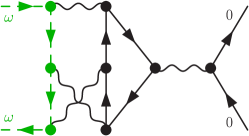
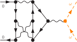
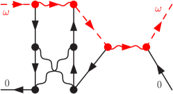
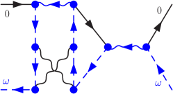
Figure 42: (Color online) A set of four diagrams for $\Gamma_{\uparrow\uparrow;\uparrow\uparrow}^{(4L^{\prime})}$. The contribution of which the same as that of $\Gamma_{\uparrow\uparrow;\uparrow\uparrow}^{(4L)}$ in Eq. (145).

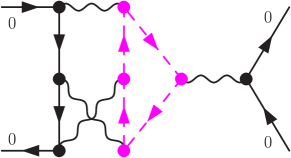
Figure 43: (Color online) Schematic picture for the total contribution $\widehat{\partial}_{i\omega}^{+}\Gamma_{\uparrow\uparrow;\uparrow\uparrow}^{(4L^{\prime})}$ of the diagrams shown in Fig. 42. Note that the contribution of this set $(4L^{\prime})$ is the same the contribution of $(4L)$.

Total contribution of the diagrams shown in Fig. 42 can be rewritten in a total derivative form as illustrated in Fig. 43. This set ($4L^{\prime}$) gives the same contribution as that of the set ($4L$) described in in Fig. 38, namely it also vanishes $\widehat{\partial}_{i\omega}^{+}\Gamma_{\uparrow\uparrow;\uparrow\uparrow}^{(4L^{\prime})}=0$. It can be confirmed, for instance, by interchanging the internal frequencies $\varepsilon_{1}$ and $\varepsilon_{2}$ in Eq. (145): then one get the corresponding expression for ($4L^{\prime}$) in our way of the frequency assignment.

 

 

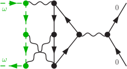
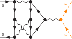
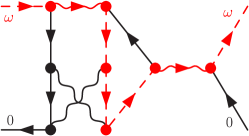
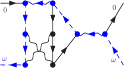
Figure 44: (Color online) A set of four diagrams for $\Gamma_{\uparrow\uparrow;\uparrow\uparrow}^{(4M^{\prime})}$ The contribution of which the same as that of $\Gamma_{\uparrow\uparrow;\uparrow\uparrow}^{(4M)}$ in Eq. (146).

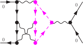
Figure 45: (Color online) Schematic picture for the total contribution $\widehat{\partial}_{i\omega}^{+}\Gamma_{\uparrow\uparrow;\uparrow\uparrow}^{(4M^{\prime})}$ of the set shown in Fig. 44. Note that the contribution of this set $(4M^{\prime})$ is the same the contribution of $(4M)$.

Total contribution of the diagrams shown in Fig. 44 can be rewritten in a total derivative form as illustrated in Fig. 45. This set ($4M^{\prime}$) gives the same contribution as that of the set ($4M$) described in in Fig. 40, namely it also vanishes $\widehat{\partial}_{i\omega}^{+}\Gamma_{\uparrow\uparrow;\uparrow\uparrow}^{(4M^{\prime})}=0$. It can be confirmed, for instance, by interchanging the internal frequencies $\varepsilon_{1}$ and $\varepsilon_{2}$ in Eq. (146): then one get the corresponding expression for ($4M^{\prime}$) in our way of the frequency assignment.