Some New Results on Charged Compact Boson Stars

Abstract

In this work we present some new results obtained in a study of the phase diagram of charged compact boson stars in a theory involving a complex scalar field with a conical potential coupled to a U(1) gauge field and gravity. We here obtain new bifurcation points in this model. We present a detailed discussion of the various regions of the phase diagram with respect to the bifurcation points. The theory is seen to contain rich physics in a particular domain of the phase diagram.

In this work we study the phase diagram of charged compact boson stars in a theory involving a complex scalar field with a conical potential coupled to a U(1) gauge field and gravity [1, 2]. A study of the phase diagram of the theory yields new bifurcation points (in addition to the first one obtained earlier, cf. Refs. [1, 2]), which implies rich physics in the phase diagram of the theory. In particular, we present a detailed discussion of the various regions in the phase diagram with respect to the bifurcation points.

Let us recall that the boson stars (introduced long ago [3, 4, 5]) represent localized self-gravitating solutions studied widely in the literature [6, 7, 8, 9, 10, 1, 2, 11, 12, 13, 17, 16, 14, 15].

In Refs. [16, 17], three of us have undertaken studies of boson stars and boson shells in a theory involving a massive complex scalar field coupled to a $U(1)$ gauge field $A_{\mu}$ and gravity in the presence of a cosmological constant $\Lambda$. Our present studies extend the work of Refs. [1, 2]), performed in a theory without a cosmological constant $\Lambda$ for a complex scalar field with only a conical potential, i.e., the scalar field is considered to be massless. Such a choice is possible for boson stars in a theory with a conical potential, since this potential yields compact boson star solutions with sharp boundaries, where the scalar field vanishes. This is in contrast to the case of non-compact boson stars, where the the mass of the scalar field is a basic ingredient for the asymptotic exponential fall-off of the solutions.

We construct the boson star solutions of this theory numerically. Our numerical method is based on the Newton-Raphson scheme with an adaptive stepsize Runge-Kutta method of order 4. We have calibrated our numerical techniques by reproducing the work of Refs. [1, 2] and [14, 15, 16, 17].

We consider the theory defined by the following action (with $V(|\Phi|):=\lambda|\Phi|$, where $\lambda$ is a constant parameter):

$$S = \int\left[\frac{R}{16\pi G}+\mathcal{L}_{M}\right]\sqrt{-g}\ d^{4}\,x\;,$$

$$\mathcal{L}_{M} = -\frac{1}{4}F^{\mu\nu}F_{\mu\nu}-\left(D_{\mu}\Phi\right)^{*}\left(D^{\mu}\Phi\right)-V(|\Phi|)\,,$$

$$D_{\mu}\Phi = (\partial_{\mu}\Phi+ieA_{\mu}\Phi)\ \ ,$$

$$\ \ F_{\mu\nu} = (\partial_{\mu}A_{\nu}-\partial_{\nu}A_{\mu}).$$ (1)

Here $R$ is the Ricci curvature scalar, $G$ is Newton’s gravitational constant. Also, $g=det(g_{\mu\nu})$, where $g_{\mu\nu}$ is the metric tensor, and the asterisk in the above equation denotes complex conjugation. Using the variational principle, the equations of motion are obtained as:

$$G_{\mu\nu} \equiv R_{\mu\nu}-\frac{1}{2}g_{\mu\nu}R=8\pi GT_{\mu\nu}\,,$$

$$\partial_{\mu}\left(\sqrt{-g}F^{\mu\nu}\right) = -ie\sqrt{-g}[\Phi^{*}(D^{\nu}\Phi)-\Phi(D^{\nu}\Phi)^{*}]\,,$$

$$D_{\mu}\left(\sqrt{-g}D^{\mu}\Phi\right) = \frac{\lambda}{2}\sqrt{-g}\,\frac{\Phi}{|\Phi|}\,,$$

$$\left[D_{\mu}\left(\sqrt{-g}D^{\mu}\Phi\right)\right]^{*} = \frac{\lambda}{2}\sqrt{-g}\,\frac{\Phi^{*}}{|\Phi|}.$$ (2)

The energy-momentum tensor $T_{\mu\nu}$ is given by

$$T_{\mu\nu} = \biggl{[}(F_{\mu\alpha}F_{\nu\beta}\ g^{\alpha\beta}-\frac{1}{4}g_{\mu\nu}F_{\alpha\beta}F^{\alpha\beta})$$

$$+(D_{\mu}\Phi)^{*}(D_{\nu}\Phi)+(D_{\mu}\Phi)(D_{\nu}\Phi)^{*}$$

$$-g_{\mu\nu}\left((D_{\alpha}\Phi)^{*}(D_{\beta}\Phi)\right)g^{\alpha\beta}-g_{\mu\nu}\lambda(|\Phi|)\biggr{]}.\ \ \$$

To construct spherically symmetric solutions we adopt the static spherically symmetric metric with Schwarzschild-like coordinates

$$ds^{2}=\biggl{[}-A^{2}Ndt^{2}+N^{-1}dr^{2}+r^{2}(d\theta^{2}+\sin^{2}\theta d\phi^{2})\biggr{]}.$$ (4)

This leads to the components of Einstein tensor ($G_{\mu\nu}$)

$$G_{t}^{t} = \biggl{[}\frac{-\left[r\left(1-N\right)\right]^{\prime}}{r^{2}}\biggr{]},$$

$$G_{r}^{r} = \biggl{[}\frac{2rA^{\prime}N-A\left[r\left(1-N\right)\right]^{\prime}}{A\ r^{2}}\biggr{]},$$

$$G_{\theta}^{\theta} = \biggl{[}\frac{2r\left[rA^{\prime}\ N\right]^{\prime}+\left[A\ r^{2}N^{\prime}\right]^{\prime}}{2A\ r^{2}}\biggr{]}\ \ =\ G_{\varphi}^{\varphi}.$$ (5)

Here the arguments of the functions $A(r)$ and $N(r)$ have been suppressed. For solutions with a vanishing magnetic field, the Ansätze for the matter fields have the form:

$$\Phi(x^{\mu})=\phi(r)e^{i\omega t}\ \ ,\ \ A_{\mu}(x^{\mu})dx^{\mu}=A_{t}(r)dt.$$ (6)

We introduce new constant parameters:

$$\beta=\frac{\lambda\,e}{\sqrt{2}}\ \ \ ,\ \ \ \alpha^{2}(:=a)=\frac{4\pi G\,\beta^{2/3}}{e^{2}}.$$ (7)

Here $a:=\alpha^{2}$ is dimensionless. We then redefine $\phi(r)$ and $A_{t}(r)$:

$$h(r)=\frac{(\sqrt{2}\;e\,\phi(r))}{\beta^{1/3}}\ \ \ ,\ \ \ b(r)=\frac{(\omega+eA_{t}(r))}{\beta^{1/3}}.$$ (8)

Introducing a dimensionless coordinate $\hat{r}$ defined by $\hat{r}:=\beta^{1/3}\,{r}$ (implying $\frac{d}{d{r}}=\beta^{1/3}\frac{d}{d\hat{r}}$), Eq. (8) reads:

$$h(\hat{r})=\frac{(\sqrt{2}\;e\,\phi(\hat{r}))}{\beta^{1/3}}\ \ \ ,\ \ \ b(\hat{r})=\frac{(\omega+eA_{t}(\hat{r}))}{\beta^{1/3}}.$$ (9)

The equations of motion in terms of $h(\hat{r})$ and $b(\hat{r})$ (where the primes denote differentiation with respect to $\hat{r}$, and ${\rm sign}(h)$ denotes the usual signature function) read:

$$\left[AN\hat{r}^{2}h^{\prime}\right]^{\prime} = \frac{\hat{r}^{2}}{AN}\left(A^{2}N{\rm sign}(h)-b^{2}h\right)\ ,$$ (10)

$$\left[\frac{\hat{r}^{2}b^{\prime}}{A}\right]^{\prime} = \frac{bh^{2}\hat{r}^{2}}{AN}.\$$ (11)

We thus obtain the set of equations:

$$N^{\prime} = \bigg{[}\frac{1-N}{\hat{r}}-\frac{\alpha^{2}\hat{r}}{A^{2}N}\left(A^{2}N^{2}h^{\prime 2}+Nb^{\prime 2}\right.$$ (12)

$$\hskip 72.26999pt\left.+2A^{2}Nh+b^{2}h^{2}\right)\bigg{]}\ ,$$

$$A^{\prime} = \bigg{[}\frac{\alpha^{2}\hat{r}}{AN^{2}}\left(A^{2}N^{2}h^{\prime 2}+b^{2}h^{2}\right)\bigg{]},$$ (13)

$$h^{\prime\prime} = \bigg{[}\frac{\alpha^{2}}{A^{2}N}\hat{r}h^{\prime}\left(2A^{2}h+b^{\prime 2}\right)-\frac{h^{\prime}\left(N+1\right)}{\hat{r}N}$$ (14)

$$\qquad+\frac{A^{2}N{\rm sign}(h)-b^{2}h}{A^{2}N^{2}}\bigg{]},$$

$$b^{\prime\prime} = \bigg{[}\frac{\alpha^{2}}{A^{2}N^{2}}\hat{r}b^{\prime}\left(A^{2}N^{2}h^{\prime 2}+b^{2}h^{2}\right)$$ (15)

$$\qquad-\frac{2b^{\prime}}{\hat{r}}+\frac{bh^{2}}{N}\bigg{]}.$$

For the metric function $A(\hat{r})$ we choose the boundary condition $A(\hat{r}_{o})=1$, where $\hat{r}_{o}$ is the outer radius of the star. For constructing globally regular ball-like boson star solutions, we choose:

$$N(0)=1\ ,\ \ b^{\prime}(0)=0\ ,$$

$$h^{\prime}(0)=0\ ,\ \ h(\hat{r}_{o})=0\ ,\ \ h^{\prime}(\hat{r}_{o})=0.$$ (16)

In the exterior region $\hat{r}>\hat{r}_{o}$ we match the Reissner-Nordström solution.

The theory has a conserved Noether current:

$$j^{\mu}=-i\,e\,\left[\Phi(D^{\mu}\Phi)^{*}-\Phi^{*}(D^{\mu}\Phi)\right]\ ,\ \ j^{\mu}_{\ ;\mu}=0\ .$$ (17)

The charge $Q$ of the boson star is given by

$$Q=-\frac{1}{4\pi}\int_{0}^{\hat{r}_{o}}j^{t}\sqrt{-g}\,dr\,d\theta\,d\phi\,,\ j^{t}=-\frac{h^{2}(\hat{r})b(\hat{r})}{A^{2}(\hat{r})N(\hat{r})}.$$

For all boson star solutions we obtain the mass $M$ (in the units employed):

$$M=\biggl{(}1-N(\hat{r}_{o})+\frac{\alpha^{2}Q^{2}}{\hat{r}_{o}^{2}}\biggr{)}\frac{\hat{r}_{o}}{2}.$$ (18)

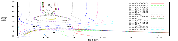
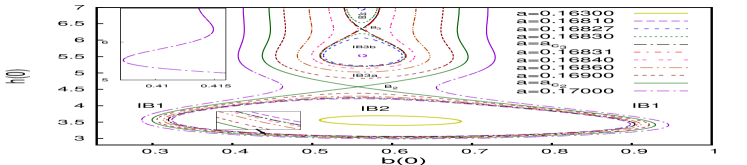
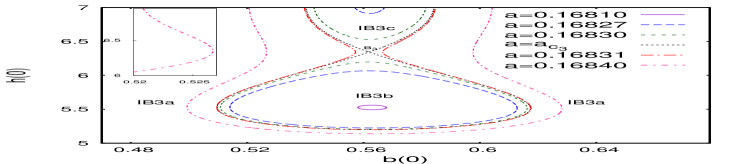
Figure 1: Fig. (a) depicts the phase diagram of the theory in terms of the vector field at the center of the star $b(0)$ and the scalar field at the center of the star $h(0)$ for different values of the parameter $a$ in the range $a=0$ to $a=0.225$. The points $B_{1},~{}B_{2}$ and $B_{3}$ represent three bifurcation points. The entire region depicted in the phase diagram in Fig. (a) is divided into four regions IA, IB and IIA, IIB in the vicinity of $B_{1}$. The region IB of the phase diagram shown in Fig. (a) is separately depicted in detail in Fig. (b). The region IB of the phase diagram is subdivided into three regions IB1, IB2 and IB3 in the vicinity of $B_{2}$. The region IB3 of the phase diagram shown in Fig. (b) is separately depicted in detail in Fig. (c). It is subdivided into three regions IB3a, IB3b and IB3c in the vicinity of $B_{3}$. The asterisks shown in Fig. (a), corresponding to $h(0)=0$, represent the transition points from the boson stars to boson shells. The insets in Figs. (b) and (c) represent parts of these phase diagrams with higher resolution.

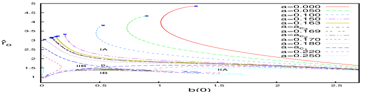
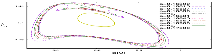
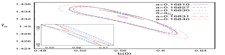
Figure 2: Fig. (a) shows the radius $\hat{r}_{o}$ of the boson star versus the vector field at the center of the star $b(0)$ for different values of $a$ in the range $a=0$ to $a=0.225$. The point $B_{1}$ corresponds to the first bifurcation point and the entire region depicted in Fig. (a) is divided into four regions IA, IB and IIA, IIB in the vicinity of $B_{1}$ (as in Fig. 1). The region IB shown in Fig. (a) is separately depicted in detail in Fig. (b) and similarly a part of the region shown in Fig. (b) is separately depicted in detail in Fig. (c). The asterisks shown in Fig. (a) represent the transition points from the boson stars to boson shells. The spiral behaviour of the solutions is visible in the regions IA and IIB. The inset in Fig. (c) represents a part of the region IIB with higher resolution.

We now study the numerical solutions of Eqs. (12)-(15) with the boundary conditions defined by $A(\hat{r}_{o})=1$ and Eq. (16), and determine their domain of existence for a sequence of specific values of the parameter $a$.

Let us recall here that the theory defined by the action (Eq. (Some New Results on Charged Compact Boson Stars)) originally has two parameters $e$ and $\lambda$ which are the two coupling constants of the theory. At a later stage we have introduced the new parameters $\beta$ and $a(:=\alpha^{2})$, and we have rescaled the radial coordinate and the matter functions. Then the parameter $\beta$ does not appear in the resulting set of equations (12)-(15). Thus the numerical solutions of these coupled differential equations can be studied by varying only one parameter, namely $a$.

We first consider the phase diagram of the theory based on the values of the fields at the origin of the boson star, the vector field, $b(0)$, and the scalar field, $h(0)$, obtained by studying a sequence of values of the parameter $a$. We observe very interesting phenomena near specific values of $a$, where the system is seen to have bifurcation points $B_{1}\,,\,B_{2}$ and $B_{3}$. These correspond to the following values of $a$: $a_{c_{1}}\simeq 0.198926,~{}a_{c_{2}}\simeq 0.169311$ and $a_{c_{3}}\simeq 0.168308$, respectively, and the possibility of further bifurcation points is not ruled out. Thus the theory is seen to possess rich physics in the domain $a=0.22$ to $a\simeq+0.16\,$.

For a clear discussion, we divide the phase diagram in the vicinity of $B_{1}$ into four regions denoted by IA, IB, IIA and IIB (as seen in Fig. 1). The asterisks seen in Fig. 1, coinciding with the axis $b(0)$ (which corresponds to $h(0)=0$), represent the transition points from the boson stars to boson shells [1, 2].

The regions IA, IIA and IIB do not have any further bifurcation points. However, the region IB is seen to contain rich physics as evidenced by the occurrence of more bifurcation points in this region. For better detail, the region IB is magnified in Fig. 1. The region IB is then further divided into the regions IB1, IB2 and IB3 in the vicinity of $B_{2}$, as seen in Fig. 1.

The region IB3 finally is seen to have the further bifurcation point $B_{3}$. In the vicinity of $B_{3}$ we therefore further subdivide the phase diagram into the regions IB3a, IB3b and IB3c, as seen in Fig. 1. The region IB3b is seen to have closed loops and the behaviour of the phase diagram in this region is akin to the one of the region IB2. Also, the insets shown in Figs. 1 and 1 represent parts of the phase diagram with higher resolution.

The figures demonstrate, that as we change the value of $a$ from $a=0.225$ to $a=0$, we observe a lot of new rich physics. While going from $a=0.225$ to the critical value $a=a_{c_{1}}$, we observe that the solutions exist in two separate domains, IIA and IIB (as seen in Fig. 1). However, as we decrease $a$ below $a=a_{c_{1}}$, the solutions of the theory are seen to exist in the regions IA and IB (instead of the regions IIA and IIB). For the sake of completeness it is important to emphasize here, that the physics in the domain corresponding to the values of $a$ larger than $a=0.225$ conceptually remains the same as described by the value $a=0.225\,$.

As we decrease the value of $a$ from the first critical value $a=a_{c_{1}}$ to the next critical value $a=a_{c_{2}}$, we notice that the region IA in the phase diagram shows a continuous deformation of the curves, and the region IB is seen to have its own rich physics as explained in the foregoing.

As we decrease $a$ below $a_{c_{2}}$, we observe that in the region IA there is again a continuous deformation of the curves all the way down to $a=0$. However in the region IB, we encounter another bifurcation point, which divides the region IB into IB1, IB2 and IB3. We observe that in the region IB1 there is a continuous deformation of the curves, and the region IB2 contains closed loops of the curves. The region IB3 is subdivided into the regions IB3a, IB3b and IB3c. The region IB3a would have a continuous deformation of the curves, and the region IB3b is seen to contain closed loops.

It is tempting to conjecture, that there is a whole sequence of further bifurcation points, leading to a self-similar pattern of the new subregions involved. The numerical calculations, however, become more and more challenging, as one proceeds from the first to the higher bifurcations, since an increasing numerical accuracy is necessary to map out the domain of existence. Note, that the value of $a$ had to be specified to 6 decimal digits for B2 and B3, already. Thus it is the global accuracy of the scheme, which presents a limiting factor. Within this accuracy, the Newton-Raphson method will provide a new solution, when an adequate starting solution has been specified, though.

A plot of the radius $\hat{r}_{o}$ of the solutions versus the vector field at the center of the star $b(0)$ is depicted in Fig. 2. As before, the point $B_{1}$ corresponds to the first bifurcation point, and the four regions IA, IB and IIA, IIB in the vicinity of the bifurcation point are indicated. Again, the region IB shown in Fig. 2 is enlarged and shown in Fig. 2, with the region IB3 being enlarged further and depicted in Fig. 2. The asterisks shown in Fig. 2 again represent the transition points from the boson stars to boson shells. The oscillating behaviour seen in Figs. 1 to 1 in the regions IIA and IB translates in the Figs. 2 to 2 into a spiral behavior. The inset in Fig. 2 represents a part of the region IB with higher resolution.

Let us now turn to the global properties of the solutions, their mass $M$ and their charge $Q$. The mass $M$ versus the radius $\hat{r}_{o}$ is shown in Fig. 3, while 3 again magnifies the region of the bifurcations. The charge $Q$ has a very similar dependence as the mass. This is illustrated in Fig. 3 for the bifurcation region.

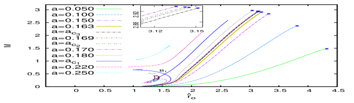
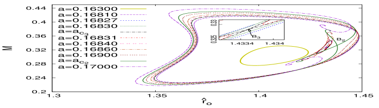
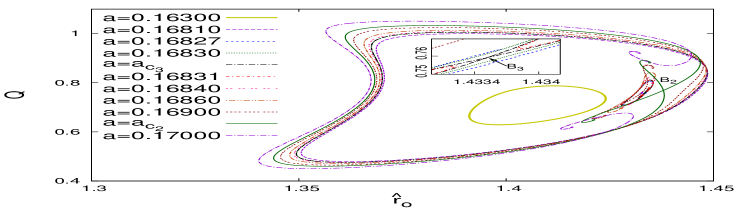
Figure 3: Fig. (a) depicts the mass $M$ versus the radius of the star $\hat{r}_{o}$ for the same sequence of values of the parameter $a$. As before, the asterisks represent the transition points from the boson stars to boson shells, and the insets magnify parts of the diagram. Fig. (b) zooms into the region of the bifurcations, with the inset giving a magnified view of the bifurcation B3. Fig. (c) is the analog of Fig. (b) for the charge $Q$.

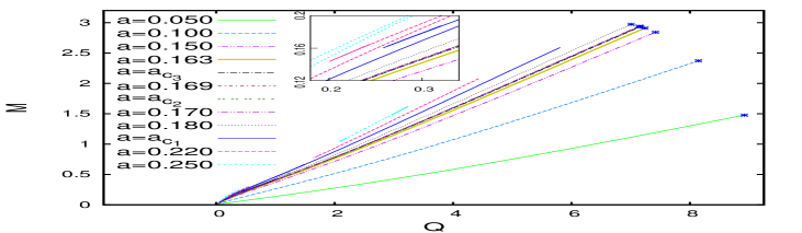
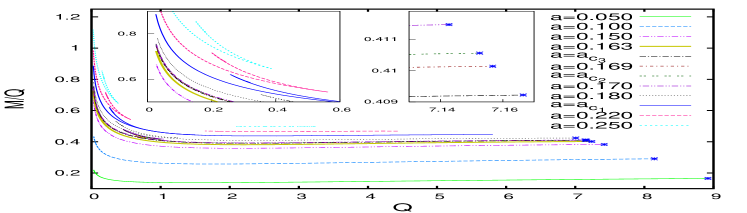
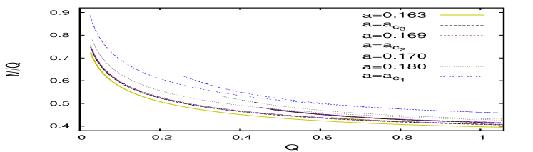
Figure 4: Fig. (a) depicts the mass $M$ versus the charge $Q$ for the same set of solutions. As before, the asterisks represent the transition points from the boson stars to boson shells, and the inset magnifies a part of the diagram. Fig. (b) depicts the mass per unit charge $M/Q$ versus the charge $Q$. Again the insets magnify parts of the diagram. Fig. (c) zooms further into the region of the bifurcations.

To understand the stability of the boson stars, one can consider the mass $M$ versus the charge $Q$, as shown in Fig. 4, or the mass per unit charge $M/Q$ versus the charge, as shown in Figs. 4 and 4. Let us first consider Fig. 4. Here the curves $M$ versus $Q$, corresponding to the region IA and the smaller values of $a$, all increase monotonically from $M=Q=0$ to the respective transition points with boson shells, marked by the crosses. The solutions on these curves can be considered as the fundamental solutions for their respective value of $a$. Thus they should be stable. In fact, all curves in region IA should be stable, representing the solutions with the lowest mass for a given charge (and parameter $a$). However, above a certain value of $a$, these curves no longer reach a boson shell, but instead their upper endpoint represents a solution, where a throat is formed. The exterior space-time $r>r_{0}$ then corresponds to the exterior of an extremal RN space-time. This happens whenever the value $b(0)=0$ is encountered, as discussed in detail previously [1, 2].

For the curves shown in region IIB both endpoints correspond to solutions with throats, since at both endpoints $b(0)=0$ is encountered. Since these solutions also represent the lowest mass solutions for a given charge, they should be stable as well. In the region IIA, however, the solutions exhibit the typical oscillating/spiral behavior known for non-compact boson stars. In a mass versus charge diagram, this translates into the presence of a sequence of spikes, as seen in the insets of Figs. 4 and 4. Here the solutions should be stable only on their fundamental branch, reaching up to a maximal value of the mass and the charge, where a first spike is encountered. With every following spike a new unstable mode is expected to arise, as we conclude by analogy with the properties of non-compact boson stars.

In this work our focus has been on the bifurcations. Let us therefore now inspect the region of the bifurcations IB, starting with the limiting curves. For the value $a_{c_{1}}$ the two branches of solutions, limiting the region IA, possess lower masses than the the two branches of solutions, limiting the region IB, and should therefore be more stable. The two branches of solutions, limiting the region IB, might be classically stable as well, until the first extrema of mass and charge are encountered. Quantum mechanically, however, they would be unstable, since tunnelling might occur. Beyond these extrema, unstable modes should be present, and thus the solutions should also be classically unstable.

These arguments can be extended to all the solutions in region IB. From a quantum point of view they should be unstable, since for all of them there exist solutions in region IA, which have lower masses but possess the same values of the charge. Classically, however, the lowest mass solutions for a given $a$ within the region IB might be stable, while the higher mass solutions should clearly possess unstable modes and be classically unstable. Fig. 4 zooms into the bifurcation region of the $M/Q$ versus $Q$ diagram, to illustrate that the solutions in the bifurcation region indeed correspond to higher mass solutions.

In conclusion, we have studied in this work a theory of a complex scalar field with a conical potential, coupled to a U(1) gauge field and gravity [1, 2]. We have constructed the boson star solutions of this theory numerically and investigated their domain of existence, their phase diagram, and their physical properties.

We have shown that the theory has rich physics in the domain $a=0.22$ to $a\simeq 0.16$, where we have identified three bifurcation points $B_{1},~{}B_{2}$ and $B_{3}$ of possibly a whole sequence of further bifurcations. We have investigated the physical properties of the solutions, including their mass, charge and radius. By considering the mass versus the charge (or the mass per unit charge versus the charge) we have given arguments concerning the stability of the solutions.

For all values of $a$ studied, there is a fundamental branch of compact boson star solutions, which should be stable, since they represent the solutions with the lowest mass for a given value of the charge, and thus represent the ground state. In the region of the bifurcations additional branches of solutions are present, which possess higher masses for a given charge. Thus these solutions correspond to excited states of the system. The lowest of these might be classically stable, as well, and only quantum mechanically unstable. To definitely answer this question, a mode stability analysis should be performed, which is, however, beyond the scope of this paper, representing a topic of separate full-fledged investigations.

Finally, we would like to mention that detailed investigations of this theory in the presence of the cosmological constant $\Lambda$ with 3D plots of the phase diagrams involving the various physical quantities of the theory are currently under our investigation and would be reported later separately.

We would like to thank James Vary for very useful discussions. This work was supported in part by the US Department of Energy under Grant No. DE-FG02-87ER40371, by the US National Science Foundation under Grant No. PHY-0904782, by the DFG Research Training Group 1620 Models of Gravity as well as by FP7, Marie Curie Actions, People IRSES-606096. SK would like to thank the CSIR, New Delhi, for the award of a Research Associateship.

References

- [1] B. Kleihaus, J. Kunz, C. Lämmerzahl and M. List, “Charged Boson Stars and Black Holes”, Phys. Lett. B 675, (2009) 102, [arXiv:0902.4799 [gr-qc]].
- [2] B. Kleihaus, J. Kunz, C. Lämmerzahl and M. List, “Boson Shells Harbouring Charged Black Holes”, Phys. Rev. D82, (2010) 104050, [arXiv:1007.1630 [gr-qc]].
- [3] D. A. Feinblum, W. A. McKinley, “Stable states of a scalar particle in its own gravitational field”, Phys. Rev. 168, 1445 (1968).
- [4] D. J. Kaup, “Klein-Gordon Geon,” Phys. Rev. 172, 1331 (1968).
- [5] R. Ruffini, S. Bonazzola, “Systems of selfgravitating particles in general relativity and the concept of an equation of state,” Phys. Rev. 187, 1767 (1969).
- [6] P. Jetzer, “Boson Stars”, Phys. Rept. 220 (1992) 163.
- [7] T. D. Lee and Y. Pang, “Nontopological solitons”, Phys. Rept. 221, (1992) 251.
- [8] E. W. Mielke and F. E. Schunck, “Boson stars: Alternatives to primordial black holes?,” Nucl. Phys. B 564, 185 (2000). [arXiv:gr-qc/0001061].
- [9] S. L. Liebling and C. Palenzuela, “Dynamical Boson Stars,” Living Rev. Rel. 15, 6 (2012) [arXiv:1202.5809 [gr-qc]].
- [10] R. Friedberg, T. D. Lee and A. Sirlin, “A Class Of Scalar-Field Soliton Solutions In Three Space Dimensions,” Phys. Rev. D 13, 2739 (1976).
- [11] B. Hartmann, B. Kleihaus, J. Kunz, I. Schaffer, Compact boson stars, Phys. Lett. B 714, (2012) 120, [arXiv:1205.0899 [gr-qc]].
- [12] B. Hartmann and J. Riedel, “Glueball condensates as holographic duals of supersymmetric Q-balls and boson stars,” Phys. Rev. D 86, 104008 (2012)
- [13] B. Hartmann, B. Kleihaus, J. Kunz and I. Schaffer, “Compact (A)dS Boson Stars and Shells,” Phys. Rev. D 88, 124033 (2013), [arXiv:1310.3632 [gr-qc]].
- [14] S. Kumar, U. Kulshreshtha and D. Shankar Kulshreshtha, “Boson stars in a theory of complex scalar fields coupled to the U(1) gauge field and gravity,” Class. Quant. Grav. 31, 167001 (2014).
- [15] S. Kumar, U. Kulshreshtha and D. S. Kulshreshtha, “Boson stars in a theory of complex scalar field coupled to gravity,” Gen. Rel. Grav. 47, 76 (2015).
- [16] S. Kumar, U. Kulshreshtha and D. S. Kulshreshtha, “New Results on Charged Compact Boson Stars,” Phys. Rev. D 93, 101501 (2016) [arXiv:1605.02925 [hep-th]].
- [17] S. Kumar, U. Kulshreshtha and D. S. Kulshreshtha, “Charged compact boson stars and shells in the presence of a cosmological constant,” Phys. Rev. D 94, 125023 (2016).