The quasi-optimality criterion in the linear functional strategy

Abstract

The linear functional strategy for the regularization of inverse problems is considered. For selecting the regularization parameter therein, we propose the heuristic quasi-optimality principle and some modifications including the smoothness of the linear functionals. We prove convergence rates for the linear functional strategy with these heuristic rules taking into account the smoothness of the solution and the functionals and imposing a structural condition on the noise. Furthermore, we study these noise conditions in both a deterministic and stochastic setup and verify that for mildly-ill-posed problems and Gaussian noise, these conditions are satisfied almost surely, where on the contrary, in the severely-ill-posed case and in a similar setup, the corresponding noise condition fails to hold. Moreover, we propose an aggregation method for adaptively optimizing the parameter choice rule by making use of improved rates for linear functionals. Numerical results indicate that this method yields better results than the standard heuristic rule.

Keywords: regularization, linear functional strategy, heuristic parameter choice rules, quasi-optimality rule, aggregation

AMS subject classifications: 65J20, 47A52, 65F22

1 Introduction

The estimation of linear bounded functionals of an unknown element $x$ from an indirect noisy observation $y^{\delta}$ given as

$$y^{\delta}=Tx+\delta\xi$$ (1.1)

is one of the classical problems in regularization theory [2]. Here, we assume that $T$ is a linear, injective, not necessarily boundedly invertible operator from a solution Hilbert space $X$ into an observation Hilbert space $Y$, $\xi$ is an additive noise process, and $\delta$ is its intensity, or noise level, such that for $y=Tx$, it holds $\left\|y-y^{\delta}\right\|\leq\delta$, $\delta\in(0,1)$. We use the same symbols $\left\langle\cdot,\cdot\right\rangle$, $\left\|\cdot\right\|$ for the inner products and the corresponding norms in both $X$ and $Y$.

It is known that the problem of estimating the value $f(x)=\langle f,x\rangle$ of a linear bounded functional $f\in X$ from (1.1) is less ill-posed than the problem of estimating $x$, in the sense that the value $f(x)$ allows for a more accurate reconstruction than the element $x$ in the $X$-norm [10, 3, 17]. A regularization of the first-named problem is usually performed by the so-called linear functional strategy [1] that is also closely related to the mollifier methods [16]. In case of a known noise intensity $\delta$, the choice of the regularization parameters in the linear functional strategy has been extensively studied (see, e.g., [11, 18, 17] and references therein).

At the same time, in some applications, such as satellite gravity gradiometry, one cannot expect to have good knowledge of the noise model in general and of the noise intensity $\delta$ in particular (see, e.g., discussions in [14, 5]). As a remedy for this, regularization theory has an arsenal of so-called heuristic parameter choice strategies that do not require knowledge of the noise intensity and therefore can be used in the above mentioned applications. The quasi-optimality criterion [21] is one of the simplest and the oldest but still quite efficient instance among such strategies.

Of course, in the worst case scenario, where the noise $\xi$ in (1.1) is assumed to be chosen by some antagonistic opponent only subject to the constraint $\left\|\xi\right\|\leq 1$, the quasi-optimality criterion, as well as any other heuristic parameter choice strategy, cannot guarantee convergence of the corresponding regularized approximants because of the so-called Bakushinskii veto [4]. On the other hand, it has been shown [6, 7] that for the quasi-optimality criterion, the Bakushinskii veto can be avoided if the regularization performance is measured on average over realizations of $\xi$.

At the same time, another way to overcome the Bakushinskii veto has been proposed in [13, 19], where convergence of the regularized approximants to $x$ in the solution space norm and its rates have been established under a qualitative restriction on the noise $\xi$ (a noise condition of Muckenhoupt type). Our intention in this paper is to extend this restricted noise approach in [13, 19] to the context of the linear functional strategy. We also show that for a wide class of moderately ill-posed problems (1.1) and for random noise $\xi$ with bounded moments, the above mentioned Muckenhoupt-type condition is satisfied almost surely.

The case of severely ill-posed problems is considered as well. Note that in this case, the theoretical bounds on the convergence rates of the regularized approximants selected by the quasi-optimality criterion in the solution space norm are worse than those for the noise level-dependent parameter choice strategies. At the same time, as follows from our results, in the linear functional strategy, the above-mentioned convergence rate gap can be essentially reduced. This hints at an opportunity to use the linear functional strategy equipped with the quasi-optimality criterion for aggregating the constructed regularized approximants in a way described in [9]. Then from [9], it follows that such aggregation by the linear functional strategy can improve the accuracy compared to the aggregated regularized approximations, and this can be seen as a way to use the quasi-optimality criterion for mildly and severely ill-posed problems.

Note that a practical implementation of the quasi-optimality criterion depends on the so-called differential quadrature [8]

$$\left.\frac{\partial x_{\alpha}^{\delta}}{\partial\alpha}\right|_{\alpha=\alpha_{i}}\approx\sum\limits_{j}a_{ij}x_{\alpha_{j}}^{\delta}$$ (1.2)

that is used to approximate the partial derivative $\frac{\partial x_{\alpha}^{\delta}}{\partial\alpha}$ of the regularized solution $x_{\alpha}^{\delta}$ of (1.1), which is based on a current value of the regularization parameter $\alpha=\alpha_{i}$. Starting from the original paper [21], one usually uses a simple backward difference formula, where $a_{ij}=0$ for $j\neq i,i-1$, and $a_{i,i}=-a_{i,i-1}=\left(\alpha_{i}-\alpha_{i-1}\right)^{-1}$.

On the other hand, as it is mentioned in [8], there are many ways of determining the coefficients $a_{ij}$ in (1.2). For example, in the backward difference formula, one can introduce correction factors such that

$$a_{i,i}=c_{i}\left(\alpha_{i}-\alpha_{i-1}\right)^{-1},\quad a_{i,i-1}=-c_{i-1}\left(\alpha_{i}-\alpha_{i-1}\right)^{-1},$$

where $c_{\ell}$, $\ell=i,i-1$, approximates the values $c_{\ell}^{*}$ minimizing the error $\left\|x-c_{\ell}^{*}x_{\alpha_{\ell}}^{\delta}\right\|=\min\limits_{c}\left\|x-cx_{\alpha_{\ell}}^{\delta}\right\|$. It is clear that $c_{\ell}^{*}=\left\langle x,x_{\alpha_{\ell}}^{\delta}\right\rangle/\left\|x_{\alpha_{\ell}}^{\delta}\right\|^{2}$, and $\left\langle x,x_{\alpha_{\ell}}^{\delta}\right\rangle$ is the value of the linear bounded functional $x_{\alpha_{\ell}}^{\delta}\in X$ at the unknown solution that can be approximated by $\left\langle x_{\alpha_{j}}^{\delta},x_{\alpha_{\ell}}^{\delta}\right\rangle$, where $\alpha_{j}$ is chosen by the quasi-optimality criterion.

The use of the backward difference formula corrected as above can be seen as an iterated quasi-optimality rule. We will demonstrate in Section 5 that such a combination of the linear functional strategy—by an aggregation approach— and the quasi-optimality criterion can also improve the regularization performance as compared to the standard quasi-optimality.

The paper is organized as follows. In the next section, we present the problem setup and formulate main results. The proofs are given in Section 3. In Section 4, we describe random processes and investigate whether they almost surely meet the Muckenhoupt-type conditions. In Section 5, we discuss a combination of the aggregation by means of the linear functional strategy with the quasi-optimality criterion and present numerical experiments.

2 The main convergence rates results

In this section, we formulate the main results. Let us introduce some standard notation. Let $X,Y$ be Hilbert spaces, $T:X\to Y$ be a continuous linear operator such that $Ker(T)=\{0\}$, $Ker(T^{*})=\{0\}.$ Here, the assumptions of injectivity of $T$ and $T^{*}$ are only imposed for simplicity; the main results hold with modifications in the general case as well. We denote by $E_{\lambda}$ and $F_{\lambda}$ the spectral families for the operators $T^{*}T$ and $TT^{*}$, respectively. The notion $R(T)$ stands for the range and $Ker(T)$ for the nullspace of the operator $T$. For $f,g$ being functions or sequences, the notation $f\asymp g$ indicates that some constants $c_{1},c_{2}$ exist such that $c_{1}f\leq g\leq c_{2}f$ for all arguments or sequence indices, where the constants in particular do not depend on $\delta$.

Consider an ill-posed problem in the form $Tx=y$. Suppose that we observe $y^{\delta}\in Y$ such that $\|y^{\delta}-y\|\leq\delta.$ We introduce regularized solutions obtained by a general spectral filter function $g_{\alpha}$:

$$x_{\alpha}=g_{\alpha}(T^{*}T)T^{*}y,\ \ x_{\alpha}^{\delta}=g_{\alpha}(T^{*}T)T^{*}y^{\delta}.$$

Moreover, let $f\in X^{*}=X$ be a linear functional.

One aim of this paper is to obtain upper bounds for the error of linear functionals of the solutions, i.e., for the quantity $\langle f,x_{\alpha(y^{\delta})}^{\delta}-x\rangle$, where a parameter $\alpha(y^{\delta})$ is selected in a special way and depends only on the observation $y^{\delta}.$ To state a smoothness/source condition for $x$ and/or $f$, we use $\varphi$ and $\varkappa$, which are continuous, non-negative, increasing real functions defined for positive real values (so-called index functions). Below we impose some standard assumptions on $\varphi,\varkappa,g_{\alpha}$.

Convergence rates estimates for the error $x_{\alpha}-x$ using some smoothness conditions on $x$ are nowadays a classical topic. For instance, if $\delta$ is known, see, for example, [17], then under some natural conditions the best accuracy that can be guaranteed under the smoothness condition $x\in R(\varphi(T^{*}T))$ is of the order $\varphi(\theta^{-1}(\delta))$, where $\theta(t)=\varphi(t)\sqrt{t}$ and $\theta^{-1}$ is its inverse function. For linear functionals, the situation can be improved: Assume that $x\in R(\varphi(T^{*}T)),$ and $f\in R(\varkappa(T^{*}T))$, where $\varphi,\varkappa$ are index functions, then the best accuracy for the linear functionals $\langle f,x_{\alpha(y^{\delta})}^{\delta}-x\rangle$ is of the order $(\varkappa\varphi)(\theta^{-1}(\delta))$.

If the noise intensity is known, then the best order in accuracy can usually be achieved by standard means of selecting $\alpha$. However, if $\delta$ is not known, the choice of the optimal $\alpha$ is a serious problem. For $\alpha(y^{\delta})$ selected according to the quasi-optimality principle, some upper bounds for $\|x_{\alpha(y^{\delta})}^{\delta}-x\|$ were obtained in [13, 19]. There it is proved that if $\varphi(t)=t^{\mu}$ and if the qualification $\mu_{0}$ of the regularization $g_{\alpha}$ is such that $\mu_{0}\geq\mu$, then

$$\|x_{\alpha(y^{\delta})}^{\delta}-x\|=O(\delta^{\frac{2\mu}{2\mu+1}\frac{\mu}{\mu_{0}}}),\ \delta\to 0.$$

The main assumption on the noise was the following condition of Muckenhoupt type (noise condition):

$$\exists C>0\ \forall\delta>0\ \forall\alpha>0\qquad\alpha^{2}\int_{\alpha}^{\infty}\lambda^{-1}d\|F_{\lambda}(y^{\delta}-y)\|^{2}\leq C\int_{0}^{\alpha}\lambda d\|F_{\lambda}(y^{\delta}-y)\|^{2}.$$ (2.1)

We give some sufficient conditions that ensure (2.1) in Section 4. In this paper we consider (2.1) and its generalization for the linear functional strategy. We discuss these conditions in the deterministic and random case; in particular we verify that for mildly ill-posed problems and Gaussian noise, it is satisfied almost surely. Moreover, we provide upper bounds for $\langle f,x_{\alpha(y^{\delta})}^{\delta}-x\rangle$, where $\alpha(y^{\delta})$ is selected by the quasi-optimality principle as in [13, 19], and we also obtain some generalization of the upper bounds there. Furthermore, we prove improved bounds $\langle f,x_{\alpha_{\varkappa}(y^{\delta})}^{\delta}-x\rangle$, when $\alpha_{\varkappa}(y^{\delta})$ is selected heuristically but using information about $y^{\delta}$ and also $\varkappa$.

For later use we introduce the quasi-optimality functional and a variant suited for functionals:

$$\psi^{2}(\alpha,y^{\delta}) =\int_{0}^{\infty}(1-\lambda g_{\alpha}(\lambda))^{2}\lambda g_{\alpha}^{2}(\lambda)d\|F_{\lambda}y^{\delta}\|^{2}=\|(I-T^{*}Tg_{\alpha}(T^{*}T))x_{\alpha}^{\delta}\|^{2},$$

$$\psi_{\varkappa}^{2}(\alpha,y^{\delta}) =\int_{0}^{\infty}\varkappa^{2}(\lambda)(1-\lambda g_{\alpha}(\lambda))^{2}\lambda g_{\alpha}^{2}(\lambda)d\|F_{\lambda}y^{\delta}\|^{2}$$

$$=\|\varkappa(T^{*}T)(I-T^{*}Tg_{\alpha}(T^{*}T))x_{\alpha}^{\delta}\|^{2}.$$

We introduce the following minimization-based heuristic parameter choice rules; the first one is the classical quasi-optimality rule as in [13, 19] while the second one is our modification:

$$\alpha(y^{\delta})=\textrm{argmin}_{\alpha}\psi(\alpha,y^{\delta}),\qquad\alpha_{\varkappa}(y^{\delta})=\textrm{argmin}_{\alpha}\psi_{\varkappa}(\alpha,y^{\delta}).$$ (2.2)

It is clear that $\alpha(y^{\delta})$ can be computed without knowledge of $\delta$, which is the defining feature of heuristic parameter choice rules. The novel modified rule $\alpha_{\varkappa}(y^{\delta})$ additionally needs knowledge of the functional smoothness (via $\varkappa)$). It will be shown that this additional information leads to improvements in the error bounds.

At first, we state some standard assumptions:

Assumption 1.

1. For all $\alpha>0$ we have

   $$0\leq\lambda g_{\alpha}(\lambda)\leq 1,\lambda>0,\qquad\sup_{\lambda>0}\sqrt{\lambda}g_{\alpha}(\lambda)\leq\frac{c_{1}}{\sqrt{\alpha}}.$$ (2.3)

2. For all $\alpha>0$ and $\lambda\in(0,\alpha)$

   $$(1-\lambda g_{\alpha}(\lambda))\geq c_{2},\qquad\frac{c_{3}}{\alpha}\leq g_{\alpha}(\lambda)\leq\frac{c_{4}}{\alpha}.$$ (2.4)

3. For any $\lambda>0$,

   $$k(\lambda):=\inf_{\alpha\in(0,\|T\|]}\frac{(1-\lambda g_{\alpha}(\lambda))g_{\alpha}(\lambda)}{\alpha}>0.$$ (2.5)

4. The qualification of $g_{\alpha}$ covers $\varphi$ and $\varphi\varkappa$, i.e., for all $\alpha>0$

   $$\sup_{\lambda>0}|\varphi(\lambda)(1-\lambda g_{\alpha}(\lambda))|\leq c_{5}\varphi(\alpha),$$ (2.6)

   $$\sup_{\lambda>0}|\varkappa(\lambda)\varphi(\lambda)(1-\lambda g_{\alpha}(\lambda))|\leq c_{6}\varkappa(\alpha)\varphi(\alpha).$$ (2.7)

5. The function $\varkappa$ is covered by the qualification $1/2$, i.e., for all $\alpha>0$

   $$\sup_{\lambda>\alpha}\varkappa(\lambda)/\sqrt{\lambda}\leq c_{7}\varkappa(\alpha)/\sqrt{\alpha}.$$ (2.8)

6. The function $\varkappa,\varphi$ are regularly varying: For all $c_{8}>0$ there exists $c_{9}>0$ and $\delta_{0}>0$ such that

   $$\varphi(c_{8}\delta)\leq c_{9}\varphi(\delta)\quad\mbox{ and }\quad\varkappa(c_{8}\delta)\leq c_{9}\varkappa(\delta)\qquad\forall\delta\in(0,\delta_{0}).$$ (2.9)

We note that in several places, condition (2.5) could be replaced by one with a more general qualification, i.e., that there exists $\mu_{0}>0$ such that for any $\lambda>0$

$$k(\lambda):=\inf_{\alpha\in(0,\|T\|]}\frac{(1-\lambda g_{\alpha}(\lambda))g_{\alpha}(\lambda)}{\alpha^{\mu_{0}}}>0.$$ (2.10)

Additionally to the structural conditions on the filter and index functions, we impose the following generalization of the noise condition (2.1):

$$\begin{split}&\exists\delta_{0}>0:\forall\delta\in(0,\delta_{0})\forall\alpha>0:\\ &\alpha^{2}\int_{\alpha}^{\infty}\lambda^{-1}\varkappa^{2}(\lambda)d\|F_{\lambda}(y^{\delta}-y)\|^{2}\leq c_{10}\int_{0}^{\alpha}\lambda\varkappa^{2}(\lambda)d\|F_{\lambda}(y^{\delta}-y)\|^{2}.\end{split}$$ (2.11)

We state the main convergence result of the paper. In the sequel we denote by $\vee$ the maximum.

Theorem 1.

Suppose that $y\neq 0,x\in R(\varphi(T^{*}T)),f\in R(\varkappa(T^{*}T)),$ where $\varphi,\varkappa$ are continuous, non-negative, increasing functions, the function $(0,\infty)^{2}\ni(\lambda,\alpha)\to g_{\alpha}(\lambda)$ is continuous, and there are constants $c_{1},\ldots,c_{9}>0$ such that Assumptions 1 hold. Moreover, let the noise condition (2.11) hold.

Then, as $\delta\to 0$,

$$|x_{\alpha(y^{\delta})}^{\delta}-x| =O\left(\varphi(\varphi(\theta^{-1}(\delta))\vee\varphi(\theta^{-1}(\delta))\right),$$ (2.12)

$$\begin{split}|\langle f,x_{\alpha(y^{\delta})}^{\delta}-x\rangle|&=O\left(\varkappa(\varphi(\theta^{-1}(\delta)))\varphi(\varphi(\theta^{-1}(\delta))\vee\varphi(\theta^{-1}(\delta))\right)\\ &=O\left((\varkappa\varphi)\circ(\varphi(\theta^{-1}(\delta)))\vee\varphi(\theta^{-1}(\delta))\right);\end{split}$$ (2.13)

$$|\langle f,x_{\alpha_{\varkappa}(y^{\delta})}^{\delta}-x\rangle| =O\left((\varkappa\varphi)\circ(\varkappa\varphi)(\theta^{-1}(\delta))\vee(\varkappa\varphi)(\theta^{-1}(\delta))\right).$$ (2.14)

Observe, that the bound (2.14) for the modified rule $\alpha_{\varkappa}(y^{\delta})$ is improved compared to (2.13).

Remark 1.

If we replace (2.5) by the more general one, (2.10), then the convergence rates in this theorem read as

$$|x_{\alpha(y^{\delta})}^{\delta}-x| =O\left(\varphi(\varphi^{1/\mu_{0}}(\theta^{-1}(\delta))\vee\varphi(\theta^{-1}(\delta))\right),$$ (2.15)

$$\begin{split}|\langle f,x_{\alpha(y^{\delta})}^{\delta}-x\rangle|&=O\left(\varkappa(\varphi^{1/\mu_{0}}(\theta^{-1}(\delta)))\varphi(\varphi(\theta^{-1}(\delta))\vee\varphi(\theta^{-1}(\delta))\right)\\ &=O\left((\varkappa\varphi)\circ(\varphi^{1/\mu_{0}}(\theta^{-1}(\delta)))\vee\varphi(\theta^{-1}(\delta))\right),\end{split}$$ (2.16)

$$|\langle f,x_{\alpha_{\varkappa}(y^{\delta})}^{\delta}-x\rangle| =O\left((\varkappa\varphi)\circ(\varkappa\varphi)^{1/\mu_{0}}(\theta^{-1}(\delta))\vee(\varkappa\varphi)(\theta^{-1}(\delta))\right).$$ (2.17)

Remark 2.

Formula (2.12) can be deduced using the reasoning of [13, 19] (the authors used concrete power function in their estimates). It also can be seen from our proof for $\varkappa(\lambda)\equiv 1.$ To verify (2.12), actually only (2.1) is required, which is implied by (2.11) as the following remark indicates.

Remark 3.

The main assumption of the Theorem is (2.11). It can be considered as an analogue of (2.1) from [13, 19] for the mollified noise $\varkappa(T^{*}T)(y^{\delta}-y)$. It should be noted, that (2.11) implies (2.1). Indeed, it follows from the monotonicity of $\varkappa$ that $\frac{\varkappa(\lambda)}{\varkappa(\alpha)}\geq 1$ for $\lambda\geq\alpha$. So,

$$\alpha^{2}\int_{\alpha}^{\infty}\lambda^{-1}d\|F_{\lambda}(y^{\delta}-y)\|^{2}\leq\alpha^{2}\int_{\alpha}^{\infty}\lambda^{-1}\frac{\varkappa^{2}(\lambda)}{\varkappa^{2}(\alpha)}d\|F_{\lambda}(y^{\delta}-y)\|^{2}.$$

Due to (2.11) the right hand side of the last inequality is less than or equal to

$$c_{10}\int_{0}^{\alpha}\lambda\frac{\varkappa^{2}(\lambda)}{\varkappa^{2}(\alpha)}d\|F_{\lambda}(y^{\delta}-y)\|^{2}\leq c_{10}\int_{0}^{\alpha}\lambda d\|F_{\lambda}(y^{\delta}-y)\|^{2},$$

where we used that $\frac{\varkappa(\lambda)}{\varkappa(\alpha)}\leq 1$ for $\lambda\leq\alpha$.

For Tikhonov’s regularization $g_{\alpha}(\lambda)=\frac{1}{\alpha+\lambda},$ assumptions (2.3), (2.4), and (2.5) are obviously satisfied, assumptions (2.6), (2.7), and (2.8) are valid for $\varphi(t)=t^{\mu},$ $\varkappa(t)=t^{\gamma}$ with $\mu>0,\gamma\in[0,1/2],\mu+\gamma\leq 1.$

For iterated Tikhonov’s regularization $g_{\alpha}(\lambda)=\lambda^{-1}(1-\frac{\alpha^{n}}{(\alpha+\lambda)^{n}}),$ assumptions (2.3), (2.4), and (2.10) are obviously satisfied, where $\mu_{0}=n$; assumptions (2.6), (2.7), and (2.8) are valid for $\varphi(t)=t^{\mu},$ $\varkappa(t)=t^{\gamma}$ with $\mu>0,\gamma\in[0,1/2],\mu+\gamma\leq\mu_{0}.$

Specializing the previous theorem to Tikhonov regularization and Hölder-type index functions, we find the following corollary:

Corollary 1.

Let $g_{\alpha}(\lambda)=\frac{1}{\alpha+\lambda},$ $\varphi(t)=t^{\mu},\varkappa(t)=t^{\gamma}$ with $\mu>0,\gamma\in[0,1/2],\mu+\gamma\leq 1.$ Assume that (2.11) is satisfied. Then as $\delta\to 0$,

$$|x_{\alpha(y^{\delta})}^{\delta}-x| =O\left(\delta^{\frac{2\mu}{2\mu+1}\mu}\right),$$

$$|\langle f,x_{\alpha(y^{\delta})}^{\delta}-x\rangle| =O\left(\delta^{\frac{2\mu}{2\mu+1}(\mu+\gamma)}\right),$$

$$|\langle f,x_{\alpha_{\varkappa}(y^{\delta})}^{\delta}-x\rangle| =O\left(\delta^{\frac{2(\mu+\gamma)^{2}}{2\mu+1}}\right).$$

Remark 4.

If we use the generalized qualification condition (2.10) and replace the condition $\mu+\gamma\leq 1$ by $\mu+\gamma\leq\mu_{0}$, then the rates in Corollary 1 have to be replaced by

$$|x_{\alpha(y^{\delta})}^{\delta}-x| =O\left(\delta^{\frac{2\mu}{2\mu+1}\frac{\mu}{\mu_{0}}}\right),\qquad|\langle f,x_{\alpha(y^{\delta})}^{\delta}-x\rangle|=O\left(\delta^{\frac{2\mu}{2\mu+1}\frac{\mu+\gamma}{\mu_{0}}}\right),$$

$$|\langle f,x_{\alpha_{\varkappa}(y^{\delta})}^{\delta}-x\rangle| =O\left(\delta^{\frac{2(\mu+\gamma)}{2\mu+1}\frac{\mu+\gamma}{\mu_{0}}}\right).$$

Remark 5.

Under the conditions of Corollary 1 the bound for $\|x_{\alpha(y^{\delta})}^{\delta}-x\|$ in [13, 19] is $O\left(\delta^{\frac{2\mu}{2\mu+1}\mu}\right)$ (respectively, $O\left(\delta^{\frac{2\mu}{2\mu+1}\frac{\mu}{\mu_{0}}}\right)$ for the case with $\mu_{0}$) while the order-optimal bound is $O\left(\delta^{\frac{2\mu}{2\mu+1}}\right)$. For linear functionals as in the corollary, it is known that the optimal order is $|\langle f,x_{\alpha}^{\delta}-x\rangle|=O\left(\delta^{\frac{2(\mu+\gamma)}{2\mu+1}}\right),$ as $\delta\to 0;$ see [17].

3 Proof of the main result

We need the following auxiliary results. Many of them are quite standard, we provide the proofs to make the exposition self-contained. At first we provide bounds for the approximation errors.

Lemma 1.

Under Assumption 1, there is $c>0$ such that for all $\alpha>0$ we have

$$\|x_{\alpha}-x\| \leq c\varphi(\alpha);$$

$$|\langle f,x_{\alpha}-x\rangle| \leq c\varkappa(\alpha)\varphi(\alpha);$$

$$\|\varkappa(T^{*}T)(x_{\alpha}-x)\| \leq c\varkappa(\alpha)\varphi(\alpha).$$

Proof.

Let $x=\varphi(T^{*}T)v_{x},f=\varkappa(T^{*}T)u_{f}.$ Then

$$\|x_{\alpha}-x\|^{2} =\int_{0}^{\infty}(1-\lambda g_{\alpha}(\lambda))^{2}d\|E_{\lambda}x\|^{2}=\int_{0}^{\infty}\varphi^{2}(\lambda)(1-\lambda g_{\alpha}(\lambda))^{2}d\|E_{\lambda}v_{x}\|^{2}$$

$$\leq K_{1}\sup_{\lambda}(\varphi(\lambda)(1-\lambda g_{\alpha}(\lambda)))^{2}\leq K_{2}\varphi^{2}(\alpha),$$

which proves the first inequality. For the remain ones, we estimate

$$\langle f,x_{\alpha}-x\rangle^{2}=\langle\varkappa(T^{*}T)u_{f},x_{\alpha}-x\rangle^{2}=\langle u_{f},\varkappa(T^{*}T)(x_{\alpha}-x)\rangle^{2}$$

$$\qquad\leq\|u_{f}\|^{2}\|\varkappa(T^{*}T)(x_{\alpha}-x)\|^{2}=\|u_{f}\|^{2}\int_{0}^{\infty}\varkappa^{2}(\lambda)(1-\lambda g_{\alpha}(\lambda))^{2}d\|E_{\lambda}x\|^{2}$$

$$\qquad=\|u_{f}\|^{2}\int_{0}^{\infty}\varkappa^{2}(\lambda)\varphi^{2}(\lambda)(1-\lambda g_{\alpha}(\lambda))^{2}d\|E_{\lambda}v_{x}\|^{2}$$

$$\qquad\leq K_{1}\sup_{\lambda}(\varkappa(\lambda)\varphi(\lambda)(1-\lambda g_{\alpha}(\lambda)))^{2}\leq K_{2}\varkappa^{2}(\alpha)\varphi^{2}(\alpha),$$

where we used (2.7). ∎

Next we bound the parameter choice functionals.

Lemma 2.

Let Assumption 1 hold. Then there exists a $c>0$ such that for all $\alpha>0$ and all $\delta>0$ we have

$$\psi(\alpha,y) \leq\|x_{\alpha}-x\|,\qquad\qquad\qquad\psi(\alpha,y^{\delta}-y)\leq\|x^{\delta}_{\alpha}-x_{\alpha}\|,$$

$$\psi(\alpha,y^{\delta}) \leq\|x_{\alpha}-x\|+\|x^{\delta}_{\alpha}-x_{\alpha}\|,$$

$$\psi_{\varkappa}(\alpha,y) \leq\|\varkappa(T^{*}T)(x_{\alpha}-x)\|,\qquad\psi_{\varkappa}(\alpha,y^{\delta}-y)\leq\|\varkappa(T^{*}T)(x^{\delta}_{\alpha}-x_{\alpha})\|,$$

$$\psi_{\varkappa}(\alpha,y^{\delta}) \leq\|\varkappa(T^{*}T)(x_{\alpha}-x)\|+\|\varkappa(T^{*}T)(x^{\delta}_{\alpha}-x_{\alpha})\|.$$

Proof.

$$\psi^{2}(\alpha,y)=\|(I-T^{*}Tg_{\alpha}(T^{*}T))x_{\alpha}\|^{2}=\|(I-T^{*}Tg_{\alpha}(T^{*}T))T^{*}Tg_{\alpha}(T^{*}T)x\|^{2}$$

$$\quad=\int^{\infty}_{0}(1-\lambda g_{\alpha}^{2}(\lambda))^{2}(\lambda g_{\alpha}(\lambda))^{2}d\|E_{\lambda}x\|^{2}\leq\int^{\infty}_{0}(1-\lambda g_{\alpha}^{2}(\lambda))^{2}d\|E_{\lambda}x\|^{2}=\|x_{\alpha}-x\|^{2}.$$

$$\psi(\alpha,y^{\delta}-y)=\|(I-T^{*}Tg_{\alpha}(T^{*}T))(x_{\alpha}^{\delta}-x_{\alpha})\|\leq\|x^{\delta}_{\alpha}-x_{\alpha}\|.$$

The inequalities for $\psi_{\varkappa}$ follow in an analogous way. ∎

The following result is a straightforward consequence of (2.3) and $\|y^{\delta}-y\|\leq\delta$.

Lemma 3.

Let Assumption 1 hold. There exists $c>0$ such that for all $\alpha>0$ and all $\delta>0$ we have

$$\|x_{\alpha}^{\delta}-x_{\alpha}\|^{2}=\int_{0}^{\infty}\lambda g^{2}_{\alpha}(\lambda)d\|F_{\lambda}(y^{\delta}-y)\|^{2}\leq c\left(\frac{\delta}{\sqrt{\alpha}}\right)^{2}.$$

Lemma 4.

Let Assumption 1 hold. We have for $\delta>0,$

$$\psi(\alpha(y^{\delta}),y^{\delta}) =\inf_{\alpha}\psi(\alpha,y^{\delta})\leq\inf_{\alpha}\left(\|x_{\alpha}-x\|+\|x^{\delta}_{\alpha}-x_{\alpha}\|\right)\leq c_{0}\varphi(\theta^{-1}(\delta)),$$ (3.1)

$$\psi_{\varkappa}(\alpha(y^{\delta}),y^{\delta}) \leq c_{1}\psi(\alpha(y^{\delta}),y^{\delta})\leq c_{2}\varphi(\theta^{-1}(\delta)),\$$ (3.2)

where $c_{0},c_{1},c_{2}$ are constants independent of $\delta,$ $\theta(t)=\varphi(t)\sqrt{t}$, and $\theta^{-1}$ is its inverse function.

Proof.

Let $\bar{\alpha}$ be such that $\varphi(\bar{\alpha})=\frac{\delta}{\sqrt{\bar{\alpha}}},$ i.e., ${\bar{\alpha}}=\theta^{-1}(\delta).$ Then (3.1) follows from Lemmas 1 and 3, and the following calculations

$$\inf_{\alpha}\left(\|x_{\alpha}-x\|+\|x^{\delta}_{\alpha}-x_{\alpha}\|\right) \leq C\inf_{\alpha}\left(\varphi(\alpha)+\frac{\delta}{\sqrt{\alpha}}\right)\leq C\left(\varphi(\bar{\alpha})+\frac{\delta}{\sqrt{\bar{\alpha}}}\right)$$

$$=2C\varphi(\theta^{-1}(\delta)).$$

Inequality (3.2) follows from (3.1) because $\varkappa$ is bounded on $[0,\|T\|]$. ∎

The next lemma gives a very important consequence of (2.11), which is crucial for our proofs. In the sequel, we use the symbols $K_{1},K_{2},\ldots$, and $C$ for generic constants that may take different values in different formulas.

Lemma 5.

Let Assumption 1 hold and assume the generalized noise condition (2.11). Then there exist constants $K_{1},K_{2},$ and $\delta_{0}>0$ such that for all $\delta\in(0,\delta_{0}),\ \alpha>0$:

$$|\langle f,(x_{\alpha}^{\delta}-x_{\alpha})\rangle|\leq K_{1}\|\varkappa(T^{*}T)(x_{\alpha}^{\delta}-x_{\alpha})\|\leq K_{2}\psi_{\varkappa}(\alpha,y^{\delta}-y).$$

Proof.

The first inequality is proved similarly to Lemma 1. Let us verify the second inequality. By splitting the integral we obtain

$$\|\varkappa(T^{*}T)(x_{\alpha}^{\delta}-x_{\alpha})\|^{2}=\int_{0}^{\infty}\varkappa^{2}(\lambda)\lambda g_{\alpha}^{2}(\lambda)d\|F_{\lambda}(y^{\delta}-y)\|^{2}=\int_{0}^{\alpha}[\dots]+\int_{\alpha}^{\infty}[\dots].$$

It follows from (2.3) and (2.11) that

$$\int_{\alpha}^{\infty}\varkappa^{2}(\lambda)\lambda g_{\alpha}^{2}(\lambda)d\|F_{\lambda}(y^{\delta}-y)\|^{2}=\int_{\alpha}^{\infty}\varkappa^{2}(\lambda)\lambda^{-1}(\lambda g_{\alpha}(\lambda))^{2}d\|F_{\lambda}(y^{\delta}-y)\|^{2}$$

$$\qquad\leq\int_{\alpha}^{\infty}\varkappa^{2}(\lambda)\lambda^{-1}d\|F_{\lambda}(y^{\delta}-y)\|^{2}\leq K_{1}\alpha^{-2}\int_{0}^{\alpha}\lambda\varkappa^{2}(\lambda)d\|F_{\lambda}(y^{\delta}-y)\|^{2}.$$

The second assumption in (2.4) yields that $g^{2}_{\alpha}(\lambda)\leq\frac{\mathop{\rm const}}{\alpha^{2}}$ for $\lambda\in(0,\alpha).$ Thus,

$$\int_{0}^{\alpha}\varkappa^{2}(\lambda)\lambda g_{\alpha}^{2}(\lambda)d\|F_{\lambda}(y^{\delta}-y)\|^{2}\leq K_{2}\alpha^{-2}\int_{0}^{\alpha}\varkappa^{2}(\lambda)\lambda d\|F_{\lambda}(y^{\delta}-y)\|^{2},$$

and consequently

$$\|\varkappa(T^{*}T)(x_{\alpha}^{\delta}-x_{\alpha})\|^{2}\leq K_{3}\alpha^{-2}\int_{0}^{\alpha}\varkappa^{2}(\lambda)\lambda d\|F_{\lambda}(y^{\delta}-y)\|^{2}.$$

Since $(1-\lambda g_{\alpha}(\lambda))\geq\mathop{\rm const}>0$ and $g^{2}_{\alpha}(\lambda)\geq\frac{\mathop{\rm const}}{\alpha^{2}}>0$ for $\lambda\in(0,\alpha),$ see (2.4), we have

$$\alpha^{-2}\int_{0}^{\alpha}\varkappa^{2}(\lambda)\lambda d\|F_{\lambda}(y^{\delta}-y)\|^{2}\leq K_{4}\int_{0}^{\alpha}\varkappa^{2}(\lambda)\lambda g^{2}_{\alpha}(\lambda)(1-\lambda g_{\alpha}(\lambda))^{2}d\|F_{\lambda}(y^{\delta}-y)\|^{2}$$

$$\qquad\leq K_{4}\int_{0}^{\infty}\varkappa^{2}(\lambda)\lambda g^{2}_{\alpha}(\lambda)(1-\lambda g_{\alpha}(\lambda))^{2}d\|F_{\lambda}(y^{\delta}-y)\|^{2}=K_{4}\psi^{2}_{\varkappa}(\alpha,y^{\delta}-y).$$

∎

Lemma 6.

Let $y\not=0$. Then there exist $C>0$ and $\delta_{0}>0$ such that for all $\delta\in(0,\delta_{0})\mbox{ and }\alpha\in(0,1)$

$$\psi(\alpha,y^{\delta})\geq C\alpha\qquad\mbox{ and }\qquad\psi_{\varkappa}(\alpha,y^{\delta})\geq C\alpha.$$ (3.3)

Proof.

Let us only verify the second inequality. We follow the course of the proof from [13, 19]. Let $\bar{\alpha}$ be fixed. It follows from (2.4) that

$$\psi_{\varkappa}^{2}(\alpha,y^{\delta}) =\int_{0}^{\infty}\varkappa^{2}(\lambda)(1-\lambda g_{\alpha}(\lambda))^{2}\lambda g_{\alpha}^{2}(\lambda)d\|F_{\lambda}y^{\delta}\|^{2}$$

$$\geq\int_{\bar{\alpha}}^{\infty}\varkappa^{2}(\lambda)\alpha^{2}(\frac{(1-\lambda g_{\alpha}(\lambda))g_{\alpha}(\lambda)}{\alpha})^{2}\lambda d\|F_{\lambda}y^{\delta}\|^{2}$$

$$\geq\int_{\bar{\alpha}}^{\infty}\varkappa^{2}(\lambda)\alpha^{2}\inf_{a\in(0,\|T\|]}\left(\frac{(1-\lambda g_{a}(\lambda))g_{a}(\lambda)}{a}\right)^{2}\lambda d\|F_{\lambda}y^{\delta}\|^{2}$$

$$=\alpha^{2}\int_{\bar{\alpha}}^{\infty}\varkappa^{2}(\lambda)k^{2}(\lambda)\lambda d\|F_{\lambda}y^{\delta}\|^{2}$$

$$\geq\alpha^{2}\left(\int_{\bar{\alpha}}^{\infty}\varkappa^{2}(\lambda)k^{2}(\lambda)\lambda d\left[2^{-1}\|F_{\lambda}y\|^{2}-\|F_{\lambda}(y^{\delta}-y)\|^{2}\right]\right),$$

where $k$ is from (2.4). Set $h(\lambda)=\varkappa^{2}(\lambda)k^{2}(\lambda)\lambda,\lambda>0$; the function $h$ is positive. It follows from the definition of $k$ that $h(\lambda)\leq\varkappa^{2}(\lambda)(1-\lambda g^{2}_{1}(\lambda))^{2}\lambda g^{2}_{1}(\lambda)$. So, all considered integrals are finite. Select $\bar{\alpha}>0$ such that $\int_{\bar{\alpha}}^{\infty}d\|F_{\lambda}y\|^{2}>0.$ Then $\int_{\bar{\alpha}}^{\infty}h(\lambda)d2^{-1}\|F_{\lambda}y\|^{2}>0.$ Since

$$\lim_{\delta\to 0}\int_{\bar{\alpha}}^{\infty}h(\lambda)d\|F_{\lambda}(y^{\delta}-y)\|^{2}=0,$$

there is $\delta_{0}>0$ such that

$$\int_{\bar{\alpha}}^{\infty}h(\lambda)d\|F_{\lambda}(y^{\delta}-y)\|^{2}\leq 4^{-1}\int_{\bar{\alpha}}^{\infty}h(\lambda)d\|F_{\lambda}y\|^{2}.$$

Hence we get the second inequality in (3.3) with $C=4^{-1}\int_{\bar{\alpha}}^{\infty}h(\lambda)d\|F_{\lambda}y\|^{2}$. ∎

Bounds for $\psi_{\varkappa}(\alpha_{\varkappa}(y^{\delta}),y^{\delta})$ are given in the following statement.

Lemma 7.

We have

$$\psi_{\varkappa}(\alpha_{\varkappa}(y^{\delta}),y^{\delta})\leq C\varkappa(\theta^{-1}(\delta))\varphi(\theta^{-1}(\delta)),$$ (3.4)

where $C$ is a constant independent of $\delta.$

Proof.

Lemmas 1 and 2 yield that

$$\psi_{\varkappa}(\alpha_{\varkappa}(y^{\delta}),y^{\delta})=\inf_{\alpha}\psi_{\varkappa}(\alpha,y^{\delta})\leq\inf_{\alpha}\left(\|\varkappa(T^{*}T)(x_{\alpha}-x)\|+\|\varkappa(T^{*}T)(x^{\delta}_{\alpha}-x_{\alpha})\|\right).$$

It follows from [17, page 107] that the right hand side is less than or equal to $C\varkappa(\theta^{-1}(\delta))\varphi(\theta^{-1}(\delta)).$

∎

Proof of Theorem 1.

By Lemmas 1, 5, and 2,

$$|\langle f,x_{\alpha(y^{\delta})}^{\delta}-x\rangle|\leq|\langle f,x_{\alpha(y^{\delta})}^{\delta}-x_{\alpha(y^{\delta})}\rangle|+|\langle f,x_{\alpha(y^{\delta})}-x\rangle|$$ (3.5)

$$\stackrel{{\scriptstyle\leq}}{{\mbox{\scriptsize Lemma~{}\ref{lem:f_estim}}}}\ |\langle f,x_{\alpha(y^{\delta})}^{\delta}-x_{\alpha(y^{\delta})}\rangle|+K_{1}\varkappa(\alpha(y^{\delta}))\varphi(\alpha(y^{\delta}))$$ (3.6)

$$\stackrel{{\scriptstyle\leq}}{{\mbox{\scriptsize Lemma \ref{lem:nontrivial_estimate}}}}\ K_{2}\left(\psi_{\varkappa}(\alpha(y^{\delta}),y^{\delta}-y)+\varkappa(\alpha(y^{\delta}))\varphi(\alpha(y^{\delta}))\right)$$ (3.7)

$$\leq K_{2}\left(\psi_{\varkappa}(\alpha(y^{\delta}),y^{\delta})+\psi_{\varkappa}(\alpha(y^{\delta}),y)+\varkappa(\alpha(y^{\delta}))\varphi(\alpha(y^{\delta}))\right)$$ (3.8)

$$\stackrel{{\scriptstyle\leq}}{{\scriptsize\mbox{Lemmas \ref{lem:f_estim}, \ref{lem:psi_estim} }}}K_{2}\left(\psi_{\varkappa}(\alpha(y^{\delta}),y^{\delta})+K_{3}\varkappa(\alpha(y^{\delta}))\varphi(\alpha(y^{\delta}))+\varkappa(\alpha(y^{\delta}))\varphi(\alpha(y^{\delta}))\right)$$ (3.9)

$$\leq K_{4}\left(\psi_{\varkappa}(\alpha(y^{\delta}),y^{\delta})+\varkappa(\alpha(y^{\delta}))\varphi(\alpha(y^{\delta}))\right)$$ (3.10)

$$\stackrel{{\scriptstyle\leq}}{{\mbox{ \scriptsize see \eqref{eq:psi_kappa} }}}K_{5}\left(\varphi(\theta^{-1}(\delta))+\varkappa(\alpha(y^{\delta}))\varphi(\alpha(y^{\delta}))\right).$$ (3.11)

It follows from Lemma 6 and (3.1) that

$$\alpha(y^{\delta})\leq K_{8}\psi(\alpha(y^{\delta}),y^{\delta})\leq K_{9}\varphi(\theta^{-1}(\delta))$$

for sufficiently small $\delta>0.$ Thus, the monotonicity of $\varkappa$ and $\varphi$ and (2.9) yields that the right hand side of (3.11) does not exceed

$$K_{10}\left(\varphi(\theta^{-1}(\delta))+\varkappa(\varphi(\theta^{-1}(\delta)))\varphi(\varphi(\theta^{-1}(\delta)))\right).$$

This proves (2.13).

The proof of (2.14) is identical to that of (2.13). Similarly to (3.10) we get

$$|\langle f,x_{\alpha_{\varkappa}(y^{\delta})}^{\delta}-x\rangle|\leq K_{11}\left(\psi_{\varkappa}(\alpha_{\varkappa}(y^{\delta}),y^{\delta})+\varkappa(\alpha_{\varkappa}(y^{\delta}))\varphi(\alpha_{\varkappa}(y^{\delta}))\right).$$ (3.12)

It follows from Lemma 6 that $\alpha_{\varkappa}(y^{\delta})\leq\psi_{\varkappa}(\alpha_{\varkappa}(y^{\delta}),y^{\delta}).$ The proof of the Theorem 1 now follows from (3.12), (3.4). ∎

4 Case studies of noise conditions

In order to understand (2.1) and (2.11), we study situations, when these inequalities hold or fail; in particular for the case of random noise.

In this section, we specialize to the case when $T$ is a compact operator, thus it allows for a singular system $\lambda_{k},v_{k},u_{k},$ i.e., $\lambda_{k}>0$, $Tv_{k}=\lambda_{k}u_{k},\ T^{*}u_{k}=\lambda_{k}v_{k}.$ Then (2.1) and (2.11) can be equivalently rephrased as

$$\exists C:\forall n\geq 1\quad\lambda_{n}^{4}\sum_{k=1}^{n}\lambda_{k}^{-2}\langle y-y^{\delta},u_{k}\rangle^{2} \leq C\sum_{k=n+1}^{\infty}\lambda_{k}^{2}\langle y-y^{\delta},u_{k}\rangle^{2}$$ (4.1)

and

$$\exists C:\forall n\geq 1\quad\lambda_{n}^{4}\sum_{k=1}^{n}\lambda_{k}^{-2}\varkappa^{2}(\lambda_{k}^{2})\langle y-y^{\delta},u_{k}\rangle^{2} \leq C\sum_{k=n+1}^{\infty}\lambda_{k}^{2}\varkappa^{2}(\lambda_{k}^{2})\langle y-y^{\delta},u_{k}\rangle^{2},$$ (4.2)

respectively.

As an example, we now assume a polynomially decaying deterministic noise, i.e.,

$$\langle y-y^{\delta},u_{k}\rangle^{2}\asymp\delta^{2}k^{-\rho},\qquad\rho>0.$$ (4.3)

Then, the following tables exemplify some sufficient conditions for the noise condition (4.1) for different degrees of ill-posedness:

Ill-posedness		noise	sufficient condition for (4.1)
mildly	$\lambda_{k}^{2}\asymp k^{-\beta}$	(4.3)	$\rho>1,\beta>\rho-1,$
severely $a\in(0,1)$	$\lambda_{k}^{2}\asymp a^{k},$	(4.3)	$\rho>1$.

A similar results can be stated for the modified noise condition (4.2):

Ill-posedness		noise	$\varkappa$	sufficient condition for (4.2)
mildly	$\lambda_{k}^{2}\asymp k^{-\beta}$	(4.3)	$\varkappa(t)\asymp t^{\gamma}$ (or $\varkappa^{2}(\lambda_{k}^{2})\asymp k^{-2\gamma\beta})$	$\rho>1,\gamma>0,$ $\beta>2\gamma\beta+\rho-1,$
severely $a\in(0,1)$	$\lambda_{k}^{2}\asymp a^{k},$	(4.3)	$\varkappa(t)\asymp t^{\gamma}$	$\rho>1,\gamma\in(0,1)$.
severely $a\in(0,1)$	$\lambda_{k}^{2}\asymp a^{k},$	(4.3)	$\varkappa(t)\asymp(\log{t^{-1}})^{-\gamma}$	$\rho>1,\gamma>0$.

In contrast to the deterministic case, we now investigate the case of random noise. We assume that the noise is random and of the form

$$y^{\delta}-y=\sum_{k=1}^{\infty}\sigma_{k}(\delta)\xi_{k}u_{k},$$ (4.4)

where $\xi_{k}=\xi_{k}(\omega),\omega\in\Omega$ are independent random variables given on a probability space $(\Omega,{\mathcal{F}},\mathrm{P})$, with

$$\mathrm{E}\xi_{k}=0,\qquad\mathrm{Var}(\xi_{k})=1,$$ (4.5)

and analogous to (4.3), we assume that

$$\sigma^{2}_{k}(\delta)\asymp\delta^{2}k^{-\rho},\qquad\rho>1,$$ (4.6)

Note that $\mathrm{E}(y^{\delta}-y)=0$ and $\mathrm{Var}(y^{\delta}-y)\asymp\delta^{2}.$

The stochastic analogue of the inequality (4.1) is of the following form: For almost all $\omega$ there is a constant $C=C(\omega)$ such that

$$\forall n\geq 1\qquad\lambda_{n}^{4}\sum_{k=1}^{n}\lambda_{k}^{-2}\sigma_{k}^{2}(\delta)\xi_{k}^{2}\leq C\sum_{k=n+1}^{\infty}\lambda_{k}^{2}\sigma_{k}^{2}(\delta)\xi_{k}^{2}.$$ (4.7)

or

$$\sup_{n\geq 1}\frac{\lambda_{n}^{4}\sum_{k=1}^{n}\lambda_{k}^{-2}\sigma_{k}^{2}(\delta)\xi_{k}^{2}}{\sum_{k=n+1}^{\infty}\lambda_{k}^{2}\sigma_{k}^{2}(\delta)\xi_{k}^{2}}<\infty\ \ \mbox{almost surely}.$$

The stochastic analogue of (4.2) can be considered similarly with the natural modifications.

Theorem 2.

Assume a mildly ill-posed case, i.e., $\lambda_{k}^{2}\asymp k^{-\beta}$, with $\beta>0$. Moreover, let the noise satisfy (4.4)–(4.6), and assume that the random variables $\{\xi_{k}\}$ have moments of all orders:

$$\forall p\geq 1\ \ \ \sup_{k}\mathrm{E}|\xi_{k}|^{p}<\infty.$$

Then, if $\beta>\rho-1$

$$\sup_{n\geq 1}\frac{\lambda_{n}^{4}\sum_{k=1}^{n}\lambda_{k}^{-2}\sigma_{k}^{2}(\delta)\xi_{k}^{2}}{\sum_{k=n+1}^{\infty}\lambda_{k}^{2}\sigma_{k}^{2}(\delta)\xi_{k}^{2}}<\infty\ \ \mbox{almost surely}.$$ (4.8)

The proof of this theorem is given below. The assumptions on $\{\xi_{k}\}$ hold in particular for independent Gaussian $N(0,1)$-random variables. Thus, for the mildly ill-posed operators, the stochastic case is completely similar to the deterministic one and the analogous convergence rates results hold true (almost surely).

This, however, is not true for the severely ill-posed case as the following theorem shows.

Theorem 3.

Assume a severely ill-posed case, i.e., $\lambda_{k}^{2}\asymp a^{k}$, with $a\in(0,1)$ and let (4.4) and (4.6) hold, where $\{\xi_{k}\}$ are independent Gaussian $N(0,1)$ random variables. Then

$$\mathrm{P}\left(\sup_{n\geq 1}\frac{\lambda_{n}^{4}\sum_{k=1}^{n}\lambda_{k}^{-2}\sigma_{k}^{2}(\delta)\xi_{k}^{2}}{\sum_{k=n+1}^{\infty}\lambda_{k}^{2}\sigma_{k}^{2}(\delta)\xi_{k}^{2}}=\infty\right)=1.$$ (4.9)

In particular, in this situation, the noise condition (4.1) fails almost surely. This shows that the difference between stochastic and deterministic cases may be very essential.

Proof of Theorem 3..

Introduce the Markov moment $\tau_{p}:=\inf\{n\geq 1\ :\ \xi_{n}^{2}>p\}.$ Obviously, $\tau_{p}<\infty$ almost surely. Then

$$a^{2\tau_{p}}\sum_{k=1}^{\tau_{p}}a^{-k}k^{-\rho}\xi_{k}^{2}\geq a^{2\tau_{p}}a^{-{\tau_{p}}}{\tau_{p}}^{-\rho}p=a^{\tau_{p}}{\tau_{p}}^{-\rho}p.$$

We have

$$\sum_{k=\tau_{p}+1}^{\infty}a^{k}k^{-\rho}\xi_{k}^{2}=a^{\tau_{p}}\sum_{k=1}^{\infty}a^{k}(k+{\tau_{p}})^{-\rho}\xi_{k+{\tau_{p}}}^{2}\leq a^{\tau_{p}}{\tau_{p}}^{-\rho}\sum_{k=1}^{\infty}a^{k}\xi_{k+{\tau_{p}}}^{2}.$$

Since $\tau_{p}$ is a finite Markov moment,

$$\mathrm{E}\xi_{k+{\tau_{p}}}^{2}=\sum_{n\geq 0}\mathrm{E}(1\!\!\!\!\!\;{\rm I}_{\tau_{p}=n}\xi_{k+n}^{2})=\sum_{n\geq 0}\mathrm{E}1\!\!\!\!\!\;{\rm I}_{\tau_{p}=n}\mathrm{E}\xi_{k+n}^{2}=\sum_{n\geq 0}\mathrm{E}1\!\!\!\!\!\;{\rm I}_{\tau_{p}=n}=1.$$

Hence $\mathrm{E}\sum_{k=1}^{\infty}a^{k}\xi_{k+{\tau_{p}}}^{2}=\sum_{k=1}^{\infty}a^{k}=(1-a)^{-1}.$ By Chebyshev’s inequality we have

$$\mathrm{P}(\sum_{k=1}^{\infty}a^{k}\xi_{k+{\tau_{p}}}^{2}\geq\sqrt{p})\leq((1-a)p)^{-1/2}.$$

Therefore for any $p\geq 1$

$$\mathrm{P}\left(\exists{n\geq 1}\ \ \ \frac{a^{2n}\sum_{k=1}^{n}a^{-k}k^{-\rho}\xi_{k}^{2}}{\sum_{k=n+1}^{\infty}a^{k}k^{-\rho}\xi_{k}^{2}}\geq\sqrt{p}\right)$$

$$\mathrm{P}\left(\frac{a^{\tau_{p}}{\tau_{p}}^{-\rho}p}{a^{\tau_{p}}{\tau_{p}}^{-\rho}{\sum_{k=1}^{\infty}a^{k}\xi_{k+{\tau_{p}}}^{2}}}\geq\sqrt{p}\right)$$

$$=\mathrm{P}\left(\frac{p}{{\sum_{k=1}^{\infty}a^{k}\xi_{k+{\tau_{p}}}^{2}}}\geq\sqrt{p}\right)=\mathrm{P}\left({{\sum_{k=1}^{\infty}a^{k}\xi_{k+{\tau_{p}}}^{2}}}\leq\sqrt{p}\right)\geq 1-{((1-a)p)}^{-1/2}.$$

This yields (4.9). ∎

In this proof we used the following properties of the sequence $\{\xi_{k}\}$:

$$\mbox{ i) independence,}\qquad\mbox{ ii) }\sup_{k}\mathrm{E}\xi_{k}^{2}<\infty,\qquad\mbox{ iii) }\limsup_{k\to\infty}|\xi_{k}|=+\infty\mbox{ a.s.}$$

Remark 6.

It may be conjectured that if $\{\xi_{k}\}$ are uniformly bounded random variables, for example, if $\{\xi_{k}\}$ have the uniform distribution on $[-1,1]$, then (4.8) would hold. However, this conjecture is wrong. Problems may arise if $\{\xi_{k}\}$ are i.i.d. and 0 belongs to the support of the $\xi_{k}$’s distribution, i.e., if $\mathrm{P}(|\xi_{k}|<\varepsilon)>0$ for any $\varepsilon>0.$

Indeed, let $m,p\geq 1$ be fixed. Select $c>0$ such that $\mathrm{P}(|\xi_{k}|>c)>0.$ Set

$$\tau_{mp} :=\inf\bigg{\{}n\geq 1\ :\ \ |\xi_{n-p}|>c,|\xi_{n-m+1}|<p^{-1},|\xi_{n-m+2}|<p^{-1},\ldots$$

$$\qquad\qquad\qquad\ldots,|\xi_{n-1}|<p^{-1},|\xi_{n}|<p^{-1}\bigg{\}}$$

Since $\mathrm{P}(|\xi_{k}|>c)>0$ and $\mathrm{P}(|\xi_{k}|<p^{-1})>0$, the random variable $\tau_{mp}$ is finite almost surely.

Similarly to the reasoning above we get the inequalities

$$a^{2(\tau_{mp}-m)}\sum_{k=1}^{\tau_{mp}-m}a^{-k}k^{-\rho}\xi_{k}^{2} \geq a^{2\tau_{mp}-m}a^{-{\tau_{mp}-m}}{\tau_{mp}}^{-\rho}c=a^{\tau_{mp}}({\tau_{mp}}-m)^{-\rho}c,$$

$$\sum_{k=\tau_{mp}-m+1}^{\infty}a^{k}k^{-\rho}\xi_{k}^{2} \leq a^{\tau_{mp}-m}({\tau_{mp}-m})^{-\rho}(m/p+a^{m}\sum_{k=1}^{\infty}a^{k}\xi_{k+{\tau_{mp}}}^{2}).$$

Chose $m\in(-\frac{\log p}{\log a},\sqrt{p}/2)$, i.e., $m/p<1/(2\sqrt{p})$ and $a^{m}<1/p$. Then

$$\mathrm{P}\left(\exists{n\geq 1}\ \ \ \frac{a^{2n}\sum_{k=1}^{n}a^{-k}k^{-\rho}\xi_{k}^{2}}{\sum_{k=n+1}^{\infty}a^{k}k^{-\rho}\xi_{k}^{2}}\geq c\sqrt{p}\right)$$

$$\geq\mathrm{P}\left(\frac{a^{\tau_{mp}}({\tau_{mp}}-m)^{-\rho}c}{a^{\tau_{mp}-m}({\tau_{mp}-m})^{-\rho}(m/p+a^{m}\sum_{k=1}^{\infty}a^{k}\xi_{k+{\tau_{mp}}}^{2})}\geq c\sqrt{p}\right)$$

$$\geq\mathrm{P}\left({1/(2\sqrt{p})+1/p\sum_{k=1}^{\infty}a^{k}\xi_{k+{\tau_{mp}}}^{2}}\leq 1/\sqrt{p}\right)$$

$$\geq\mathrm{P}\left({\sum_{k=1}^{\infty}a^{k}\xi_{k+{\tau_{mp}}}^{2}}\leq\sqrt{p}/2\right)\to 1,\quad\mbox{ as }p\to\infty.$$

and we again obtain (4.9), the failure of the noise condition.

The conclusion from the above reasoning is that if $\{\xi_{k}\}$ are i.i.d. and $\lambda_{k}^{2}\asymp a^{k}$ where $a\in(0,1),$ then assumption (4.8) is true if $\mathrm{P}(|\xi_{k}|\in[\varepsilon,\varepsilon^{-1}])=1$ for some $\varepsilon>0,$ that is, the support of $\xi_{k}$ is separated from 0 and $\infty.$ The sufficiency follows from the deterministic statement.

To prove the positive results in the mildly ill-posed case, we need the following known result.

Lemma 8.

Assume that random variables $\{Y_{n}\}$ have the finite second moment and

$$\lim_{n\to\infty}\mathrm{E}Y_{n}=0,\ \ \sum_{n=1}^{\infty}\mathrm{Var}{Y_{n}}<\infty.$$

Then

$$Y_{n}\to 0,\mbox{ as }n\to\infty\ \mbox{ almost surely.}$$ (4.10)

Proof.

Indeed,

$$\mathrm{E}\sum_{n}(Y_{n}-\mathrm{E}Y_{n})^{2}=\sum_{n}\mathrm{E}(Y_{n}-\mathrm{E}Y_{n})^{2}=\sum_{n}\mathrm{Var}Y_{n}<\infty.$$

So, $Y_{n}-\mathrm{E}Y_{n}\to 0$ as $n\to\infty$ almost surely, and we get (4.10) because $\lim_{n\to\infty}\mathrm{E}Y_{n}=0.$ ∎

Proof of Theorem 2.

We show (4.8) if $\beta>\rho-1$. In particular, (4.1) is a particular case of (4.8) if $\mathrm{P}(\xi_{k}=\pm 1)=1/2.$

To prove (4.8), it suffices to verify that

$$\mathrm{P}\left(\sup_{n\geq 1}\frac{n^{-2\beta}\sum_{k=1}^{n}k^{\beta}k^{-\rho}\xi_{k}^{2}}{\sum_{k=n+1}^{\infty}k^{-\beta}k^{-\rho}\xi_{k}^{2}}<\infty\right)=\mathrm{P}\left(\sup_{n\geq 1}\frac{n^{-2\beta}\sum_{k=1}^{n}k^{\beta-\rho}\xi_{k}^{2}}{\sum_{k=n+1}^{\infty}k^{-\beta-\rho}\xi_{k}^{2}}<\infty\right)=1.$$ (4.11)

Set $\eta_{k}=\xi_{k}^{2}-1.$ Recall that $\mathrm{E}\eta_{k}=0.$ We have

$$n^{-2\beta}\sum_{k=1}^{n}k^{\beta-\rho}\xi_{k}^{2}=n^{-2\beta}\sum_{k=1}^{n}k^{\beta-\rho}(1+(\xi_{k}^{2}-1))$$

$$\quad=n^{-2\beta}\sum_{k=1}^{n}k^{\beta-\rho}+n^{-2\beta}\sum_{k=1}^{n}k^{\beta-\rho}\eta_{k}=\frac{n^{-\beta-\rho+1}}{\beta-\rho+1}(1+o(1))+n^{-2\beta}\sum_{k=1}^{n}k^{\beta-\rho}\eta_{k}.$$

$$\sum_{k=n+1}^{\infty}k^{-\beta-\rho}+\sum_{k=n+1}^{\infty}k^{-\beta-\rho}\eta_{k}=\frac{n^{-\beta-\rho+1}}{-\beta-\rho+1}(1+o(1))+\sum_{k=n+1}^{\infty}k^{-\beta-\rho}\eta_{k}.$$

So, equation (4.11) will be verified if we prove that

$$n^{\beta+\rho-1}n^{-2\beta}\sum_{k=1}^{n}k^{\beta-\rho}\eta_{k}=n^{-\beta+\rho-1}\sum_{k=1}^{n}k^{\beta-\rho}\eta_{k}\to 0\quad\text{ as }n\to\infty\ \ \mbox{almost surely}$$ (4.12)

and

$$n^{\beta+\rho-1}\sum_{k=n+1}^{\infty}k^{-\beta-\rho}\eta_{k}\to 0\quad\text{ as }n\to\infty\ \ \mbox{almost surely}.$$ (4.13)

Consider (4.13). Set $Y_{n}:=\left(n^{\beta+\rho-1}\sum_{k=n+1}^{\infty}k^{-\beta-\rho}\eta_{k}\right)^{2}$. Since $\mathrm{E}\eta_{k}=0,$ we have

$$\mathrm{E}Y_{n} =\mathrm{E}\left(n^{\beta+\rho-1}\sum_{k=n+1}^{\infty}k^{-\beta-\rho}\eta_{k}\right)^{2}=\mathrm{Var}\left(n^{\beta+\rho-1}\sum_{k=n+1}^{\infty}k^{-\beta-\rho}\eta_{k}\right)$$

$$=n^{2\beta+2\rho-2}\sum_{k=n+1}^{\infty}\mathrm{Var}(k^{-\beta-\rho}\eta_{k})=n^{2\beta+2\rho-2}\sum_{k=n+1}^{\infty}k^{-2\beta-2\rho}\mathrm{Var}(\eta_{k})$$

$$\leq C_{1}n^{2\beta+2\rho-2}\sum_{k=n+1}^{\infty}k^{-2\beta-2\rho}\ \leq C_{2}n^{2\beta+2\rho-2}n^{-2\beta-2\rho+1}$$

$$=C_{2}n^{-1}\to 0,\ \mbox{ as }n\to\infty.$$

$$\mathrm{Var}Y_{n}=\mathrm{Var}\left[\left(n^{\beta+\rho-1}\sum_{k=n+1}^{\infty}k^{-\beta-\rho}\eta_{k}\right)^{2}\right]$$

$$=n^{4\beta+4\rho-4}\mathrm{Var}\left[\sum_{k=n+1}^{\infty}k^{-2\beta-2\rho}\eta_{k}^{2}+2\sum_{n+1\leq i<j}i^{-\beta-\rho}j^{-\beta-\rho}\eta_{i}\eta_{j}\right]$$

$$\leq n^{4\beta+4\rho-4}\mathrm{Var}\left[\sum_{k=n+1}^{\infty}k^{-2\beta-2\rho}(\eta_{k}^{2}-\mathrm{E}\eta_{k})+2\sum_{n+1\leq i<j}i^{-\beta-\rho}j^{-\beta-\rho}\eta_{i}\eta_{j}\right]$$

$$=n^{4\beta+4\rho-4}\mathrm{E}\left[\sum_{k=n+1}^{\infty}k^{-2\beta-2\rho}(\eta_{k}^{2}-\mathrm{E}\eta_{k})+2\sum_{n+1\leq i<j}i^{-\beta-\rho}j^{-\beta-\rho}\eta_{i}\eta_{j}\right]^{2}$$

$$\leq 2n^{4\beta+4\rho-4}\left(\mathrm{E}\left[\sum_{k=n+1}^{\infty}k^{-2\beta-2\rho}(\eta_{k}^{2}-\mathrm{E}\eta_{k}^{2})\right]^{2}+\mathrm{E}\left[2\sum_{n+1\leq i<j}i^{-\beta-\rho}j^{-\beta-\rho}\eta_{i}\eta_{j}\right]^{2}\right).$$

If we expand the brackets in the last sum, then the expectation $\mathrm{E}(\eta_{i}\eta_{j}\eta_{i_{1}}\eta_{j_{1}})$ is equal to zero if $(i,j)\neq(i_{1},j_{1})$ and $(i,j)\neq(j_{1},i_{1})$. Thus the right hand side of the last expression equals

$$n^{4\beta+4\rho-4}\left(\mathrm{Var}\left[\sum_{k=n+1}^{\infty}k^{-2\beta-2\rho}(\eta_{k}^{2}-\mathrm{E}\eta_{k}^{2})\right]+8\sum_{n+1\leq i<j}\mathrm{E}\left[i^{-\beta-\rho}\eta_{i}\right]^{2}\mathrm{E}\left[j^{-\beta-\rho}\eta_{j}\right]^{2}\right)$$

$$=n^{4\beta+4\rho-4}\Bigg{(}\sum_{k=n+1}^{\infty}k^{-4\beta-4\rho}\mathrm{Var}\left[(\eta_{k}^{2}-\mathrm{E}\eta_{k}^{2})\right]$$

$$\qquad\qquad\qquad\qquad\qquad\qquad+8\sum_{n+1\leq i<j}\mathrm{Var}\left[i^{-\beta-\rho}\eta_{i}\right]\mathrm{Var}\left[j^{-\beta-\rho}\eta_{j}\right]\Bigg{)}$$

$$\leq C_{3}n^{4\beta+4\rho-4}\left(\sum_{k=n+1}^{\infty}k^{-4\beta-4\rho}+\sum_{n+1\leq i<j}i^{-2\beta-2\rho}\mathrm{Var}(\eta_{i})j^{-2\beta-2\rho}\mathrm{Var}(\eta_{j})\right)$$

$$\leq C_{4}n^{4\beta+4\rho-4}\left(n^{-4\beta-4\rho+1}+(\sum_{n+1\leq i}i^{-2\beta-2\rho})^{2}\right)$$

$$\leq C_{5}n^{4\beta+4\rho-4}\left(n^{-4\beta-4\rho+1}+(n^{-2\beta-2\rho+1})^{2}\right)\leq C_{6}n^{4\beta+4\rho-4}n^{-4\beta-4\rho+2}=C_{6}n^{-2}.$$

This proves (4.13).

Consider (4.12). Set $Y_{n}:=n^{-2\beta+2\rho-2}(\sum_{k=1}^{n}k^{\beta-\rho}\eta_{k})^{2}$ in Lemma 8. Similarly to the above calculations we get $\lim_{n\to\infty}\mathrm{E}Y_{n}=0$ and

$$\begin{split}\mathrm{Var}(Y_{n})&=n^{-4\beta+4\rho-4}\;O\left(\sum_{k=1}^{n}k^{4\beta-4\rho}+(\sum_{k=1}^{n}k^{2\beta-2\rho})^{2}\right)\\ &=n^{-4\beta+4\rho-4}\;O\left(\left(\sum_{k=1}^{n}k^{2\beta-2\rho}\right)^{2}\right).\end{split}$$ (4.14)

In contrast to (convergent) sums of the form $\sum_{k=n+1}^{\infty}k^{-\theta}\asymp n^{-\theta+1}$, the asymptotic of $\sum_{k=1}^{n}k^{-\theta}$ is different:

$$\sum_{k=1}^{n}k^{-\theta}\asymp\begin{cases}n^{-\theta+1},&\theta<1;\\ \log n,&\theta=1;\\ 1=n^{0},&\theta>1.\end{cases}=\begin{cases}n^{(-\theta+1)\vee 0},&\theta\neq 1;\\ \log n,&\theta=1.\end{cases}$$

That’s why, we have to be careful in (LABEL:eq:1016). In any case, $\lim_{n\to\infty}\mathrm{Var}(Y_{n})=0$ and the series $\sum_{n}\mathrm{Var}(Y_{n})$ is convergent if $-4\beta+4\rho-4<-1$ or $\beta>\rho-1+\frac{1}{4}=\rho-\frac{3}{4}.$ Thus, we have already proved (4.12) for $\beta>\rho-\frac{3}{4}$. To verify (4.12) for $\beta>\rho-1$, we have to consider moments of higher orders.

Considering $Y_{n}^{(m)}:=n^{-2m\beta+2m\rho-2m}(\sum_{k=1}^{n}k^{\beta-\rho}\eta_{k})^{2m}$ and performing similar calculation as above we get

$$\mathrm{Var}(Y_{n}^{(m)})=n^{-4m\beta+4m\rho-4m}\;O\bigg{(} \sum_{k_{1}+...+k_{p}=2m,\ k_{i}\geq 2}\ \sum_{i_{1}=1}^{n}i_{2}^{k_{1}(\beta-\rho)}\sum_{i_{2}=1}^{n}i_{2}^{k_{2}(\beta-\rho)}\ldots$$

$$\qquad\qquad\ldots\sum_{i_{p}=1}^{n}i_{p}^{k_{p}(\beta-\rho)}\bigg{)}.$$

It can be seen that $\sum_{n}\mathrm{Var}{Y_{n}^{(m)}}<\infty$ if $-4m\beta+4m\rho-4m>-1$ or $\beta>\rho-1+\frac{1}{m}$. So, we have (4.12) for $\beta>\rho-1+\frac{1}{m}.$ Since $m\geq 1$ is arbitrary, this yields (4.12) for $\beta>\rho-1.$

∎

Remark 7.

It is interesting that the Muckenhoupt-type condition fails for a typical random noise in the case of severely ill-posed problems. This observation, however, is in line with numerical investigation on the performance of heuristic rules done, for instance, by Hämarik, Palm, and Raus [12], in particular in [20]. Typically, for mildly ill-posed problems, the quasi-optimality principle is amongst the most efficient heuristic rules. However, for the backward heat equation (which is severely ill-posed), it performs worse compared to competitors such as the Hanke-Raus rules which by our results can be understood as caused by the failure of the noise condition. Note that the convergence theory for the latter rules is based on a weaker Muckenhoupt-type condition which might not suffer from the negative result in Theorem 3. Thus, the restricted noise analysis clearly reveals the behaviour of heuristic rules, which was quite mysterious for a long time.

5 The quasi-optimality criterion in the aggregation of the regularized approximants: numerical illustration

In this section, we illustrate how the quasi-optimality criterion can be used in the aggregation of the regularized approximants by means of the linear functional strategy. Recall that the idea of such an aggregation is to approximate the best linear combination

$$x_{\mathrm{agg}}^{s}=\sum_{j=1}^{s}c_{j}^{s}x_{\alpha_{j}}^{\delta}$$

of the constructed regularized approximants $x_{\alpha_{j}}^{\delta}$ of $x$, where “best” means that $x_{\mathrm{agg}}^{s}$ solves the minimization problem

$$\left\|x-x_{\mathrm{agg}}^{s}\right\|=\min\limits_{c_{j}}\left\|x-\sum_{j=1}^{s}c_{j}x_{\alpha_{j}}^{\delta}\right\|.$$

It is clear that the vector $\mathbf{c}^{s}=\left(c_{1}^{s},c_{2}^{s},\ldots,c_{s}^{s}\right)\in{\mathbb{R}}^{s}$ satisfies the system of linear equations $\mathbf{G}\mathbf{c}=\mathbf{p}$ with the Gram matrix $\mathbf{G}=\left(\left\langle x_{\alpha_{i}}^{\delta},x_{\alpha_{j}}^{\delta}\right\rangle:\;i,j=1,2,\ldots,s\right)$ and the vector $\mathbf{p}=\left(\left\langle x,x_{\alpha_{i}}^{\delta}\right\rangle:\;i=1,2,\ldots,s\right)$. Since $x_{\alpha_{j}}^{\delta}$, $j=1,2,\ldots,s$, are already found, the matrix $\mathbf{G}$ can be computed and the calculation of the inverse matrix $\mathbf{G}^{-1}$ can be controlled. However, the vector $\mathbf{p}$ involves the unknown solution $x$, and therefore, the system $\mathbf{G}\mathbf{c}=\mathbf{p}$ cannot be solved directly.

At the same time, each component $\left\langle x,x_{\alpha_{i}}^{\delta}\right\rangle$ of the vector $\mathbf{p}$ is a value of a bounded linear functional $x_{\alpha_{i}}^{\delta}$, and the linear functional strategy allows us to estimate $\left\langle x,x_{\alpha_{i}}^{\delta}\right\rangle$, $i=1,2,\ldots,s$, more accurately than $x$ in $\left\|\cdot\right\|$. For example, if $x\in R\left(\varphi\left(T^{*}T\right)\right)$ and $x_{\alpha}^{\delta}=\left(\alpha I+T^{*}T\right)^{-1}T^{*}y^{\delta}$, then under the conditions of Theorem 1, we have

$$\left\|x-x_{\alpha\left(y^{\delta}\right)}^{\delta}\right\|=O\left(\>\varphi\left(\varphi\left(\theta^{-1}(\delta)\right)\right)\>\right),$$ (5.1)

while for each $\alpha_{i}$, the quasi-optimality criterion in the linear functional strategy gives us $\alpha_{i}\left(y^{\delta}\right)=\alpha_{\varkappa_{i}}\left(y^{\delta}\right)$ such that

$$\left|\left\langle x,x_{\alpha_{i}}^{\delta}\right\rangle-\left\langle x_{\alpha_{i}\left(y^{\delta}\right)}^{\delta},x_{\alpha_{i}}^{\delta}\right\rangle\right|=o\left(\>\varphi\left(\varphi\left(\theta^{-1}(\delta)\right)\right)\>\right),$$ (5.2)

where $\varkappa_{i}$ is an index function for which $x_{\alpha_{i}}^{\delta}\in R\left(\varkappa_{i}\left(T^{*}T\right)\right)$.

Consider now

$$\mathbf{p}_{y^{\delta}}=\left(\left\langle x_{\alpha_{i}\left(y^{\delta}\right)}^{\delta},x_{\alpha_{i}}^{\delta}\right\rangle,\;i=1,2,\ldots,s\right),\quad\mathbf{c}_{y^{\delta}}^{s}=\left(c_{1,y^{\delta}}^{s},c_{2,y^{\delta}}^{s},\ldots,c_{s,y^{\delta}}^{s}\right)=\mathbf{G}^{-1}\mathbf{p}_{y^{\delta}}$$

and

$$x_{\mathrm{agg},y^{\delta}}^{s}=\sum\limits_{j=1}^{s}c_{j,y^{\delta}}^{s}x_{\alpha_{j}}^{\delta}.$$ (5.3)

Note that $x_{\mathrm{agg},y^{\delta}}^{s}$ can be effectively computed because it only uses access to $T$ and $y^{\delta}$. Then by the same arguments as in the proof of Theorem 3.7 in [9], it follows from (5.2) that

$$\left\|x-x_{\mathrm{agg},y^{\delta}}^{s}\right\| =\min\limits_{c_{j}}\left\|x-\sum_{j=1}^{s}c_{j}x_{\alpha_{j}}^{\delta}\right\|+o\left(\>\varphi\left(\varphi\left(\theta^{-1}(\delta)\right)\right)\>\right)$$ (5.4)

$$=\left\|x-x_{\mathrm{agg}}^{s}\right\|+o\left(\>\varphi\left(\varphi\left(\theta^{-1}(\delta)\right)\right)\>\right).$$

If

$$\alpha\left(y^{\delta}\right)\in\left\{\alpha_{j},\;j=1,2,\ldots,s\right\},$$ (5.5)

then the accuracy of $x_{\mathrm{agg}}^{s}$ may only be better than the one of $x_{\alpha\left(y^{\delta}\right)}^{\delta}$. Moreover, from (5.1), (5.4), it follows that the error of the effectively computed aggregator $x_{\mathrm{agg},y^{\delta}}^{s}$ differs from the error of $x_{\mathrm{agg}}^{s}$ by a quantity of higher order than the accuracy guaranteed by the standard quasi-optimality criterion. In this way, a combination of the linear functional strategy and the quasi-optimality criterion resulting in (5.3) may improve the accuracy of the latter one. Such improvement indeed is observed in the numerical illustrations below.

Note that the family of the regularized approximations $\left\{x_{\alpha_{j}}^{\delta}\right\}$ may consist only of a single approximant $x_{\alpha_{i}}^{\delta}$. Then the value of

$$c_{i}^{*}=\operatorname*{argmin}\limits_{c}\left\|x-cx_{\alpha_{i}}^{\delta}\right\|$$

can be explicitly written as

$$c_{i}^{*}=\frac{\left\langle x,x_{\alpha_{i}}^{\delta}\right\rangle}{\left\|x_{\alpha_{i}}^{\delta}\right\|^{2}},$$

and can be interpreted as a correction factor for $x_{\alpha_{i}}^{\delta}$. If a value $\alpha=\alpha\left(y^{\delta}\right)$ has been already selected by the quasi-optimality criterion, then $c_{i}^{*}$ can be approximated by

$$c_{i,y^{\delta}}=\frac{\left\langle x_{\alpha\left(y^{\delta}\right)}^{\delta},x_{\alpha_{i}}^{\delta}\right\rangle}{\left\|x_{\alpha_{i}}^{\delta}\right\|^{2}},$$ (5.6)

and under the conditions of Theorem 1, we have

$$\left|c_{i}^{*}-c_{i,y^{\delta}}\right|=o\left(\>\varphi\left(\varphi\left(\theta^{-1}(\delta)\right)\right)\>\right).$$

After calculating (5.6) for each considered $\alpha_{i}$, we can construct a corrected family of regularized approximants $\left\{\bar{x}_{\alpha_{i}}^{\delta}=c_{i,y^{\delta}}x_{\alpha_{i}}^{\delta}\right\}$ such that

$$\left\|x-\bar{x}_{\alpha_{i}}^{\delta}\right\|=\min\limits_{c}\left\|x-c{x}_{\alpha_{i}}^{\delta}\right\|+o\left(\>\varphi\left(\varphi\left(\theta^{-1}(\delta)\right)\right)\>\right).$$

If (5.5) is satisfied, then by the same reason as above, the corrected family $\left\{\bar{x}_{\alpha_{i}}^{\delta}\right\}$ may contain elements approximating $x$ better than $x_{\alpha\left(y^{\delta}\right)}^{\delta}$ that suggests second or iterated application of the quasi-optimality criterion, this time to the corrected family $\left\{\bar{x}_{\alpha_{i}}^{\delta}\right\}$. This iterated quasi-optimality criterion will also be illustrated below.

Recall that the usual way (see [21]) of implementing the quasi-optimality criterion consists in selecting $\alpha=\alpha\left(y^{\delta}\right)=\alpha_{\ell}$ from a geometric sequence

$$\left\{\alpha_{j}=\alpha_{1}q^{j-1},\;j=1,2,\ldots,M\right\},\;0<\alpha_{1},\;q<1,$$ (5.7)

such that

$$\left\|x_{\alpha_{\ell}}^{\delta}-x_{\alpha_{\ell-1}}^{\delta}\right\|=\min\left\{\left\|x_{\alpha_{j}}^{\delta}-x_{\alpha_{j-1}}^{\delta}\right\|,\;j=2,3,\ldots,M\right\}.$$ (5.8)

In the same spirit, we can implement the above mentioned iterated quasi-optimality criterion suggesting $\alpha=\bar{\alpha}\left(y^{\delta}\right)=\alpha_{k}$ such that

$$\begin{split}\left\|\bar{x}_{\alpha_{k}}^{\delta}-\bar{x}_{\alpha_{k-1}}^{\delta}\right\|&=\min\Bigl{\{}\left\|\bar{x}_{\alpha_{j}}^{\delta}-\bar{x}_{\alpha_{j-1}}^{\delta}\right\|\\ &=\left\|c_{j,y^{\delta}}x_{\alpha_{j}}^{\delta}-c_{j-1,y^{\delta}}x_{\alpha_{j-1}}^{\delta}\right\|,\;j=2,3,\ldots,M\Bigr{\}}.\end{split}$$ (5.9)

Note that the rule (5.8) is in fact a discretization of the quasi-optimality criterion considered above because $\psi\left(\alpha,y^{\delta}\right)$ can be written (see, e.g., [15]) as

$$\psi\left(\alpha,y^{\delta}\right)=\alpha\left\|\frac{\partial x_{\alpha}^{\delta}}{\partial\alpha}\right\|,$$

and (5.8) is just a backward difference approximation of the derivative $\frac{\partial x_{\alpha}^{\delta}}{\partial\alpha}$ on the mesh nodes (5.7), i.e.

$$\left.\alpha\frac{\partial x_{\alpha}^{\delta}}{\partial\alpha}\right|_{\alpha=\alpha_{j}}\approx\alpha_{j}\frac{x_{\alpha_{j}}^{\delta}-x_{\alpha_{j-1}}^{\delta}}{\alpha_{j}-\alpha_{j-1}}=(q-1)^{-1}\left(x_{\alpha_{j}}^{\delta}-x_{\alpha_{j-1}}^{\delta}\right).$$ (5.10)

From this view point, the iterated quasi-optimality criterion (5.9) can be seen as the use of another difference formula to approximate $\frac{\partial x_{\alpha}^{\delta}}{\partial\alpha}$, i.e.

$$\left.\alpha\frac{\partial x_{\alpha}^{\delta}}{\partial\alpha}\right|_{\alpha=\alpha_{j}}\approx\alpha_{j}\frac{c_{j,y^{\delta}}x_{\alpha_{j}}^{\delta}-c_{j-1,y^{\delta}}x_{\alpha_{j-1}}^{\delta}}{\alpha_{j}-\alpha_{j-1}}=(q-1)^{-1}\left(\bar{x}_{\alpha_{j}}^{\delta}-\bar{x}_{\alpha_{j-1}}^{\delta}\right).$$ (5.11)

The quasi-optimality criterion in the linear functional strategy is associated with the function $\psi_{\varkappa}\left(\alpha,y^{\delta}\right)$ that is a particular form of the quantity used in the so-called weighted quasi-optimality criterion discussed in [6] (see Definition 2.5 there). At the same time, $\psi_{\varkappa}\left(\alpha,y^{\delta}\right)$ is, up to a constant multiplier, the upper bound for all functions

$$U_{f}\left(\alpha,y^{\delta}\right)=\alpha\left|\left\langle f,\frac{\partial x_{\alpha}^{\delta}}{\partial\alpha}\right\rangle\right|$$

with $f\in R\left(\varkappa\left(T^{*}T\right)\right)$. Therefore, in view of (5.10), (5.11), for a given $f$, say $f=x_{\alpha_{i}}^{\delta}$, it is reasonable to use the following discretized version of the quasi-optimality criterion in the linear functional strategy: choose $\alpha_{i}\left(y^{\delta}\right)=\alpha_{\kappa_{i}}$ from (5.7) such that

$$\left|\left\langle x_{\alpha_{i}}^{\delta},x_{\alpha_{\kappa_{i}}}^{\delta}-x_{\alpha_{\kappa_{i}-1}}^{\delta}\right\rangle\right|=\min\left\{\left|\left\langle x_{\alpha_{i}}^{\delta},x_{\alpha_{j}}^{\delta}-x_{\alpha_{j-1}}^{\delta}\right\rangle\right|,\;j=2,3,\ldots,M\right\}.$$ (5.12)

To illustrate the quasi-optimality criterion in the aggregation (5.3), (5.12), we simulate the data by (1.1), where $T$ is a matrix $T=(t_{ij})$, where $i=1,2,\ldots,m,$ $j=1,2,\ldots,n$ with the non-zero entries $t_{kk}=a^{k}$, $0<a<1$, $x$ is a vector $x=\left(x_{j}=j^{-\mu}\eta_{j},\;j=1,2,\ldots,n\right)$, and $\eta_{j}$ are randomly sampled from the uniform distribution on $[-1,1]$. We take $a=0.5$, $\mu=2$, $n=100$, $m=150$.

Our simulation mimics a severely ill-posed problem because the singular values $\lambda_{k}^{2}=t_{kk}^{2}=a^{2k}$ of $T^{*}T$ decrease exponentially, while the Fourier coefficients $x_{j}$ of $x$ in the corresponding basis decrease only polynomially. A reason to consider this case is that, as it can be seen from Theorem 1, for severely ill-posed problems, the difference between the estimation of the solution and the functional estimation is the most noticeable. For example, if $\varphi(\lambda)=\log^{-\nu}\frac{1}{\lambda}$, $\nu>0$, which corresponds to the severely ill-posed case, then the quasi-optimality criterion can guarantee an accuracy of order $O\left(\log^{-\nu}\log\frac{1}{\delta}\right)$ for an approximation of $x$, while the value of a bounded linear functional $\left\langle f,x\right\rangle$ can be estimated with the use of the quasi-optimality criterion much more accurately, say with the accuracy of order $O\left(\delta^{2\gamma^{2}}\log^{-\nu\left(1+\gamma-2\gamma^{2}\right)}\frac{1}{\delta}\right)$ when $f\in R\left(\left(T^{*}T\right)^{\gamma}\right)$, $0<\gamma<1/2$.

Numerical illustrations below demonstrate that in the considered simulation scenario, the aggregation (5.3), (5.12), which is based on the quasi-optimality criterion and the linear functional strategy, improves the accuracy resulting from the quasi-optimality criterion and performs at the level of the best (but unknown) regularization parameter choice.

To guarantee almost surely that the Muckenhoupt-type condition (2.11) on the noise $\xi$ is satisfied in our test, we simulate $\xi$ as $\xi=\left(\xi_{i},\;i=1,2,\ldots,m\right)$, $m=150$, where $\xi_{i}$ are randomly sampled from the uniform distribution on $[-1,-\delta]\cup[\delta,1]$, $\delta>0$, such that the noise support is separated from $0$ and $\infty$, as it is suggested in Remark 6 discussed in the previous section.

The random simulations of $\xi$ and $x$ are performed $10$ times, and the noise intensity is chosen as $\delta=0.01$. The regularized approximants $x_{\alpha_{i}}^{\delta}$ are constructed by the Tikhonov regularization, i.e.

$$x_{\alpha_{i}}^{\delta}=\left(\alpha_{i}I+T^{*}T\right)^{-1}T^{*}y^{\delta},$$

where $\alpha_{i}$ are taken from (5.7) with $\alpha_{1}=0.1$, $q=0.5$, $M=20$. Moreover, in each simulation, the quasi-optimal regularization parameters $\alpha=\alpha\left(y^{\delta}\right)$, $\alpha=\bar{\alpha}\left(y^{\delta}\right)$ are chosen according to (5.8), (5.9). To guarantee condition (5.5), we aggregate in (5.3) the regularized approximants $x_{\alpha_{i}}^{\delta}$ with $\alpha_{i}\geq\alpha\left(y^{\delta}\right)$. An aggregation on a wider set of approximants does not improve the accuracy, as it has been observed.

The performance of the regularized approximants is measured in terms of the following quantities:

$$e_{\mathrm{qo}} =\left\|x-x_{\alpha\left(y^{\delta}\right)}^{\delta}\right\|,\quad e_{\mathrm{qo,2}}=\left\|x-\bar{x}_{\bar{\alpha}\left(y^{\delta}\right)}^{\delta}\right\|,$$

$$e_{\mathrm{best}} =\min\left\{\left\|x-x_{\alpha_{i}}^{\delta}\right\|,\;i=1,2,\ldots,M\right\},$$

$$e_{\mathrm{best,2}} =\min\left\{\left\|x-\bar{x}_{\alpha_{i}}^{\delta}\right\|,\;i=1,2,\ldots,M\right\},$$

$$e_{\mathrm{agg}} =\left\|x-x_{\mathrm{agg},y^{\delta}}^{s}\right\|,$$

where $s=\max\left\{i:\;\alpha_{i}\geq\alpha\left(y^{\delta}\right)\right\}$, and $x_{\mathrm{agg},y^{\delta}}^{s}$ is given by (5.3), (5.12). The mean values of the considered quantities over the performed simulations are given in Table 1. The table also reports the values observed in a particular simulation displayed in Figure 1.

The presented illustration confirms that for severely ill-posed problems, the aggregation based on the linear functional strategy is able to perform at the level of the best, but unknown, regularization parameter choice.

Table 1: Performance in terms of errors.

error	mean value	simulation on Figure 1
$e_{\mathrm{qo}}$	0.079	0.076
$e_{\mathrm{best}}$	0.067	0.064
$e_{\mathrm{qo,2}}$	0.075	0.060
$e_{\mathrm{best,2}}$	0.065	0.058
$e_{\mathrm{agg}}$	0.065	0.057

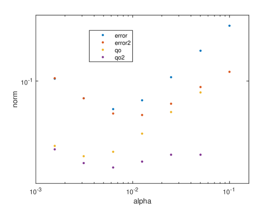
Figure 1: The quantities observed in a particular simulation: $\left\|x-x_{\alpha_{i}}^{\delta}\right\|$ (error), $\left\|x-\bar{x}_{\alpha_{i}}^{\delta}\right\|$ (error2), $\left\|x_{\alpha_{i}}^{\delta}-x_{\alpha_{i-1}}^{\delta}\right\|$ (qo), $\left\|\bar{x}_{\alpha_{i}}^{\delta}-\bar{x}_{\alpha_{i-1}}^{\delta}\right\|$ (qo2), plotted against the corresponding values of $\alpha_{i}$, $i=1,2,\ldots,7$.

References

• [1] R. Anderssen. The linear functional strategy for improperly posed problems. In J. R. Cannon and U. Hornung, editors, Inverse Problems, volume 77 of International Series of Numerical Mathematics, pages 11–30. Birkhäuser Basel, 1986.
• [2] R. S. Anderssen. On the use of linear functionals for Abel-type integral equations in applications. In F. De Hoog and M. A. Lukas, editors, The application and numerical solution of integral equations, pages 195–221. Sijthoff and Noordhof International Publishers, 1980.
• [3] R. S. Anderssen and H. W. Engl. The role of linear functionals in improving convergence rates for parameter identification via Tikhonov regularization. In M. Yamaguti et al., editor, Inverse Problems in Engineering Sciences, ICM-90, Satellite Conference Proceedings, pages 1–10. Springer, 1991.
• [4] A. B. Bakushinskii. Remarks on choosing regularization parameter using the quasi-optimality and ratio criterion. USSR Comp. Math. Math. Phys., 24:181–182, 1984.
• [5] F. Bauer, P. Mathé, and S. Pereverzev. Local solutions to inverse problems in geodesy. J. Geodesy, 81(1):39–51, 2007.
• [6] F. Bauer and M. Reiß. Regularization independent of the noise level: an analysis of quasi-optimality. Inverse Probl., 24(5):055009, 2008.
• [7] S. M. A. Becker. Regularization of statistical inverse problems and the Bakushinskii veto. Inverse Probl., 27(11):115010, 2011.
• [8] R. Bellman, B. G. Kashef, and J. Casti. Differential quadrature: a technique for the rapid solution of nonlinear partial differential equations. J. Comput. Phys., 10(1):40–52, 1972.
• [9] J. Chen, S. Pereverzyev Jr., and Y. Xu. Aggregation of regularized solutions from multiple observation models. Inverse Probl., 31(7):075005, 2015.
• [10] H. W. Engl and A. Neubauer. A parameter choice strategy for (iterated) Tikhonov regularization of ill-posed problems leading to superconvergence with optimal rates. Appl. Anal., 27:5–18, 1988.
• [11] A. Goldenshluger and S. V. Pereverzev. Adaptive estimation of linear functionals in Hilbert scales from indirect white noise observations. Probab. Theory Related Fields, 118(2):169–186, 2000.
• [12] U. Hämarik, R. Palm, and T. Raus. Comparison of parameter choices in regularization algorithms in case of different information about noise level. Calcolo, 48(1):47–59, 2011.
• [13] S. Kindermann and A. Neubauer. On the convergence of the quasioptimality criterion for (iterated) Tikhonov regularization. Inverse Probl. Imaging, 2(2):291–299, 2008.
• [14] J. Kusche and R. Klees. Regularization of gravity field estimation from satellite gravity gradients. J. Geodesy, 76(6):359–368, 2002.
• [15] A. S. Leonov. On the accuracy of Tikhonov regularizing algorithms and quasioptimal selection of a regularization parameter. Soviet Math. Dokl., 44:711–716, 1991.
• [16] A. K. Louis and P. Maass. A mollifier method for linear operator equations of the first kind. Inverse Probl., 6(3):427–440, 1990.
• [17] S. Lu and S. V. Pereverzev. Regularization theory for ill-posed problems: selected topics. Walter de Gruyter, 2013.
• [18] P. Mathé and S. V. Pereverzev. Direct estimation of linear functionals from indirect noisy observations. J. Complexity, 18(2):500–516, 2002.
• [19] A. Neubauer. The convergence of a new heuristic parameter selection criterion for general regularization methods. Inverse Probl., 24(5):055005, 2008.
• [20] R. Palm. Numerical Comparison of Regularization Algorithms for Solving Ill-Posed Problems. PhD thesis, Institute of Computer Science, University of Tartu, 2010.
• [21] A. N. Tikhonov and V. B. Glasko. Use of the regularization method in non-linear problems. USSR Comp. Math. Math. Phys., 5:93–107, 1965.