Perturbative width of open rigid strings

Abstract

We present a perturbative calculation of the energy profile width of rigid strings up to two loops in D dimensions. The perturbative expansion of the extrinsic-curvature term, signifying the rigidity/smoothness of the string in Polyakov-Kleinert action, is taken around the free Nambu-Goto string. The mean-square width of the string field is derived for open strings with the Dirichlet boundary condition. We compare the broadening of the smooth Polyakov-Kleinert string to the lattice Monte Carlo data of the QCD flux tube just before the deconfinement point and find a good match at the intermediate and large color source separation.

I Introduction

The confinement of quarks is an outstanding feature of quantum chromodynamics (QCD). An analytic proof of color confinement in any non-Abelian gauge theory remains a far-reaching goal. Nevertheless the confinement property can be probed numerically in the simulations of the bound state of infinitely heavy quark-antiquark ($Q\bar{Q}$) which have shown the linearly rising property of the static potential 1 ; 2 ; 3 ; 4 ; 5 ; 6 ; 7 ; 8 ; 9 .

The linear increase in the $Q\bar{Q}$ potential is compatible with the creation of a stringlike object that connects the color sources. In a string model Luscherfr ; Luscher:2002qv of confinement, the chromoelectric flux tubes are squeezed into a narrow region forming a stringlike tube by the dual Meissner effect tHooft ; 'tHooft:1999au ; Mandelstam76 ; Bali1996 ; Carmona:2001ja ; DiGiacomo:1999a ; DiGiacomo:1999b . String formation is observed in many strongly correlated systems  PhysRevB.78.024510 ; 2007arXiv0709.1042K ; Nielsen197345 ; Lo:2005xt and is often characterized by a roughening phase in which oscillations transverse to the classical world sheet result in universal effects. These effects are detectable in numerical simulations of lattice gauge theories (LGTs) Juge:2002br ; HariDass2008273 ; Caselle:2016mqu ; caselle-2002 ; Pennanen:1997qm ; Brandt:2016xsp . The Lüscher term is the first universal correction to the linearly rising $Q\bar{Q}$ potential, and its analog in the baryonic three-quark system is the Lüscher-like term Jahn2004700 ; deForcrand:2005vv .

The confining string is an idealized one-dimension bosonic string providing a low-energy effective description of the confining flux-tube Luscherfr ; Luscher:2002qv ; PhysRevLett.67.1681 that is valid at distance scales larger than the width of the tube Caselle:2012rp . The stringlike object breaks the rotational and translational symmetry of the Yang-Mills vacuum, leading to the generation of spontaneous Goldstone modes GODDARD1973109 ; Low:2001bw . Study of the collective modes profile of the free Nambu-Goto (NG) string has pointed out another universal feature in conjunction with the Lüscher term of the string potential, which is the logarithmic broadening of the width of the energy profile with the increase of the string length Luscher:1980iy . The broadening of the free string is expected to turn into a linear pattern before deconfinement is reached from below  allais ; Gliozzi:2010zv ; Caselle:2010zs ; Gliozzi:2010jh at large color separations.

The energy profile between the confined color charges and the characteristic broadening is a key source for delving into the physics of the confining force from the first principles. The energy-density profile is a more challenging quantity to measure on the lattice compared to the $Q\bar{Q}$ potential. The exponentially decaying field correlators involve an additional term of the field strength tensor PhysRevD.82.094503 ; Bakry:2010sp ; Bicudo:2017uyy ; deForcrand:2005vv that brings about substantial numerical effort in certain gauge groups.

The expansion of computational resources and the constant enhancement of resolution power have opened up a plethora of prospects to examine the energy profile features of confined bound states. Many lattice simulations of different gauge groups, for example, have unambiguously confirmed the predicted logarithmic broadening of confined strings and their linear behavior at finite temperatures and large distances  Caselle:1995fh ; Bonati:2011nt ; Caselle:2021eir ; HASENBUSCH1994124 ; Caselle:2006dv ; Bringoltz:2008nd ; Athenodorou:2008cj ; Juge:2002br ; HariDass:2006pq ; Giudice:2006hw ; Bonati:2021vbc ; Luscher:2004ib ; Pepe:2010na .

Nevertheless, the analysis of the string’s fine structure in the lattice numerical data for the broadening profile reveals substantial deviations PhysRevD.82.094503 ; Bakry:2010sp ; Bicudo:2017uyy from the free string NG model in the intermediate length scale at high temperatures. The excited spectrum Luscher:2004ib and the finite temperature string tension  Pisarski ; PhysRevD.85.077501 ; Kac obtained from the Gaussian partition function of the free NG action shows a similar disagreement with the numerical data  Juge:2002br ; Kac ; Bakry:2010sp ; Bakry:2017utr for large color separation.

Higher-order corrections to the NG action  PhysRevD.27.2944 ; Aharony:2010cx ; Billo:2012da have been extensively investigated numerically to establish their relevance in each gauge model Caselle:2004jq ; Caselle:2004er ; Pepe:2010na ; Gliozzi:2010zv . Indeed, there is no evidence that all orders of power expansion are universal Alvarez:1981kc ; Arvis:1983fp .

Different model-dependent effective strings Caselle:2004jq may be identified in the numerical simulations of peculiar gauge groups. For instance, neither Abelian $Z(2)$ nor non-Abelian $SU(2)$ and $SU(3)$ confining gauge models have any universal properties in common, other than the Lüscher term, at the next-to-leading-order operator Caselle:2004jq . The 3D percolation model  Giudice:2009di has likewise a term that deviates from the universal behavior. At next-to-leading order (NLO), deviations from the NG string are detected in the simulations of non-Abelian $SU(3)$ Yang-Mills theory in 4D  Bakry:2017utr ; Bakry:2018kpn ; Bakry:2020ebo ; Bakry:2020flt .

Along with the boundary corrections Billo:2012da ; Bakry:2020ebo ; Brandt:2010bw ; Bakry and the global geometrical characteristics of the flux tubes Bakry:2020akg ; Dubovsky , to gain insight into structure of strings  Ambjorn:2014rwa , one is tempted to investigate likewise the putative physical implications of the local geometries POLYAKOV19 ; Kleinert:1986bk in the string action  Caselle:2014eka ; Brandt:2017yzw ; Brandt:2021kvt .

Simulations of the ground state of the Y-shaped flux tubes Okiharu:2003vt ; Bissey:2006bz ; Okiharu:2004ve ; Okiharu:2004wy ; Bicudo:2011hk point to absence of acute or sharp angles among strings. The ground state of three-quark potential is minimized while tuning (in Wilson loop overlap formalism) a system of spatial Y-shaped gauge links with equal angles of $120^{\circ}$ at the junction, as shown by Bissey et al. Bissey:2006bz . This obviously follows from a tension that prefers $120^{\circ}$ angles at the junctions to balance the three forces along the string (even at high temperature Bakry:2011kga ; Bakry:2014gea ; Bakry:2016uwt ). On the other-hand, L and T-shaped strings decouple by the evolution of Euclidean time Bissey:2006bz indicating that other angles among strings correspond to higher excited states. These geometrical observations highlight the interconnection between energy of the string’s configurations and the steepness of both the fluctuations and self-intersection along one single string.

The interpretation of the string’s stiffness may be relevant to the string’s vortex line picture  Langfeld:2002vy , or other self-interactions of the string  PhysRevD.51.1842 . The consideration of geometric-dependent quantities in the string action could show some pertinence to the characteristics of the confining flux tubes, in particular at intermediate distances and high temperatures or for the excited states.

To realize the rigidity property mathematically the string action is considered using a Poincare-invariant term proportional to the extrinsic-curvature of the string’s world sheet. Some years ago, Polyakov POLYAKOV19 and Kleinert Kleinert:1986bk proposed this intriguing generalization to stabilize the NG string action. In this model, the area, as well as the geometrical layout of the embedded sheet in space-time, affect the surface representation of the Polyakov-Kleinert (PK) string. That is, following the NG action, the bosonic free-string action is equipped with an additional term of extrinsic-curvature as a next-order operator POLYAKOV19 ; Kleinert:1986bk .

The PK string theory, like the ordinary NG string, yields a QCD model of smooth flux sheets across long-distance scales, but with abruptly creased surfaces filtered out. This is handled by the extrinsic-curvature term’s leading parameter, which promotes smooth string configurations over those that are sharply curved.

The model is relevant to QCD main features with ultraviolet (UV) freedom and infrared (IR) confinement properties  POLYAKOV19 ; Kleinert:1986bk and is consistent with glueball formation  Kleinert:1988hz ; Viswanathan:1987et , in addition to a real $Q\bar{Q}$ potential German:1989vk ; Nesterenko1992 ; Ambjorn:2014rwa and a possible tachyonic-free spectrum above some critical coupling Viswanathan:1987et .

The adiabatic and nonrelativistic limit of the Isgur-Paton model Isgur , inspired from the Hamiltonian LGT formulation in the strong coupling, corresponds to glueballs conjectured as rings of glue held together by a string tension equal to the $Q\bar{Q}$ potential, with “rapid” transverse oscillations and “slow” radial excitation. The stiff glueball model, on the other hand, hypothesizes glueballs as a superposition of flux rings generated by a closed chain of gluons with certain momenta Caselle:2013qpa ; Johnson:2000qz ; Dubovsky:2016cog . The partition function is that of closed smooth string on genus-one Riemann surfaces in Euclidean space, where the strings have extrinsic-curvature and spontaneously generated tension capable of forming glueballs. The PK model’s parameters have a physical origin in QCD as a consequence of the gluonic degrees of freedom’s complex dynamics. Even in the absence of quarks, QCD enables the development of a flux tube with a single length scale entering both the string tension and the thickness of the tube Kleinert:1988hz ; Viswanathan:1987et .

With these attractive features, the theory induced a research effort to reveal the relevant properties such as its perturbative stability in critical dimensions PhysRevLett.58.1300 , the dynamical generation of the string tension Kleinert:1988vq , and the exact potential in the large dimension limit Braaten:1987gq ; Kleinert:1989re . This is in addition to the relevant thermodynamic characteristics such as the deconfinement transition point Kleinert:1987kv , partition function Elizalde:1993af , free energy and string tension at finite temperature Viswanathan:1988ad ; German:1991tc ; Nesterenko:1997ku .

Recently, rigid-string effects have been reported in the numerical simulations of the confining potential Abelian $U(1)$ compact gauge group Caselle:2014eka ; Caselle:2016mqu . The rigidity effects in the confining potential are significant in reducing the deviations from the NG string for temperatures just before deconfinement in the quenched QCD  Bakry:2017utr ; Bakry:2018kpn ; Bakry:2020ebo ; Bakry:2020flt . Manifestation of stiffness in the IR region of non-Abelian $SU(N)$ gauge theories in 3D has been reported in Ref. Brandt:2017yzw .

For many QCD processes tractable to stringy portrayals, disclosing the characteristics of the flux tube model beyond the Nambu-Goto arrangement could be demanding. This is especially true for high-energy processes Caselle:2015tza ; GIDDINGS198955 like the Hagedorn spectrum and glueballs thermodynamics Caselle:2013qpa ; Johnson:2000qz , string fireballs Kalaydzhyan:2014tfa and mesonic spectroscopy Bali:2013fpo ; Kalashnikova:2002zz ; Grach:2008ij ; GIDDINGS198955 .

The energy chart features of the smooth flux sheets remained ambiguous despite substantial discussion of stiffness at the level of static quark potential Kleinert:1988hz ; Viswanathan:1987et ; German:1989vk ; Nesterenko1992 ; Ambjorn:2014rwa ; Kleinert:1988vq ; Braaten:1987gq ; Kleinert:1989re ; German:1991tc ; Nesterenko:1997ku . This, together with the resurgent interest in examining smooth strings on the lattice Caselle:2014eka ; Caselle:2016mqu ; Brandt:2017yzw , calls for extending the discussion of the string’s rigidity effects on the characteristics of the energy field within hadronic bound states.

The goal of this study is to lay out an analytical form for the smooth string mean-square width that is practically viable for numerical models. The calculations described here are for an open string on a cylinder with the Dirichlet boundary condition, which is compatible with energy fields in static mesonic setups. In light of recent lattice studies Caselle:2014eka ; Caselle:2016mqu ; Brandt:2017yzw that show the delicate manifestation of smooth strings in the IR region of Abelian and non-Abelian gauge models, the mean-square width corrections due to the geometric term in PK action are perturbatively evaluated around the free NG solution.

In Sec.II and III, we consider the perturbative expansion of the extrinsic-curvature term and evaluate the width of the leading- and next-to-leading order approximations expanded beyond the free NG string width, respectively. In Sec.IV we discuss the behavior of the solution with the corresponding fits to lattice Monte Carlo data. We provide the concluding remarks in Sec.V.

II Width of Rigid String in Leading-order Approximation

Several physical IR properties of the string’s world sheet are in agreement with what is expected for a QCD flux tube at low temperatures. In the IR limit, the dynamics of the flux tube follow toward a massless and free-string theory; for large enough color source separation, an effective field theory with infrared action can be prescribed as

$$\begin{split}S[\mathbf{X}]=&S_{\rm{cl}}+S_{0}[\mathbf{X}]\\ =&\sigma R~{}L_{T}+\dfrac{1}{2}\int d\zeta_{0}\int d\zeta\left(\dfrac{\partial\mathbf{X}}{\partial\zeta_{\alpha}}\cdot\dfrac{\partial\mathbf{X}}{\partial\zeta_{\alpha}}\right),\end{split}$$ (1)

where $S_{cl}$ is the classical configuration or perimeter-area term, the coordinates $\zeta_{0}$ and $\zeta$ parameterize the world sheet ($\alpha=0,1$), the vector $X^{\mu}(\zeta_{0},\zeta)$ in the transverse gauge describes the fluctuations of the two-dimensional bosonic world sheet relative to the surface of minimal-area/the classical configuration with $(\mu=1,2,...,d-2)$ and the action $S_{0}[\mathbf{X}]$ is known as the Gaussian term. The above action $S[\mathbf{X}]$, Eq.(1), is referred to as the free bosonic string action.

The free bosonic string theory can be obtained from the truncated perturbative expansion of the NG string action. The NG string action is the simplest possible action that is proportional to the world sheet area

$$S^{\rm{NG}}=\frac{1}{2}\int d^{2}\zeta\sqrt{g}g^{\alpha\beta}\frac{\partial\mathbf{X}}{\partial\zeta_{\alpha}}\cdot\frac{\partial\mathbf{X}}{\partial\zeta_{\beta}},$$ (2)

where $g^{\alpha\beta}$ is the intrinsic metric induced on the two-dimensional world sheet, parametrized by $X_{\mu}(\zeta)$ embedded in the background $R^{D}$.

$$g^{\alpha\beta}=\frac{\partial\mathbf{X}}{\partial\zeta_{\alpha}}\cdot\frac{\partial\mathbf{X}}{\partial\zeta_{\beta}},~{}~{}~{}~{}(\alpha,\beta=1,2,....,D-2),~{}~{}~{}~{}g={\rm{det}}(g^{\alpha\beta}).$$ (3)

The Dirichlet boundary condition, corresponding to fixed displacement vector at the ends $\zeta=0$ and $\zeta=R$, and periodic boundary condition in time $\zeta_{0}$ with period $L_{T}=1/T$, proportional to inverse temperature scale. For string tension $\sigma$ and classical area of an open-string world sheet given by $A=L_{T}R$ the NG action $S^{\rm{NG}}$ can be expanded  Giudice:2009di in a natural dimensionless parameter $\left(\frac{1}{\sigma A}\right)$ such that

$$\begin{split}S^{\rm{NG}}[\mathbf{X}]&=S_{\rm{cl}}+S_{0}[\mathbf{X}]+S_{1}[\mathbf{X}]+...\\ &=S_{\rm{cl}}+S_{0}[\mathbf{X}]\\ &\scalebox{0.85}{\mbox{$\displaystyle+\dfrac{1}{\sigma A}\int\int d\zeta_{0}d\zeta\Bigg{[}\left(\dfrac{\partial\mathbf{X}}{\partial\zeta_{\alpha}}\cdot\dfrac{\partial\mathbf{X}}{\partial\zeta_{\alpha}}\right)^{2}+\left(\dfrac{\partial\mathbf{X}}{\partial\zeta_{\alpha}}\cdot\dfrac{\partial\mathbf{X}}{\partial\zeta_{\beta}}\right)^{2}\Bigg{]}$}}\\ &+\mathcal{O}\bigg{(}\dfrac{1}{(\sigma A)^{2}}\bigg{)}.\end{split}$$ (4)

The above expression is an effective low-energy expansion of the string action with truncation that holds in the long string limit. Switching from the physical units  Luscher:2004ib of the bosonic fields to dimensionless form $\frac{\mathbf{X}}{\sqrt{\sigma}}\rightarrow\mathbf{X}$ the leading-order (LO) and the NLO terms of NG action after field redefinition can be written as

$$\begin{split}S^{\rm{NG}}_{\ell o}[\mathbf{X}]&=\sigma R~{}L_{T}+\frac{\sigma}{2}\int d\zeta_{0}\int d\zeta\left(\frac{\partial\mathbf{X}}{\partial\zeta_{\alpha}}\cdot\frac{\partial\mathbf{X}}{\partial\zeta_{\alpha}}\right),\\ S^{\rm{NG}}_{n\ell o}[\mathbf{X}]&=\sigma\int d\zeta_{0}\int d\zeta\left[\left(\frac{\partial\mathbf{X}}{\partial\zeta_{\alpha}}\cdot\frac{\partial\mathbf{X}}{\partial\zeta_{\alpha}}\right)^{2}+\left(\frac{\partial\mathbf{X}}{\partial\zeta_{\alpha}}\cdot\frac{\partial\mathbf{X}}{\partial\zeta_{\beta}}\right)^{2}\right].\end{split}$$ (5)

The action of the PK bosonic string with the extrinsic-curvature term reads as

$$S^{\rm{PK}}[\mathbf{X}]= S^{\rm{NG}}[\mathbf{X}]+S^{\rm{Ex}},$$ (6)

$$= S^{\rm{NG}}[\mathbf{X}]+\alpha_{r}\int d^{2}\zeta\sqrt{g}\Delta\mathbf{X}\cdot\Delta\mathbf{X},$$

with the parameter $\alpha_{r}$ referring to the rigidity factor and the $\triangle$ operator given by

$$\triangle\equiv(1/\sqrt{g})\partial_{\alpha}(\sqrt{g}g^{\alpha\beta}\partial_{\beta}).$$ (7)

The second term proportional to the extrinsic-curvature circumvents the undesirable features of the NG action such as ghost, tachyons, and an imaginary static potential between quarks when the distance becomes smaller than some critical distance POLYAKOV19 ; Kleinert:1986bk ; Kleinert:1988hz ; Viswanathan:1988ad ; German:1989vk ; Nesterenko1992 ; Ambjorn:2014rwa .

A similar argument can be used to expand the terms proportional to the extrinsic-curvature

$$S^{\rm{Ext}}[\mathbf{X}] =\left(S^{(1)}+S^{(2)}\right)+....$$ (8)

$$\scalebox{0.75}{\mbox{$\displaystyle-\frac{\alpha_{r}}{2}\left(\frac{\partial\mathbf{X}}{\partial\zeta_{\alpha}}\cdot\frac{\partial^{2}\mathbf{X}}{\partial\zeta_{\beta}^{2}}\right)^{2}-\alpha_{r}\left(\frac{\partial\mathbf{X}}{\partial\zeta_{\alpha}}\cdot\frac{\partial\mathbf{X}}{\partial\zeta_{\beta}}\right)\left(\frac{\partial^{2}\mathbf{X}}{\partial\zeta_{\alpha}\partial\zeta_{\beta}}\cdot\frac{\partial^{2}\mathbf{X}}{\partial\zeta_{\gamma}^{2}}\right)+..\Bigg{]}$}}.$$

The mean-squared width of the string is defined as the second moment of the field with respect to the center of mass of the string $X_{0}$ and is given by

$$W^{2}(\zeta)=\frac{\int DX(\mathbf{X}(\zeta,\zeta_{0})-\mathbf{X_{0}})^{2}e^{-S^{\rm{PK}}[\mathbf{X}]}}{\int DXe^{-S^{\rm{PK}}[\mathbf{X}]}}.$$ (9)

In the truncated form the PK string action reads

$$S^{\rm{PK}}[\mathbf{X}]\approx S^{\rm{NG}}_{\ell o}[\mathbf{X}]+S^{\rm{Pert}}[\mathbf{X}],$$ (10)

with the general perturbation series

$$S^{\rm{Pert}}[\mathbf{X}]=S^{\rm{NG}}_{n\ell o}+...+\left(S^{(1)}+S^{(2)}\right)+....$$ (11)

In the following, we calculate the width of the rigid string Eq.(9), considering the first term in the perturbative expansion $S^{(1)}$ of the Polyakov extrinsic-curvature term given by

$$S^{(1)}=\alpha_{r}\int_{0}^{L_{T}}d\zeta_{0}\int_{0}^{R}d\zeta\left[\left(\frac{\partial^{2}\mathbf{X}}{\partial\zeta^{2}}\right)^{2}+\left(\frac{\partial^{2}\mathbf{X}}{\partial\zeta_{0}^{2}}\right)^{2}\right].$$ (12)

In the next section, we evaluate the width at the NLO in the extrinsic-curvature term $S^{(2)}$ given in Eq.(8). Expanding around the free-string action Eq.(1), the squared width of the string  Gliozzi:2010zt is

$$W^{2}(\zeta) =W_{\rm{NG_{(\ell o)}}}^{2}(\zeta)-\langle\mathbf{X}^{2}(\zeta,\zeta_{0})S^{\rm{Pert}}\rangle_{0}$$ (13)

$$+2\theta\langle\partial_{\alpha}\mathbf{X}^{2}(\zeta,\zeta_{0})\rangle_{0}+\theta^{2}\langle\partial_{\alpha}^{2}\mathbf{X}^{2}(\zeta,\zeta_{0})\rangle_{0}$$

$$-\frac{\theta^{2}}{L_{T}R}\int d\zeta_{0}~{}d\zeta~{}d\zeta^{\prime}_{0}~{}d\zeta^{\prime}\langle\partial_{\alpha}^{2}\mathbf{X}(\zeta,\zeta_{0})\textperiodcentered\partial_{\alpha^{\prime}}^{2}\mathbf{X}(\zeta,\zeta^{{}^{\prime}}_{0})\rangle_{0},$$

where the vacuum expectation value $\langle...\rangle_{0}$ is with respect to the free-string partition function, $\theta$ is an effective low-energy parameter, and $L_{T}$ is the length of compactified time direction for the cylindrical boundary condition.

Substituting Eq.(8) in the expansion Eq.(13), the mean-square width reads

$$\scalebox{0.8}{\mbox{$\displaystyle W^{2}(R,L_{T})=W^{2}_{\rm{NG_{(\ell o)}}}(R,L_{T})+W^{2}_{\rm{NG_{(n\ell o)}}}(R,L_{T})+W^{2}_{\rm{Ext}}(R,L_{T})$}},$$ (14)

with

$$W^{2}_{\rm{NG_{(n\ell o)}}}(R,L_{T})=-\left\langle\mathbf{X}^{2}(\zeta,\zeta_{0})S^{\rm{NG}}_{n\ell o}\right\rangle,$$ (15)

and

$$W^{2}_{\rm{Ext}}(R,L_{T}) =-\left\langle\mathbf{X}^{2}(\zeta,\zeta_{0})(S^{(1)}+S^{(2)})\right\rangle$$ (16)

$$=W^{2}_{\rm{Ext_{(\ell o)}}}(R,L_{T})+W^{2}_{\rm{Ext_{(n\ell o)}}}(R,L_{T}).$$ (17)

Let us define the Green’s function $G(\mathbf{\zeta;\zeta^{\prime}})=\langle\mathbf{X}(\zeta,\zeta_{0})\mathbf{X}(\zeta^{{}^{\prime}},\zeta^{{}^{\prime}}_{0})\rangle$ as the two-point Gaussian propagator. The correlator on a cylindrical sheet Gliozzi:2010zt of surface area $RL_{T}$ is given by

$$G(\mathbf{\zeta;\zeta^{\prime}}) =\frac{1}{\pi\sigma}\sum_{n=1}^{\infty}\frac{1}{n\left(1-q^{n}\right)}\sin\left(\frac{\pi n\zeta}{R}\right)\sin\left(\frac{\pi n\zeta^{\prime}}{R}\right)$$

$$~{}~{}~{}\scalebox{0.9}{\mbox{$\displaystyle\times\left(q^{n}e^{\frac{\pi n(\zeta_{0}-\zeta^{{}^{\prime}}_{0})}{R}}+e^{-\frac{\pi n(\zeta_{0}-\zeta^{{}^{\prime}}_{0})}{R}}\right)$}},$$ (18)

where $q=e^{-\pi\frac{L_{T}}{R}}$ is the complementary nome. The Dirichlet boundary condition  Gliozzi:2010zt is encoded in the above propagator.

After some algebraic manipulations and using the following auxiliary identities

$$\xi_{j}=\begin{cases}-i\frac{\pi}{2R}(\zeta_{0}^{{}^{\prime}}-\zeta_{0}+(-1)^{j}i\zeta-i\zeta^{\prime}-L_{T}),&\mbox{for }~{}j=1,2\\ -i\frac{\pi}{2R}(\zeta_{0}^{{}^{\prime}}-\zeta_{0}+(-1)^{j}i\zeta+i\zeta^{\prime}-L_{T}),&\mbox{for }~{}j=3,4\\ \end{cases}$$ (19)

the correlator Eq.(18) can be recast into the following closed form:

$$G(\xi)=\frac{1}{4\pi\sigma}\log\left[\frac{\vartheta_{4}(\xi_{1},q)\vartheta_{4}(\xi_{4},q)}{\vartheta_{4}(\xi_{2},q)\vartheta_{4}(\xi_{3},q)}\right],$$ (20)

where $\vartheta_{4}\left(\xi,q\right)$ is the Jacobi theta function.

The expectation value of the free NG string can be derived from the above form using Jacobi triple product formula. The mean-square width of the noninteracting string at the middle plane perpendicular to the string is

$$W^{2}_{NG_{(\ell o)}}(R/2) =\lim_{\epsilon\rightarrow 0}G(\mathbf{\zeta;\zeta^{\prime}}),$$

$$=\frac{D-2}{4\pi\sigma}\log\left[\frac{\vartheta_{3}(0,\sqrt{q})}{\vartheta_{4}(0,\sqrt{q})}\right]+R_{0}^{2},$$ (21)

with $R_{0}^{2}$ as the regularization scale, (see Appx.(B) for details). The above formula can be pinned down through the standard relations between the elliptic Jacobi and Dedekind $\eta$ functions to an equivalent to either of the forms derived in Refs.allais ; Gliozzi:2010zt .

The first term in Eq.(17) representing the LO perturbation due to the smooth string in terms of the corresponding Green’s functions is

$$W^{2}_{\rm{Ext_{(\ell o)}}} =-(D-2)\alpha_{r}\lim_{\begin{subarray}{c}\epsilon^{\prime}\to 0\\ \epsilon\to 0\end{subarray}}\int_{0}^{R}d\zeta^{\prime}\int_{0}^{L_{T}}d\zeta^{\prime}_{0}\Big{[}G(\mathbf{\zeta;\zeta^{\prime}})\partial_{\alpha}^{2}\partial_{\alpha^{\prime}}^{2}G(\mathbf{\zeta^{\prime};\zeta})$$

$$~{}~{}~{}~{}~{}~{}~{}~{}~{}~{}~{}~{}~{}~{}~{}~{}~{}~{}~{}~{}~{}~{}~{}~{}~{}~{}~{}~{}~{}~{}~{}~{}~{}~{}\scalebox{0.8}{\mbox{$\displaystyle+\partial_{\alpha}^{2}G(\mathbf{\zeta;\zeta^{\prime}})\partial_{\alpha^{\prime}}^{2}G(\mathbf{\zeta^{\prime};\zeta})\Big{]}$}}.$$ (22)

The limit, $\epsilon,\epsilon^{\prime}\to 0$, is such that the integral is ultimately regularized by the point-split method. Therefore, one may recast Eq.(II) as

$$\scalebox{0.9}{\mbox{$\displaystyle W_{\rm{Ext_{(\ell o)}}}^{2}=\frac{-\pi(D-2)\alpha_{r}}{4R^{2}\sigma^{2}}\sum_{n=1}^{\infty}\sum_{m=1}^{\infty}\left(q^{m}+1\right)^{2}q^{-m}\frac{n\left(q^{n}+1\right)}{\left(q^{n}-1\right)}$}}.$$ (23)

With the use of the Riemann $\zeta$ function regularization of the divergent sums in Eq.(23), a generic form for the contribution of the extrinsic-curvature term to the mean-square width can be extracted as

$$W_{\rm{Ext_{(\ell o)}}}^{2}=\frac{-\pi(D-2)\alpha_{r}}{24R^{2}\sigma^{2}}E_{2}\left(\tau\right).$$ (24)

Using the standard modular transform of an Eisenstein series Zagier2008 ; Freitag2009

$$E_{2}\left(\tau\right)=\frac{-4R^{2}}{L_{T}^{2}}E_{2}\left(\frac{1}{\tau}\right)+\frac{6}{i\pi\tau}.$$ (25)

The contribution of the rigidity term to the mean-square width of the string at the limit $R\gg L_{T}$ can be read off from Eq.(24),

$$W_{\rm{Ext_{(\ell o)}}}^{2}=-\left(\frac{(D-2)\alpha_{r}}{2\sigma^{2}RL_{T}}\right)+C(L_{T}),$$ (26)

with $C(L_{T})$ being only a function in the thermodynamic scale, see Appx.(C) for details.

III The Interaction-term Contribution to the Width

In the following, we evaluate the NLO term in the perturbation expansion German:1989vk of the extrinsic-curvature of rigid string $S^{(2)}$ of the PK action Eq.(8), which is given by

$$S^{(2)} =\int_{0}^{L_{T}}d\zeta_{0}\int_{0}^{R}d\zeta\Bigg{[}\frac{\sigma}{8}\left(\frac{\partial\mathbf{X}}{\partial\zeta_{\alpha}}\right)^{4}-\frac{\sigma}{4}\left(\frac{\partial\mathbf{X}}{\partial\zeta_{\alpha}}\cdot\frac{\partial\mathbf{X}}{\partial\zeta_{\beta}}\right)^{2}$$

$$~{}~{}~{}~{}~{}~{}~{}~{}+2\alpha_{r}\left(\frac{\partial^{2}\mathbf{X}}{\partial\zeta_{\alpha}^{2}}\right)^{2}\left(\frac{\partial\mathbf{X}}{\partial\zeta_{\beta}}\right)^{2}-\frac{\alpha_{r}}{2}\left(\frac{\partial\mathbf{X}}{\partial\zeta_{\alpha}}\cdot\frac{\partial^{2}\mathbf{X}}{\partial\zeta_{\beta}^{2}}\right)^{2}$$

$$~{}~{}~{}~{}~{}~{}~{}~{}-\alpha_{r}\left(\frac{\partial\mathbf{X}}{\partial\zeta_{\alpha}}\cdot\frac{\partial\mathbf{X}}{\partial\zeta_{\beta}}\right)\left(\frac{\partial^{2}\mathbf{X}}{\partial\zeta_{\alpha}\partial\zeta_{\beta}}\cdot\frac{\partial^{2}\mathbf{X}}{\partial\zeta_{\gamma}^{2}}\right)\Bigg{]}.$$

Using notation from Ref.German:1989vk one can write the contribution to a width of the stiff string due to second loop interactions in the following series:

$$W^{2}_{\rm{Ext_{(n\ell o)}}} =\left\langle\mathbf{X}^{2}S^{(2)}\right\rangle$$

$$=\left\langle\mathbf{X}^{2}\left(S^{(2)}_{(a)}+S^{(2)}_{(b)}+S^{(2)}_{(c)}+S^{(2)}_{(d)}+S^{(2)}_{(e)}\right)\right\rangle.$$ (28)

Here each expectation value is written with respect to the free NG string and corresponds to the respective term in Eq.(III). The first two interaction terms have the dimensional coupling $\sigma$ with the Feynman diagrams corresponding to disconnected loops shown in Fig.1.

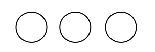
Figure 1: Feynman diagrams corresponding to disconnected loops German:1989vk of the first two terms of NLO expansion, Eq.(28).

After Wick contraction German:1989vk , the first interaction term in Eq.(28) reads

(29)

$$~{}~{}~{}~{}~{}~{}~{}~{}~{}~{}~{}~{}~{}\scalebox{0.8}{\mbox{$\displaystyle+\left\langle\mathbf{X}^{2}\right\rangle_{0}\left\langle\frac{\partial\mathbf{X}}{\partial\zeta_{\alpha}}\frac{\partial\mathbf{X}}{\partial\zeta_{\beta}}\right\rangle_{0}\left\langle\frac{\partial\mathbf{X}}{\partial\zeta_{\alpha}}\frac{\partial\mathbf{X}}{\partial\zeta_{\beta}}\right\rangle_{0}\Bigg{)}\Bigg{]}$}}.$$

The above correlator upon point split becomes an integral over the sum of the triple product of derivatives of Green’s functions

(30)

$$~{}~{}~{}~{}~{}~{}~{}~{}~{}~{}~{}~{}\scalebox{0.75}{\mbox{$\displaystyle+G\left(\mathbf{\zeta;\zeta^{\prime}}\right)\partial_{\alpha^{\prime}}\partial_{\beta^{\prime\prime}}G\left(\mathbf{\zeta^{\prime};\zeta^{\prime\prime}}\right)\partial_{\alpha^{\prime\prime}}\partial_{\beta}G\left(\mathbf{\zeta^{\prime\prime};\zeta}\right)\bigg{)}\Bigg{]}d\zeta d\zeta_{0}$}}.$$ (31)

The second Wick-contracted interaction term in Eq.(28) reads

$$\left\langle\mathbf{X}^{2}S_{(b)}\right\rangle_{0} =\frac{-\sigma}{4}\left\langle\mathbf{X}\cdot\mathbf{X}\left(\frac{\partial\mathbf{X}}{\partial\zeta_{\alpha}}\cdot\frac{\partial\mathbf{X}}{\partial\zeta_{\beta}}\right)^{2}\right\rangle_{0}$$

$$~{}~{}~{}~{}~{}~{}~{}~{}~{}~{}~{}~{}~{}~{}~{}~{}~{}\scalebox{0.75}{\mbox{$\displaystyle+\left\langle\frac{\partial\mathbf{X}}{\partial\zeta_{\alpha}}\frac{\partial X}{\partial\zeta_{\beta}}\right\rangle_{0}\left\langle\mathbf{X}\frac{\partial\mathbf{X}}{\partial\zeta_{\alpha}}\right\rangle_{0}\left\langle\mathbf{X}\frac{\partial\mathbf{X}}{\partial\zeta_{\beta}}\right\rangle_{0}\bigg{)}\Bigg{]}$}}.$$

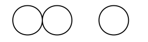
Figure 2: Connected and disconnected loops corresponding to the interaction terms $\left\langle\mathbf{X}^{2}S^{(2)}_{(c)}\right\rangle$, $\left\langle\mathbf{X}^{2}S^{(2)}_{(d)}\right\rangle$ and $\left\langle\mathbf{X}^{2}S^{(2)}_{(e)}\right\rangle$ in Eq.(28) with dimensionless couplings $\alpha_{r}$.

The sum of the corresponding Green’s correlators is given by

(33)

$$~{}~{}~{}~{}~{}~{}~{}~{}~{}\scalebox{0.85}{\mbox{$\displaystyle+G\left(\mathbf{\zeta;\zeta^{\prime}}\right)\partial_{\alpha^{\prime}}\partial_{\beta^{\prime\prime}}G\left(\mathbf{\zeta^{\prime};\zeta^{\prime\prime}}\right)\partial_{\alpha^{\prime\prime}}\partial_{\beta}G\left(\mathbf{\zeta^{\prime\prime};\zeta}\right)\bigg{)}\Bigg{]}d\zeta d\zeta_{0}$}}.$$ (34)

The above two correlators are given by the sum of the Green’s triple product and the remaining integrals vanish (see Appx.(D) for detailed calculations),

$$I^{(2)}_{1}(R,L_{T})$$ (35)

and

$$I^{(2)}_{2}(R,L_{T})$$ (36)

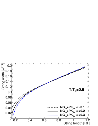
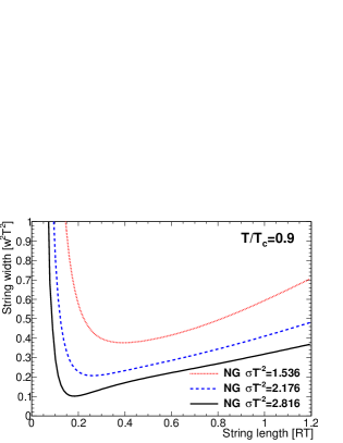
Figure 3: The mean-square width of the string, $W^{2}(\frac{R}{2})$, at the middle plane versus the string length $R$. The temperature scales $T/T_{c}$ mimics a Yang-Mills theory at $\beta=6$.0 PhysRevD.85.077501 . (a) The plot compares $W^{2}=W^{2}_{\rm{NG_{(\ell o)}}}$ of the free NG string Eq.(21) and the corresponding square width of PK string $W^{2}=W^{2}_{\rm{NG_{(\ell o)}}}+W^{2}_{\rm{NG_{(n\ell o)}}}+W^{2}_{\rm{Ext_{(\ell o)}}}$ given by Eq.(24) at one loop in extrinsic-curvature, at the standard value Schilling93 of string tension $\sqrt{\sigma}=440$ MeV. (b) Two-loop mean-square width of pure NG string Eqs.(21) and (38), plotted versus the string length for each depicted value of $\sigma T^{-2}$.

The sum of the first two interaction terms with the dimensional weights yields the NLO term (15) of the pure NG action

$$W^{2}_{NG_{(n\ell o)}}=\left((D-2)^{2}-(D-2)\right)I^{(2)}_{1}+(D-2)I^{(2)}_{2}.$$ (37)

The integrals of Eqs.(122) and (123) have been worked out in detail in Ref. Gliozzi:2010zt . The NLO correction to the width of the NG string then reads

$$W^{2}_{NG_{(n\ell o)}} =\frac{\pi}{12\sigma R^{2}}\Big{[}E_{2}(\tau)-4E_{2}(2\tau)\Big{]}\left(W_{lo}^{2}-\frac{D-2}{4\pi\sigma}\right)$$

$$\scalebox{0.7}{\mbox{$\displaystyle+\frac{(D-2)\pi}{12\sigma^{2}R^{2}}\Bigg{\{}\tau\Big{(}q\frac{d}{dq}-\frac{D-2}{12}E_{2}(\tau)\Big{)}\Big{[}E_{2}(2\tau)-E_{2}(\tau)\Big{]}-\frac{D-2}{8\pi}E_{2}(\tau)\Bigg{\}}$}},$$

with $\tau=\frac{iL_{T}}{2R}$ as the modular parameter of the cylindrical sheet.

The next three interaction terms in Eq.(28), namely $\left\langle\mathbf{X}^{2}S^{(2)}_{(c)}\right\rangle$, $\left\langle\mathbf{X}^{2}S^{(2)}_{(d)}\right\rangle$ and $\left\langle\mathbf{X}^{2}S^{(2)}_{(e)}\right\rangle$ have dimensionless couplings $\alpha_{r}$ and correspond to the loops  German:1989vk shown in Fig. 2.

The contraction of the third interaction term in Eq.(28) reads

(39)

$$~{}~{}~{}~{}\scalebox{0.9}{\mbox{$\displaystyle+\left\langle\frac{\partial\mathbf{X}}{\partial\zeta_{\alpha}}\frac{\partial^{2}\mathbf{X}}{\partial\zeta_{\gamma}^{2}}\right\rangle_{0}\left\langle\mathbf{X}\frac{\partial\mathbf{X}}{\partial\zeta_{\alpha}}\right\rangle_{0}\left\langle\mathbf{X}\frac{\partial^{2}\mathbf{X}}{\partial\zeta_{\gamma}^{2}}\right\rangle_{0}\Bigg{)}\Bigg{]}$}}.$$

The corresponding sum of the point-split Green’s correlators reads

$$~{}~{}~{}\scalebox{0.8}{\mbox{$\displaystyle+G\left(\mathbf{\zeta;\zeta^{\prime}}\right)\partial_{\alpha^{\prime}}^{2}\partial_{\beta^{\prime\prime}}G\left(\mathbf{\zeta^{\prime};\zeta^{\prime\prime}}\right)\partial_{\alpha^{\prime\prime}}^{2}\partial_{\beta}G\left(\mathbf{\zeta^{\prime\prime};\zeta}\right)I_{8}\bigg{)}\bigg{]}d\zeta d\zeta_{0}$}}.$$ (40)

The symmetries of the diagonal and off-diagonal components can be elaborated from the equation of motion

$$\partial_{\alpha}\partial_{\alpha}G\left(\mathbf{\zeta;\zeta^{\prime}}\right)=-\partial_{\beta}\partial_{\beta}G\left(\mathbf{\zeta;\zeta^{\prime}}\right),$$ (41)

$$\partial_{\alpha}\partial_{\alpha^{\prime}}\partial_{\alpha}\partial_{\alpha^{\prime}}G\left(\mathbf{\zeta;\zeta^{\prime}}\right)=\partial_{\beta}\partial_{\beta^{\prime}}\partial_{\beta}\partial_{\beta^{\prime}}G\left(\mathbf{\zeta;\zeta^{\prime}}\right).$$

The only nonvanishing Green’s integral is given by twice the product Eq. (131),

$$\left\langle\mathbf{X}^{2}S^{(2)}_{(c)}\right\rangle_{0}=2\alpha_{r}\Bigg{[}(D-2)^{2}\left(2\,I^{(2)}_{7}\right)\Bigg{]}.$$ (42)

The expectation value of the correlator is explicitly

(43)

$$~{}~{}~{}~{}\scalebox{0.85}{\mbox{$\displaystyle\times\Bigg{[}\frac{4R}{\pi}\left(\log\left(\eta\left(\frac{\tau}{2}\right)\right)+\gamma\right)+\frac{L_{T}}{12}\left(2-E_{2}\left(\frac{\tau}{2}\right)\right)\Bigg{]}$}}.$$

The fourth interaction term in Eq.(28) can be Wick contracted as

(44)

$$~{}~{}~{}~{}~{}~{}~{}~{}~{}~{}~{}~{}~{}~{}~{}~{}~{}~{}~{}~{}~{}~{}~{}~{}~{}\scalebox{0.85}{\mbox{$\displaystyle+\left\langle\mathbf{X}\frac{\partial\mathbf{X}}{\partial\zeta_{\alpha}}\right\rangle_{0}\left\langle\mathbf{X}\frac{\partial\mathbf{X}}{\partial\zeta_{\alpha}}\right\rangle_{0}\left\langle\frac{\partial^{2}\mathbf{X}}{\partial\zeta_{\beta}^{2}}\frac{\partial^{2}\mathbf{X}}{\partial\zeta_{\gamma}^{2}}\right\rangle_{0}\Bigg{)}\Bigg{]}$}}.$$

The point-split form of the above correlator in terms of Green’s functions reads

$$~{}~{}~{}\scalebox{0.85}{\mbox{$\displaystyle+\partial_{\alpha^{\prime}}G\left(\mathbf{\zeta;\zeta^{\prime}}\right)\partial_{\beta^{\prime}}^{2}\partial_{\beta^{\prime\prime}}^{2}G\left(\mathbf{\zeta^{\prime};\zeta^{\prime\prime}}\right)\partial_{\alpha^{\prime\prime}}G\left(\mathbf{\zeta^{\prime\prime};\zeta}\right)\bigg{)}\bigg{]}d\zeta d\zeta^{0}$}}.$$ (45)

The terms involving the sum over $\gamma$ are either related via the equation of motion (41) or identically vanish. The surviving terms in the above sum are again the integrals over the triple Green’s product Eq. (131) -Appx.(D),

$$\left\langle\mathbf{X}^{2}S^{(2)}_{(d)}\right\rangle_{0}=\frac{-\alpha_{r}}{2}\Bigg{[}(D-2)\left(2\,I^{(2)}_{7}\right)\Bigg{]}.$$ (46)

The Wick contraction of the last interaction term in Eq.(28) is

(47)

$$~{}~{}~{}~{}~{}~{}~{}~{}~{}\scalebox{0.85}{\mbox{$\displaystyle+\left\langle\mathbf{X}\frac{\partial\mathbf{X}}{\partial\zeta_{\beta}}\right\rangle_{0}\left\langle\mathbf{X}\frac{\partial^{2}\mathbf{X}}{\partial\zeta_{\gamma}^{2}}\right\rangle\left\langle\frac{\partial\mathbf{X}}{\partial\zeta_{\alpha}}\frac{\partial^{2}\mathbf{X}}{\partial\zeta_{\alpha}\zeta_{\beta}}\right\rangle_{0}\bigg{)}\bigg{]}$}},$$

for which the integral over the sum of the point-splitting Green’s triple product is

(48)

$$~{}~{}~{}~{}~{}~{}~{}~{}~{}~{}~{}~{}~{}~{}~{}~{}\scalebox{0.75}{\mbox{$\displaystyle+\partial_{\alpha^{\prime}}^{2}G\left(\mathbf{\zeta;\zeta^{\prime}}\right)\partial_{\alpha^{\prime}}\partial_{\alpha^{\prime\prime}}\partial_{\beta^{\prime\prime}}G\left(\mathbf{\zeta^{\prime};\zeta^{\prime\prime}}\right)\partial_{\beta}G\left(\mathbf{\zeta^{\prime\prime};\zeta}\right)\bigg{)}\Bigg{]}d\zeta d\zeta_{0}$}}.$$ (49)

The nontrivial terms are given by the integrals

$$\left\langle\mathbf{X}^{2}S^{(2)}_{(e)}\right\rangle_{0}=-\alpha_{r}\Bigg{[}(D-2)^{2}I^{(2)}_{16}+2(D-2)I^{(2)}_{14}\Bigg{]},$$ (50)

which are accordingly given by Eqs. (173) and (179) of Appx.(D). The resultant interaction term is

(51)

$$~{}~{}~{}~{}~{}~{}~{}~{}~{}~{}~{}~{}~{}~{}~{}~{}~{}~{}~{}~{}~{}\scalebox{0.8}{\mbox{$\displaystyle\times\Bigg{[}\frac{4R}{\pi}\left(\log\left(\eta\left(\frac{\tau}{2}\right)\right)+\gamma\right)+\frac{L_{T}}{12}\left(2-E_{2}\left(\frac{\tau}{2}\right)\right)\Bigg{]}$}}.$$

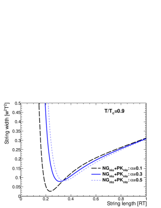
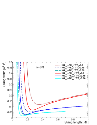
Figure 4: (a) The plot compares the profile of the rigid string for the depicted values of the rigidity parameter $\alpha_{r}$ at next-to-leading-order ($W^{2}=W^{2}_{\rm{NG_{(\ell o)}}}+W^{2}_{\rm{NG_{(n\ell o)}}}+W^{2}_{\rm{Ext_{(\ell o)}}}+W^{2}_{\rm{Ext_{(n\ell o)}}}$) and high temperature $T/T_{c}=0.9$ in the middle plane. (b) The plot shows the profile of the rigid string with respect to the different temperatures. The dashed lines are for the middle plane’s width ($W^{2}=W^{2}_{\rm{NG_{(n\ell o)}}}+W^{2}_{\rm{Ext_{(\ell o)}}}$) at one loop in the rigidity Eqs. (21) and (24); whereas the solid lines are the same as (a) and represent the width at NLO of the rigid string given by Eq.(53).

Compiling all the outcomes of the contribution of the interaction terms to the string width at finite temperature given in Eqs. (43),(51), and (50), the mean-square width is then

$$\scalebox{0.7}{\mbox{$\displaystyle W^{2}_{\rm{Ext_{(n\ell o)}}}=\alpha_{r}\Bigg{[}\left(4(D-2)^{2}-(D-2)\right)\,I^{(2)}_{7}+2(D-2)I^{(2)}_{14}-(D-2)^{2}\,I_{16}^{(2)}\Bigg{]}$}}.$$ (52)

Explicitly, the NLO correction, the second term in Eq. (17), of the smooth string is

(53)

$$\scalebox{0.7}{\mbox{$\displaystyle\times\left(\frac{1}{240}E_{4}\left(\tau\right)+\frac{1}{240}\right)$}}.$$

IV Numerical Discussion

The broadening aspects of the color tube taking into account the rigidity property, can be read off from the LO contribution of the stiff string solution (24). The rigidity impacts on the mean-square width inversely decrease with the square of the length scale $R$. As a result, the influence of stiffness is likely to be more prominent at short and intermediate distances.

The mean-square width $W^{2}$ of the string of the free NG string Eq.(21) in the center plane is displayed versus string length in Fig. 3-(a). In the same figure, we plot the corresponding string width with the received LO geometrical corrections (24) for the depicted values of the rigidity parameter $\alpha_{r}$. One can read off a decrease in the mean-square width for the positive values of the rigidity parameter. The geometrical component in the string action filters out the highly curved configurations and the width profile is finely reduced over a long string length scale. The stiffness, however, has more influence on intermediate and short string length scales, where highly wrinkled surfaces appear more prone to emerge in conventional free effective bosonic theory at high energy.

The mean-square width in Fig. 3-(a) appears to assume negative nonphysical values at finite and positive values of $R$ when $\alpha_{r}=0.3$ or larger. The origin of this effect is readily delineated from the simplest instance when taking the free massless string limit, where the width square at temperature $T=0$ shows logarithmic broadening as Luscher:1980iy

$$W^{2}=\frac{D-2}{4\pi\sigma}\log{\frac{R}{\mu_{0}}}.$$ (54)

The mean-square width returns a negative sign wherever the separation distance between the string end points $R$ is smaller than the UV cutoff $\mu_{0}$. This is a common property among all effective string model solutions Luscher:1980iy ; allais ; Gliozzi:2010zt . The unphysical features at short distance signify the breakdown of the long string approximation over which the effective string theory resides PhysRevLett.67.1681 . The cutoff appears from the standard point-split regularization. The UV-cutoff scale determines $R^{2}_{0}$ of Eq.(21), which is typically regarded as the intrinsic thickness of the string Caselle:2012rp and is intertwined with the long string limit, where $R$ is sufficiently greater than the intrinsic width of the string.

When the rigidity LO correction terms $W^{2}_{{\rm{Ext}}_{(\ell o)}}$ of the PK string (24) are involved, a more stringent form of this effect does occur [Fig.3-(a)]. This also appears to be the case when solutions involving perturbative expansions of boundary terms are considered Aharony:2010cx ; Billo:2012da . It is worth noting that the same observation holds even when the low-energy/long string expansion is truncated at the NLO for the pure NG case, Eq.(38). In Fig. 3-(b), for example, a specific value of the UV-cutoff $\mu_{0}$ parameter is adopted to eliminate nonphysical $W^{2}$ values at the displayed string tensions.

To renormalize to the positive physical values of the width square, the UV cutoff $\mu_{0}$ must subsequently be reset. The renormalization of the string model parameters is not arbitrary and depends on the theory cutoff. For example, the exact dependence of the parameters $\sigma$, $\alpha_{r}$ on the cutoff has been derived in detail in Refs. Nesterenko:1997ku ; PhysRevD.27.2944 ; German:1989vk with the use of two different regularization schemes. In these expressions, the renormalized parameters appear as a function of an UV scale. When comparing effective string theory predictions with lattice gauge theory, setting an energy scale inverse to lattice spacing implies that cutoff and renormalization effects are coupled. In other words, the renormalization effects have an impact on the model’s adjustable parameters via the lattice spacing, which is the characteristic cutoff of the underlying quantum field theory (QFT).

Using the numerical lattice data, the values of the renormalized rigid-string model parameters are determined when fitting the string solution to the lattice, as shown, for example in Refs. Caselle:2014eka ; Brandt:2017yzw for the parameter $\alpha_{r}$. Also, we shall see in the foregoing numerical discussions of the fit of the string model to lattice data, in Table. 1, the comparison between the string models $model_{1}$ and $model_{2}$ of the NG string and $model_{3},model_{4}$, and $model_{5}$ with rigidity corrections. This reveals how the parameter $R_{0}^{2}$ resets its value when including the renormalized $\alpha_{r}$.

In Fig. 4-(a) the mean-square width corresponding to the NLO corrections of the rigidity (53) is plotted at high temperature $T/T_{c}=0.9$. We see that the extrinsic-curvature term Eq.(53) brings on essential corrections on the extracted width of the energy profile at short distances.

A similar plot in Fig. 4-(b) illustrates, however, the perturbative mean-square width with the decrease of the temperature, Eq. (53). The rigidity corrections to the string profile appear to be less compared to the other limit at high temperature/small distances. The curves depicting the mean-square width profile exhibit smaller corrections at low temperatures. This is consistent with the experience that the sharp fluctuations are less probable to occur near the system’s ground state, but rather induced by the thermal effects.

In the limit, $Rm\rightarrow\infty$ with the mass equal to $m=1/\alpha_{r}$, the rigidity term vanishes and the theory approaches the free massless NG string behavior. On the other hand, we identify a divergence at short distances $R$ in the mean-square width of a PK string, as depicted in Fig.4-(b). The PK string model envisaged in the figure is composed from the NG action truncated at NLO, along with the LO and NLO rigidity corrections. The divergence taking place at a relatively short length is not surprising given that the two-loop perturbative expansion converges upon the long string limit.

On the other hand, the extended solutions $W^{2}_{{\rm{Ext}}_{(lo)}}$ and $W^{2}_{{\rm{Ext}}_{(nlo)}}$ of the PK string have been regularized using the $\zeta$ function scheme. Apart from the NG string, examination of the corresponding formulas (24) and (53) demonstrates that they do converge at all separation distances of $R>0$. The NLO terms of the NG action (38), as illustrated in Fig.3-b, are the source of the divergence observed at a comparatively small distance. The divergence arises as a result of terms proportional to the cutoff in Eq.(38).

The long string limit, which sets in the radius of convergence of the low-energy expansion, is intimately related to the intrinsic width of the string and the corresponding cutoff $\mu_{0}$. As previously discussed, applying the LO correction term of the PK string $W^{2}_{{\rm{Ext}}_{(\ell o)}}$ without the corresponding renormalization of the model’s parameter Nesterenko:1997ku ; PhysRevD.27.2944 ; German:1989vk shifts the radius of convergence of the long string limit. It is why the well-behaved region of the width square appears in Fig. 4-(b) to commence at larger $R$. Nevertheless, the plot in Fig. 4-(b) indicates that including the NLO corrections $W^{2}_{{\rm{Ext}}_{(nlo)}}$ has offset this shift to some extent, with the divergence occurring at a smaller length scale.

The NLO rigidity corrections $W^{2}_{{\rm{Ext}}_{(n\ell o)}}$ rapidly scales down the width as one draws closer to the relatively short length of $R$. This is anticipated in the proximity of the radius of convergence of the low-energy perturbative expansion, where higher-order terms ought to provide greater corrections to the mean-square width. Nonetheless, with a reasonable choice of $R$ and $\alpha_{r}$, the precision of the width of the PK string with the NLO rigidity correction terms should be sufficient. For example, if one considers the changes in mean-square width among the curves in Fig. 4-(a) at different values of $\alpha_{r}$, we see that the corrections triggered by the increase in $\alpha_{r}$ exhibit modest variances all the way across the manifested convergence zone.

The effects of the smooth string, though not dominant Caselle:2014eka ; Brandt:2017yzw , are expected to be very relevant to non-Abelian gauge models and in the continuum limit Caselle:2014eka . Nevertheless, the truncation of the perturbative expansion keeping the rigidity corrections at NLO would be favorable when scrutinizing the energy profile on high-resolution lattice data and high temperatures.

In this section, we briefly discuss the rigidity property of QCD flux tube considering the lattice data generated from the simulation setup detailed in Refs. Bakry:2017utr ; Bakry:2018kpn ; Bakry:2020flt . The Monte Carlo data corresponds to pure gluonic configurations of $SU(3)$ Yang-Mills gauge in four dimensions. The space-time dimension of the 4D torus corresponds to $36^{3}\times 8$ at a coupling value of $\beta=6.0$, lattice spacing $a=0.1$ fm and temperature $T/T_{c}=0.9$.

The gauge configurations are generated using the standard Wilson gauge action employing a pseudo-heat bath  FHKP updating to the corresponding three $SU(2)$ subgroup elements  Marinari . Each update step/sweep consists of one heat bath and five microcanonical reflections. The gauge configurations are thermalized following 2000 sweeps.

The multiplication of two Polyakov loops

$$\mathcal{P}_{2Q}(\vec{r}_{1},\vec{r}_{2})=P(\vec{r}_{1})P^{\dagger}(\vec{r}_{2}),$$ (55)

constructs two infinitely heavy static quark-antiquark $Q\bar{Q}$ states on the lattice. After constructing the static meson at a finite temperature, measurement of the Euclidean action density is taken at each point of $SU(3)$ gauge configurations.

Table 1: The returned $\chi^{2}$ from the fits of the theoretical models of both NG and PK string, Eqs. (68)-(72), to the Monte Carlo lattice data of the mean-square width of the Euclidean action density.

	Range	$R\in[0.5,0.7]$ fm			$R\in[0.5,0.8]$ fm			$R\in[0.5,1.2]$ fm
	Model	$\chi^{2}$	$R_{0}^{2}$	$\alpha$	$\chi^{2}$	$R_{0}^{2}$	$\alpha$	$\chi^{2}$	$R_{0}^{2}$	$\alpha$
	$\rm{Model_{1}}$	40.61	2.78(7)	0.0	82.71	2.84(7)	0.0	128.15	2.90 (7)	0.0
	$\rm{Model_{2}}$	9.79	3.2(2)	0.0	22.04	3.3(2)	0.0	31.90	3.4 (4)	0.0
	$\rm{Model_{3}}$	5.35	3.8(2)	0.36(1)	13.82	4.09(2)	0.45(5)	23.00	4.3 (2)	0.51(5)
	$\rm{Model_{4}}$	3.25	3.7(3)	0.1(4)	7.96	4.0(2)	0.13(3)	11.095	4.2(2)	0.15(3)
	$\rm{Model_{5}}$	3.18	4.6(6)	0.12(5)	7.815	5.1(5)	0.16(4)	10.91	5.4(5)	0.18(4)

To characterize the Euclidean action density on the lattice we utilize a plaquette operator defined by

$$\square_{\mu\nu}(\vec{\rho})=1-\frac{1}{3}ReTr\left[U_{\mu}(\vec{\rho})U_{\nu}(\vec{\rho}+\vec{\mu})U_{\mu}^{\dagger}(\vec{\rho}+\vec{\nu})U_{\nu}^{\dagger}(\vec{\rho})\right],$$ (56)

which corresponds to the minimal loop structure on the lattice with the indices $\mu$ and $\nu$ corresponding to Lorentz indices. The plaquette operator can be expanded in a power series Gattringer of the symmetric tensor $F_{\mu\nu}^{c}$ such that

$$\square_{\mu\nu}(\vec{\rho})=1-\frac{1}{3}Re\,Tr\exp\left[\,i\,g\,a^{2}\sum_{c}F^{c}_{\mu\nu}(\vec{\rho})T^{c}\right],$$ (57)

where $g$ is the coupling of Yang-Mills theory, the index $c$ is color indices and $T^{c}$ are the generators of Lie algebra of $SU(3)_{c}$,

$$S(\vec{\rho})=\frac{1}{2}(E^{2}(\vec{\rho})-B^{2}(\vec{\rho})).$$ (58)

The chromoelectric and chromomagnetic components fields are related to the plaquette components at position $\vec{\rho}$ as

$$E^{2}(\vec{\rho})=\sum_{i}E^{2}_{i}(\vec{\rho}) \rightarrow\sum_{i}\square_{0i}(\vec{\rho})$$ (59)

$$B^{2}(\vec{\rho})=\sum_{i}B_{i}^{2}(\vec{\rho}) \rightarrow\sum_{i}\square_{kj}(\vec{\rho}),$$ (60)

where the index $i$ of the magnetic field is the complement of the $j\,k$ plaquette component.

A dimensionless scalar field characterizing the Euclidean action density distribution in the Polyakov vacuum, i.e., in the presence of color sources Bissey:2006bz can be defined as

$$\mathcal{C}(\vec{\rho};\vec{r}_{1},\vec{r}_{2})=\frac{\langle\,\mathcal{P}_{2Q}(\vec{r}_{1},\vec{r}_{2})\,\rangle\,\,\langle S(\vec{\rho})\,\rangle-\langle\mathcal{P}_{2Q}(\vec{r}_{1},\vec{r}_{2})\,S(\vec{\rho})\,\rangle}{\langle\,\mathcal{P}_{2Q}(\vec{r}_{1},\vec{r}_{2})\,\rangle\,\,\langle S(\vec{\rho})\,\rangle},$$ (61)

with the vector $\vec{\rho}$ referring to the spatial position of the energy probe with respect to some origin, and the bracket $\langle...\rangle$ stands for averaging over gauge configurations and lattice symmetries. Other dimensionful definitions of the correlator (61) yield equivalent representation of the width (see, for example Ref. Okiharu:2003vt ).

The above equation is dimensionless. However, the field densities in physical units Bicudo would read

$$\sum_{c}F^{c}_{\mu\nu}F^{c}_{\mu\nu}=\frac{2\beta}{a^{4}}\left[1-\frac{1}{3}Tr(\square_{\mu\nu})\right]+\mathcal{O}(a).$$ (62)

The sum over the color index $c$ ensures the gauge invariance of the square of the field densities.

The measurements are taken on 20 bins separated by 70 sweeps of updates each bin consists of 500 configurations. To avoid artificial reduction of the error bars, each set of 70 update configurations has been included in the same jackknife subensemble, such that the variances are calculated with respect to decorrelated bins.

To eliminate statistical fluctuations with the physical observable left intact, only 20 sweeps of UV filtering of stout-link smearing Morningstar:2003gk have been applied on each considered gauge configuration. We make use of the symmetry of the 4D torus, that is, the measurements that are taken at a fixed color source’s separations $R$ are repeated and averaged. The characterization (61) yields $0<C<1$ with $C\rightarrow 0$ away from the quarks by virtue of the cluster decomposition of the operators.

To estimate the mean-square width of the gluonic action density along each transverse plane to the quark-antiquark axis by taking into consideration the axial cylindrical symmetry of the tube, we choose a double Gaussian function of amplitude $A$ and fit parameters $\sigma_{1},\sigma_{2}$ and $\kappa$, such that

$$G(r,\theta;z)=A(e^{-r^{2}/\sigma_{1}^{2}}+e^{-r^{2}/\sigma_{2}^{2}})+\kappa.$$ (63)

A measurement of the width of the Euclidean action density may be taken by fitting the density distribution $\mathcal{C}(\vec{\rho};z)$ to Eq.(63) through each transverse plane to the cylinder’s axis $z$ to Eq.(63), with $r^{2}=x^{2}+y^{2}$ in each selected transverse plane $\vec{\rho}(r,\theta;z)$, which returns acceptable values of $\chi^{2}$ at the intermediate and long distances Bakry:2020ebo .

There is another justification behind the selection of this ansatz other than the good parametrization behavior over the targeted distance scale Bakry:2020ebo . The reason comes from the observation of a large difference in the value of the returned fit parameters satisfying the width $\sigma_{1}\gg\sigma_{2}$. That is, when parametrizing the transverse profile with this particular form, the usual Gaussian function receives corrections from a narrower Gaussian with the same amplitude. The overlap of a two Gaussian of the same amplitude and different width reweighs the fit function at the center of the profile with respect to the tail of the bell-shaped region.

The form is inspired by the fit function as shown in Ref. Bicudo where a classical flux-tube profile is convoluted with a Gaussian distribution relevant to the quantum oscillations. The form in Ref. Gliozzi:2010zv also corrects the tube center near the $Q\bar{Q}$ axis and asymptotically appears to reweigh the tail region. It should be noted that, with the use of these fit ansatz introduced in the aforementioned reference, we obtained good fits at small separation distances; however, we received large error bars at large distances. For convenience, we have recoursed to the two Gaussian forms, which describe one way to mimic the same function.

The second moment of the action density distribution with respect to the cylinder’s axis $z$ joining the two quarks is

$$W^{2}(z_{i})=\quad\frac{\int\,dr\,r^{3}\,G(r,\theta;z_{i})}{\int\,dr\,r\>G(r,\theta;z_{i})},$$ (64)

which defines the $i$-th data entry of the mean-square width of the tube at the plane $z_{i}$ on the lattice.

The measurements of the mean-square width of the Euclidean action density have been achieved with a good signal-to-noise ratio and are obtained by employing only 20 sweeps of stout-link smearing Bakry:2017utr ; Bakry:2018kpn ; Bakry:2020ebo . The small number of stout-link smearing sweeps should increase the accuracy of the measurement and keep the relevant physics intact, for the targeted color separation distance scale Bakry:2014ina . All the most recent calculated data relevant to the Euclidean action density with the fit analysis and width measurements have been included in Refs. Bakry:2017utr ; Bakry:2018kpn ; Bakry:2020ebo in detail.

In general, renormalization effects Peter impact lattice measurements via lattice spacing, which establishes a natural cutoff for the corresponding QFT. Setting an energy scale inverse to lattice spacing entails that cutoff and renormalization effects are entangled; any change in the scale is also a change in the cutoff. When measuring the width, a change in the cutoff offsets the width by an overall constant. This induction is based on the observation of an identical impact on the width Bakry:2010sp due to the application of a different number of cooling sweeps, which effectively increases lattice spacing or changes the UV scale. In the present setup, we study the behavior of the quantum broadening of the width, which would be unaffected by the same overall shifts at a given $R$.

Another subtlety concerning the width measurement comes from the issue of possible cross-correlations among the correlators at various distances. The computations of the field densities involve a three-point correlation function consisting of two Polyakov loops in opposite directions and the flux-tube operator, Eq. (61). In this setup, when the size of the flux probe operator is substantially large, cross-correlations among measurements at a different distances could be prone to occur on the same gauge configuration. Large size/extended operators involve nested loops with different sizes, which is a well-known strategy in LGTs to minimize the discretization errors owing to the lattice spacing. In the present calculations, we applied the simplest “one-loop field strength tensor operator”, which is proportional to one plaquette and is the minimal-sized loop structure on hypercubic lattices, to compute chromoelectric and chromomagnetic field densities Eqs.(60) and (62). For the same reason, we avoided using algorithms utilizing extended operators in the stout-link smearing besides the small number of smearing sweeps to minimize blurring (Brownian motionTakahashi:2002bw ) of gauge links.

We may add to the above one more point that comes from the lattice setup where the Monte Carlo simulations with the standard Wilson gauge action ensure locality Luscher:2001up . In addition, the heat bath combined with overrelaxation / microcanonical steps would assist to diverge the autocorrelation time QCD-TARO:1992iba .

As a consistency check of cross-correlation between adjacent Polyakov loop correlators, we calculate the local string tension and convert to lattice spacing $a$ in Fermi units using the transfer matrix interpretation Luscher:2001up , such that

$$\alpha(\Lambda)\,\exp(-\sigma RL_{T})=\langle P(0)P^{\dagger}(R)\rangle$$ (65)

$$\sigma a^{2}=-\frac{1}{L_{T}}\log\left(\frac{\langle P(0)P^{\dagger}(R+1)\rangle}{\langle P(0)P^{\dagger}(R)\rangle}\right)$$ (66)

The lattice spacing in Fermi units is then

$$a=\frac{0.1973\rm{GeV\,fm}}{\sqrt{0.440}\rm{GeV}}\left[-\frac{1}{L_{T}}\log\left(\frac{\langle P(0)P^{\dagger}(R+1)\rangle}{\langle P(0)P^{\dagger}(R)\rangle}\right)\right]^{\frac{1}{2}}$$ (67)

on each gauge configuration. The above expectation values are calculated as average on all lattice points utilizing the lattice space-time symmetries to improve the statistics in a gauge-independent manner. The purpose of these measurements is to test if we could extract the correct value of the lattice spacing $a\simeq 0.098$ from two Polyakov loops correlators at a different distance. We report the correct value of the lattice spacing which indicates the minor effect of cross-correlations among adjacent Polyakov loop correlators at various distances.

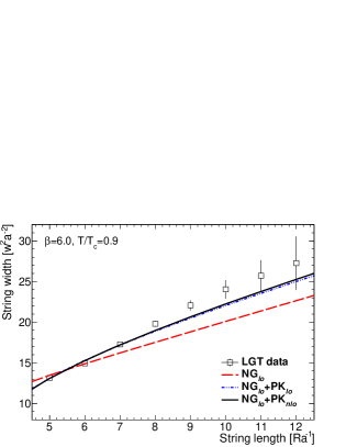
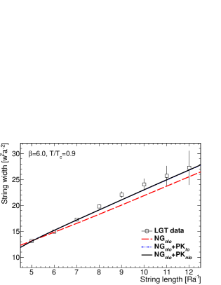
Figure 5: The mean-square width of the string $W^{2}(R/2)$ versus $Q\bar{Q}$ separations measured in the middle plane $R/2$ at $T/T_{c}=0.9$.(a) The fits of the LO width square of NG string, Eq. (21) and combination of rigidity contributions given by PK string models Eqs. (70)-(72). (b) The fits of the NLO width of NG string, Eq. (38), and combination of rigidity contributions given by PK string models Eqs. (70)-(72). The Monte Carlo lattice data of the square width of the Euclidean action density width are shown with boxes. The lattice data have been fitted in the interval $R\in[0.5,0.7]$ fm.

The numerical values Bakry:2017utr ; Bakry:2018kpn ; Bakry:2020ebo of the mean-square width indicate a broadening in mean-square width of the string at all transverse planes $z_{i}$ as the color sources are pulled apart a distance $R_{i}$. The maximum color source separation distance has been taken up to $R=1.2$ fm, which is one-third the total spatial extent of the lattice 3.6 fm to avoid cross-correlations through the toroidal lattice owing to the periodic boundary condition. At the central transverse plane $z_{i}=R/2$, the pattern of the width broadening (64) can be compared to prescribed width models that combine an assortment of potentially interesting quantum string corrections.

In addition to the pure NG string models at two orders,

$$W^{2}_{model_{1}}=W^{2}_{\rm{NG_{(\ell o)}}},$$ (68)

$$W^{2}_{model_{2}}=W^{2}_{\rm{NG_{(\ell o)}}}+W^{2}_{\rm{NG_{(n\ell o)}}},$$ (69)

which are given in accordance with Eqs.(21) and (38), respectively. The following three models define selected combinations with the rigidity corrections:

$$W^{2}_{model_{3}}=W^{2}_{\rm{NG_{(\ell o)}}}+W^{2}_{\rm{Ext_{(\ell o)}}},$$ (70)

$$W^{2}_{model_{4}}=W^{2}_{\rm{NG_{(\ell o)}}}+W^{2}_{\rm{NG_{(n\ell o)}}}+W^{2}_{\rm{Ext_{(\ell o)}}},$$ (71)

$$W^{2}_{model_{5}}=W^{2}_{\rm{NG_{(\ell o)}}}+W^{2}_{\rm{NG_{(n\ell o)}}}+W^{2}_{\rm{Ext_{(\ell o)}}}+W^{2}_{\rm{Ext_{(n\ell o)}}},$$ (72)

which are provided by Eqs.(21), (38), (24) and (53).

The fits are obtained by optimizing the sets of the parameter space ${R_{0},\alpha}$ in the above-mentioned models such that the least square residuals

$$\chi^{2}(R_{0},\alpha)=\frac{\sum_{i}(W^{2}_{i}(R_{i}/2)-W^{2}_{model}(R_{i}/2;R_{0},\alpha))^{2}}{\sum_{i}e_{i}^{2}(R_{i}/2)},$$ (73)

are minimized. In the above equation (73), $e_{i}^{2}(R_{i}/2)$ is the square of the error in the measured mean-square width $W^{2}_{i}(R_{i}/2)$ from the lattice simulation (64).

Here, the analysis of the fit behavior of the mean-square width data is discussed keeping the string tension fixed to the standard value Schilling93 of $\sqrt{\sigma}=440$ MeV. Our interest is to divulge the rigidity parametrization behavior at each order of the perturbative expansion of the PK string with respect to numerical data. We consider the lattice data of the mean-square width of the QCD flux tube at the perpendicular plane in the middle $R/2$ between the color sources Bakry:2017utr ; Bakry:2018kpn ; Bakry:2020ebo .

The resultant minimum $\chi^{2}$ and the corresponding fit parameters $\alpha$ and $R_{0}^{2}$ from the fits to the lattice data Eq.(73) are collected in Table. 1. The first column of the table highlights the five string models defined by Eqs.(68) - (72). That is, in the first two rows, the fit parameter $R_{0}^{2}$ (related to the UV cutoff) returned from the fit to the width at both the LO and the NLO mean-square width of the NG string Eq.(68) and (69), respectively. However, in the next entries the table includes the values of both $R_{0}^{2}$ and the rigidity $\alpha_{r}$ parameters returned from the fits to the mean-square width for selected models of the PK string, Eqs.(70)-(72).

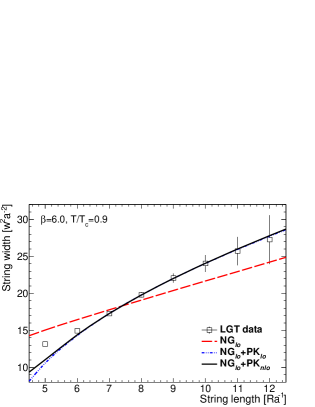
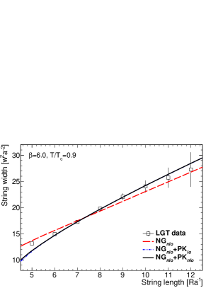
Figure 6: Same as Fig. 5, the mean-square width of the string $W^{2}(R/2)$ versus $Q\bar{Q}$ separations measured at the middle plane $R/2$ at $T/T_{c}=0.9$, however, the fit range involves larger source separation $R\in[0.7,1.2]$ fm. (a) The fits of the LO width square of NG string, Eq. (21) and combination of rigidity contributions given by PK string models Eqs. (70)-(72). (b) The fits of the NLO width of NG string, Eq. (38), and combination of rigidity contributions given by PK string models Eqs. (70)-(72).

The returned $\chi^{2}$ values, in Table.1, imply that the fits are better with respect to the pure NG string (69) at NLO than with the LO approximation (68). Nonetheless, the NLO approximation does not produce an optimal match with the numerical data until large source separations $R\geq 0.8$ fm.

Further examination of $\chi^{2}$ values from the fit of $W^{2}_{model_{3}}$ of the PK string (70) reveals an improvement over fits of $W^{2}_{model_{1}}$ pertinent to the free-string model (68). This PK string model, in which the LO rigidity corrections appear to play a similar role to the string self-interaction, yields acceptable $\chi^{2}$ values over a fit interval of $R\in[0.6,1.2]$ fm.

Despite the reduction in $\chi^{2}$ values when considering either the PK string’s rigidity or the NG string’s self-interaction, we find that combining both corrections yields better values of $\chi^{2}_{\rm{d.o.f.}}=10.91/6$ over the entire source separation interval $R\in[0.5,1.2]$ fm.

When the fit behavior of the LO and the NLO corrections of smooth PK string models [Eq.(71) and (72)] is opposed, the values of the returned $\chi^{2}$ are found to differ slightly. The corrections acquired from the NLO stiffness terms are relatively minor and within the measurement uncertainties. The projected improvements from these NLO terms can be significant if smaller length scales, finer lattices, or alternate gauge models are considered, which are beyond the scope of this study. Nonetheless, the fit findings show that the NLO perturbative modifications are consistent with the lattice data at typical values of the rigidity parameter $\alpha_{r}$.

Figs.5 and 6 reflect the above discussed points, including the $\chi^{2}$ values in Table.1, in particular the improvement in the fit with respect to the rigid PK string compared to that obtained merely on the basis of the pure NG string. The plots in Figs.5 and 6 are for fits to Eqs.(21) and (38) in addition to Eqs.(70)-(72). The fits are over a subset of the intermediate source separation region $R\in[0.5,0.7]$ fm Fig.5. The Fig.6 renders curves from the fits over the subset $R\in[0.7,1.2]$ fm at the end.

The graphs in Figs.5 and 6 show the mean-square width as calculated using the theoretical models of Eqs.(68)-(72). Fig.5 depicts fitted curves over source separation $R\in[0.5,0.7]$, whereas Fig. 6 displays the fitted width square over $R\in[0.7,1.2]$. Both figures, as well as the $\chi^{2}$ values in Table 1 reflect the arguments highlighted above, specifically the improvement in fit with respect to the stiff PK string compared to that produced purely on the basis of the NG string.

For source separation range $R\in[0.5,0.7]$ fm, the rendering in Fig.5 of the fitted width of the pure NG string at either order exhibits significant deviations from the lattice data compared to the fits in Fig.6 over the fit interval $R\in[0.7,1.2]$ fm. The plots in Fig.5 suggest the incompetence of the pure NG string as a physical description integrating the subtle features of the QCD flux tubes. However, for both fit intervals, the improvements with respect to the rigid PK string models [Eqs.(70)-(72)] are clearly evident in Figs.5 and 6.

In regard to the stability of the fits, we find the values of $\alpha_{r}$ to be equal (within the uncertainties) and stable for all fit intervals commencing from $R_{min}=0.5$ fm ($R\in[R_{min},R_{max}]$) up to $R_{max}=1.2$ fm. Moreover, we report the same value of $\alpha_{r}$ for the fit intervals commencing from $R_{min}=0.4$ fm as well Bakry:2020ebo .

It should be noted that the small values of the returned $\chi^{2}_{\rm{d.o.f.}}<1$, for the fit of rigid models $model_{3}-model_{5}$ on the other intervals such as $R\in[0.7,1.2]$, are indicating the growing width of the error bars at a large distance. However, stability and consistency with the returned values in the above can be checked by substituting the returned values of $\alpha_{r}$ on any of the former intervals within the latter, which produces fits with acceptable values of $\chi^{2}_{\rm{d.o.f.}}$ and thereof proves the stability of the fits. In addition, we find the returned value of $\alpha_{r}$ from the fits of the highly accurate $Q\bar{Q}$ potential data to rigid-string model on these intervals reproduces the values $\alpha_{r}$ within the uncertainties Bakry:2020flt .

The properties of the energy profile of the smooth QCD string ought to be discerned in the light of the counterpart IR observable, namely, the string tension and the $Q\bar{Q}$ potential. Our up-to-date lattice simulation and fit analysis of the static $Q\bar{Q}$ data have been reported in detail in Ref. Bakry:2020flt (see also Refs. Bakry:2017utr ; Bakry:2018kpn ; Bakry:2020ebo ).

The pure NG string at the NLO does not provide a precise match to the numerical data of the static $Q\bar{Q}$ potential either Bakry:2020flt . Fits to the PK string at leading order, on the other hand, return a stable minimum in the $\chi^{2}$ for a rigidity factor of roughly $\alpha_{r}\approx 0.3(2)$ on the interval $R\in[0.6,1.1]$ fm (without boundary corrections) Bakry:2020flt . Remarkably, by the inclusion of the rigidity terms in $Q\bar{Q}$ string potential, the accurate value of the string tension of $\sigma a^{2}=0.044$  Koma:2017hcm is reproduced when taken as a free fit parameter. We plug both values of fit parameters $\sigma$ and $\alpha_{r}$ in Eq.(70) for the fit to the mean-square width of flux tube as a consistency check, and we attain good $\chi^{2}$ values in the fit range $R\in[0.6,1.2]$ fm.

The close fit produced from the two probes of the confining string, namely, the energy profile and the $Q\bar{Q}$ potential, possibly supports the faithfulness of the physics of the smooth QCD string rather than being a mere artifact of the model’s extended parametric space.

V Summary and Conclusion

In summary, we have considered the geometrical (PK) string proposed by Polyakov POLYAKOV19 and Kleinert Kleinert:1986bk , in which the surface representation in the string action depends on the area as well as the geometrical configuration of the embedded world sheet. This is embodied in the effective bosonic string action by introducing terms proportional to the extrinsic-curvature as a next-order operator after the NG action POLYAKOV19 ; Kleinert:1986bk . The curvature term with a positive-valued rigidity parameter favors the smooth string’s world sheet configurations over the sharply creased surfaces.

In this work, we have derived the width of the energy profile of PK rigid strings in $D$ dimension at both low and high temperatures. The perturbative arguments regarding string’s rigidity have been implemented as an effective low-energy parameter expansion around the encompassed NG string action. That is, the perturbative expansion of the extrinsic-curvature term is taken around the free NG string action.

The technique of the $\zeta$ function is incorporated in the regularization of the divergent sums appearing in the corresponding expectation values of the mean-square width of the string. The resultant Green’s function integrals have been evaluated with an open-string propagator on a cylinder, i.e., the Dirichlet boundary condition. Our main results are given by Eq.(24) for the width corrections at the LO level and Eq.(53) for the NLO corrections, which lay out a general expression valid at any temperature and dimension.

The LO rigid-string correction to the mean-square width Eq.(24) indicates an inverse decrease with the square of the length scale $R$. As expected, this entails rigidity effects that are outstanding near the intermediate and short string length scale. The next-to-leading expression of rigid-string correction Eq.(53), introduces delicate corrections of the mean-square width over short distances, which would extend the applicability of the derived formula.

We have examined the width corrections induced by the smooth PK string with respect to the numerical lattice data for a high temperature close to the deconfinement point $T/T_{c}=0.9$. We consider lattice data corresponding to the Monte Carlo simulations of the flux tube profile in the middle plane in pure $SU(3)$ Yang-Mills theory in four dimensions Bakry:2017utr ; Bakry:2018kpn ; Bakry:2020ebo . The fits of the mean-square width considering the rigidity and self-interaction corrections are in a good match with the lattice Monte Carlo data of QCD flux tube at both intermediate and large color source separation distances.

Nevertheless, it remains demanding to layout the width profile taking into account the Lorentz-invariant boundary action Billo:2012da ; Bakry , exploring the full effective string actions in the numerical simulation of $SU(3)$ Yang-Mills theory Bakry:2020ebo and other gauge models. The energy  Bicudo:2018jbb profile of the excited meson is a very relevant system to implement such a program as well. In addition to that, it would be interesting to consider other boundary conditions involving open strings; such as the mixed Dirichlet-Neumann boundary condition, which generalizes the discussed theoretical considerations to the baryonic configurations Jahn2004700 ; deForcrand:2005vv ; Pfeuffer ; Bakry:2016aod ; Bakry:2014gea . This is the target of our next reports.

Appendix A Functions and Identities

The following outlines functions and identities WhittakerWatson ; abramowitz ; Erdelyi that will be used along with the calculations of perturbative corrections to the mean-square width:

• The Dedekind $\eta$ function over the complex plane is defined as

  $$\eta(\tau) =q^{\frac{1}{24}}\prod_{k=1}^{\infty}\left(1-q^{k}\right)$$ (74)

  $$=e^{\frac{i\pi\tau}{12}}\prod_{k=1}^{\infty}\left(1-e^{2i\pi k\tau}\right),$$

  with $q=e^{2i\pi\tau}$ and $\tau=\frac{iL_{T}}{2R}$. The identity

  $$\sum_{j=1}^{\infty}\log\left(1-q^{j}\right)=\log\left(q^{-\frac{1}{24}}\eta(\tau)\right),$$ (75)

  also follows from the above definition.

• The Eisenstein series over the complex plane is defined as

  $$E_{2k}(\tau)=1+(-1)^{k}\frac{4k}{B_{k}}\sum_{n=1}^{\infty}\frac{n^{2k-1}}{1-q^{n}},$$ (76)

  where $B_{k}$ are Bernoulli numbers defined as

  $$\mathbf{\zeta}(2k)=\frac{B_{k}(2\pi)^{2k}}{2k!},~{}~{}~{}~{}~{}~{}~{}~{}~{}\mathbf{\zeta}(1-2k)=(-1)^{k}\frac{B_{k}}{2k!}.$$ (77)

  for even and odd numbers respectively.

  In particular, $E_{2}$ and $E_{4}$ are given by

  $$E_{2}(\tau)= 1-24\sum_{n=1}^{\infty}\frac{n}{1-q^{n}},$$ (78)

  $$E_{4}(\tau)= 1+240\sum_{n=1}^{\infty}\frac{n^{3}}{1-q^{n}}.$$ (79)

  The modular transform $\tau\rightarrow\frac{-1}{\tau}$ of the Dedekind $\eta$ function and the Eisenstein series $E_{2k}$ is given by

  $$\eta({\tau}) =\frac{1}{\sqrt{i\tau}}\eta\left(\frac{-1}{\tau}\right),$$ (80)

  $$E_{2}(\tau) =\frac{1}{\tau^{2}}E_{2}\left(\frac{-1}{\tau}\right)-\frac{1}{6i\pi\tau},$$ (81)

  respectively.

• Identity(I):
  The sum $\sum_{n}\frac{n\left(q^{n}+1\right)}{q^{n}-1}$ can be expressed in the form of the Eisenstein series

  $$\sum_{n}\frac{n\left(q^{n}+1\right)}{q^{n}-1} =\sum_{n}\frac{n}{q^{n}-1}-\sum_{n}\frac{nq^{n}}{1-q^{n}}$$ (82)

  $$=\sum_{n}\frac{n}{q^{n}-1}-\sum_{n}\frac{nq^{n}}{1-q^{n}}$$

  $$=\sum_{n}\frac{n}{q^{n}-1}-\frac{1}{24}(1-E_{2}(\tau))$$

  $$=\sum_{n}\frac{n\left(q^{n}-q^{n}+1\right)}{q^{n}-1}-\frac{1}{24}(1-E_{2}(\tau))$$

  $$=-\frac{2}{24}(1-E_{2}(\tau))-\sum_{n}n$$

  $$=\frac{1}{12}-\frac{2}{24}(1-E_{2}(\tau))$$

  $$=\frac{1}{12}E_{2}(\tau).$$

• Identity(II) The product representation of the Jacobi elliptic theta function of the first kind $\vartheta_{1}(z,q)$ is defined as

• Identity(III) The logarithmic derivatives of $\vartheta_{1}(z,q)$ can be expressed as a series sum of hyperbolic functions as

  $$\sum_{k=-\infty}^{\infty}\coth(\pi k\lambda+z)=i\frac{\vartheta_{1}^{\prime}\left(iz,e^{-\pi\lambda}\right)}{\vartheta_{1}\left(iz,e^{-\pi\lambda}\right)}.$$ (84)

• Identity(IV) The modular $\pi\tau$ increment in the argument of the $\vartheta_{1}$ function has the property

  $$\vartheta_{1}(\pi\tau+z,q)=-\frac{e^{-2iz}}{q}\vartheta_{1}(z,q).$$ (85)

  The generic formula for $m\in\mathbf{Z}$ for the modular increment of $z$,

  $$\vartheta_{1}(z+m\pi\tau,q)=\frac{(-1)^{m}}{q^{m}}\vartheta_{1}(z,q)e^{-i(\pi(m-1)m\tau+2mz)}.\\$$ (86)

  The modular increase of the logarithmic derivative can be deduced from properties of the $\vartheta_{1}$ function; for $m=-1$ we obtain

  $$\frac{\vartheta_{1}^{\prime}(z-\pi\tau,q)}{\vartheta_{1}(z-\pi\tau,q)}=\frac{\vartheta_{1}^{\prime}(z,q)}{\vartheta_{1}(z,q)}-2i,$$ (87)

  and

  $$\frac{\vartheta_{1}^{\prime\prime}(z-\pi\tau,q)}{\vartheta_{1}(z-\pi\tau,q)}=\frac{\vartheta^{\prime\prime}\left(1,z,q\right)}{\vartheta_{1}\left(z,q\right)}+\frac{4i\vartheta_{1}^{\prime}\left(z,q\right)}{\vartheta_{1}\left(z,q\right)}-4.$$ (88)

• Identity(V) The square of the logarithmic derivative Zhao ; SHEN1993299 of the theta function $\vartheta_{1}$ is given by

  $$\left(\frac{\vartheta_{1}^{\prime}(z,q)}{\vartheta_{1}(z,q)}\right)^{2}=\frac{\vartheta_{1}^{\prime\prime}(z,q)}{\vartheta_{1}(z,q)}-\left(\frac{\vartheta_{1}^{\prime}(z,q)}{\vartheta_{1}(z,q)}\right)^{\prime}.$$ (89)

• Identity(VI):

  $$\sum_{k=1}^{\infty}\frac{k^{3}}{1-q^{k}} =\frac{k^{3}\left(q^{k}-q^{k}+1\right)}{1-q^{k}}$$

  $$=\sum_{k=1}^{\infty}\frac{k^{3}q^{k}}{1-q^{k}}+\sum_{k=1}^{\infty}k^{3}$$

  $$=\frac{1}{240}(E_{4}(\tau)-1)+\mathbf{\zeta}(-3).$$ (90)

• Identity(VII) The following quotient of the second derivative of the elliptic $\theta_{1}$ function has the series representation Zhao ; SHEN1993299 given by

  $$\scalebox{0.7}{\mbox{$\displaystyle\frac{\vartheta_{1}^{\prime\prime}\left(z,e^{-\frac{L\pi}{2R}}\right)}{\vartheta_{1}\left(z,e^{-\frac{L\pi}{2R}}\right)}=16\sum_{n=1}^{\infty}\frac{e^{-\frac{(\pi L)n}{2R}}\cos(2nz)}{\left(1-e^{-\frac{(\pi L)n}{2R}}\right)^{2}}+8\sum_{n=1}^{\infty}\frac{ne^{-\frac{(\pi L)n}{2R}}}{1-e^{-\frac{(\pi L)n}{2R}}}-1$}}.$$ (91)

  .

• Identity(VIII) The Jacobi elliptic theta function $\vartheta_{4}(z,q)$ is defined as an infinite product such that

  $$\scalebox{0.9}{\mbox{$\displaystyle\vartheta_{4}(z,q)=\prod_{k=1}^{\infty}\left(1-q^{2k}\right)\left(-2q^{2k-1}\cos(2z)+q^{4k-2}+1\right)$}}.$$ (92)

• Identity(IX) The modular increment of the argument of the Jacobi elliptic $\vartheta_{4}$ is equivalent to

• Identity(X) The products that appear in Eq. (149) as a result of the algebraic manipulations of the sums are related to the elliptic $\theta_{4}$. For instance, the following shows explicitly this relation for the product:
  

  $$\mathcal{P}_{1} =-\prod_{k=1}^{\infty}\left(1-e^{-\frac{\pi kL_{T}}{2R}+\frac{\pi L_{T}}{R}}\right)\left(1-e^{-\frac{\pi kL_{T}}{2R}-\frac{\pi L_{T}}{2R}}\right)$$

  $$\scalebox{0.85}{\mbox{$\displaystyle=\frac{1}{G_{1}}\vartheta_{4}\left(\frac{i(3L_{T}\pi)}{8R},e^{-\frac{L_{T}\pi}{4R}}\right)$}};$$

  with $G_{1}=\prod_{k=1}^{\infty}\left(1-e^{-\frac{\pi kL_{T}}{2R}}\right)$

• Identity(XI):
  The logarithmic series

  (95)

  $$\scalebox{0.85}{\mbox{$\displaystyle=\sum_{j=1}^{\infty}\log\left(1-q^{j}\right)-\lim_{\epsilon\to 0}\,\frac{1}{2}(\mathbf{\zeta}(1-\epsilon)+\mathbf{\zeta}(\epsilon+1))$}},$$

  owing to the harmonic series defined as,

  $$\zeta(k)=\sum_{n=1}^{\infty}\frac{1}{n^{k}},$$ (96)

  diverges at $k=1$. The principle value of $\mathbf{\zeta}(1)$ is $\gamma$, where $\gamma=0.5772$ is the Euler-Mascheroni constant.
  

• Zeta Regularization
  In the following, we quote the partition of some basic properties of the zeta-regularized products Yoshimoto2002 . Let us consider the convergence index, which is the least integer $h$ such that the series for $Z[h+1]$ converges absolutely.
  One-partition property.
  Let $\{\varphi^{1}\}_{k}$ and $\{\varphi^{2}\}_{k}$ be $\mathbf{\zeta}$- and let regularizable sequences $\{\varphi\}_{k}=\{\varphi^{1}\}_{k}\cup\{\varphi^{2}\}_{k}$ disjoint union then

  $$\prod_{k}\varphi_{k}=\prod_{k}\{\varphi^{1}\}_{k}\prod_{k}\{\varphi^{2}\}_{k}.$$ (97)

  Two-splitting property.
  If $\{\varphi_{k}\}$ is zeta-regularizable and $\prod_{k}a_{k}$ is convergent absolutely, then

  $$\prod_{k}a_{k}\varphi_{k}=\prod_{k}a_{k}\prod_{k}\varphi_{k}.$$ (98)

Appendix B The free-string propagator and width on cylinder

The Green’s correlator can be expressed in terms of Jacobi theta functions

$$G(\mathbf{\zeta;\zeta^{\prime}}) =\frac{1}{\pi\sigma}\sum_{n=1}^{\infty}\frac{1}{n\left(1-q^{n}\right)}\sin\left(\frac{\pi n\zeta}{R}\right)\sin\left(\frac{\pi n\zeta^{\prime}}{R}\right)$$

$$~{}~{}~{}~{}~{}~{}~{}~{}~{}~{}~{}~{}~{}~{}\scalebox{0.9}{\mbox{$\displaystyle\times\left(q^{n}e^{\frac{\pi n(\zeta_{0}-\zeta^{{}^{\prime}}_{0})}{R}}+e^{-\frac{\pi n(\zeta_{0}-\zeta^{{}^{\prime}}_{0})}{R}}\right)$}},$$

where $q=e^{-\pi\frac{L_{T}}{R}}$ is the complementary nome.

Let us define the following auxiliary identities:

$$\kappa_{1} =(\zeta_{0}^{{}^{\prime}}-\zeta_{0}-i\zeta-i\zeta^{\prime}),$$ (100)

$$\kappa_{2} =(\zeta_{0}^{{}^{\prime}}-\zeta_{0}+i\zeta-i\zeta^{\prime}),$$ (101)

$$\kappa_{3} =(\zeta_{0}^{{}^{\prime}}-\zeta_{0}-i\zeta+i\zeta^{\prime}),$$ (102)

$$\kappa_{4} =(\zeta_{0}^{{}^{\prime}}-\zeta_{0}+i\zeta+i\zeta^{\prime}).$$ (103)

With these identities, the Green’s function from Eq.(B) can be recast as

$$G(\kappa)=\frac{1}{4\pi\sigma}\sum_{n=1}^{\infty}\frac{1}{n\left(1-q^{n}\right)}$$ (104)

$$=\frac{1}{4\pi\sigma}\sum_{n=1}^{\infty}\frac{1}{n\left(1-q^{n}\right)}$$

$$~{}~{}~{}~{}~{}~{}~{}~{}~{}~{}~{}~{}~{}~{}~{}~{}~{}~{}~{}~{}~{}~{}~{}~{}~{}~{}~{}~{}~{}~{}~{}~{}~{}~{}~{}~{}~{}~{}~{}\scalebox{0.9}{\mbox{$\displaystyle-\left(q^{n}e^{-\frac{\pi n\kappa_{4}}{R}}+e^{\frac{\pi n\kappa_{4}}{R}}\right)\Bigg{]}$}}.$$

Considering the general term in the sum

$$S(\kappa) =\sum_{n=1}^{\infty}\frac{1}{n\left(1-q^{n}\right)}\left(q^{n}e^{-\frac{(\pi n)\kappa}{R}}+e^{\frac{(\pi n)\kappa}{R}}\right)$$ (105)

$$=\sum_{n=1}^{\infty}\left(\sum_{k=1}^{\infty}\frac{q^{kn}e^{-\frac{(\pi n)\kappa}{R}}}{n}+\sum_{k=0}^{\infty}\frac{q^{kn}e^{\frac{(\pi n)\kappa}{R}}}{n}\right)$$

$$=-\sum_{k=0}^{\infty}\log\left(1-q^{k}e^{\frac{\pi\kappa}{R}}\right)-\sum_{k=1}^{\infty}\log\left(1-q^{k}e^{-\frac{\pi\kappa}{R}}\right)$$

$$=-\log\left[\prod_{k=0}^{\infty}\left(1-q^{k}e^{\frac{\pi\kappa}{R}}\right)\prod_{k=1}^{\infty}\left(1-q^{k}e^{-\frac{\pi\kappa}{R}}\right)\right]$$

$$=-\log\left[\prod_{k=1}^{\infty}\left(1-q^{k-1}e^{\frac{\pi\kappa}{R}}\right)\left(1-q^{k}e^{-\frac{\pi\kappa}{R}}\right)\right]$$

$$=\log\left[\prod_{k=1}^{\infty}\left(1-q^{k}\right)\right]$$

$$-\log\left[\prod_{k=1}^{\infty}\left(1-q^{k}\right)\left(1-q^{k-1}e^{\frac{\pi\kappa}{R}}\right)\left(1-q^{k}e^{-\frac{\pi\kappa}{R}}\right)\right].$$

Using the results for the general term in $G(\kappa_{i})$ and with some algebraic manipulations, the propagator in Eq.(104) becomes

$$G(\kappa)=\frac{1}{4\pi\sigma}\log\Bigg{[}\frac{A_{\kappa_{1}}A_{\kappa_{4}}}{A_{\kappa_{2}}A_{\kappa_{3}}}\Bigg{]},$$ (106)

where

$$A_{\kappa_{i}}=\prod_{n=1}^{\infty}\left(1-q^{n}\right)\left(1-q^{n-1}e^{\frac{\pi\kappa_{i}}{R}}\right)\left(1-q^{n}e^{-\frac{\pi\kappa_{i}}{R}}\right),$$ (107)

$$i=1,...,4.$$

In terms of Jacobi theta functions, the propagator in Eq.(106) reads

(108)

$$\scalebox{0.75}{\mbox{$\displaystyle=\frac{1}{4\pi\sigma}\log\Bigg{[}\frac{\vartheta_{4}\left(-\frac{(i\pi)\kappa_{1}}{2R}-\frac{i\pi L_{T}}{4R},e^{-\frac{\pi L_{T}}{2R}}\right)\vartheta_{4}\left(-\frac{(i\pi)\kappa_{4}}{2R}-\frac{i\pi L_{T}}{4R},e^{-\frac{\pi L_{T}}{2R}}\right)}{\vartheta_{4}\left(-\frac{(i\pi)\kappa_{2}}{2R}-\frac{i\pi L_{T}}{4R},e^{-\frac{\pi L}{2R}}\right)\vartheta_{4}\left(-\frac{(i\pi)\kappa_{3}}{2R}-\frac{i\pi L_{T}}{4R},e^{-\frac{\pi L_{T}}{2R}}\right)}\Bigg{]}$}}.$$

Using the following transformation $\xi_{i}=\frac{-i\pi}{2}\left(\frac{\kappa_{i}}{R}+\frac{L_{T}}{2R}\right)$ the propagator can be recast into the following closed form:

$$G(\xi)=\frac{1}{4\pi\sigma}\log\left[\frac{\theta_{4}\left(\xi_{1},\sqrt{q}\right)\theta_{4}\left(\xi_{4},\sqrt{q}\right)}{\theta_{4}\left(\xi_{2},\sqrt{q}\right)\theta_{4}\left(\xi_{3},\sqrt{q}\right)}\right].$$ (109)

Appendix C Contribution of LO term of extrinsic curvature

The next term in Eq.(14) representing the LO perturbation due to the instantaneous string in terms of the corresponding Green’s functions is

$$W^{2}_{\rm{Ext_{(\ell o)}}}$$ (110)

$$~{}~{}~{}~{}~{}~{}~{}~{}~{}~{}~{}~{}~{}~{}~{}~{}~{}~{}~{}~{}~{}~{}~{}~{}~{}~{}~{}~{}~{}~{}~{}~{}~{}~{}~{}~{}~{}~{}\scalebox{0.85}{\mbox{$\displaystyle+\partial_{\alpha}^{2}G(\mathbf{\zeta;\zeta^{\prime}})\ \partial_{\alpha^{\prime}}^{2}G(\mathbf{\zeta^{\prime};\zeta})\Big{]}$}}.$$

The correlator $G(\zeta^{\prime},\zeta^{\prime}_{0};\zeta,\zeta_{0})\equiv\langle X(\zeta,\zeta_{0})X(\zeta^{\prime},\zeta^{\prime}_{0})\rangle$ on a cylinder of size $RL_{T}$ with fixed boundary conditions at $\zeta^{1}=0$ and $\zeta^{1}=R$ and periodic boundary conditions in $\zeta_{0}$ with period $L_{T}$ is given by

$$G(\mathbf{\zeta;\zeta^{\prime}}) =\frac{1}{\pi\sigma}\sum_{n=1}^{\infty}\frac{1}{n\left(1-q^{n}\right)}\sin\left(\frac{\pi n\zeta}{R}\right)\sin\left(\frac{\pi n\zeta^{\prime}}{R}\right)$$ (111)

$$~{}~{}~{}~{}~{}~{}~{}~{}~{}~{}~{}~{}~{}\times\left(q^{n}e^{\frac{\pi n(\zeta_{0}-\zeta^{{}^{\prime}}_{0})}{R}}+e^{-\frac{\pi n(\zeta_{0}-\zeta^{{}^{\prime}}_{0})}{R}}\right).$$

We split the integral Eq.(110) into two parts, $W^{2}_{\rm{Ext_{(\ell o)}}}=-(I^{(1)}_{1}+I^{(1)}_{2})$, and integrating. The first part of Eq.(110) yields a vanishing series

$$\begin{split}I^{(1)}_{1}&\scalebox{0.85}{\mbox{$\displaystyle=(D-2)\lim_{\begin{subarray}{c}\epsilon^{\prime}\to 0\\ \epsilon\to 0\end{subarray}}\int_{0}^{R}d\zeta^{\prime}\int_{0}^{L_{T}}d\zeta^{{}^{\prime}}_{0}\bigg{[}G(\mathbf{\zeta;\zeta^{\prime}})\,\partial_{\alpha}\partial_{\alpha}\partial_{\alpha^{\prime}}\partial_{\alpha^{\prime}}G(\mathbf{\zeta^{\prime};\zeta})\bigg{]}$}}\\ &\scalebox{0.85}{\mbox{$\displaystyle=(D-2)\lim_{\begin{subarray}{c}\epsilon^{\prime}\to 0\\ \epsilon\to 0\end{subarray}}\sum_{m=1}^{\infty}\sum_{n=1}^{\infty}\frac{2\pi n^{3}}{mR^{3}\sigma^{2}\left(m^{2}-n^{2}\right)\left(q^{m}-1\right)\left(q^{n}-1\right)}$}}\\ &\times\Bigg{[}e^{-\frac{\pi(m-n)\epsilon^{\prime}}{R}}\left(q^{m}+e^{\frac{2\pi m\epsilon^{\prime}}{R}}\right)\sin\left(\frac{\pi m(\zeta+\epsilon)}{R}\right)\\ &~{}~{}~{}~{}~{}~{}~{}~{}~{}~{}~{}~{}~{}~{}~{}\times\left(q^{n}e^{-\frac{2\pi n\epsilon^{\prime}}{R}}+1\right)\sin\left(\frac{\pi n(\zeta+\epsilon)}{R}\right)\Bigg{]}\\ &\times\left[m\cos(\pi m)\sin(\pi n)-n\sin(\pi m)\cos(\pi n)\right]\\ &=0\end{split}$$ (112)

since the integrand is proportional to the free equation of motion (41).

The second part of Eq.(II),

$$\begin{split}&I^{(1)}_{2}(R,L_{T})\\ &\scalebox{0.85}{\mbox{$\displaystyle=(D-2)\lim_{\begin{subarray}{c}\epsilon^{\prime}\to 0\\ \epsilon\to 0\end{subarray}}\int_{0}^{R}\int_{0}^{L_{T}}d\zeta_{0}d\zeta\bigg{[}\partial_{\alpha}\partial_{\alpha}G(\mathbf{\zeta;\zeta^{\prime}})\,\partial_{\alpha^{\prime}}\partial_{\alpha^{\prime}}G(\mathbf{\zeta^{\prime};\zeta})\bigg{]}$}}\\ &\scalebox{0.85}{\mbox{$\displaystyle=(D-2)\lim_{\begin{subarray}{c}\epsilon^{\prime}\to 0\\ \epsilon\to 0\end{subarray}}\int_{0}^{R}\int_{0}^{L_{T}}d\zeta^{\prime}d\zeta_{0}\sum_{m=1}^{\infty}\sum_{n=1}^{\infty}\frac{\pi^{2}mn}{R^{4}\sigma^{2}\left(q^{m}-1\right)\left(q^{n}-1\right)}$}}\\ &~{}~{}~{}~{}~{}~{}~{}\scalebox{0.8}{\mbox{$\displaystyle\times\left(q^{n}+e^{\frac{2\pi n\epsilon^{\prime}}{R}}\right)\left(e^{\frac{2\pi m(-L_{T}+2\zeta_{0}+\epsilon^{\prime})}{R}}+q^{m}\right)e^{-\frac{\pi(-L_{T}m+\epsilon^{\prime}(m+n)+2m\zeta_{0})}{R}}$}}\\ &~{}~{}~{}~{}~{}~{}~{}\scalebox{0.8}{\mbox{$\displaystyle\times\sin\left(\frac{\pi m\zeta}{R}\right)\sin\left(\frac{\pi n\zeta}{R}\right)\sin\left(\frac{\pi m(\zeta+\epsilon)}{R}\right)\sin\left(\frac{\pi n(\zeta+\epsilon)}{R}\right)$}}\\ &\scalebox{0.8}{\mbox{$\displaystyle=(D-2)\lim_{\epsilon^{\prime}\to 0}\int_{0}^{L_{T}}d\zeta_{0}\sum_{m=1}^{\infty}\sum_{n=1}^{\infty}\frac{2\pi\left(n^{2}-m^{2}\right)(m(-2\pi n))\left(q^{n}+e^{\frac{2\pi n\epsilon^{\prime}}{R}}\right)}{8R^{3}\sigma^{2}(m-n)(m+n)\left(q^{m}-1\right)\left(q^{n}-1\right)}$}}\\ &~{}~{}~{}~{}~{}~{}~{}\scalebox{0.85}{\mbox{$\displaystyle\times e^{-\frac{\pi(-L_{T}m+\epsilon^{\prime}(m+n)+2m\zeta_{0})}{R}}\left(e^{\frac{2\pi m(-L_{T}+2\zeta_{0}+\epsilon^{\prime})}{R}}+q^{m}\right)$}}\\ &\scalebox{0.85}{\mbox{$\displaystyle=\frac{-\pi(D-2)}{4R^{2}\sigma^{2}}\sum_{m=1}^{\infty}\sum_{n=1}^{\infty}\frac{q^{-m}\left(q^{m}+1\right)^{2}\left(n\left(q^{n}+1\right)\right)}{\left(q^{n}-1\right)}$}}.\end{split}$$ (113)

Rewriting the two sums separately,

$$I^{(1)}_{2}=\frac{-\pi(D-2)}{4R^{2}\sigma^{2}}S_{1}S_{2},$$ (114)

such that

$$S_{1} =\sum_{m=1}^{\infty}(1+q^{m})^{2}q^{-m}$$ (115)

$$=\sum_{m=1}^{\infty}(2+q^{-m}+q^{m})$$

$$=2\mathbf{\zeta}(0)-1$$

$$=-2,$$

with Riemann zeta function regularization of the divergent series, and

$$S_{2} =\sum_{n=1}^{\infty}\frac{n(1+q^{n})}{(-1+q^{n})}$$ (116)

$$=\sum_{n=1}^{\infty}\left(-n-2\frac{nq^{n}}{1-q^{n}}\right).$$

Making use of the Eisenstein series definition

$$E_{l}(\tau)=C_{l}\sum_{k=1}^{\infty}\frac{k^{l-1}q^{k}}{1-q^{k}}+1,$$ (117)

and zeta regularization

$$\sum_{n=1}^{\infty}n =\mathbf{\zeta}(-1),$$ (118)

$$\frac{E_{2}(\tau)-1}{24} =-\sum_{n=1}^{\infty}\frac{nq^{n}}{1-q^{n}},$$

where $C_{2n}=\frac{-4n}{B_{2n}}$ with $B_{2n}$ representing the corresponding Bernoulli numbers, the integral $I^{(1)}_{2}$ from Eq.(LABEL:eq:GreenFunc_AppIII_I2) becomes

$$I^{(1)}_{2}=\frac{\pi(D-2)\alpha_{r}}{24R^{2}\sigma^{2}}~{}E_{2}\left(\frac{-L_{T}}{2R}\right).$$ (119)

Using the modular transformation of the Eisenstein series, Eq.(81),

$$E_{2}\left(\frac{-L_{T}}{2R}\right)=\frac{4R^{2}}{L_{T}^{2}}E_{2}\left(-\frac{2R}{L_{T}}\right)+\frac{12R}{\pi L_{T}},$$ (120)

the limit $R\gg L_{T}$ of the integral (119) becomes

$$I^{(1)}_{2} =\frac{(D-2)\alpha_{r}}{\sigma^{2}}\left(\frac{\pi}{6L_{T}^{2}}+\frac{1}{2RL_{T}}\right)$$ (121)

$$=\frac{(D-2)\alpha_{r}}{2\sigma^{2}RL_{T}}+C(L_{T}),$$

where $C(L_{T})$ is a function of the thermodynamic scale $L_{T}$.

Appendix D Detailed Calculations of NLO Contractions

The second loop contractions Eqs.(28),(30),(34),(III), (III), and (48) involve 16 integrals over products of Green’s functions, which are listed below.

The two nonvanishing integrals contributing to the pure NG string Eqs.(28) and (30), are given by

(122)

and

(123)

which have been evaluated in detail in Ref. Gliozzi:2010zt .

In the following, we will evaluate each of the second-order Green’s integrals using substitutions Gliozzi:2010zt , which is consistent with the cylindrical boundary condition, $\zeta^{\prime}_{0}=L_{T}-\zeta_{0}$ and $\zeta^{\prime\prime}=\zeta^{\prime}+\epsilon,\zeta^{\prime\prime}_{0}=\zeta^{\prime}_{0}+\epsilon^{\prime}$.

• Integral $I^{(2)}_{3}(R,L_{T})$:

$$I^{(2)}_{3}(R,L_{T})$$ (124)

$$~{}~{}~{}~{}~{}~{}~{}\scalebox{0.8}{\mbox{$\displaystyle\times\sin\left(\frac{\pi n\zeta}{R}\right)\sin\left(\frac{\pi m(-R+\zeta+\epsilon)}{R}\right)\sin\left(\frac{\pi n(-R+\zeta+\epsilon)}{R}\right)\bigg{]}\Bigg{\}}$}}.$$

The integrals over the spatial coordinates $\zeta$ yield a vanishing result

(125)

$$\scalebox{0.65}{\mbox{$\displaystyle=0$}}.$$

(126)

$$\scalebox{0.65}{\mbox{$\displaystyle=0$}}.$$

• Integral $I^{(2)}_{4}(R,L_{T})$:

$$I^{(2)}_{4}(R,L_{T})$$ (127)

$$~{}~{}~{}~{}~{}~{}~{}~{}~{}\scalebox{0.7}{\mbox{$\displaystyle\times\sin\left(\frac{\pi k\zeta}{R}\right)\sin\left(\frac{\pi k(\zeta-R)}{R}\right)\sin\left(\frac{2\pi m(R-\zeta)}{R}\right)\sin\left(\frac{\pi n(R-2\zeta)}{R}\right)$}}.$$

The integral $I^{(2)}_{4}(R,L_{T})$ has a zero value since the spatial integrals vanishes,

(128)

$$=0.$$

• Integral $I^{(2)}_{5}(R,L_{T})$:

The off-diagonal terms of the integral

$$I^{(2)}_{5}(R,L_{T})$$ (129)

$$=0.$$

Form the equation of motion (41). It is obvious that the integral vanishes for all terms $\alpha$ and $\beta$.

• Integral $I^{(2)}_{6}(R,L_{T})$:

Similarly, the integrals over all terms $\alpha$ and $\beta$ of

$$I^{(2)}_{6}(R,L_{T})$$ (130)

$$\scalebox{0.7}{\mbox{$\displaystyle=\lim_{\begin{subarray}{c}\epsilon^{\prime}\to 0\\ \epsilon\to 0\end{subarray}}\int_{0}^{R}\int_{0}^{L_{T}}d\zeta d\zeta_{0}\Big{[}G\left(\zeta,\zeta_{0};\zeta^{\prime},\zeta^{\prime}_{0}\right)\partial_{\alpha^{\prime}}\partial_{\alpha^{\prime\prime}}G\left(\zeta^{\prime\prime},\zeta^{\prime\prime}_{0};\zeta,\zeta_{0}\right)\partial_{\alpha^{\prime\prime}}^{2}\partial_{\beta}^{2}G\left(\zeta^{\prime},\zeta^{\prime}_{0};\zeta^{\prime\prime},\zeta^{\prime\prime}_{0}\right)\Big{]}$}},$$

are trivial from the equation of motion (41).

• Integral $I^{(2)}_{7}(R,L_{T})$:

The sums of the diagonal $\alpha=\beta$ elements and off-diagonal elements $\alpha\neq\beta$ of the following integral are identical from the equation of motion; considering $\alpha\neq\beta$ the Green’s integral is

$$I^{(2)}_{7}(R,L_{T})$$ (131)

$$~{}~{}~{}~{}~{}~{}~{}\scalebox{0.8}{\mbox{$\displaystyle\times{\rm{sin}}\left(\frac{\pi n(\zeta-R)}{R}\right){\rm{sin}}\left(\frac{\pi k(\zeta-R+\epsilon)}{R}\right){\rm{sin}}\left(\frac{\pi m(\zeta-R+\epsilon)}{R}\right)\Bigg{]}\Bigg{\}}$}}.$$

After integrating over $\zeta^{1}$, the integral assumes the form

$$\begin{split}I^{(2)}_{7}(R,L_{T})&\scalebox{0.8}{\mbox{$\displaystyle=\frac{\pi^{3}}{8R^{5}\sigma^{3}}\sum_{m=1}^{\infty}\frac{1}{q^{m}-1}\sum_{n=1}^{\infty}\frac{1}{q^{n}-1}\sum_{k=1}^{\infty}\frac{k^{3}}{1-q^{k}}$}}\\ &~{}~{}~{}\scalebox{0.8}{\mbox{$\displaystyle\times\int_{0}^{L_{T}}\underset{\epsilon^{\prime}\to 0}{\text{lim}}\left(q^{-n}e^{-\frac{\pi n(2\zeta_{0})}{R}}-q^{2n}e^{\frac{\pi n(2\zeta_{0})}{R}}\right)$}}\\ &~{}~{}~{}\scalebox{0.8}{\mbox{$\displaystyle~{}~{}~{}~{}~{}\times\left(e^{\frac{\pi m\left(\epsilon^{\prime}-2\zeta_{0}\right)}{R}}-q^{m}e^{-\frac{\pi m\left(\epsilon^{\prime}-2\zeta_{0}\right)}{R}}\right)d\zeta_{0}$}}.\end{split}$$ (132)

The direct integration of $\zeta^{0}$ yields a mixed series over the running $n$ and $m$, which complicates the algebraic manipulations. In the following, we proceed first by encapsulating the three sums appearing in the above equation (132) in closed form in terms of the standard functions before integration. The sum over $n$ reads

$$\mathcal{S}_{1}=\sum_{n=1}^{\infty}\frac{q^{2n}e^{\frac{\pi n(2\zeta^{0})}{R}}-q^{-n}e^{-\frac{\pi n(2\zeta^{0})}{R}}}{q^{n}-1}.$$ (133)

Expanding the denominator

$$\scalebox{0.8}{\mbox{$\displaystyle\mathcal{S}_{1}=\sum_{j=0}^{\infty}\sum_{n=1}^{\infty}-e^{-\frac{\pi jL_{T}n}{R}}\left(e^{\frac{\pi L_{T}n}{R}}\left(-e^{-\frac{\pi n(2\zeta^{0})}{R}}\right)+e^{-\frac{2\pi L_{T}n}{R}}e^{\frac{\pi n(2\zeta^{0})}{R}}\right)$}},$$ (134)

and summing over $n$

$$\scalebox{0.9}{\mbox{$\displaystyle\mathcal{S}_{1}=\sum_{j=0}^{\infty}\frac{1}{1-e^{\frac{\pi((j+2)L_{T}-2\zeta^{0})}{R}}}+\sum_{j=0}^{\infty}\frac{1}{e^{\frac{\pi((j-1)L_{T}+2\zeta^{0})}{R}}-1}$}}.$$ (135)

After rearranging the terms, in hyperbolic form of the sum becomes

$$\mathcal{S}_{1} =-\frac{1}{2}\sum_{j=0}^{\infty}\coth\left(-\frac{\pi jL_{T}}{2R}+\frac{\pi L_{T}}{2R}-\frac{\pi\zeta^{0}}{R}\right)$$ (136)

$$~{}~{}~{}~{}-\frac{1}{2}\sum_{j=0}^{\infty}\coth\left(\frac{\pi jL_{T}}{2R}+\frac{\pi L_{T}}{R}-\frac{\pi\zeta^{0}}{R}\right).$$

Redefining the sum index over the first term in Eq.(135) $j\to j-1$ followed by sign inversion $j\to-j$, yields

$$\scalebox{0.7}{\mbox{$\displaystyle=-\frac{1}{2}\sum_{j=-\infty}^{\infty}\coth\left(\frac{\pi jL_{T}}{2R}+\frac{\pi L_{T}}{R}-\frac{\pi\zeta^{0}}{R}\right)$}}.$$ (137)

With the use of Eqs.(83) and (84) of Identities (II) and (III), the sum over the hyperbolic function with running $j$ can be expressed in closed form with the use of the Jacobi elliptic $\vartheta_{1}$ function such that

$$\mathcal{S}_{1}=-\frac{i}{2}\left(\frac{\vartheta_{1}^{\prime}(\frac{-\pi i\zeta^{0}}{R}+\frac{\pi iL_{T}}{R},e^{-\frac{L_{T}\pi}{2R}})}{\vartheta_{1}(\frac{-\pi i\zeta^{0}}{R}+\frac{\pi iL_{T}}{R},e^{-\frac{L_{T}\pi}{2R}})}\right).$$ (138)

From Eq.(86) of Identity (IV) this reduces to

$$\mathcal{S}_{1}=\frac{i}{2}\left(\frac{\vartheta_{1}^{\prime}(\frac{\pi i\zeta^{0}}{R},e^{-\frac{L_{T}\pi}{2R}})}{\vartheta_{1}(\frac{\pi i\zeta^{0}}{R},e^{-\frac{L_{T}\pi}{2R}})}\right)-2.$$ (139)

The second product is a series over the running index $m$,

$$\mathcal{S}_{2}=\sum_{m=1}^{\infty}\frac{e^{\frac{\pi m(-2\zeta^{0})}{R}}-q^{m}e^{-\frac{\pi m(-2\zeta^{0})}{R}}}{q^{m}-1}.$$ (140)

This series can be manipulated in a similar way to Eq.(133). Expanding the denominator of Eq. (140) such that

$$\scalebox{0.8}{\mbox{$\displaystyle\mathcal{S}_{2}=-\sum_{l=0}^{\infty}\sum_{m=1}^{\infty}e^{\frac{-(\pi ml)L_{T}}{R}}\left(e^{\frac{-\pi L_{T}m}{R}}\left(-e^{-\frac{\pi m(-2\zeta^{0})}{R}}\right)+e^{\frac{\pi m(-2\zeta^{0})}{R}}\right)$}},$$ (141)

and summing over the running $m$ yields

$$\begin{split}\mathcal{S}_{2}&\scalebox{0.8}{\mbox{$\displaystyle=-\sum_{j=0}^{\infty}\frac{e^{-\frac{\pi((j+1)L_{T}-2\zeta_{0})}{2R}}}{e^{-\frac{\pi((j+1)L_{T}-2\zeta_{0})}{2R}}-e^{\frac{\pi((j+1)L_{T}-2\zeta_{0})}{2R}}}+\frac{e^{-\frac{\pi(jL_{T}+2\zeta_{0})}{2R}}}{e^{\frac{\pi(jL_{T}+2\zeta_{0})}{2R}}-e^{-\frac{\pi(jL_{T}+2\zeta_{0})}{2R}}}$}}\\ &\scalebox{0.65}{\mbox{$\displaystyle=-\sum_{j=0}^{\infty}\left[\frac{1}{2}\left(\coth\left(\frac{\pi(jL_{T}+2\zeta_{0})}{2R}\right)-1\right)+\frac{1}{2}\left(1-\coth\left(\frac{\pi(jL_{T}+L_{T}-2\zeta_{0})}{2R}\right)\right)\right]$}}.\\ \end{split}$$ (142)

Similar to Eq. (133), we accordingly redefined the summation index running over the first term,

$$\begin{split}\mathcal{S}_{2}&\scalebox{0.7}{\mbox{$\displaystyle=-\sum_{j=1}^{\infty}\frac{1}{2}\left[\coth\left(\frac{\pi((j-1)L_{T}+2\zeta_{0})}{2R}\right)\right]-\sum_{j=0}^{\infty}\frac{1}{2}\left[\coth\left(\frac{\pi(-jL_{T}-L_{T}+2\zeta_{0})}{2R}\right)\right]$}}\\ &\scalebox{0.7}{\mbox{$\displaystyle=-\sum_{j=-1}^{-\infty}\frac{1}{2}\left[\coth\left(\frac{\pi((-j-1)L_{T}+2\zeta_{0})}{2R}\right)\right]-\sum_{j=0}^{\infty}\frac{1}{2}\left[\coth\left(\frac{\pi((-j-1)L_{T}+2\zeta_{0})}{2R}\right)\right]$}}\\ &\scalebox{0.7}{\mbox{$\displaystyle=-\sum_{j=-\infty}^{\infty}\frac{1}{2}\coth\left[\frac{\pi(-(j+1)L_{T}+2\zeta_{0})}{2R}\right]$}}.\end{split}$$ (143)

The series sum $S_{2}$ is over hyperbolic functions, which in closed form would read

$$\begin{split}\mathcal{S}_{2}&=\frac{i}{2}\left(\frac{\vartheta_{1}^{\prime}(\frac{-\pi i\zeta^{0}}{R}+\frac{\pi iL_{T}}{2R},e^{-\frac{L_{T}\pi}{2R}})}{\vartheta_{1}(\frac{-\pi i\zeta^{0}}{R}+\frac{\pi iL_{T}}{2R},e^{-\frac{L_{T}\pi}{2R}})}\right)\\ &=\frac{-i}{2}\left(\frac{\vartheta_{1}^{\prime}(\frac{-\pi i\zeta^{0}}{R},e^{-\frac{L_{T}\pi}{2R}})}{\vartheta_{1}(\frac{-\pi i\zeta^{0}}{R},e^{-\frac{L_{T}\pi}{2R}})}\right)+1\end{split}$$ (144)

Making use of Eq.(90)-Identity (VI), the third sum in Eq.(132) can be regularized with the $\mathbf{\zeta}$ function such that

$$\begin{split}\mathcal{S}_{3}&=\sum_{k=1}^{\infty}\frac{k^{3}}{1-q^{k}}\\ &=\frac{1}{240}(E_{4}(\tau)-1)+\mathbf{\zeta}(-3).\end{split}$$ (145)

The integral over $\zeta^{0}$ then reads

$$\begin{split}&\scalebox{0.7}{\mbox{$\displaystyle I^{(2)}_{7}(R,L_{T})=\frac{\pi^{3}}{8R^{5}\sigma^{3}}\frac{(E_{4}(\tau)+1)}{240}$}}\\ &\scalebox{0.7}{\mbox{$\displaystyle\times\int_{0}^{L_{T}}d\zeta^{0}\left\{\frac{1}{4}\left(\frac{\vartheta_{1}^{\prime}(\frac{-i\pi\zeta^{0}}{R},e^{-\frac{L_{T}\pi}{2R}})}{\vartheta_{1}(\frac{-i\pi\zeta^{0}}{R},e^{-\frac{L_{T}\pi}{2R}}))}\right)^{2}+\frac{3i}{2}\left(\frac{\vartheta_{1}^{\prime}(\frac{-i\pi\zeta^{0}}{R},e^{-\frac{L_{T}\pi}{2R}})}{\vartheta_{1}(\frac{-i\pi\zeta^{0}}{R},e^{-\frac{L_{T}\pi}{2R}}))}\right)-2\right\}$}}.\end{split}$$ (146)

The square term of the logarithmic derivative [Eq.(91)-Identity (VII)] in the integrand can be recast into the form

$$\scalebox{0.9}{\mbox{$\displaystyle\mathcal{I}_{a}=\frac{1}{4}\int_{0}^{L_{T}}d\zeta^{0}\left[\frac{\vartheta_{1}^{\prime\prime}(\frac{\pi\zeta^{0}}{R},e^{-\frac{L_{T}\pi}{2R}})}{\vartheta_{1}(\frac{\pi\zeta^{0}}{R},e^{-\frac{L_{T}\pi}{2R}})}-\left(\frac{\vartheta_{1}^{\prime}(\frac{\pi\zeta^{0}}{R},e^{-\frac{L_{T}\pi}{2R}})}{\vartheta_{1}(\frac{\pi\zeta^{0}}{R},e^{-\frac{L_{T}\pi}{2R}})}\right)^{{}^{\prime}}\right]$}}.$$ (147)

Let $z=\frac{\pi\zeta^{0}}{R}$ and $q_{1}=e^{\frac{-\pi L_{T}}{2R}}$, employing the series form for the quotient of double derivative of elliptic $\vartheta_{1}$ Eq.(90) of Identity (VI), the integral Eq. (147) accordingly decomposes to

$$\begin{split}&\scalebox{0.8}{\mbox{$\displaystyle\int_{0}^{L_{T}}\frac{\vartheta_{1}^{\prime\prime}(z,q_{1})}{\vartheta_{1}(z,q)}dt$}}\\ &\scalebox{0.8}{\mbox{$\displaystyle=\int_{0}^{L_{T}}d\zeta^{0}\left(16\sum_{n=1}^{\infty}\frac{e^{-\frac{\pi L_{T}n}{2R}}\cos\left(2i\pi n\left(-\frac{\zeta^{0}}{R}\right)\right)}{\left(1-e^{-\frac{\pi L_{T}n}{2R}}\right)^{2}}+8\sum_{n=1}^{\infty}\frac{ne^{-\frac{\pi L_{T}n}{2R}}}{1-e^{-\frac{\pi L_{T}n}{2R}}}-1\right)$}}\\ &\scalebox{0.8}{\mbox{$\displaystyle=\frac{8R}{\pi}\sum_{n=1}^{\infty}\frac{e^{\frac{\pi L_{T}n}{2R}}\sinh\left(\frac{2\pi L_{T}n}{R}\right)}{n\left(e^{\frac{\pi L_{T}n}{2R}}-1\right)^{2}}+L_{T}\left(8\sum_{n=1}^{\infty}\frac{ne^{-\frac{\pi L_{T}n}{2R}}}{1-e^{-\frac{\pi L_{T}n}{2R}}}-1\right)$}}\\ &\scalebox{0.8}{\mbox{$\displaystyle=\frac{8R}{\pi}\sum_{n=1}^{\infty}\frac{e^{\frac{\pi L_{T}n}{2R}}\sinh\left(\frac{2\pi L_{T}n}{R}\right)}{n\left(e^{\frac{\pi L_{T}n}{2R}}-1\right)^{2}}+L_{T}\left(\frac{8}{24}\left(1-E_{2}\left(i\frac{\pi L_{T}}{4R}\right)\right)-1\right)$}}.\end{split}$$ (148)

Expanding the denominator and summing over the index $n$, the series of the first term in Eq. (148) would read

$$\begin{split}&\scalebox{0.8}{\mbox{$\displaystyle\frac{8R}{\pi}\sum_{n=1}^{\infty}\frac{e^{\frac{\pi L_{T}n}{2R}}\sinh\left(\frac{2\pi L_{T}n}{R}\right)}{n\left(e^{\frac{\pi L_{T}n}{2R}}-1\right)^{2}}$}}\\ &\scalebox{0.8}{\mbox{$\displaystyle=\frac{4R}{\pi}\sum_{n=1}^{\infty}\frac{e^{-\frac{3\pi L_{T}n}{2R}}\left(e^{\frac{\pi L_{T}n}{2R}}+1\right)\left(e^{\frac{\pi L_{T}n}{R}}+1\right)\left(e^{\frac{2\pi L_{T}n}{R}}+1\right)}{n\left(e^{\frac{\pi L_{T}n}{2R}}-1\right)}$}}\\ &\scalebox{0.8}{\mbox{$\displaystyle=\frac{4R}{\pi}\sum_{n=1}^{\infty}\frac{1}{n}e^{-\frac{3\pi L_{T}n}{2R}}\left(e^{\frac{\pi L_{T}n}{2R}}+1\right)\left(e^{\frac{\pi L_{T}n}{R}}+1\right)\left(e^{\frac{2\pi L_{T}n}{R}}+1\right)\sum_{k=1}^{\infty}e^{-\frac{k(\pi L_{T}n)}{2R}}$}}\\ &=\frac{-4R}{\pi}\Bigg{\{}\log\left[\prod_{k=1}^{\infty}\left(1-e^{-\frac{\pi(k-4)L_{T}}{2R}}\right)\left(1-e^{-\frac{\pi(k+3)L_{T}}{2R}}\right)\right]\\ &~{}~{}~{}~{}~{}~{}~{}~{}~{}~{}+\log\left[\prod_{k=1}^{\infty}\left(1-e^{-\frac{\pi(k-3)L_{T}}{2R}}\right)\left(1-e^{-\frac{\pi(k+2)L_{T}}{2R}}\right)\right]\\ &~{}~{}~{}~{}~{}~{}~{}~{}~{}~{}+\log\left[\prod_{k=1}^{\infty}\left(1-e^{-\frac{\pi(k-2)L_{T}}{2R}}\right)\left(1-e^{-\frac{\pi(k+1)L_{T}}{2R}}\right)\right]\\ &~{}~{}~{}~{}~{}~{}~{}~{}~{}~{}+\log\left[\prod_{k=1}^{\infty}\left(1-e^{-\frac{\pi(k-1)L_{T}}{2R}}\right)\left(1-e^{-\frac{\pi kL_{T}}{2R}}\right)\right]\\ &~{}~{}~{}~{}~{}~{}~{}~{}~{}~{}-4\log\left[\prod_{k=1}^{\infty}\left(1-e^{-\frac{\pi L_{T}}{2R}}\right)\right]\Bigg{\}}.\end{split}$$ (149)

Employing Identities (VII-X) which defines the Jacobi elliptic theta $\vartheta_{4}$ and its relevant properties, the series sum becomes

$$\begin{split}&\frac{8R}{\pi}\sum_{n=1}^{\infty}\frac{e^{\frac{\pi L_{T}n}{2R}}\sinh\left(\frac{2\pi L_{T}n}{R}\right)}{n\left(e^{\frac{\pi L_{T}n}{2R}}-1\right)^{2}}\\ &\scalebox{0.8}{\mbox{$\displaystyle=\frac{4R}{\pi}\Bigg{\{}4\log\left[\prod_{k=1}^{\infty}\left(1-e^{-\frac{\pi L_{T}}{2R}}\right)\right]-\log\left[\vartheta_{4}\left(-\frac{i(L_{T}\pi)}{8R},e^{-\frac{L_{T}\pi}{4R}}\right)\right]$}}\\ &\scalebox{0.8}{\mbox{$\displaystyle-\log\left[\vartheta_{4}\left(-\frac{i(3L_{T}\pi)}{8R},e^{-\frac{L_{T}\pi}{4R}}\right)\right]-\log\left[\vartheta_{4}\left(-\frac{i(5L_{T}\pi)}{8R},e^{-\frac{L_{T}\pi}{4R}}\right)\right]$}}\\ &\scalebox{0.8}{\mbox{$\displaystyle-\log\left[\vartheta_{4}\left(-\frac{i(7L_{T}\pi)}{8R},e^{-\frac{L_{T}\pi}{4R}}\right)\right]\Bigg{\}}$}}\\ &\scalebox{0.8}{\mbox{$\displaystyle=\frac{4R}{\pi}\Bigg{[}4\log\left(e^{\frac{-L_{T}\pi}{48R}}\eta(\frac{iL_{T}}{4R})\right)+\gamma-\log\left(e^{\frac{-9\pi L_{T}}{4R}}\right)\Bigg{]}$}}.\end{split}$$ (150)

Owing to the vanishing of the four elliptic theta functions involved in Eq. (150), this produces a logarithmic divergent term. Taking into account the sum representation of Jacobi elliptic functions  WhittakerWatson ; abramowitz , the whole series within the logarithm can conveniently Nesterenko:1997ku be taken proportional to the Euler-Mascheroni constant $\gamma$ as defined in Identity (XI). The last log term in Eq.(150) is a phase term arising from the transformation of the elliptic theta functions (Identity (IX)) chosen to ensure the convergence in the limit $L_{T}\rightarrow\infty$.

Substituting the above expression into Eq. (148), the integral is then

$$\begin{split}\scalebox{0.9}{\mbox{$\displaystyle\int_{0}^{L_{T}}\frac{\vartheta_{1}^{\prime\prime}(z,q)}{\vartheta_{1}(z,q)}d\zeta^{0}$}}&\scalebox{0.8}{\mbox{$\displaystyle=\frac{4R}{\pi}\left[\log\left(e^{\frac{-L_{T}\pi}{48R}}\eta(\frac{iL_{T}}{4R})\right)+\gamma+\log\left(e^{\frac{9L_{T}\pi}{4R}}\right)\right]$}}\\ &\scalebox{0.8}{\mbox{$\displaystyle~{}~{}~{}~{}+L_{T}\left(\frac{8}{24}\left(1-E_{2}\left(i\frac{\pi L_{T}}{4R}\right)\right)-1\right)$}}.\end{split}$$ (151)

Evaluating the limits of the second part of integral  (147) yields

$$\begin{split}\scalebox{0.75}{\mbox{$\displaystyle\frac{R}{i\pi}\int_{0}^{L_{T}}\left[\frac{\partial}{\partial z}\frac{\vartheta_{1}^{\prime}\left(z,e^{-\frac{L_{T}\pi}{2R}}\right)}{\vartheta_{1}\left(z,e^{-\frac{L_{T}\pi}{2R}}\right)}\right]\,dz$}}&\scalebox{0.75}{\mbox{$\displaystyle=\frac{R}{i\pi}\left[\frac{\vartheta_{1}^{\prime}\left(\frac{i(\pi L_{T})}{R},e^{-\frac{L_{T}\pi}{2R}}\right)}{\vartheta_{1}\left(\frac{i(\pi L_{T})}{R},e^{-\frac{L_{T}\pi}{2R}}\right)}-\frac{\vartheta_{1}^{\prime}\left(0,e^{-\frac{L_{T}\pi}{2R}}\right)}{\vartheta_{1}\left(0,e^{-\frac{L_{T}\pi}{2R}}\right)}\right]$}}\\ &\scalebox{0.75}{\mbox{$\displaystyle=-\frac{4R}{\pi}$}}.\end{split}$$ (152)

The second part of the integral in Eq. (153) is a straightforward to evaluate; substituting the calculus of Eq. (147) back into the integral (153), the total integral over $\zeta^{0}$ then reads

$$\begin{split}I^{(2)}_{7}(R,L_{T})&\scalebox{0.8}{\mbox{$\displaystyle=\frac{\pi^{3}}{8R^{5}\sigma^{3}}\frac{(E_{4}(\tau)+1)}{240}$}}\\ &\scalebox{0.8}{\mbox{$\displaystyle\times\Bigg{[}\frac{4R}{\pi}\left(\log\left(\eta\left(\frac{iL_{T}}{4R}\right)\right)+\gamma\right)-\frac{L_{T}}{12}\left(2-E_{2}\left(i\frac{\pi L_{T}}{4R}\right)\right)\Bigg{]}$}}.\end{split}$$ (153)

• Integral $I^{(2)}_{8}(R,L_{T})$

$$\begin{split}&I^{(2)}_{8}(R,L_{T})\\ &\scalebox{0.7}{\mbox{$\displaystyle=\lim_{\begin{subarray}{c}\epsilon^{\prime}\to 0\\ \epsilon\to 0\end{subarray}}\int_{0}^{R}\int_{0}^{L_{T}}d\zeta d\zeta_{0}~{}[G\left(\zeta,\zeta_{0};\zeta^{\prime},\zeta^{\prime}_{0}\right)\partial_{\beta}\partial_{\alpha^{\prime\prime}}^{2}G\left(\zeta^{\prime\prime},\zeta^{\prime\prime}_{0};\zeta^{\prime},\zeta^{\prime}_{0}\right)\partial_{\beta^{\prime\prime}}\partial_{\alpha^{\prime}}^{2}G\left(\zeta^{\prime},\zeta^{\prime}_{0};\zeta^{\prime\prime},\zeta^{\prime\prime}_{0}\right)]$}}\\ &\scalebox{0.7}{\mbox{$\displaystyle=\lim_{\begin{subarray}{c}\epsilon\to 0\end{subarray}}\int_{0}^{R}\int_{0}^{L_{T}}d\zeta d\zeta_{0}\sum_{m=1}^{\infty}\sum_{n=1}^{\infty}\sum_{k=1}^{\infty}\frac{\pi^{3}k^{2}}{R^{6}\sigma^{3}(q^{k}-1)}\frac{m^{2}(-1)^{m+n+1}}{(q^{m}-1)}\frac{1}{n(q^{n}-1)}e^{-\frac{\pi(L_{T}-2\zeta_{0})(m+n)}{R}}$}}\\ &~{}~{}~{}~{}~{}~{}\scalebox{0.7}{\mbox{$\displaystyle\times\left(e^{\frac{2\pi n(L_{T}-2\zeta_{0})}{R}}+q^{n}\right)\left(q^{k+m}e^{\frac{2\pi m(L_{T}-2\zeta_{0})}{R}}+1\right){\rm{cos}}\left(\frac{\pi(k(\zeta+\epsilon)-m\zeta)}{R}\right)$}}\\ &~{}~{}~{}~{}~{}~{}\scalebox{0.8}{\mbox{$\displaystyle+\left(q^{k}+q^{m}e^{\frac{2\pi m(L_{T}-2\zeta_{0})}{R}}\right){\rm{cos}}\left(\frac{\pi(k(\zeta+\epsilon)+m\zeta)}{R}\right)$}}\\ &~{}~{}~{}~{}~{}~{}~{}~{}~{}~{}\scalebox{0.8}{\mbox{$\displaystyle\times{\rm{sin}}^{2}\left(\frac{\pi k\zeta}{R}\right){\rm{sin}}^{2}\left(\frac{\pi n\zeta}{R}\right){\rm{sin}}^{2}\left(\frac{\pi m(\zeta+\epsilon)}{R}\right)$}}\\ &\scalebox{0.8}{\mbox{$\displaystyle=\int_{0}^{L_{T}}d\zeta_{0}\sum_{m=1}^{\infty}\sum_{n=1}^{\infty}\sum_{k=1}^{\infty}\frac{\pi^{3}k^{2}}{8R^{5}\sigma^{3}}\frac{m^{2}(-1)^{m+n}}{(q^{m}-1)}\frac{1}{n(q^{n}-1)}$}}\\ &\scalebox{0.8}{\mbox{$\displaystyle\times{\rm{exp}}\left(-\frac{\pi(L_{T}-2\zeta_{0})(m+n)}{R}\right)\left(q^{m}e^{\frac{2\pi m(L_{T}-2\zeta_{0})}{R}}-1\right)\left(e^{\frac{2\pi n(L_{T}-2\zeta_{0})}{R}}+q^{n}\right)$}}\\ &\scalebox{0.8}{\mbox{$\displaystyle=-\frac{\pi^{3}}{8R^{5}\sigma^{3}}\int_{0}^{L_{T}}d\zeta_{0}\sum_{m=1}^{\infty}\frac{m^{2}(-1)^{m}\left(q^{m}e^{\frac{2\pi m(L_{T}-2\zeta_{0})}{R}}-1\right)}{(q^{m}-1)}$}}\\ &~{}~{}~{}~{}~{}~{}~{}~{}~{}~{}~{}~{}~{}~{}~{}~{}~{}\scalebox{0.8}{\mbox{$\displaystyle\times\sum_{n=1}^{\infty}\frac{(-1)^{n}\left(q^{n}e^{-\frac{\pi n(L_{T}-2\zeta_{0})}{R}}+e^{\frac{\pi n(L_{T}-2\zeta_{0})}{R}}\right)}{n(q^{n}-1)}\sum_{k=1}^{\infty}k^{2}$}}\\ &=0.\end{split}$$ (154)

The integral vanishes by virtue of the regularization of the divergent sum $\sum_{k=1}^{\infty}k^{2}=\mathbf{\zeta}(-2)=0$.

• Integral $I^{(2)}_{9}(R,L_{T})$

Considering the sums of integrals over the off-diagonal elements $\alpha\neq\beta$ of the integral

$$\begin{split}&I^{(2)}_{9}(R,L_{T})\\ &\scalebox{0.7}{\mbox{$\displaystyle=\lim_{\begin{subarray}{c}\epsilon^{\prime}\to 0\\ \epsilon\to 0\end{subarray}}\int_{0}^{R}\int_{0}^{L_{T}}d\zeta d\zeta_{0}~{}[G\left(\zeta,\zeta_{0};\zeta^{\prime},\zeta^{\prime}_{0}\right)\partial_{\beta}\partial_{\beta^{\prime\prime}}^{2}G\left(\zeta^{\prime\prime},\zeta^{\prime\prime}_{0};\zeta^{\prime},\zeta^{\prime}_{0}\right)\partial_{\alpha^{\prime}}\partial^{2}_{\alpha^{\prime\prime}\beta^{\prime\prime}}G\left(\zeta^{\prime},\zeta^{\prime}_{0};\zeta^{\prime\prime},\zeta^{\prime\prime}_{0}\right)]$}}\\ &\scalebox{0.9}{\mbox{$\displaystyle=\lim_{\begin{subarray}{c}\epsilon^{\prime}\to 0\end{subarray}}\int_{0}^{L_{T}}d\zeta_{0}\sum_{m=1}^{\infty}\sum_{n=1}^{\infty}\sum_{k=1}^{\infty}\frac{\pi^{3}k^{2}}{8R^{5}\sigma^{3}(q^{k}-1)}\frac{m^{2}}{(q^{m}-1)}\frac{1}{n(q^{n}-1)}$}}\\ &~{}~{}~{}~{}~{}~{}\scalebox{0.9}{\mbox{$\displaystyle\times\left(1-q^{k}\right)\left(q^{m}e^{\frac{\pi m(L_{T}-2\zeta_{0}+\epsilon^{\prime})}{R}}-e^{-\frac{\pi m(L_{T}-2\zeta_{0}+\epsilon^{\prime})}{R}}\right)$}}\\ &~{}~{}~{}~{}~{}~{}~{}~{}~{}~{}~{}~{}~{}~{}~{}~{}~{}\scalebox{0.9}{\mbox{$\displaystyle\times\left(q^{n}e^{\frac{\pi n(2\zeta_{0}-L_{T})}{R}}+e^{-\frac{\pi n(2\zeta_{0}-L_{T})}{R}}\right)$}}\\ &=0,\end{split}$$ (155)

which yields since the $k$-indexed summation $\sum_{k=1}^{\infty}k^{2}=0$ vanishes with the employment of the $\zeta$ function regularization.

The sum of the integrals corresponding to the diagonal components assumes the form

$$\begin{split}&I^{(2)}_{9}(R,L_{T})\\ &\scalebox{0.7}{\mbox{$\displaystyle=\lim_{\begin{subarray}{c}\epsilon^{\prime}\to 0\\ \epsilon\to 0\end{subarray}}\int_{0}^{R}\int_{0}^{L_{T}}d\zeta d\zeta_{0}~{}[G\left(\zeta,\zeta_{0};\zeta^{\prime},\zeta^{\prime}_{0}\right)\partial_{\alpha}\partial_{\alpha^{\prime\prime}}^{2}G\left(\zeta^{\prime\prime},\zeta^{\prime\prime}_{0};\zeta,\zeta_{0}\right)\partial_{\alpha^{\prime\prime}}^{2}\partial_{\alpha^{\prime}}G\left(\zeta^{\prime},\zeta^{\prime}_{0};\zeta^{\prime\prime},\zeta^{\prime\prime}_{0}\right)]$}}\\ &\scalebox{0.7}{\mbox{$\displaystyle=\lim_{\epsilon^{\prime}\rightarrow 0}\int_{0}^{L_{T}}d\zeta_{0}\sum_{m=1}^{\infty}\sum_{n=1}^{\infty}\sum_{k=1}^{\infty}\frac{\pi^{3}(-1)^{k+n}}{8R^{5}\sigma^{3}k(q^{k}-1)}\frac{m^{2}}{(q^{m}-1)}\frac{n^{2}}{(q^{n}-1)}$}}\\ &~{}~{}~{}~{}~{}~{}\scalebox{0.7}{\mbox{$\displaystyle\times{\rm{exp}}\left(-\frac{\pi\left(k(L_{T}-2\zeta_{0})+n(L_{T}+2\zeta_{0})+(m+n)\epsilon^{\prime})\right)}{R}\right)$}}\\ &~{}~{}~{}~{}~{}~{}\scalebox{0.7}{\mbox{$\displaystyle\times\left(e^{\frac{2\pi k(L_{T}-2\zeta_{0})}{R}}+q^{k}\right)\left(e^{\frac{2\pi m\epsilon^{\prime}}{R}}-q^{m}\right)\left(e^{\frac{4\pi n\zeta_{0}}{R}}-q^{n}e^{\frac{2\pi n(L_{T}-\epsilon^{\prime})}{R}}\right)$}}\\ &\scalebox{0.7}{\mbox{$\displaystyle=\frac{\pi^{2}}{16R^{4}\sigma^{3}}\sum_{m=1}^{\infty}\sum_{n=1}^{\infty}\sum_{k=1}^{\infty}\frac{nm^{2}(q^{n}+1)}{(q^{n}-1)}\frac{(-1)^{k+n}}{k(q^{k}-1)}\frac{(q^{k+n}-1)}{q^{k+n}}(q^{k}+1)(q^{k}-q^{n})$}}\\ &=0.\end{split}$$ (156)

The sum of the integral is zero owing to the zero value of the regularized divergent sum

$$\sum_{m=1}^{\infty}m^{2}={\zeta}(-2)=0.$$ (157)

• Integral; $I^{(2)}_{10}(R,L_{T})$

The sum over the diagonal components, $\alpha=\beta$, of the integral is given by

$$\begin{split}&I^{(2)}_{10}(R,L_{T})\\ &\scalebox{0.7}{\mbox{$\displaystyle=\lim_{\begin{subarray}{c}\epsilon^{\prime}\to 0\\ \epsilon\to 0\end{subarray}}\int_{0}^{R}\int_{0}^{L_{T}}d\zeta d\zeta_{0}~{}[\partial_{\alpha^{\prime}}G\left(\mathbf{\zeta;\zeta^{\prime}}\right)\partial_{\alpha^{\prime}}\partial_{\beta^{\prime\prime}}^{2}G\left(\zeta^{\prime},\zeta^{\prime}_{0};\zeta^{\prime\prime},\zeta^{\prime\prime}_{0}\right)\partial_{\beta}^{2}G\left(\zeta^{\prime\prime},\zeta^{\prime\prime}_{0};\zeta^{\prime},\zeta^{\prime}_{0}\right)]$}}\\ &\scalebox{0.7}{\mbox{$\displaystyle=\lim_{\begin{subarray}{c}\epsilon^{\prime}\to 0\\ \epsilon\to 0\end{subarray}}\int_{0}^{L_{T}}d\zeta_{0}\sum_{m=1}^{\infty}\sum_{n=1}^{\infty}\sum_{k=1}^{\infty}\frac{\pi^{3}k^{2}m}{R^{6}\sigma^{3}\left(1-q^{k}\right)\left(1-q^{m}\right)\left(1-q^{n}\right)}$}}\\ &\scalebox{0.7}{\mbox{$\displaystyle\times\Bigg{(}\left(q^{k}e^{-\frac{\pi k\epsilon^{\prime}}{R}}+e^{\frac{\pi k\epsilon^{\prime}}{R}}\right)\left(q^{n}e^{\frac{\pi n(2\zeta_{0}-L_{T})}{R}}+e^{-\frac{\pi n(2\zeta_{0}-L_{T})}{R}}\right)$}}\\ &~{}~{}~{}~{}~{}~{}~{}~{}~{}~{}~{}~{}~{}~{}~{}~{}~{}~{}~{}~{}~{}~{}~{}~{}~{}~{}~{}\scalebox{0.8}{\mbox{$\displaystyle\times\left(q^{m}e^{\frac{\pi m\left(L_{T}-2\zeta_{0}+\epsilon^{\prime}\right)}{R}}+e^{-\frac{\pi m\left(L_{T}-2\zeta_{0}+\epsilon^{\prime}\right)}{R}}\right)\Bigg{)}$}}\\ &\scalebox{0.8}{\mbox{$\displaystyle\times\int_{0}^{R}d\zeta\Bigg{[}\cos\left(\frac{\pi k(\zeta-R)}{R}\right)\sin\left(\frac{\pi n\zeta}{R}\right)$}}\\ &~{}~{}~{}~{}~{}~{}~{}~{}~{}~{}~{}~{}~{}~{}~{}~{}~{}~{}~{}~{}~{}~{}~{}~{}~{}~{}~{}\scalebox{0.8}{\mbox{$\displaystyle\times\cos\left(\frac{\pi n(\zeta-R)}{R}\right)\sin\left(\frac{\pi k(-R+\zeta+\epsilon)}{R}\right)$}}\\ &~{}~{}~{}~{}~{}~{}~{}~{}~{}~{}~{}~{}~{}~{}~{}~{}~{}~{}~{}~{}~{}~{}~{}~{}~{}~{}~{}\scalebox{0.8}{\mbox{$\displaystyle\times\sin\left(\frac{\pi m\zeta}{R}\right)\sin\left(\frac{\pi m(-R+\zeta+\epsilon)}{R}\right)\Bigg{]}$}}\\ &\scalebox{0.8}{\mbox{$\displaystyle+\frac{1}{\pi^{3}kmn\sigma^{3}\left(1-q^{k}\right)\left(1-q^{m}\right)\left(1-q^{n}\right)}\left(\frac{\pi^{3}k^{3}q^{k}e^{-\frac{\pi k\epsilon^{\prime}}{R}}}{R^{3}}-\frac{\pi^{3}k^{3}e^{\frac{\pi k\epsilon^{\prime}}{R}}}{R^{3}}\right)$}}\\ &\scalebox{0.8}{\mbox{$\displaystyle\times\left(\frac{\pi^{2}m^{2}q^{m}e^{\frac{\pi m\left(L_{T}-2t+\epsilon^{\prime}\right)}{R}}}{R^{2}}+\frac{\pi^{2}m^{2}e^{-\frac{\pi m\left(L_{T}-2t+\epsilon^{\prime}\right)}{R}}}{R^{2}}\right)$}}\\ &\scalebox{0.7}{\mbox{$\displaystyle\times\left(\frac{\pi ne^{-\frac{\pi n(2\zeta_{0}-L_{T})}{R}}}{R}-\frac{\pi nq^{n}e^{\frac{\pi n(2\zeta_{0}-L_{T})}{R}}}{R}\right)$}}\\ &\scalebox{0.8}{\mbox{$\displaystyle\times\int_{0}^{R}d\zeta\Bigg{[}\sin\left(\frac{\pi k(\zeta-R)}{R}\right)\sin\left(\frac{\pi m\zeta}{R}\right)\sin\left(\frac{\pi n\zeta}{R}\right)$}}\\ &\scalebox{0.8}{\mbox{$\displaystyle\times\sin\left(\frac{\pi n(\zeta-R)}{R}\right)\sin\left(\frac{\pi k(-R+\zeta+\epsilon)}{R}\right)\sin\left(\frac{\pi m(-R+\zeta+\epsilon)}{R}\right)\Bigg{]}$}}.\end{split}$$ (158)

Evaluating the integrals over $\zeta$ yields

$$\begin{split}f_{1}(R)&\scalebox{0.8}{\mbox{$\displaystyle=\int_{0}^{R}\bigg{[}\cos\left(\frac{\pi k(\zeta-R)}{R}\right)\sin\left(\frac{\pi m\zeta}{R}\right)\sin\left(\frac{\pi n\zeta}{R}\right)\cos\left(\frac{\pi n(\zeta-R)}{R}\right)$}}\\ &\scalebox{0.8}{\mbox{$\displaystyle\times\sin\left(\frac{\pi k(-R+\zeta+\epsilon)}{R}\right)\sin\left(\frac{\pi m(-R+\zeta+\epsilon)}{R}\right)\bigg{]}\,d\zeta$}}\\ &=0.\end{split}$$ (159)

and

$$\begin{split}f_{2}(R)&\scalebox{0.8}{\mbox{$\displaystyle=\int_{0}^{R}\bigg{[}\sin\left(\frac{\pi k(\zeta-R)}{R}\right)\sin\left(\frac{\pi m\zeta}{R}\right)\sin\left(\frac{\pi n\zeta}{R}\right)\sin\left(\frac{\pi n(\zeta-R)}{R}\right)$}}\\ &\scalebox{0.8}{\mbox{$\displaystyle\times\sin\left(\frac{\pi k(-R+\zeta+\epsilon)}{R}\right)\sin\left(\frac{\pi m(-R+\zeta+\epsilon)}{R}\right)\bigg{]}\,d\zeta$}}\\ &\scalebox{0.8}{\mbox{$\displaystyle=\frac{1}{8}R\sec(\pi(m+n))\cos\left(\frac{\pi k\epsilon}{R}\right)\cos\left(\frac{\pi m\epsilon}{R}\right)$}},\end{split}$$ (160)

that is,

$$\begin{split}I_{10}^{(2)}&\scalebox{0.8}{\mbox{$\displaystyle=\sum_{m=1}^{\infty}\sum_{n=1}^{\infty}\sum_{k=1}^{\infty}\frac{\pi^{3}k^{2}m\left(q^{m}e^{\frac{2\pi m(L_{T}-2\zeta_{0})}{R}}+1\right)\left(e^{\frac{2\pi n(L_{T}-2\zeta_{0})}{R}}-q^{n}\right)}{R^{6}\sigma^{3}\left(q^{k}-1\right)\left(q^{m}-1\right)\left(q^{n}-1\right)}$}}\\ &\scalebox{0.8}{\mbox{$\displaystyle\times\frac{e^{-\frac{\pi(L_{T}-2\zeta_{0})(m+n)}{R}}\left(1-q^{k}\right)}{R^{6}\sigma^{3}\left(q^{k}-1\right)\left(q^{m}-1\right)\left(q^{n}-1\right)}$}}\\ &\scalebox{0.8}{\mbox{$\displaystyle=\sum_{m=1}^{\infty}\sum_{n=1}^{\infty}\sum_{k=1}^{\infty}\frac{\pi^{2}k^{2}me^{-\frac{\pi L_{T}(m+n)}{R}}}{2R^{5}\sigma^{3}(m-n)(m+n)\left(q^{m}-1\right)\left(q^{n}-1\right)}$}}\\ &\scalebox{0.7}{\mbox{$\displaystyle\times\Bigg{(}(m+n)e^{\frac{2\pi L_{T}m}{R}}\left(q^{m+n}-1\right)-(m+n)e^{\frac{2\pi L_{T}n}{R}}\left(q^{m+n}-1\right)$}}\\ &\scalebox{0.8}{\mbox{$\displaystyle+(m-n)\left(q^{m}-q^{n}\right)\left(-e^{\frac{2\pi L_{T}(m+n)}{R}}\right)+(m-n)\left(q^{m}-q^{n}\right)\Bigg{)}$}}.\end{split}$$ (161)

Similar to integrals over Green’s functions in Eqs.(155), the integral vanishes by the virtue of $\zeta$ function regularization of the $\sum_{k=1}^{\infty}k^{2}=0$.

On the other hand, the sums over the off-diagonal elements $\alpha\neq\beta$ are given by the integral

$$\begin{split}&I^{(2)}_{10}(R,L_{T})\\ &\scalebox{0.7}{\mbox{$\displaystyle=\lim_{\begin{subarray}{c}\epsilon^{\prime}\to 0\\ \epsilon\to 0\end{subarray}}\int_{0}^{R}\int_{0}^{L_{T}}d\zeta d\zeta_{0}~{}[\partial_{\alpha^{\prime}}G\left(\zeta,\zeta_{0};\zeta^{\prime},\zeta^{\prime}_{0}\right)\partial_{\alpha^{\prime}}\partial_{\beta^{\prime\prime}}^{2}G\left(\zeta^{\prime},\zeta^{\prime}_{0};\zeta^{\prime\prime},\zeta^{\prime\prime}_{0}\right)\partial_{\beta}^{2}G\left(\zeta^{\prime\prime},\zeta^{\prime\prime}_{0};\zeta^{\prime},\zeta^{\prime}_{0}\right)]$}}\\ &\scalebox{0.7}{\mbox{$\displaystyle=\lim_{\begin{subarray}{c}\epsilon^{\prime}\to 0\\ \epsilon\to 0\end{subarray}}\int_{0}^{L_{T}}d\zeta_{0}\sum_{m=1}^{\infty}\sum_{n=1}^{\infty}\sum_{k=1}^{\infty}\frac{1}{\pi mR^{2}\sigma^{3}\left(1-q^{k}\right)\left(1-q^{m}\right)\left(1-q^{n}\right)}$}}\\ &\scalebox{0.7}{\mbox{$\displaystyle\times\left(\frac{\pi k^{2}q^{k}e^{-\frac{\pi k\epsilon^{\prime}}{R}}}{R^{2}}+\frac{\pi^{2}k^{2}e^{\frac{\pi k\epsilon^{\prime}}{R}}}{R^{2}}\right)\left(q^{n}e^{\frac{\pi n(2\zeta_{0}-L_{T})}{R}}+e^{-\frac{\pi n(2\zeta_{0}-L_{T})}{R}}\right)$}}\\ &\scalebox{0.7}{\mbox{$\displaystyle\times\left(\frac{\pi^{2}m^{2}q^{m}e^{\frac{\pi m\left(L_{T}-2\zeta_{0}+\epsilon^{\prime}\right)}{R}}}{R^{2}}+\frac{\pi^{2}m^{2}e^{-\frac{\pi m\left(L_{T}-2\zeta_{0}+\epsilon^{\prime}\right)}{R}}}{R^{2}}\right)$}}\\ &\scalebox{0.7}{\mbox{$\displaystyle\times\int_{0}^{R}d\zeta\Bigg{[}\cos\left(\frac{\pi k(\zeta-R)}{R}\right)\sin\left(\frac{\pi m\zeta}{R}\right)\sin\left(\frac{\pi n\zeta}{R}\right)\cos\left(\frac{\pi n(\zeta-R)}{R}\right)$}}\\ &~{}~{}~{}~{}~{}~{}~{}~{}~{}~{}~{}~{}~{}~{}~{}~{}~{}~{}~{}~{}~{}~{}~{}~{}~{}~{}~{}\scalebox{0.7}{\mbox{$\displaystyle\times\sin\left(\frac{\pi k(-R+\zeta+\epsilon)}{R}\right)\sin\left(\frac{\pi m(-R+\zeta+\epsilon)}{R}\right)\Bigg{]}$}}\\ &\scalebox{0.7}{\mbox{$\displaystyle+\frac{km\pi}{(n(1-q^{k})(1-q^{m})(1-q^{n})R^{4}\sigma^{3})}\left(\frac{\pi kq^{k}e^{-\frac{\pi k\epsilon^{\prime}}{R}}}{R}-\frac{\pi ke^{\frac{\pi k\epsilon^{\prime}}{R}}}{R}\right)$}}\\ &\scalebox{0.7}{\mbox{$\displaystyle\times\left(\frac{\pi ne^{-\frac{\pi n(2\zeta_{0}-L_{T})}{R}}}{R}-\frac{\pi nq^{n}e^{\frac{\pi n(2\zeta_{0}-L_{T})}{R}}}{R}\right)\left(q^{m}e^{\frac{\pi m\left(L_{T}-2\zeta_{0}+\epsilon^{\prime}\right)}{R}}+e^{-\frac{\pi m\left(L_{T}-2\zeta_{0}+\epsilon^{\prime}\right)}{R}}\right)$}}\\ &\scalebox{0.7}{\mbox{$\displaystyle\times\int_{0}^{R}d\zeta\Bigg{[}\sin\left(\frac{\pi k(\zeta-R)}{R}\right)\sin\left(\frac{\pi m\zeta}{R}\right)\sin\left(\frac{\pi n\zeta}{R}\right)\sin\left(\frac{\pi n(\zeta-R)}{R}\right)$}}\\ &\scalebox{0.7}{\mbox{$\displaystyle\times\sin\left(\frac{\pi k(-R+\zeta+\epsilon)}{R}\right)\sin\left(\frac{\pi m(-R+\zeta+\epsilon)}{R}\right)\Bigg{]}$}}.\\ \end{split}$$ (162)

Each of the two integrals involving $\zeta$ in the above equation evaluates to zero

$$\begin{split}f_{1}(R)&\scalebox{0.8}{\mbox{$\displaystyle=\int_{0}^{R}\bigg{[}\cos\left(\frac{\pi k(\zeta-R)}{R}\right)\sin\left(\frac{\pi m\zeta}{R}\right)\sin\left(\frac{\pi n\zeta}{R}\right)\cos\left(\frac{\pi n(\zeta-R)}{R}\right)$}}\\ &\scalebox{0.8}{\mbox{$\displaystyle\times\sin\left(\frac{\pi k(-R+\zeta+\epsilon)}{R}\right)\sin\left(\frac{\pi m(-R+\zeta+\epsilon)}{R}\right)\bigg{]}\,d\zeta$}}\\ &=0,\end{split}$$ (163)

and

$$\begin{split}f_{2}(R)&\scalebox{0.8}{\mbox{$\displaystyle=\int_{0}^{R}\bigg{[}\sin\left(\frac{\pi k(\zeta-R)}{R}\right)\sin\left(\frac{\pi m\zeta}{R}\right)\sin\left(\frac{\pi n\zeta}{R}\right)\sin\left(\frac{\pi n(\zeta-R)}{R}\right)$}}\\ &\scalebox{0.8}{\mbox{$\displaystyle\times\sin\left(\frac{\pi k(-R+\zeta+\epsilon)}{R}\right)\sin\left(\frac{\pi m(-R+\zeta+\epsilon)}{R}\right)\bigg{]}\,d\zeta$}}\\ &=(-1)^{m+n}.\end{split}$$ (164)

After integrating with respect to $\zeta_{0}$, we obtain the series sum

$$\begin{split}I^{(2)}_{10}&\scalebox{0.9}{\mbox{$\displaystyle=\sum_{m=1}^{\infty}\sum_{n=1}^{\infty}\sum_{k=1}^{\infty}\frac{(-1)^{m+n}\pi^{2}k^{2}me^{-\frac{\pi L_{T}(m+n)}{R}}}{2R^{5}\sigma^{3}(m-n)(m+n)\left(q^{m}-1\right)\left(q^{n}-1\right)}$}}\\ &\scalebox{0.9}{\mbox{$\displaystyle\times\Bigg{(}(m+n)e^{\frac{2\pi L_{T}m}{R}}\left(q^{m+n}-1\right)-(m+n)e^{\frac{2\pi L_{T}n}{R}}\left(q^{m+n}-1\right)$}}\\ &\scalebox{0.9}{\mbox{$\displaystyle+(m-n)\left(q^{m}-q^{n}\right)\left(-e^{\frac{2\pi L_{T}(m+n)}{R}}\right)+(m-n)\left(q^{m}-q^{n}\right)\Bigg{)}$}}\\ &=0,\end{split}$$ (165)

which vanishes by virtue of the $\zeta$ function regularization of the sum $\sum_{k=1}^{\infty}k^{2}=0$.

• Integral $I^{(2)}_{11}(R,L_{T})$
  

The diagonal elements of $I^{(2)}_{11}(R,L_{T})$ coincide with that of $I^{(2)}_{10}(R,L_{T})$ given by Eq. (158). The following evaluates the off-diagonal components of the integral:

$$\begin{split}&I^{(2)}_{11}(R,L_{T})\\ &\scalebox{0.8}{\mbox{$\displaystyle=\lim_{\begin{subarray}{c}\epsilon^{\prime}\to 0\\ \epsilon\to 0\end{subarray}}\int_{0}^{R}\int_{0}^{L_{T}}d\zeta d\zeta_{0}\Big{[}\partial_{\alpha^{\prime}}^{2}G\left(\zeta,\zeta_{0};\zeta^{\prime},\zeta^{\prime}_{0}\right)$}}\\ &~{}~{}~{}~{}~{}~{}~{}~{}~{}~{}~{}~{}~{}~{}~{}~{}~{}~{}~{}~{}~{}~{}~{}\scalebox{0.8}{\mbox{$\displaystyle\partial_{\alpha^{\prime}}\partial_{\alpha^{\prime\prime}}\partial_{\beta^{\prime\prime}}G\left(\zeta^{\prime},\zeta^{\prime}_{0};\zeta^{\prime\prime},\zeta^{\prime\prime}_{0}\right)\partial_{\beta}G\left(\zeta^{\prime\prime},\zeta^{\prime\prime}_{0};\zeta^{\prime},\zeta^{\prime}_{0}\right)\Big{]}$}}\\ &\scalebox{0.8}{\mbox{$\displaystyle=\lim_{\epsilon^{\prime}\rightarrow 0}\int_{0}^{L_{T}}d\zeta_{0}\sum_{m=1}^{\infty}\sum_{n=1}^{\infty}\sum_{k=1}^{\infty}\frac{k}{mR^{3}\sigma^{3}\left(1-q^{k}\right)\left(1-q^{m}\right)\left(1-q^{n}\right)}$}}\\ &\scalebox{0.8}{\mbox{$\displaystyle\times\left(\frac{\pi kq^{k}e^{-\frac{\pi k\epsilon^{\prime}}{R}}}{R}-\frac{\pi ke^{\frac{\pi k\epsilon^{\prime}}{R}}}{R}\right)\left(q^{n}e^{\frac{\pi n(2\zeta_{0}-L_{T})}{R}}+e^{-\frac{\pi n(2\zeta_{0}-L_{T})}{R}}\right)$}}\\ &\scalebox{0.8}{\mbox{$\displaystyle\times\left(\frac{\pi^{2}m^{2}q^{m}e^{\frac{\pi m\left(L_{T}-2\zeta_{0}+\epsilon^{\prime}\right)}{R}}}{R^{2}}+\frac{\pi^{2}m^{2}e^{-\frac{\pi m\left(L_{T}-2t+\epsilon^{\prime}\right)}{R}}}{R^{2}}\right)$}}\\ &\scalebox{0.8}{\mbox{$\displaystyle\times\int_{0}^{R}d\zeta_{1}\Bigg{[}\sin\left(\frac{\pi k(\zeta-R)}{R}\right)\sin\left(\frac{\pi m\zeta}{R}\right)\sin\left(\frac{\pi n\zeta}{R}\right)$}}\\ &\scalebox{0.7}{\mbox{$\displaystyle\times\cos\left(\frac{\pi n(\zeta-R)}{R}\right)\sin\left(\frac{\pi k(-R+\zeta+\epsilon)}{R}\right)\sin\left(\frac{\pi m(-R+\zeta+\epsilon)}{R}\right)\Bigg{]}$}}\\ &\scalebox{0.8}{\mbox{$\displaystyle+\frac{k}{nR^{3}\sigma^{3}\left(1-q^{k}\right)\left(1-q^{m}\right)\left(1-q^{n}\right)}\bigg{(}\frac{\pi^{2}k^{2}q^{k}e^{-\frac{\pi k\epsilon^{\prime}}{R}}}{R^{2}}+\frac{\pi^{2}k^{2}e^{\frac{\pi k\epsilon^{\prime}}{R}}}{R^{2}}\bigg{)}$}}\\ &\scalebox{0.7}{\mbox{$\displaystyle\times\left(\frac{\pi ne^{-\frac{\pi n(2\zeta_{0}-L_{T})}{R}}}{R}-\frac{\pi nq^{n}e^{\frac{\pi n(2\zeta_{0}-L_{T})}{R}}}{R}\right)\left(q^{m}e^{\frac{\pi m\left(L_{T}-2\zeta_{0}+\epsilon^{\prime}\right)}{R}}+e^{-\frac{\pi m\left(L_{T}-2t+\epsilon^{\prime}\right)}{R}}\right)$}}\\ &\scalebox{0.8}{\mbox{$\displaystyle\times\int_{0}^{R}d\zeta\Bigg{[}\cos\left(\frac{\pi k(\zeta-R)}{R}\right)\sin\left(\frac{\pi m\zeta}{R}\right)\sin\left(\frac{\pi n\zeta}{R}\right)$}}\\ &\scalebox{0.8}{\mbox{$\displaystyle\times\sin\left(\frac{\pi n(\zeta-R)}{R}\right)\sin\left(\frac{\pi k(-R+\zeta+\epsilon)}{R}\right)\sin\left(\frac{\pi m(-R+\zeta+\epsilon)}{R}\right)\Bigg{]}$}}.\end{split}$$ (166)

It is easy to see that the integrals over $\zeta$ in the above equality are identically zero and hence

$$I^{(2)}_{11}=0.$$ (167)

• Integral $I^{(2)}_{12}(R,L_{T})$
  

From the equation of motion (41), the sum of the following integrals are trivial:

$$\begin{split}&I^{(2)}_{12}(R,L_{T})\\ &\scalebox{0.7}{\mbox{$\displaystyle=\lim_{\begin{subarray}{c}\epsilon^{\prime}\to 0\\ \epsilon\to 0\end{subarray}}\int_{0}^{R}\int_{0}^{L_{T}}d\zeta d\zeta_{0}\Big{[}\partial_{\alpha^{\prime}}G\left(\zeta,\zeta_{0};\zeta^{\prime},\zeta^{\prime}_{0}\right)\partial_{\alpha^{\prime\prime}}G\left(\zeta^{\prime\prime},\zeta^{\prime\prime}_{0};\zeta^{\prime},\zeta^{\prime}_{0}\right)\partial_{\beta^{\prime}}^{2}\partial_{\alpha^{\prime\prime}}^{2}G\left(\zeta^{\prime},\zeta^{\prime}_{0};\zeta^{\prime\prime},\zeta^{\prime\prime}_{0}\right)\Big{]}$}}\\ &=0.\end{split}$$ (168)

• Integral $I^{(2)}_{13}(R,L_{T})$

The off-diagonal elements corresponding to $\alpha\neq\beta$ of the integral,

$$\begin{split}&I^{(2)}_{13}(R,L_{T})\\ &\scalebox{0.7}{\mbox{$\displaystyle=\lim_{\begin{subarray}{c}\epsilon^{\prime}\to 0\\ \epsilon\to 0\end{subarray}}\int_{0}^{R}\int_{0}^{L_{T}}d\zeta d\zeta_{0}~{}\Big{[}\partial_{\beta}\partial_{\alpha}G\left(\zeta,\zeta_{0};\zeta^{\prime},\zeta^{\prime}_{0}\right)\partial_{\beta}\partial_{\alpha^{\prime\prime}}G\left(\zeta^{\prime\prime},\zeta^{\prime\prime}_{0};\zeta,\zeta_{0}\right)\partial_{\alpha^{\prime\prime}}\partial_{\alpha^{\prime}}G\left(\zeta^{\prime},\zeta^{\prime}_{0};\zeta^{\prime\prime},\zeta^{\prime\prime}_{0}\right)\Big{]}$}}\\ &\scalebox{0.9}{\mbox{$\displaystyle=\lim_{\begin{subarray}{c}\epsilon^{\prime}\to 0\\ \epsilon\to 0\end{subarray}}\int_{0}^{L_{T}}d\zeta_{0}~{}\sum_{m=1}^{\infty}\sum_{n=1}^{\infty}\sum_{k=1}^{\infty}\frac{\pi^{3}kmn(-1)^{k+n}}{2R^{6}\sigma^{3}\left(q^{k}-1\right)\left(q^{m}-1\right)\left(q^{n}-1\right)}$}}\\ &\scalebox{0.9}{\mbox{$\displaystyle\times\left(q^{m}+1\right)e^{-\frac{\pi(k+n)(L_{T}-2\zeta_{0})}{R}}\left(q^{k}e^{\frac{2\pi k(L_{T}-2\zeta_{0})}{R}}+1\right)\left(e^{\frac{2\pi n(L_{T}-2\zeta_{0})}{R}}+q^{n}\right)$}}\\ &\scalebox{0.9}{\mbox{$\displaystyle\times\int_{0}^{R}d\zeta\sin^{2}\left(\frac{\pi k\zeta}{R}\right)\left[\cos\left(\frac{2\pi m\zeta}{R}\right)+\cos\left(\frac{2\pi n\zeta}{R}\right)\right]$}},\end{split}$$ (169)

yields a zero value for the integral $I^{(2)}_{13}=0$, which follows from the integral over $\zeta$,

$$\begin{split}f_{1}(R)=&\scalebox{0.9}{\mbox{$\displaystyle\int_{0}^{R}d\zeta\Bigg{[}\sin^{2}\left(\frac{\pi k\zeta}{R}\right)\left(\cos\left(\frac{2\pi m\zeta}{R}\right)+\cos\left(\frac{2\pi n\zeta}{R}\right)\right)\Bigg{]}$}}\\ =&0.\end{split}$$ (170)

The sum of the diagonal elements $\alpha=\beta$ of the integral,

$$\begin{split}&I^{(2)}_{13}(R,L_{T})\\ &\scalebox{0.8}{\mbox{$\displaystyle=\lim_{\begin{subarray}{c}\epsilon^{\prime}\to 0\end{subarray}}\int_{0}^{L_{T}}d\zeta_{0}~{}\frac{\pi^{3}kmn}{4R^{6}\sigma^{3}\left(q^{k}-1\right)\left(q^{m}-1\right)\left(q^{n}-1\right)}\left(e^{\frac{2\pi m\epsilon^{\prime}}{R}}-q^{m}\right)$}}\\ &\scalebox{0.8}{\mbox{$\displaystyle\times\left(e^{\frac{2\pi n(L_{T}-2\zeta_{0})}{R}}-q^{n}\right)\left(q^{k}e^{\frac{2\pi k(L_{T}-2\zeta_{0}+\epsilon^{\prime})}{R}}+1\right)$}}\\ &\scalebox{0.8}{\mbox{$\displaystyle\times\lim_{\begin{subarray}{c}\epsilon\to 0\end{subarray}}\int_{0}^{R}d\zeta\sin\left(\frac{\pi k\zeta}{R}\right)\sin\left(\frac{\pi k(-R+\zeta+\epsilon)}{R}\right)$}}\\ &\scalebox{0.8}{\mbox{$\displaystyle\times\Bigg{[}\cos\left(\frac{\pi(m(2R-2\zeta-\epsilon)+nR)}{R}\right)-\cos\left(\frac{\pi(m\epsilon-nR+2n\zeta)}{R}\right)$}}\\ &\scalebox{0.8}{\mbox{$\displaystyle+\cos\left(\frac{\pi(m\epsilon+nR-2n\zeta)}{R}\right)-\cos\left(\frac{\pi(m(-2R+2\zeta+\epsilon)+nR)}{R}\right)\Bigg{]}$}},\end{split}$$ (171)

gives a trivial contribution due to the vanishing of

$$\begin{split}&\scalebox{0.9}{\mbox{$\displaystyle f_{2}(R)=\lim_{\begin{subarray}{c}\epsilon\to 0\end{subarray}}\int_{0}^{R}\Bigg{\{}\sin\left(\frac{\pi k\zeta}{R}\right)\sin\left(\frac{\pi k(-R+\zeta+\epsilon)}{R}\right)$}}\\ &\scalebox{0.75}{\mbox{$\displaystyle\times\Bigg{[}\cos\left(\frac{\pi(m(2R-2\zeta-\epsilon)+nR)}{R}\right)-\cos\left(\frac{\pi(m\epsilon-nR+2n\zeta)}{R}\right)$}}\\ &\scalebox{0.75}{\mbox{$\displaystyle+\cos\left(\frac{\pi(m\epsilon+nR-2n\zeta)}{R}\right)-\cos\left(\frac{\pi(m(-2R+2\zeta+\epsilon)+nR)}{R}\right)\Bigg{]}\Bigg{\}}d\zeta$}}\\ &=0.\end{split}$$ (172)

• Integral $I^{(2)}_{14}(R,L_{T})$

$$\begin{split}&I^{(2)}_{14}(R,L_{T})\\ &\scalebox{0.7}{\mbox{$\displaystyle=\lim_{\begin{subarray}{c}\epsilon^{\prime}\to 0\\ \epsilon\to 0\end{subarray}}\int_{0}^{R}\int_{0}^{L_{T}}d\zeta d\zeta_{0}\Big{[}\partial_{\alpha}G\left(\zeta,\zeta_{0};\zeta^{\prime},\zeta^{\prime}_{0}\right)\partial_{\alpha^{\prime\prime}}\partial_{\beta^{\prime\prime}}G\left(\zeta^{\prime},\zeta^{\prime}_{0};\zeta^{\prime\prime},\zeta^{\prime\prime}_{0}\right)\partial_{\beta^{\prime\prime}}\partial_{\alpha}^{2}G\left(\zeta^{\prime\prime},\zeta^{\prime\prime}_{0};\zeta^{\prime},\zeta^{\prime}_{0}\right)\Big{]}$}}\\ &\scalebox{0.7}{\mbox{$\displaystyle=\lim_{\begin{subarray}{c}\epsilon^{\prime}\to 0\\ \epsilon\to 0\end{subarray}}\int_{0}^{L_{T}}d\zeta_{0}\sum_{n=1}^{\infty}\sum_{m=1}^{\infty}\sum_{k=1}^{\infty}\frac{\pi k}{\pi nR^{2}\sigma^{3}\left(1-q^{k}\right)\left(1-q^{m}\right)\left(1-q^{n}\right)}$}}\\ &\scalebox{0.7}{\mbox{$\displaystyle\times\left(\frac{\pi kq^{k}e^{-\frac{\pi k\epsilon^{\prime}}{R}}}{R}-\frac{\pi ke^{\frac{\pi k\epsilon^{\prime}}{R}}}{R}\right)\left(q^{n}e^{\frac{\pi n(2\zeta_{0}-L_{T})}{R}}+e^{-\frac{\pi n(2\zeta_{0}-L_{T})}{R}}\right)$}}\\ &\scalebox{0.7}{\mbox{$\displaystyle\times\left(\frac{\pi mq^{m}e^{\frac{\pi m\left(L_{T}-2\zeta_{0}+\epsilon^{\prime}\right)}{R}}}{R}-\frac{\pi me^{-\frac{\pi m\left(L_{T}-2t+\epsilon^{\prime}\right)}{R}}}{R}\right)$}}\\ &\scalebox{0.7}{\mbox{$\displaystyle\times\int_{0}^{R}\Bigg{[}\sin\left(\frac{\pi m\zeta}{R}\right)\sin\left(\frac{\pi n\zeta}{R}\right)\sin\left(\frac{\pi k(\zeta-R)}{R}\right)$}}\\ &\scalebox{0.7}{\mbox{$\displaystyle\times\sin\left(\frac{\pi k(-R+\zeta+\epsilon)}{R}\right)\cos\left(\frac{\pi n(\zeta-R)}{R}\right)\cos\left(\frac{\pi m(-R+\zeta+\epsilon)}{R}\right)\Bigg{]}d\zeta$}}\\ &\scalebox{0.7}{\mbox{$\displaystyle+\frac{1}{\pi nR^{2}\sigma^{3}\left(1-q^{k}\right)\left(1-q^{m}\right)\left(1-q^{n}\right)}\left(\frac{\pi^{2}k^{2}q^{k}e^{-\frac{\pi k\epsilon^{\prime}}{R}}}{R^{2}}+\frac{\pi^{2}k^{2}e^{\frac{\pi k\epsilon^{\prime}}{R}}}{R^{2}}\right)$}}\\ &\scalebox{0.7}{\mbox{$\displaystyle\times\left(\frac{\pi ne^{-\frac{\pi n(2\zeta_{0}-L_{T})}{R}}}{R}-\frac{\pi nq^{n}e^{\frac{\pi n(2\zeta_{0}-L_{T})}{R}}}{R}\right)$}}\\ &\scalebox{0.7}{\mbox{$\displaystyle\times\left(\frac{\pi mq^{m}e^{\frac{\pi m\left(L_{T}-2t+\epsilon^{\prime}\right)}{R}}}{R}-\frac{\pi me^{-\frac{\pi m\left(L_{T}-2t+\epsilon^{\prime}\right)}{R}}}{R}\right)$}}\\ &\scalebox{0.7}{\mbox{$\displaystyle\times\int_{0}^{R}\Bigg{[}\cos\left(\frac{\pi k(\zeta-R)}{R}\right)\sin\left(\frac{\pi m\zeta}{R}\right)\sin\left(\frac{\pi n\zeta}{R}\right)$}}\\ &\scalebox{0.7}{\mbox{$\displaystyle\times\sin\left(\frac{\pi n(\zeta-R)}{R}\right)\sin\left(\frac{\pi k(-R+\zeta+\epsilon)}{R}\right)\cos\left(\frac{\pi m(-R+\zeta+\epsilon)}{R}\right)\Bigg{]}d\zeta$}}.\end{split}$$ (173)

The integrals over $\zeta$ are

$$\begin{split}f_{1}(R)&=\scalebox{0.7}{\mbox{$\displaystyle\int_{0}^{R}\bigg{[}\sin\left(\frac{\pi k(\zeta-R)}{R}\right)\sin\left(\frac{\pi m\zeta}{R}\right)\sin\left(\frac{\pi n\zeta}{R}\right)\cos\left(\frac{\pi n(\zeta-R)}{R}\right)$}}\\ &\scalebox{0.7}{\mbox{$\displaystyle\times\sin\left(\frac{\pi k(-R+\zeta+\epsilon)}{R}\right)\cos\left(\frac{\pi m(-R+\zeta+\epsilon)}{R}\right)\bigg{]}\,d\zeta$}}\\ &=0\end{split}$$ (174)

and

$$\begin{split}f_{2}(R)&\scalebox{0.7}{\mbox{$\displaystyle=\int_{0}^{R}\bigg{[}\cos\left(\frac{\pi k(\zeta-R)}{R}\right)\sin\left(\frac{\pi m\zeta}{R}\right)\sin\left(\frac{\pi n\zeta}{R}\right)\sin\left(\frac{\pi n(\zeta-R)}{R}\right)$}}\\ &\scalebox{0.7}{\mbox{$\displaystyle\times\sin\left(\frac{\pi k(-R+\zeta+\epsilon)}{R}\right)\cos\left(\frac{\pi m(-R+\zeta+\epsilon)}{R}\right)\bigg{]}\,d\zeta$}}\\ &\scalebox{0.7}{\mbox{$\displaystyle=-\frac{1}{16}R\sec(\pi(m+n))\left[\cos\left(\frac{\pi(k-m)\epsilon}{R}\right)+\cos\left(\frac{\pi(k+m)\epsilon}{R}\right)\right]$}}.\end{split}$$ (175)

In the limit $\epsilon\to 0$, the sums over the running $n,m$ and $k$ diverge,

$$\begin{split}&I^{(2)}_{14}(R,L_{T})\\ &\scalebox{0.7}{\mbox{$\displaystyle=\frac{\pi^{2}}{32R^{4}\sigma^{3}}\lim_{\begin{subarray}{c}\epsilon\to 0\end{subarray}}\sum_{n,m,k=1}^{\infty}\sec(\pi(m+n))\left[\cos\left(\frac{\pi(k-m)\epsilon}{R}\right)-\cos\left(\frac{\pi(k+m)\epsilon}{R}\right)\right]$}}\\ &\scalebox{0.7}{\mbox{$\displaystyle=\frac{\pi^{2}}{32R^{4}\sigma^{3}}\lim_{\begin{subarray}{c}\epsilon\to 0\end{subarray}}\sum_{n,m,k}(0)$}}\\ &\scalebox{0.7}{\mbox{$\displaystyle=\frac{\pi^{2}}{32R^{4}\sigma^{3}}\sum_{n,m}(-1)^{m+n}$}}\\ &\scalebox{0.7}{\mbox{$\displaystyle=\frac{\pi^{2}}{32R^{4}\sigma^{3}}\times\frac{1}{4}$}}.\end{split}$$ (176)

The divergent sums $\sum_{k}(0)$ and $\sum_{n}(-1)^{n}$ are evaluated as the $\zeta$ function and Grandi’s series, respectively.

• Integral $I^{(2)}_{15}(R,L_{T})$
  

For $\alpha\neq\beta$ the sum of integral

$$\begin{split}&I^{(2)}_{15}(R,L_{T})\\ &\scalebox{0.7}{\mbox{$\displaystyle=\lim_{\begin{subarray}{c}\epsilon^{\prime}\to 0\\ \epsilon\to 0\end{subarray}}\int_{0}^{R}\int_{0}^{L_{T}}d\zeta d\zeta_{0}~{}\Big{[}G\left(\zeta,\zeta_{0};\zeta^{\prime},\zeta^{\prime}_{0}\right)\partial_{\alpha^{\prime}}\partial_{\beta^{\prime\prime}}G\left(\zeta^{\prime},\zeta^{\prime}_{0};\zeta^{\prime\prime},\zeta^{\prime\prime}_{0}\right)\partial_{\alpha^{\prime\prime}}\partial_{\beta^{\prime\prime}}\partial_{\alpha}^{2}G\left(\zeta^{\prime\prime},\zeta^{\prime\prime}_{0};\zeta^{\prime},\zeta^{\prime}_{0}\right)\Big{]}$}}\\ &\scalebox{0.7}{\mbox{$\displaystyle=\frac{(-1)^{m+n}\pi^{3}k^{3}m}{nR^{6}\sigma^{3}\left(q^{k}-1\right)\left(q^{m}-1\right)\left(q^{n}-1\right)}\left(e^{\frac{2\pi n(L_{T}-2\zeta_{0})}{R}}+q^{n}\right)\left(q^{m}e^{\frac{2\pi m(L_{T}-2\zeta_{0}+\epsilon^{\prime})}{R}}-1\right)$}}\\ &\scalebox{0.7}{\mbox{$\displaystyle\times\exp\left(-\frac{\pi(\epsilon^{\prime}(k+m)+(L_{T}-2\zeta_{0})(m+n))}{R}\right)$}}\\ &\scalebox{0.7}{\mbox{$\displaystyle\times\left(e^{\frac{2\pi n(L_{T}-2\zeta_{0})}{R}}+q^{n}\right)\left(q^{m}e^{\frac{2\pi m(L_{T}-2\zeta_{0}+\epsilon^{\prime})}{R}}-1\right)$}}\\ &\scalebox{0.7}{\mbox{$\displaystyle\times\cos\left(\frac{\pi k\zeta}{R}\right)\sin^{2}\left(\frac{\pi n\zeta}{R}\right)\sin\left(\frac{\pi k(\zeta+\epsilon)}{R}\right)\sin\left(\frac{\pi m(2\zeta+\epsilon)}{R}\right)$}},\end{split}$$ (177)

is trivial since the integration with respect to $\zeta$ yields a vanishing value,

$$\begin{split}f(R)&\scalebox{0.7}{\mbox{$\displaystyle=\int_{0}^{R}\cos\left(\frac{\pi k\zeta}{R}\right)\sin^{2}\left(\frac{\pi n\zeta}{R}\right)\sin\left(\frac{\pi k(\zeta+\epsilon)}{R}\right)\sin\left(\frac{\pi m(2\zeta+\epsilon)}{R}\right)\,d\zeta$}}\\ &=0.\end{split}$$ (178)

It is easy to show that the same result is valid for the diagonal components $\alpha=\beta$.

• Integral $I^{(2)}_{16}(R,L_{T})$
  

The diagonal components corresponding to $\alpha=\beta$ are given by

$$\begin{split}&I^{(2)}_{16}(R,L_{T})\\ &\scalebox{0.7}{\mbox{$\displaystyle=\lim_{\begin{subarray}{c}\epsilon^{\prime}\to 0\\ \epsilon\to 0\end{subarray}}\int_{0}^{R}\int_{0}^{L_{T}}d\zeta d\zeta_{0}\Big{[}\partial_{\alpha^{\prime}}G\left(\zeta,\zeta_{0};\zeta^{\prime},\zeta^{\prime}_{0}\right)\partial_{\alpha^{\prime\prime}}G\left(\zeta^{\prime\prime},\zeta^{\prime\prime}_{0};\zeta^{\prime},\zeta^{\prime}_{0}\right)\partial_{\beta^{\prime}}^{2}\partial_{\alpha^{\prime\prime}}^{2}G\left(\zeta^{\prime},\zeta^{\prime}_{0};\zeta^{\prime\prime},\zeta^{\prime\prime}_{0}\right)\Big{]}$}}\\ &\scalebox{0.7}{\mbox{$\displaystyle=\int_{0}^{L_{T}}d\zeta_{0}\lim_{\begin{subarray}{c}\epsilon^{\prime}\to 0\end{subarray}}\sum_{k=1}^{\infty}\sum_{m=1}^{\infty}\sum_{n=1}^{\infty}-\frac{\pi^{3}k^{3}}{R^{6}\sigma^{3}(1-q^{k})}\frac{1}{(1-q^{m})}\frac{1}{(1-q^{n})}$}}\\ &~{}~{}\scalebox{0.7}{\mbox{$\displaystyle\times\left(e^{\frac{\pi k\epsilon^{\prime}}{R}}+q^{k}e^{-\frac{\pi k\epsilon^{\prime}}{R}}\right)\left(q^{n}e^{\frac{\pi n(2\zeta_{0}-L_{T})}{R}}+e^{-\frac{\pi n(2\zeta_{0}-L_{T})}{R}}\right)\left(e^{-\frac{\pi m\epsilon^{\prime}}{R}}+q^{m}e^{\frac{\pi m\epsilon^{\prime}}{R}}\right)$}}\\ &~{}~{}\scalebox{0.7}{\mbox{$\displaystyle\times\int_{0}^{R}{\rm{sin}}\left(\frac{\pi k(\zeta-R)}{R}\right){\rm{sin}}\left(\frac{\pi m(\zeta-R)}{R}\right){\rm{sin}}\left(\frac{\pi n\zeta}{R}\right)$}}\\ &~{}~{}\scalebox{0.7}{\mbox{$\displaystyle\times{\rm{cos}}\left(\frac{\pi n(\zeta-R)}{R}\right){\rm{cos}}\left(\frac{\pi k(\zeta-R+\epsilon)}{R}\right){\rm{sin}}\left(\frac{\pi m(\zeta-R+\epsilon)}{R}\right)d\zeta$}}\\ &~{}~{}\scalebox{0.7}{\mbox{$\displaystyle+\int_{0}^{L_{T}}d\zeta_{0}\lim_{\begin{subarray}{c}\epsilon^{\prime}\to 0\end{subarray}}\sum_{k=1}^{\infty}\sum_{m=1}^{\infty}\sum_{n=1}^{\infty}\frac{\pi^{3}k^{3}}{R^{6}\sigma^{3}(1-q^{k})}\frac{1}{(1-q^{m})}\frac{1}{(1-q^{n})}$}}\\ &~{}~{}\scalebox{0.7}{\mbox{$\displaystyle\times\left(e^{\frac{\pi k\epsilon^{\prime}}{R}}+q^{k}e^{-\frac{\pi k\epsilon^{\prime}}{R}}\right)\left(e^{-\frac{\pi n(2\zeta_{0}-L_{T})}{R}}-q^{n}e^{\frac{\pi n(2\zeta_{0}-L_{T})}{R}}\right)\left(q^{m}e^{\frac{\pi m\epsilon^{\prime}}{R}}-e^{-\frac{\pi m\epsilon^{\prime}}{R}}\right)$}}\\ &~{}~{}\scalebox{0.7}{\mbox{$\displaystyle\times\int_{0}^{R}{\rm{sin}}\left(\frac{\pi k(\zeta-R)}{R}\right){\rm{sin}}\left(\frac{\pi m(\zeta-R)}{R}\right){\rm{sin}}\left(\frac{\pi n\zeta}{R}\right)$}}\\ &~{}~{}\scalebox{0.7}{\mbox{$\displaystyle\times{\rm{sin}}\left(\frac{\pi n(\zeta-R)}{R}\right){\rm{sin}}\left(\frac{\pi k(\zeta-R+\epsilon)}{R}\right){\rm{sin}}\left(\frac{\pi m(\zeta-R+\epsilon)}{R}\right)d\zeta$}}\\ &\scalebox{0.7}{\mbox{$\displaystyle=\frac{\pi^{3}}{8R^{5}\sigma^{3}}\sum_{k=1}^{\infty}\frac{k^{3}\left(q^{k}+1\right)}{q^{k}-1}\sum_{m=1}^{\infty}\frac{1}{q^{m}-1}\sum_{n=1}^{\infty}\frac{1}{q^{n}-1}$}}\\ &~{}~{}\scalebox{0.7}{\mbox{$\displaystyle\times\int_{0}^{L_{T}}\left(e^{\frac{\pi m(-2\zeta_{0})}{R}}-q^{m}e^{-\frac{\pi m(-2\zeta_{0})}{R}}\right)\left(q^{-n}e^{-\frac{\pi n(2\zeta_{0})}{R}}-q^{2n}e^{\frac{\pi n(2\zeta_{0})}{R}}\right)d\zeta_{0}$}},\end{split}$$ (179)

and turn out to be nontrivial. Comparison of Eq. (179) with Eq. (131) shows a similar form; that is,

$$I^{(2)}_{16}=I^{(2)}_{7}.$$ (180)

The sum corresponding to the off-diagonal components $\alpha\neq\beta$ is given by

$$\begin{split}&I^{(2)}_{16}(R,L_{T})\\ &\scalebox{0.7}{\mbox{$\displaystyle=\lim_{\begin{subarray}{c}\epsilon^{\prime}\to 0\\ \epsilon\to 0\end{subarray}}\int_{0}^{R}\int_{0}^{L_{T}}d\zeta d\zeta_{0}\Big{[}\partial_{\beta}G\left(\zeta,\zeta_{0};\zeta^{\prime},\zeta^{\prime}_{0}\right)\partial_{\alpha^{\prime\prime}}G\left(\zeta^{\prime\prime},\zeta^{\prime\prime}_{0};\zeta^{\prime},\zeta^{\prime}_{0}\right)\partial_{\alpha^{\prime\prime}}^{2}\partial_{\beta^{\prime}}\partial_{\alpha^{\prime}}G\left(\zeta^{\prime},\zeta^{\prime}_{0};\zeta^{\prime\prime},\zeta^{\prime\prime}_{0}\right)\Big{]}$}}.\end{split}$$ (181)

with two vanishing spatial integrations

$$\begin{split}f_{1}(R)&\scalebox{0.8}{\mbox{$\displaystyle=\underset{\epsilon\to 0}{\text{lim}}\int_{0}^{R}d\zeta\cos\left(\frac{\pi k(\zeta-R)}{R}\right)\sin\left(\frac{\pi m\zeta}{R}\right)\sin\left(\frac{\pi n\zeta}{R}\right)$}}\\ &\scalebox{0.8}{\mbox{$\displaystyle\times\sin\left(\frac{\pi n(\zeta-R)}{R}\right)\sin\left(\frac{\pi k(-R+\zeta+\epsilon)}{R}\right)\cos\left(\frac{\pi m(-R+\zeta+\epsilon)}{R}\right)$}}\\ &=0,\\ f_{2}(R)&\scalebox{0.8}{\mbox{$\displaystyle=\underset{\epsilon\to 0}{\text{lim}}\int_{0}^{R}d\zeta\cos\left(\frac{\pi k(\zeta-R)}{R}\right)\sin\left(\frac{\pi m\zeta}{R}\right)\sin\left(\frac{\pi n(\zeta-R)}{R}\right)$}}\\ &\scalebox{0.8}{\mbox{$\displaystyle\times\cos\left(\frac{\pi n\zeta}{R}\right)\sin\left(\frac{\pi k(-R+\zeta+\epsilon)}{R}\right)\sin\left(\frac{\pi m(-R+\zeta+\epsilon)}{R}\right)$}}\\ &=0.\end{split}$$ (182)

References

• (1) K.G. Wilson, Confinement of quarks, Phys.Rev. D10 (1974), 2445–2459.
• (2) G. Parisi, Quark imprisonment and vacuum repulsion, Phys.Rev. D11 (1975), 970–971.
• (3) S. Mandelstam, II. Vortices and quark confinement in non-Abelian gauge theories, Phys. Rep. 23 (1976), 245–249.
• (4) M. Creutz, Monte Carlo study of quantized SU(2) gauge theory, Phys. Rev. D21 (1980), 2308–2315.
• (5) M. Creutz, L. Jacobs, C. Rebbi, Monte Carlo Computations in Lattice Gauge Theories, Phys. Rept. 95 (1983), 201.
• (6) M. Creutz, Monte Carlo Study of Renormalization in Lattice Gauge Theory, Phys. Rev. D23 (1981), 1815.
• (7) M. Creutz, Quark confinement, Brookhaven National Laboratory, Upton, New York 11973, BNL-28225
• (8) M. Creutz, Overrelaxation and Monte Carlo Simulation, Phys. Rev. D36 (1987) 515–519.
• (9) H. Suganuma, K. Amemiya, A. Tanaka, H. Ichie, Quark confinement physics from quantum chromodynamics, Nucl. Phys. A670 (2000) 40–47,
• (10) M. Lüscher, K. Symanzik, P. Weisz, Anomalies of the free loop wave equation in the WKB approximation, Nucl. Phys. B173 (1980) 365.
• (11) M. Lüscher, P. Weisz, Quark confinement and the bosonic string, JHEP 07 (2002) 049,
• (12) G. ’t Hooft, Monopoles, instantons and confinement,(1999),
• (13) G. ’t Hooft, High Energy Physics, EPS International Conference, Palermo, (1975).
• (14) S. Mandelstam, Vortices and Quark Confinement in non-Abelian Gauge Theories, Phys. Lett. B53 (1975) 476–478.
• (15) G.S. Bali, V. Bornyakov, M. Muller-Preussker, K. Schilling, Dual superconductor scenario of confinement: A Systematic study of Gribov copy effects, Phys. Rev. D54 (1996) 2863–2875,
• (16) A. Di Giacomo, B. Lucini, L. Montesi, G. Paffuti, Colour confinement and dual superconductivity of the vacuum. I, Phys. Rev. D61 (2000) 034503,
• (17) A. Di Giacomo, B. Lucini, L. Montesi, G. Paffuti, Colour confinement and dual superconductivity of the vacuum. II, Phys. Rev. D61 (2000) 034504,
• (18) K. Akemi et al. [QCD-TARO], Autocorrelation in Updating Pure SU(3) Lattice Gauge Theory by the use of Overrelaxed Algorithms, Nucl. Phys. B Proc. Suppl. 30 (1993), 253-256,
• (19) J.M. Carmona, M. D’Elia, A. Di Giacomo, B. Lucini, G. Paffuti, Color confinement and dual superconductivity of the vacuum. III, Phys. Rev. D64 (2001) 114507,
• (20) M.G. Alford, G. Good, Flux tubes and the type-i/type-ii transition in a superconductor coupled to a superfluid, Phys. Rev. B78 (2008) 024510.
• (21) K. Kasamatsu, M. Tsubota, Quantized vortices in atomic Bose-Einstein condensates, (2007). Prog. Low Temp.Phys. 16 (2008) 351–403,
• (22) H.B. Nielsen, P. Olesen, Vortex-line models for dual strings, Nucl.Phys. B61 (1973) 45 – 61.
• (23) A.S. Lo, E.L. Wright, Signatures of cosmic strings in the cosmic microwave background,
• (24) K.J. Juge, J. Kuti, C. Morningstar, Fine structure of the QCD string spectrum, Phys. Rev. Lett. 90 (2003) 161601,
• (25) N.D. Hari Dass, P. Majumdar, Continuum limit of string formation in 3d SU(2) LGT, Phys.Lett. B658 (2008) 273 – 278,
• (26) M. Caselle, M. Panero, D. Vadacchino, Width of the flux tube in compact U(1) gauge theory in three dimensions, JHEP 02 (2016) 180,
• (27) M. Caselle, M. Panero, P. Provero, M. Hasenbusch, String effects in Polyakov loop correlators, Nucl. Phys. Proc. Suppl. 119 (2003) 499–501,
• (28) P. Pennanen, A.M. Green, C. Michael, Flux-tube structure and beta-functions in SU(2), Phys. Rev. D56 (1997) 3903–3916,
• (29) B.B. Brandt, M. Meineri, Effective string description of confining flux tubes, Int. J. Mod. Phys. A31 (2016) 1643001,
• (30) O. Alvarez, The Static Potential in String Models, Phys. Rev. D24 (1981) 440.
• (31) J.F. Arvis, The Exact $q\bar{q}$ Potential in Nambu String Theory, Phys. Lett. B127 (1983) 106–108.
• (32) O. Jahn, P. De Forcrand, Baryons and Confining Strings, Nucl. Phys. B - Proc. Suppl. 129-130 (2004) 700 – 702, LATTICE2003.
• (33) J. Ambjorn, Y. Makeenko, A. Sedrakyan Effective QCD string beyond the Nambu-Goto action, Phys. Rev. D89 (2014) 106010,
• (34) P. De Forcrand, O. Jahn, The Baryon Static Potential from Lattice QCD, Nucl. Phys. A755 (2005) 475–480,
• (35) J. Polchinski, A. Strominger, Effective string theory, Phys.Rev.Lett. 67 (1991) 1681–1684.
• (36) M. Caselle, P. Grinza, On the intrinsic width of the chromoelectric flux tube in finite temperature LGTs, JHEP 1211 (2012) 174,
• (37) P. Goddard, J. Goldstone, C Rebbi, C Thorn, Quantum dynamics of a massless relativistic string, Nucl. Phys B561 (1973) 109 – 135.
• (38) I. Low, A.V. Manohar, Spontaneously broken space-time symmetries and Goldstone’s theorem, Phys. Rev. Lett. 88(2002) 101602.
• (39) M. Lüscher, G. Münster, P. Weisz, How thick are chromoelectric flux tubes?, Nucl. Phys. B180 (1981) 1–12.
• (40) F. Gliozzi, M. Pepe, U.J. Wiese, The Width of the Confining String in Yang-Mills Theory, Phys.Rev.Lett. 104 (2010) 232001,
• (41) A. Allais, M. Caselle, On the linear increase of the flux tube thickness near the deconfinement transition, JHEP 01 (2009) 073.
• (42) M. Caselle, Flux tube delocalization at the deconfinement point, JHEP 08 (2010) 063.
• (43) F. Gliozzi, M. Pepe, U.J. Wiese, Linear broadening of the confining string in Yang-Mills theory at low temperature, JHEP 1101 (2011) 057,
• (44) A.S. Bakry, D.B. Leinweber, P.J. Moran, A. Sternbeck, A.G. Williams, String effects and the distribution of the glue in static mesons at finite temperature, Phys.Rev. D82 (2010) 094503.
• (45) A.S. Bakry, D.B. Leinweber, A.G. Williams, Bosonic stringlike behavior and the Ultraviolet filtering of QCD, Phys.Rev. D85 (2012) 034504.
• (46) P. Bicudo, N. Cardoso, M. Cardoso, Pure gauge QCD flux tubes and their widths at finite temperature, (2017),
• (47) M. Caselle, F. Gliozzi, U. Magnea, S. Vinti, Width of long colour flux tubes in lattice gauge systems, Nucl. Phys. B460 (1996) 397–412,
• (48) C. Bonati, Finite temperature effective string corrections in (3+1)D SU(2) lattice gauge theory, Phys.Lett. B703 (2011) 376–378,
• (49) M. Caselle, Effective String Description of the Confining Flux Tube at Finite Temperature, Universe 7 (2021) no.6, 170,
• (50) M. Hasenbusch, M. Marcu, K. Pinn, High precision renormalization group study of the roughening transition, Physica A: Stat. Mech. Appl. 208 (1994) 124 – 161.
• (51) M. Caselle, M. Hasenbusch, M. Panero, High precision Monte Carlo simulations of interfaces in the three-dimensional Ising model: A Comparison with the Nambu-Goto effective string model, JHEP 03 (2006) 084,
• (52) B. Bringoltz, M. Teper, Closed k-strings in SU(N) gauge theories : 2+1 dimensions, Phys. Lett. B663 (2008) 429–437,
• (53) A. Athenodorou, B. Bringoltz, M. Teper, On the spectrum of closed k = 2 flux tubes in D=2+1 SU(N) gauge theories, JHEP 05 (2009) 019,
• (54) N.D. Hari Dass, P. Majumdar, String-like behaviour of 4-D SU(3) Yang-Mills flux tubes, JHEP 10 (2006) 020.
• (55) P. Giudice, F. Gliozzi, S. Lottini, Quantum broadening of k-strings in gauge theories, JHEP 01 (2007) 084.
• (56) C. Bonati, M. Caselle and S. Morlacchi, The Unreasonable effectiveness of effective string theory: The case of the 3D SU(2) Higgs model , Phys. Rev. D104(2021) 054501,
• (57) M. Lüscher, P. Weisz, String excitation energies in SU(N) gauge theories beyond the free-string approximation, JHEP 07 (2004) 014.
• (58) M. Pepe, String effects in Yang-Mills theory, Proceedings, 28th International Symposium on Lattice field theory (Lattice 2010): Villasimius, Italy, June 14-19, (2010) PoS LATTICE2010 (2010) 017,
• (59) R.D. Pisarski, O. Alvarez, Strings at finite temperature and deconfinement, Phys. Rev. D26 (1982) 3735–3737.
• (60) N. Cardoso, P. Bicudo, Lattice QCD computation of the SU(3) string tension critical curve, Phys. Rev. D85 (2012) 077501,
• (61) O. Kaczmarek, F. Karsch, E. Laermann, M. Lutgemeier, Heavy quark potentials in quenched qcd at high temperature, Phys. Rev. D62 (2000) 034021.
• (62) A.S. Bakry, et al., String Self-Interactions Near the Deconfinement Point in SU(3) Yang-Mills Theory, Lepton Photon Interactions at High Energies, WorldScientific pp. 331-340 (2020)
• (63) F. Gliozzi, M. Pepe, U.J. Wiese, The Width of the Color Flux Tube at 2-Loop Order, JHEP 11 (2010) 053,
• (64) K. Dietz, T.Filk, Renormalization of string functionals, Phys.Rev. D27 (1983) 2944–2955.
• (65) O. Aharony, M. Field, On the effective theory of long open strings, JHEP 01 (2011) 065, http://arxiv.org/abs/1008.2636.
• (66) M. Bilio, M. Caselle, F. Gliozzi, M. Meineri, R. Pellegrini, The Lorentz-invariant boundary action of the confining string and its universal contribution to the inter-quark potential, JHEP 05 (2012) 130, http://arxiv.org/abs/1202.1984.
• (67) M. Caselle, M. Pepe, A. Rago, Static quark potential and effective string corrections in the (2+1)-d SU(2) Yang-Mills theory, JHEP 10 (2004) 005, http://arxiv.org/abs/hep-lat/0406008.
• (68) M. Caselle, M. Hasenbusch, M. Panero, Short distance behavior of the effective string, JHEP 05 (2004) 032, http://arxiv.org/abs/hep-lat/0403004.
• (69) P. Giudice, F. Gliozzi, S. Lottini, The Confining string beyond the free-string approximation in the gauge dual of percolation, JHEP 03 (2009) 104, http://arxiv.org/abs/0901.0748
• (70) A.S. Bakry et al., Stiff self-interacting strings at high temperature QCD, in Proceedings, 35th International Symposium on Lattice Field Theory: Granada, Spain, June 18-24, (2017) EPJ Web Conf. 175 (2018) 12004,
• (71) A. Bakry, M.  Deliyergiyev, A. Galal, A. Khalaf, M. Khalil, Quantum delocalization of strings with boundary action in Yang-Mills theory, http://arxiv.org/abs/2001.02392, M. Khalil et. al, boundary corrections of LW string action , Talk given at Virtual Tribute to Quark Confinement and the Hadron Spectrum 2021, Aug (2021).
• (72) A. Bakry, M.  Deliyergiyev, A. Galal, M. Khalil, On QCD strings beyond non-interacting model, http://arxiv.org/abs/2001.04203.
• (73) A. Bakry, M.  Deliyergiyev, A. Galal, M. Khalil, Boundary action and profile of effective bosonic strings, http://arxiv.org/abs/1912.13381, M. Khalil, A. Bakry, X. Chen, M. Deliyergiyev, A. Galal, A. Khalaf, P .M Zhang,On boundary corrections of Lüscher-Weisz string, EPJ Web Conf. 258 (2022) 02004, https://doi.org/10.1051/epjconf/202225802004
• (74) B. Brandt, Probing boundary-corrections to Nambu-Goto open string energy levels in 3d SU(2) gauge theory, JHEP 02 (2011) 040,
• (75) A. Bakry, M. Deliyergiyev, A. Galal, M. Khalil, Smooth flux-sheets with topological winding modes, A. Bakry, M. Deliyergiyev, A. Galal, M. Khalil, Topological terms in the effective action, Talk given at Stimulate 2021, Nov(2021) Paphos, Cyprus.
• (76) S. Dubovsky, R. Flauger, and V. Gorbenko, Evidence for a new particle on the world sheet of the QCD flux tube, Phys. Rev. Lett. 111, (2013) 062006,
• (77) A. Polyakov, Fine structure of strings, Nucl. Phys. B268 (1986) 406 – 412.
• (78) H. Kleinert, The Membrane Properties of Condensing Strings, Phys. Lett. B174 (1986) 335–338.
• (79) M. Caselle, M. Panero, R. Pellegrini, A different kind of string, JHEP 01 (2015) 105, http://arxiv.org/abs/1406.5127
• (80) B.B. Brandt, Spectrum of the open QCD flux tube and its effective string description I: 3d static potential in SU(N = 2,3), JHEP 07 (2017) 008, http://arxiv.org/abs/1705.03828.
• (81) B.B. Brandt, Revisiting the flux tube spectrum of 3d SU(2) lattice gauge theory, http://arxiv.org/abs/2102.06413.
• (82) F. Okiharu, R.M. Woloshyn, A Study of color field distributions in the baryon, Nucl. Phys. B Proc. Suppl. 129 (2004) 745–747 https://arxiv.org/abs/hep-lat/0310007
• (83) F. Bissey and others, Gluon flux-tube distribution and linear confinement in baryons, Phys. Rev. D 76 (2007) 114512, https://arxiv.org/abs/hep-lat/0606016.
• (84) F. Okiharu, H. Suganuma and T.T. Takahashi, Detailed analysis of the tetraquark potential and flip-flop in $SU(3)$ lattice QCD, Phys. Rev. D 72 (2005), 014505,
• (85) F. Okiharu, H. Suganuma and T.T. Takahashi, First study for the pentaquark potential in $SU(3)$ lattice QCD, Phys. Rev. Lett. 94 (2005), 192001,
• (86) P. Bicudo, N. Cardoso, M. Cardoso, Colour flux-tubes in static Pentaquark and Tetraquark systems, Prog. Part. Nucl. Phys. 67 (2012) 440–444, https://arxiv.org/abs/1111.0334 .
• (87) A.S. Bakry, X.Chen, P.-M.Zhag, Y-stringlike behavior of a static baryon at finite temperature, Phys. Rev. D91 (2015) 114506, http://arxiv.org/abs/1412.3568
• (88) A.S. Bakry, X.Chen, P.-M.Zhag, The confining baryonic Y-strings on the lattice, in Proceedings, 11th Conference on Quark Confinement and the Hadron Spectrum (Confinement XI): St. Petersburg, Russia, September 8-12, (2014) AIP Conf. Proc.1701 (2016) 030001.
• (89) A.S. Bakry, D.B. Leinweber, A.G. Williams, Gluonic profile of static baryon at finite temperature and the Y baryonic string, in Proceedings, 29th International Symposium on Lattice field theory (Lattice 2011): Squaw Valley, Lake Tahoe, USA, July 10-16, (2011), PoS LATTICE2011 (2011) 256.
• (90) K. Langfeld, L. Moyaerts and H. Gies, Fermion induced quantum action of vortex systems, Nucl. Phys. B 646 (2002), 158-180, http://arxiv.org/abs/hep-th/0205304
• (91) L.M.A. Bettencourt, R.J. Rivers, Interactions between U(1) cosmic strings: An analytical study, Phys. Rev. D51 (1995) 1842–1853.
• (92) K.S. Viswanathan, Xiao-An Zhou, Closed Smooth Strings on a Torus, Phys. Rev. D37 (1988) 974.
• (93) H. Kleinert, Glueballs From Spontaneous Strings, Phys. Rev. D37 (1988) 1699–1701.
• (94) G. German, H. Kleinert, Perturbative Two Loop Quark Potential of Stiff Strings in Any Dimension, Phys. Rev. D40 (1989) 1108–1119.
• (95) K.S. Viswanathan, Xiao-An Zhou, Free Energy and the Static Potential for Open Smooth Strings, Int.J.Mod.Phys. A3 (1988) 2195–2206.
• (96) V.V. Nesterenko,N.R. Shvetz, The Casimir energy of the rigid string with massive ends, Zeitschrift für Physik C Particles and Fields 55 (1992) 265–269.
• (97) N. Isgur and J. E. Paton, Flux-tube model for hadrons in QCD, Phys. Rev. D31 (1985) 2910–2929.
• (98) M. Caselle, R. Pellegrini, Finite-Temperature Behavior of Glueballs in Lattice Gauge Theories, Phys.Rev.Lett 111 (2013) 132001, http://arxiv.org/abs/1304.4757.
• (99) R.W. Johnson, M.J. Teper, String models of glueballs and the spectrum of SU(N) gauge theories in (2+1)-dimensions, Phys. Rev. D66 (2002) 036006, http://arxiv.org/abs/hep-ph/0012287.
• (100) S. Dubovsky, G. Hernandez-Chifflet, Yang–Mills Glueballs as Closed Bosonic Strings, JHEP 02 (2017), 022, http://arxiv.org/abs/1611.09796.
• (101) R.D. Pisarski, Perturbative stability of smooth strings, Phys. Rev. Lett. 58 (1987) 1300–1303.
• (102) H. Kleinert, Dynamical Generation of String Tension and Stiffness in Strings and Membranes, Phys. Lett. B211 (1988) 151–155.
• (103) E. Braaten, Sze-Man Tse, The Static Potential for Smooth Strings in the Large $D$ Limit, Phys. Rev. D36 (1987) 3102.
• (104) H. Kleinert, Exact Temperature Behavior of Strings With Extrinsic Curvature Stiffness for $D\to$ Infinity: Thermal Deconfinement Transition, Phys. Rev. D40 (1989) 473–490.
• (105) H. Kleinert, Thermal Deconfinement Transition for Spontaneous Strings, Phys. Lett. B189 (1987) 187–190.
• (106) E. Elizalde, S. Leseduarte, S.D. Odintsov, Partition functions for the rigid string and membrane at any temperature, Phys. Rev. D48 (1993) 1757–1767, http://arxiv.org/abs/hep-th/9304071.
• (107) G. German, Some developments in Polyakov-Kleinert string with extrinsic-curvature stiffness, Mod.Phys.Lett. A6 (1991) 1815–1823.
• (108) V.V. Nesterenko, I.G. Pirozhenko, Justification of the zeta function renormalization in rigid string model, J.Math.Phys. 38 (1997) 6265–6280, http://arxiv.org/abs/hep-th/9703097.
• (109) M. Caselle, A. Nada, M. Panero, Hagedorn spectrum and thermodynamics of SU(2) and SU(3) Yang-Mills theories, JHEP 07 143 (2015),[Erratum: JHEP11,016(2017)], http://arxiv.org/abs/1505.01106 .
• (110) S.B. Giddings, Strings at the hagedorn temperature, Phys.Lett B226 (1989) 55–61.
• (111) G. Bali, et al., The meson spectrum in large-N QCD, in Proceedings, 10th Conference on Quark Confinement and the Hadron Spectrum (Confinement X): Munich, Germany, October 8-12, (2012) http://arxiv.org/abs/1302.1502
• (112) Yu.S. Kalashnikova, Open questions of meson spectroscopy: Lattice, data, phenomenology, in Quarks. Proceedings, 12th International Seminar on High Energy Physics, Quarks’2002, Novgorod, Russia, June 1-7, (2002) http://quarks.inr.ac.ru/2002/proceedings/Quarks/Q7.pdf
• (113) I.L. Grach, I.M. Narodetskii, M.A. Trusov, Heavy baryon spectroscopy in the QCD string model, in Particles and nuclei. Proceedings, 18th International Conference, PANIC08, Eilat, Israel, November 9-14, (2008)
• (114) T. Kalaydzhyan, E. Shuryak, Self-interacting QCD strings and string balls, Phys. Rev. D90 (2014) 025031, http://arxiv.org/abs/1402.7363.
• (115) G.S. Bali, K. Schilling, Running coupling and the $\lambda{}$ parameter from SU(3) lattice simulations, Phys. Rev. D47 (1993) 661–672, http://arxiv.org/abs/1703.06247.
• (116) D. Zagier, Elliptic Modular Forms and Their Applications, in The 1-2-3 of Modular Forms, Lectures at a Summer School in Nordfjordeid, Norway (Springer, Berlin Heidelberg, 2008) pp.1–103
• (117) E. Freitag, R. Busam, Elliptic Modular Forms, in Complex Analysis (Springer, Berlin Heidelberg, 2009) pp.1–63
• (118) A.S. Bakry, X. Chen, P.-M. Zhang Confining potential of Y-string on the lattice at finite T, Proceedings, 4th International Conference on New Frontiers in Physics (ICNFP 2015): Crete, Greece, August 23-30, (2015), EPJ Web Conf. 126 (2016) 05001, http://arxiv.org/abs/1706.01255 .
• (119) Y. Koma, M. Koma, Precise determination of the three-quark potential in $SU(3)$ lattice gauge theory, Phys. Rev. D95 (9) (2017) 094513, http://arxiv.org/abs/1703.06247.
• (120) M. Yoshimoto, Two examples of zeta-regularization, in Analytic Number Theory, edited by Chaohua Jia and Kohji Matsumoto (Springer US, Boston, MA, 2002) pp.379–393
• (121) P. Bicudo, N. Cardoso, M. Cardoso, Colour field densities of the quark-antiquark excited flux tubes in $SU(3)$ lattice QCD, Phys. Rev. D98, (2018) 114507, http://arxiv.org/abs/1808.08815, P. Bicudo, N. Cardoso, A. Sharifian, Highly excited pure gauge SU(3) flux tubes, EPJ Web Conf. 258 (2022) 10001, https://doi.org/10.1051/epjconf/202225810001.
• (122) M. Pfeuffer, G.S.Bali, M.Panero, Fluctuations of the baryonic flux-tube junction from effective string theory, Phys. Rev. D79 (2009) 025022, https://arxiv.org/abs/0810.1649.
• (123) K. Fabricius, O. Haan, Phys. Lett. B, 143, 459 (1984) Heat Bath Method for the Twisted Eguchi-Kawai Model, A. Kennedy, B. Pendleton, Improved Heat Bath Method for Monte Carlo Calculations in Lattice Gauge Theories, Phys. Lett. B156, p.393-399(1985).
• (124) N. Cabibbo and E. Marinari, A new method for updating SU (N) matrices in computer simulations of gauge theories, Phys. Lett. B, 119, 387 (1982).
• (125) C. Gattringer and C. B. Lang, Quantum Chromodynamics on the Lattice, Lect. Notes Phys. 788, 1 (2010).
• (126) N. Cardoso, M. Cardoso, P. Bicudo, Inside the $SU(3)$ quark-antiquark QCD flux tube: screaning versus quantum widening, Phys. Rev D88,(2013) 054504.
• (127) Colin Morningstar and Mike J. Peardon, Analytic smearing of SU(3) link variables in lattice QCD, Phys. Rev. D69 (2004) 054501, https://arxiv.org/abs/0311018.
• (128) Ahmed S. Bakry, Xurong Chen and Pengming Zhang, Noise reduction by combining smearing with multi-level integration methods , Int. J. Mod. Phys. E23 (2014) 1460008.
• (129) P. Weisz, Renormalization and lattice artifacts, Les Houches Summer School 2009, https://arxiv.org/abs/1004.3462.
• (130) T.T. Takahashi, H. Suganuma, Y. Nemoto and H. Matsufuru, Detailed analysis of the three quark potential in $SU(3)$ lattice QCD, Phys. Rev. D 65 (2002), 114509
• (131) M. Lüscher and P. Weisz, Locality and exponential error reduction in numerical lattice gauge theory, JHEP 09 (2001), 010, https://arxiv.org/abs/hep-lat/0108014.
• (132) Whittaker ET, Watson GN (1996) A Course of Modern Analysis, Cambridge Mathematical Library. (Cambridge University Press), 4 edition.
• (133) Abramowitz M, Stegun IA (1964) Handbook of Mathematical Functions with Formulas, Graphs, and Mathematical Tables. (Dover, New York), ninth dover printing, tenth gpo printing edition.
• (134) Erdélyi A, Magnus W, Oberhettinger F, Tricomi FG (1953) Higher Transcendental Functions. (McGraw-Hill, New York) Vol. II.
• (135) Yaling M, Jiaolian Z (2015) A Logarithmic Derivative of Theta Function and Implication. Pure and Applied Mathematics Journal. Special Issue: Mathematical Aspects of Engineering Disciplines. Vol. 4, No. 5-1:55–59.
• (136) Shen L (1993) On the Logarithmic Derivative of a Theta Function and a Fundamental Identity of Ramanujan. Journal of Mathematical Analysis and Applications 177(1):299 – 307.