Worst-case evaluation complexity and optimality of second-order methods for nonconvex smooth optimization

Abstract

We establish or refute the optimality of inexact second-order methods for unconstrained nonconvex optimization from the point of view of worst-case evaluation complexity, improving and generalizing the results of [15, 19]. To this aim, we consider a new general class of inexact second-order algorithms for unconstrained optimization that includes regularization and trust-region variations of Newton’s method as well as of their linesearch variants. For each method in this class and arbitrary accuracy threshold $\epsilon\in(0,1)$, we exhibit a smooth objective function with bounded range, whose gradient is globally Lipschitz continuous and whose Hessian is $\alpha-$Hölder continuous (for given $\alpha\in[0,1]$), for which the method in question takes at least $\lfloor\epsilon^{-(2+\alpha)/(1+\alpha)}\rfloor$ function evaluations to generate a first iterate whose gradient is smaller than $\epsilon$ in norm. Moreover, we also construct another function on which Newton’s takes $\lfloor\epsilon^{-2}\rfloor$ evaluations, but whose Hessian is Lipschitz continuous on the path of iterates. These examples provide lower bounds on the worst-case evaluation complexity of methods in our class when applied to smooth problems satisfying the relevant assumptions. Furthermore, for $\alpha=1$, this lower bound is of the same order in $\epsilon$ as the upper bound on the worst-case evaluation complexity of the cubic regularization method and other methods in a class of methods proposed in [36] or in [65], thus implying that these methods have optimal worst-case evaluation complexity within a wider class of second-order methods, and that Newton’s method is suboptimal.

,

1 Introduction

Newton’s method has long represented a benchmark for rapid asymptotic convergence when minimizing smooth, unconstrained objective functions [38]. It has also been efficiently safeguarded to ensure its global convergence to first- and even second-order critical points, in the presence of local nonconvexity of the objective using linesearch [64], trust-region [34] or other regularization techniques [54, 63, 16]. Many variants of these globalization techniques have been proposed. These generally retain fast local convergence under non-degeneracy assumptions, are often suitable when solving large-scale problems and sometimes allow approximate rather than true Hessians to be employed. We attempt to capture the common features of these methods in the description of a general class of second-order methods, which we denote by ${\cal M}.\alpha$ in what follows.

In this paper, we are concerned with establishing lower bounds on the worst-case evaluation complexity of the ${\cal M}.\alpha$ methods when applied to “sufficiently smooth” nonconvex minimization problems, in the sense that we exhibit objective functions on which these methods take a large number of function evaluations to obtain an approximate first-order point.

There is a growing literature on the global worst-case evaluation complexity of first- and second-order methods for nonconvex smooth optimization problems (for which we provide a partial bibliography with this paper). In particular, it is known [70], [61, p. 29] that steepest-descent method with either exact or inexact linesearches takes at most ${\cal O}\left(\epsilon^{-2}\right)$ iterations/function-evaluations to generate a gradient whose norm is at most $\epsilon$ when started from an arbitrary initial point and applied to nonconvex smooth objectives with gradients that are globally Lipschitz continuous within some open convex set containing the iterates generated. Furthermore, this bound is essentially sharp (for inexact [15] and exact [22] linesearches). Similarly, trust-region methods that ensure at least a Cauchy (steepest-descent-like) decrease on each iteration satisfy a worst-case evaluation complexity bound of the same order under identical conditions [53]. It follows that Newton’s method globalized by trust-region regularization has the same ${\cal O}\left(\epsilon^{-2}\right)$ worst-case evaluation upper bound; such a bound has also been shown to be essentially sharp [15].

From a worst-case complexity point of view, one can do better when a cubic regularization/perturbation of the Newton direction is used [54, 63, 16, 36]—such a method iteratively calculates step corrections by (exactly or approximately) minimizing a cubic model formed of a quadratic approximation of the objective and the cube of a weighted norm of the step. For such a method, the worst-case global complexity improves to be ${\cal O}\left(\epsilon^{-3/2}\right)$ [63, 16], for problems whose gradients and Hessians are Lipschitz continuous as above; this bound is also essentially sharp [15]. If instead powers between two and three are used in the regularization, then an “intermediate” worst-case complexity of ${\cal O}\left(\epsilon^{-(2+\alpha)/(1+\alpha)}\right)$ is obtained for such variants when applied to functions with globally $\alpha-$Hölder continuous Hessian on the path of iterates, where $\alpha\in(0,1]$ [19]. It is finally possible, as proposed in [65], to obtain the desired ${\cal O}\left(\epsilon^{-3/2}\right)$ order of worst-case evaluation complexity using a purely quadratic regularization, at the price of mixing iterations using the regularized and unregularized Hessian with iterations requiring the computation of its left-most eigenpair.

These (essentially tight) upper bounds on the worst-case evaluation complexity of such second-order methods naturally raise the question as to whether other second-order methods might have better worst-case complexity than cubic (or similar) regularization over certain classes of sufficiently smooth functions. To attempt to answer this question, we define a general, parametrized class of methods that includes Newton’s method, and that attempts to capture the essential features of globalized Newton variants we have mentioned. Our class includes for example, the algorithms discussed above as well as multiplier-adjusting types such as the Goldfeld-Quandt-Trotter approach [46]. The methods of interest take a potentially-perturbed Newton step at each iteration so long as the perturbation is “not too large” and the subproblem is solved “sufficiently accurately”. The size of the perturbation allowed is simultaneously related to the parameter $\alpha$ defining the class of methods and the rate of the asymptotic convergence of the method. For each method in each $\alpha$-parametrized class and each $\epsilon\in(0,1)$, we construct a function with globally $\alpha-$Hölder-continuous Hessian and Lipschitz continuous gradient for which the method takes precisely $\lceil\epsilon^{-(2+\alpha)/(1+\alpha)}\rceil$ function evaluations to drive the gradient norm below $\epsilon$. As such counts are the same order as the worst-case upper complexity bound of regularization methods, it follows that the latter methods are optimal within their respective $\alpha$-class of methods. As $\alpha$ approaches zero, the worst-case complexity of these methods approaches that of steepest descent, while for $\alpha=1$, we recover that of cubic regularization. We also improve the examples proposed in [15, 19] in two ways. The first is that we now employ objective functions with bounded range, which allows refining the associated definition of sharp worst-case evaluation complexity bounds, the second being that the new examples now have finite isolated global minimizers.

The structure of the paper is as follows. Section 2 describes the parameter-dependent class of methods and objectives of interest; Section 2.1 gives properties of the methods such as their connection to fast asymptotic rates of convergence while Section 2.2 reviews some well-known examples of methods covered by our general definition of the class. Section 3 then introduces two examples of inefficiency of these methods and Section 4 discusses the consequences of these examples regarding the sharpness and possible optimality of the associated worst-case evaluation complexity bounds. Further consequences of our results on the new class proposed by [36] and [65] are developed in Section 5 and 6, respectively. Section 7 draws our conclusions.

Notation. Throughout the paper, $\|\cdot\|$ denotes the Euclidean norm on $\hbox{I\hskip-2.0ptR}^{n}$, $I$ the $n\times n$ identity matrix, and $\lambda_{\min}(H)$ and $\lambda_{\max}(H)$ the left- and right-most eigenvalue of any given symmetric matrix $H$, respectively. The condition number of a symmetric positive definite matrix $M$ is denoted by $\kappa(M)\stackrel{{\scriptstyle\rm def}}{{=}}\lambda_{\max}(M)/\lambda_{\min}(M)$. If $M$ is only positive-semidefinite which we denote by $M\succeq 0$, and $\lambda_{\min}(M)=0$, then $\kappa(0)\stackrel{{\scriptstyle\rm def}}{{=}}+\infty$ unless $M=0$, in which case we set $\kappa(0)\stackrel{{\scriptstyle\rm def}}{{=}}1$. Positive definiteness of $M$ is written as $M\succ 0$.

2 A general parametrized class of methods and objectives

Our aim is to minimize a given $C^{2}$ objective function $f(x)$, $x\in\hbox{I\hskip-2.0ptR}^{n}$. We consider methods that generate sequences of iterates $\{x_{k}\}$ for which $\{f(x_{k})\}$ is monotonically decreasing, we let

$$f_{k}\stackrel{{\scriptstyle\rm def}}{{=}}f(x_{k}),\quad g_{k}\stackrel{{\scriptstyle\rm def}}{{=}}g(x_{k})\;\;\mbox{and}\;\;H_{k}\stackrel{{\scriptstyle\rm def}}{{=}}H(x_{k}).$$

where $g(x)=\nabla_{x}f(x)$ and $H(x)=\nabla_{xx}f(x)$.

Let $\alpha\in[0,1]$ be a fixed parameter and consider iterative methods whose iterations are defined as follows. Given some $x_{0}\in\hbox{I\hskip-2.0ptR}^{n}$, let

$$x_{k+1}=x_{k}+s_{k},\quad k\geq 0,$$ (2.1)

where $s_{k}$ satisfies

$$(H_{k}+M_{k})s_{k}=-g_{k}+r_{k}\;\;\mbox{ with }\;\;\|r_{k}\|\leq\min\left[\kappa_{rg}\|g_{k}\|,\kappa_{rs}\|M_{k}s_{k}\|\right]$$ (2.2)

for some residual $r_{k}$ and constants $\kappa_{rg}\in[0,1)$ and $\kappa_{rs}>0$, and for some symmetric matrix $M_{k}$ such that

$$M_{k}\succeq 0,\;\;\;\;H_{k}+M_{k}\succeq 0$$ (2.3)

and

$$\lambda_{\min}(H_{k})+\lambda_{\min}(M_{k})\leq\kappa_{\lambda}\max\left\{|\lambda_{\min}(H_{k})|,\|g_{k}\|^{\frac{\alpha}{1+\alpha}}\right\}$$ (2.4)

for some $\kappa_{\lambda}>1$ independent of $k$. Without loss of generality, we assume that $s_{k}\neq 0$. Furthermore, we require that no infinite steps are taken, namely

$$\|s_{k}\|\leq\kappa_{s}$$ (2.5)

for some $\kappa_{s}>0$ independent of $k$. The ${\cal M}.\alpha$ class of second-order methods consists of all methods whose iterations satisfy (2.1)–(2.5). The particular choices $M_{k}=\lambda_{k}I$ and $M_{k}=\lambda_{k}N_{k}$ (with $N_{k}$ symmetric, positive definite and with bounded condition number) will be of particular interest in what follows. Note that the definition of ${\cal M}.\alpha$ just introduced generalizes that of M.$\alpha$ in [19].

Typically, the expression (2.2) for $s_{k}$ is derived by minimizing (possibly approximately) the second-order model

$$m_{k}(s)=f_{k}+g_{k}^{T}s+{\scriptstyle\frac{1}{2}}s^{T}(H_{k}+\beta_{k}M_{k})s,\;\;\mbox{ with }\;\;\beta_{k}\stackrel{{\scriptstyle\rm def}}{{=}}\beta_{k}(s)\geq 0\;\;\mbox{ and }\;\;\beta_{k}\leq 1$$ (2.6)

of $f(x_{k}+s)$—possibly with an explicit regularizing constraint—with the aim of obtaining a sufficient decrease of $f$ at the new iterate $x_{k+1}=x_{k}+s_{k}$ compared to $f(x_{k})$. In the definition of an ${\cal M}.\alpha$ method however, the issue of (sufficient) objective-function decrease is not explicitly addressed/required. There is no loss of generality in doing so here since although local refinement of the model may be required to ensure function decrease, the number of function evaluations to do so (at least for known methods) does not increase the overall worst-case evaluation complexity by more than a constant multiple and thus does not affect quantitatively the worst-case bounds derived; see for example, [15, 17, 53] and also Section 2.2. Furthermore, the examples of inefficiency proposed in Section 3 are constructed in such a way that each iteration of the method automatically provides sufficient decrease of $f$.

Having defined the classes of methods we shall be concerned with, we now specify the problem classes that we shall apply the methods in each class to, in order to demonstrate slow convergence. Given a method in ${\cal M}.\alpha$, we are interested in minimizing functions $f$ that satisfy

A.$\alpha$ $f:\hbox{I\hskip-2.0ptR}^{n}\rightarrow\hbox{I\hskip-2.0ptR}$ is twice continuously differentiable and bounded below, with gradient $g$ being globally Lipschitz continuous on $\hbox{I\hskip-2.0ptR}^{n}$ with constant $L_{g}$, namely,

$$\|g(x)-g(y)\|\leq L_{g}\|x-y\|,\;\;\mbox{for all $x,\,y\in\hbox{I\hskip-2.0ptR}^{n}$;}\;\;$$ (2.7)

and the Hessian $H$ being globally $\alpha-$Hölder continuous on $\hbox{I\hskip-2.0ptR}^{n}$ with constant $L_{H,\alpha}$, i.e.,

$$\|H(x)-H(y)\|\leq L_{H,\alpha}\|x-y\|^{\alpha},\;\;\mbox{for all $x,y\in\hbox{I\hskip-2.0ptR}^{n}$.}\;\;$$ (2.8)

$\Box$

The case when $\alpha=1$ in A.$\alpha$ corresponds to the Hessian of $f$ being globally Lipschitz continuous. Moreover, (2.7) implies (2.8) when $\alpha=0$, so that the A.$0$ class is that of twice continuously differentiable functions with globally Lipschitz continuous gradient. Note also that (2.7) and the existence of $H(x)$ imply that

$$\|H(x)\|\leq L_{g}$$ (2.9)

for all $x\in\hbox{I\hskip-2.0ptR}^{n}$ [61, Lemma 1.2.2], and that every function $f$ satisfying A.$\alpha$ with $\alpha>1$ must be quadratic. As we will see below, it turns out that we could weaken the conditions defining A.$\alpha$ by only requiring (2.7) and (2.8) to hold in an open set containing all the segments $[x_{k},x_{k}+s_{k}]$ (the “path of iterates”), but these segments of course depend themselves on $f$ and the method applied.

The next subsection provides some background and justification for the technical condition (2.4) by relating it to fast rates of asymptotic convergence, which is a defining feature of second-order algorithms. In Section 2.2, we then review some methods belonging to ${\cal M}.\alpha$.

2.1 Properties of the methods in ${\cal M}.\alpha$

We first state inclusions properties for ${\cal M}.\alpha$ and A.$\alpha$.

Lemma 2.1

1. Consider a method of ${\cal M}.\alpha_{1}$ for $\alpha_{1}\in[0,1]$ and assume that it generates bounded gradients. Then it belongs to ${\cal M}.\alpha_{2}$ for $\alpha_{2}\in[0,\alpha_{1}]$. 2. A.$\alpha_{1}$ implies A.$\alpha_{2}$ for $\alpha_{2}\in[0,\alpha_{1}]$, with $L_{H,\alpha_{2}}=\max[L_{H,\alpha_{1}},2L_{g}]$.

• Proof.    By assumption, $\|g_{k}\|\leq\kappa_{g}$ for some $\kappa_{g}\geq 1$. Hence, if $\|g_{k}\|\geq 1$,

  $$\|g_{k}\|^{\frac{\alpha_{1}}{1+\alpha_{1}}}\leq\kappa_{g}^{\frac{\alpha_{1}}{1+\alpha_{1}}}\leq\kappa_{g}\leq\kappa_{g}\|g_{k}\|^{\frac{\alpha_{2}}{1+\alpha_{2}}}$$ (2.10)

  for any $\alpha_{2}\in[0,\alpha_{1}]$. Moreover, (2.10) also holds if $\|g_{k}\|\leq 1$, proving the first statement of the lemma. Now we obtain from (2.9), that, if $\|x-y\|>1$, then

  $$\|H(x)-H(y)\|\leq\|H(x)\|+\|H(y)\|\leq 2L_{g}\leq 2L_{g}\|x-y\|^{\alpha}$$

  for any $\alpha\in[0,1]$. When $\|x-y\|\leq 1$, we may deduce from (2.8) that, if $\alpha_{1}\geq\alpha_{2}$, then (2.8) with $\alpha=\alpha_{1}$ implies (2.8) with $\alpha=\alpha_{2}$. This proves the second statement. $\Box$

Observe if a method is known to be globally convergent in the sense that $\|g_{k}\|\rightarrow 0$ when $k\rightarrow\infty$, then it obviously generates bounded gradients and thus the globally convergent methods of ${\cal M}.\alpha_{1}$ are included in ${\cal M}.\alpha_{2}$ ($\alpha_{2}\in[0,\alpha_{1}]$).

We next give a sufficient, more concise, condition on the algorithm-generated matrices $M_{k}$ that implies the bound (2.4).

Lemma 2.2

Let (2.2) and (2.3) hold. Assume also that the algorithm-generated matrices $M_{k}$ satisfies $$\lambda_{\min}(M_{k})\leq\overline{\kappa}_{\lambda}\|s_{k}\|^{\alpha},\;\;\mbox{for some $\overline{\kappa}_{\lambda}>1$ and $\alpha\in[0,1]$ independent of $k$.}\;\;$$ (2.11) Then (2.4) holds with $\kappa_{\lambda}\stackrel{{\scriptstyle\rm def}}{{=}}2\overline{\kappa}_{\lambda}^{\frac{1}{1+\alpha}}(1+\kappa_{rg})$.

• Proof.   Clearly, (2.4) holds when $\lambda_{\min}(H_{k}+M_{k})=0$. When $\lambda_{\min}(H_{k}+M_{k})>0$ and hence $H_{k}+M_{k}\succ 0$, (2.2) implies that

  $$\|s_{k}\|\leq\frac{\|g_{k}\|+\|r_{k}\|}{\lambda_{\min}(H_{k}+M_{k})}\leq\frac{(1+\kappa_{rg})\|g_{k}\|}{\lambda_{\min}(H_{k})+\lambda_{\min}(M_{k})}.$$ (2.12)

  This and (2.11) give the inequality

  $$\psi(\lambda_{\min}(M_{k}))\leq 0\;\;\mbox{ with }\;\;\psi(\lambda)\stackrel{{\scriptstyle\rm def}}{{=}}\lambda^{\frac{1}{\alpha}}(\lambda+\lambda_{\min}(H_{k}))-\overline{\kappa}_{\lambda}^{\frac{1}{\alpha}}(1+\kappa_{rg})\|g_{k}\|.$$ (2.13)

  Now note that $\psi(0)=\psi(-\lambda_{\min}(H_{k}))=-\overline{\kappa}_{\lambda}^{\frac{1}{\alpha}}(1+\kappa_{rg})\|g_{k}\|$ and thus

  $$\psi(\lambda_{1,k})<0\;\;\mbox{ with }\;\;\lambda_{1,k}=\max\{0,-\lambda_{\min}(H_{k})\}.$$ (2.14)

  Moreover, the form of $\psi(\lambda)$ implies that $\psi(\lambda)$ is strictly increasing for $\lambda\geq\lambda_{1,k}$. Define now

  $$\lambda_{2,k}\stackrel{{\scriptstyle\rm def}}{{=}}-\lambda_{\min}(H_{k})+2\max\left\{|\lambda_{\min}(H_{k})|,\overline{\kappa}_{\lambda}^{\frac{1}{1+\alpha}}(1+\kappa_{rg})^{\frac{\alpha}{1+\alpha}}\|g_{k}\|^{\frac{\alpha}{1+\alpha}}\right\}>\lambda_{1,k}.$$ (2.15)

  Suppose first that $\lambda_{\min}(H_{k})<0$ and $|\lambda_{\min}(H_{k})|\geq\overline{\kappa}_{\lambda}^{\frac{1}{1+\alpha}}(1+\kappa_{rg})^{\frac{\alpha}{1+\alpha}}\|g_{k}\|^{\frac{\alpha}{1+\alpha}}$. Then one verifies that $\lambda_{2,k}=3|\lambda_{\min}(H_{k})|$ and

  $$\begin{array}[]{lcl}\psi(\lambda_{2,k})&=&(3|\lambda_{\min}(H_{k})|)^{\frac{1+\alpha}{\alpha}}-(3|\lambda_{\min}(H_{k})|)^{\frac{1}{\alpha}}|\lambda_{\min}(H_{k})|-\overline{\kappa}_{\lambda}^{\frac{1}{1+\alpha}}(1+\kappa_{rg})^{\frac{\alpha}{1+\alpha}}\|g_{k}\|\\[4.30554pt] &=&2\cdot 3^{\frac{1}{\alpha}}|\lambda_{\min}(H_{k})|^{\frac{1+\alpha}{\alpha}}-\overline{\kappa}_{\lambda}^{\frac{1}{1+\alpha}}(1+\kappa_{rg})^{\frac{\alpha}{1+\alpha}}\|g_{k}\|>0\end{array}$$

  Suppose now that $\lambda_{\min}(H_{k})\geq 0$ and $|\lambda_{\min}(H_{k})|\geq\overline{\kappa}_{\lambda}^{\frac{1}{1+\alpha}}(1+\kappa_{rg})^{\frac{\alpha}{1+\alpha}}\|g_{k}\|^{\frac{\alpha}{1+\alpha}}$. Then $\lambda_{2,k}=\lambda_{\min}(H_{k})$ and

  $$\psi(\lambda_{2,k})=(\lambda_{\min}(H_{k}))^{\frac{1+\alpha}{\alpha}}+(\lambda_{\min}(H_{k}))^{\frac{1}{\alpha}}|\lambda_{\min}(H_{k})|-\overline{\kappa}_{\lambda}^{\frac{1}{1+\alpha}}(1+\kappa_{rg})^{\frac{\alpha}{1+\alpha}}\|g_{k}\|>0.$$

  Thus we deduce that $\psi(\lambda_{2,k})>0$ whenever $|\lambda_{\min}(H_{k})|\geq\overline{\kappa}_{\lambda}^{\frac{1}{1+\alpha}}(1+\kappa_{rg})^{\frac{\alpha}{1+\alpha}}\|g_{k}\|^{\frac{\alpha}{1+\alpha}}$. Moreover the same inequality obviously holds if $|\lambda_{\min}(H_{k})|<\overline{\kappa}_{\lambda}^{\frac{1}{1+\alpha}}(1+\kappa_{rg})^{\frac{\alpha}{1+\alpha}}\|g_{k}\|^{\frac{\alpha}{1+\alpha}}$ because $\psi(\lambda)$ is increasing with $\lambda$. As a consequence, $\psi(\lambda_{2,k})>0$ in all cases. We now combine this inequality, (2.14) and the monotonicity of $\psi(\lambda)$ for $\lambda\geq\lambda_{1,k}$ to obtain that either $\lambda_{\min}(M_{k})\leq\lambda_{1,k}<\lambda_{2,k}$ or $\lambda_{\min}(M_{k})\in[\lambda_{1,k},\lambda_{2,k})$ because of of (2.13). Thus $\lambda_{\min}(M_{k})\leq\lambda_{2,k}$, which, due to (2.15) and $\overline{\kappa}_{\lambda}>1$, implies (2.4). $\Box$

Thus a method satisfying (2.1)–(2.5) and (2.11) belongs to ${\cal M}.\alpha$, but not every method in ${\cal M}.\alpha$ needs to satisfy (2.11). This latter requirement implies the following property regarding the length of the step generated by methods in ${\cal M}.\alpha$ satisfying (2.11) when applied to functions satisfying A.$\alpha$.

Lemma 2.3

Assume that an objective function $f$ satisfying A.$\alpha$ is minimized by a method satisfying (2.1), (2.2), (2.11) and such that the conditioning of $M_{k}$ is bounded in that $\kappa(M_{k})\leq\kappa_{\kappa}$ for some $\kappa_{\kappa}\geq 1$. Then there exists $\overline{\kappa}_{s,\alpha}>0$ independent of $k$ such that, for $k\geq 0$, $$\|s_{k}\|\geq\overline{\kappa}_{s,\alpha}\|g_{k+1}\|^{\frac{1}{1+\alpha}}.$$ (2.16)

• Proof.   The triangle inequality provides

  $$\|g_{k+1}\|\leq\|g_{k+1}-(g_{k}+H_{k}s_{k})\|+\|g_{k}+H_{k}s_{k}\|.$$ (2.17)

  From (2.1), $g_{k+1}=g(x_{k}+s_{k})$ and Taylor expansion provides $g_{k+1}=g_{k}+\int_{0}^{1}H(x_{k}+\tau s_{k})s_{k}d\tau$. This and (2.8) now imply

  $$\|g_{k+1}-(g_{k}+H_{k}s_{k})\|\leq\left\|\int_{0}^{1}[H(x_{k}+\tau s_{k})-H(x_{k})]d\tau\right\|\cdot\|s_{k}\|\leq L_{H,\alpha}(1+\alpha)^{-1}\|s_{k}\|^{1+\alpha},$$

  so that (2.17) and (2.2) together give that

  $$\begin{array}[]{lcl}\|g_{k+1}\|&\leq&L_{H,\alpha}(1+\alpha)^{-1}\|s_{k}\|^{1+\alpha}+(1+\kappa_{rs})\|M_{k}\|\,\|s_{k}\|.\end{array}$$

  If $M_{k}\neq 0$, this inequality and the fact that $\kappa(M_{k})$ is bounded then imply that

  $$\|g_{k+1}\|\leq L_{H,\alpha}(1+\alpha)^{-1}\|s_{k}\|^{1+\alpha}+\kappa(M_{k})(1+\kappa_{rs})\lambda_{\min}(M_{k})\,\|s_{k}\|,$$

  while we may ignore the last term on the right-hand side if $M_{k}=0$. Hence, in all cases,

  $$\|g_{k+1}\|\leq L_{H,\alpha}(1+\alpha)^{-1}\|s_{k}\|^{1+\alpha}+\kappa_{\kappa}(1+\kappa_{rs})\lambda_{\min}(M_{k})\,\|s_{k}\|,$$

  where we used that $\kappa(M_{k})\leq\kappa_{\kappa}$ by assumption. This bound and (2.11) then imply (2.16) with $\overline{\kappa}_{s,\alpha}\stackrel{{\scriptstyle\rm def}}{{=}}[L_{H,\alpha}(1+\alpha)^{-1}+\kappa_{\kappa}(1+\kappa_{rs})\overline{\kappa}_{\lambda}]^{-\frac{1}{1+\alpha}}$.   $\Box$

Property (2.16) will be central for proving (in Appendix A2) desirable properties of a class of methods belonging to ${\cal M}.\alpha$. In addition, we now show that (2.16) is a necessary condition for fast local convergence of methods of type (2.2), under reasonable assumptions; fast local rate of convergence in a neighbourhood of well-behaved minimizers is a “trademark” of what is commonly regarded as second-order methods.

Lemma 2.4

Let $f$ satisfy assumptions A.$\alpha$. Apply an algorithm to minimizing $f$ that satisfies (2.1) and (2.2) and for which $$\|M_{k}\|\leq\overline{\kappa}_{\lambda},\;\;\mbox{ $k\geq 0$, \quad for some $\overline{\kappa}_{\lambda}>0$ independent of $k$.}\;\;$$ (2.18) Assume also that convergence at linear or faster than linear rate occurs, namely, $$\|g_{k+1}\|\leq\kappa_{c}\|g_{k}\|^{1+\alpha},\quad k\geq 0,$$ (2.19) for some $\kappa_{c}>0$ independent of $k$, with $\kappa_{c}\in(0,1)$ when $\alpha=0$. Then (2.16) holds.

• Proof.   Let

  $$0\leq\alpha_{k}\stackrel{{\scriptstyle\rm def}}{{=}}\frac{\|s_{k}\|}{\|g_{k+1}\|^{\frac{1}{1+\alpha}}},\quad k\geq 0.$$ (2.20)

  From (2.19) and the definition of $\alpha_{k}$ in (2.20), we have that, for $k\geq 0$,

  $$\begin{array}[]{lcccl}(1-\kappa_{rg})\frac{\|s_{k}\|}{\alpha_{k}}&\leq&\kappa_{c,\alpha}(1-\kappa_{rg})\|g_{k}\|&\leq&\kappa_{c,\alpha}\|g_{k}+r_{k}\|\\[4.30554pt] &=&\kappa_{c,\alpha}\|(H_{k}+M_{k})s_{k}\|&\leq&\kappa_{c,\alpha}\|H_{k}+M_{k}\|\cdot\|s_{k}\|,\end{array}$$

  where $\kappa_{c,\alpha}\stackrel{{\scriptstyle\rm def}}{{=}}\kappa_{c}^{\frac{1}{1+\alpha}}$ and where we used (2.2) to obtain the first equality. It follows that

  $$\|H_{k}+M_{k}\|\geq\frac{(1-\kappa_{rg})}{\alpha_{k}\kappa_{c,\alpha}},\quad k\geq 0.$$ (2.21)

  The bounds (2.9) and (2.18) imply that $\{H_{k}+M_{k}\}$ is uniformly bounded above for all $k$, namely,

  $$\|H_{k}+M_{k}\|\leq\kappa_{hl},\quad k\geq 0,$$ (2.22)

  where $\kappa_{hl}\stackrel{{\scriptstyle\rm def}}{{=}}L_{g}+\overline{\kappa}_{\lambda}$. Now (2.21) and (2.22) give that $\alpha_{k}\geq 1/(\kappa_{hl}\kappa_{c,\alpha})>0$, for all $k\geq 0$, and so it follows from (2.20), that (2.16) holds with $\overline{\kappa}_{s,\alpha}\stackrel{{\scriptstyle\rm def}}{{=}}(1-\kappa_{rg})/(\kappa_{c_{1}}\kappa_{c,\alpha})$. $\Box$

It is clear from the proof of Lemma 2.4 that (2.19) is only needed asymptotically, that is for all $k$ sufficiently large; for simplicity, we have assumed it holds globally.

Note that letting $\alpha=1$ in Lemma 2.4 provides a necessary condition for quadratically convergent methods satisfying (2.1), (2.2) and (2.18). Also, similarly to the above proof, one can show that if superlinear convergence of $\{g_{k}\}$ to zero occurs, then (2.16) holds with $\alpha=0$ for all $\overline{\kappa}_{s,\alpha}>0$, or equivalently, $\|g_{k+1}\|/\|s_{k}\|\rightarrow 0$, as $k\rightarrow\infty$.

Summarizing, we have shown that (2.16) holds for a method in ${\cal M}.\alpha$ if (2.11) holds and $\kappa(M_{k})$ is bounded, or if linear of faster asymptotic convergence takes place for unit steps.

2.2 Some examples of methods that belong to the class ${\cal M}.\alpha$

Let us now illustrate some of the methods that either by construction or under certain conditions belong to ${\cal M}.\alpha$. This list of methods does not attempt to be exhaustive and other practical methods may be found to belong to ${\cal M}.\alpha$.

Newton’s method [38]. Newton’s method for convex optimization is characterised by finding a correction $s_{k}$ that satisfies $H_{k}s_{k}=-g_{k}$ for nonzero $g_{k}\in{\rm Range}(H_{k})$. Letting

$$M_{k}=0,\;\;\;\;r_{k}=0\;\;\mbox{and}\;\;\beta_{k}=0$$ (2.23)

in (2.2) and (2.6), respectively, yields Newton’s method. Provided additionally that both $g_{k}\in{\rm Range}(H_{k})$ and $H_{k}$ is positive semi-definite, $s_{k}$ is a descent direction and (2.3) holds. Since (2.4) is trivially satisfied in this case, it follows that Newton’s method belongs to the class ${\cal M}.\alpha$, for any $\alpha\in[0,1]$, provided it does not generate infinite steps to violate (2.5). As Newton’s method is commonly embedded within trust-region or regularization frameworks when applied to nonconvex functions, (2.5) will in fact, hold as it is generally enforced for the latter methods. Note that allowing $\|r_{k}\|>0$ subject to the second part of (2.2) then covers inexact variants of Newton’s method.

Regularization algorithms [54, 61, 17]. In these methods, the step $s_{k}$ from the current iterate $x_{k}$ is computed by (possibly approximately) globally minimizing the model

$$m_{k}(s)=f_{k}+g_{k}^{T}s+{\scriptstyle\frac{1}{2}}s^{T}H_{k}s+\frac{\sigma_{k}}{2+\alpha}\|s\|^{2+\alpha},$$ (2.24)

where the regularization weight $\sigma_{k}$ is adjusted to ensure sufficient decrease of $f$ at $x_{k}+s_{k}$. We assume here that the minimization of (2.24) is carried accurately enough to ensure that $\nabla_{ss}^{\texttwosuperior}m_{k}-(s)=H_{k}+\sigma_{k}\|s\|I$ is positive semidefinite, which is always possible because of [16, Theorem 3.1]. The scalar $\alpha$ is the same fixed parameter as in the definition of A.$\alpha$ and ${\cal M}.\alpha$, so that for each $\alpha\in[0,1]$, we have a different regularization term and hence what we shall call an $(2+\alpha)$-regularization method. For $\alpha=1$, we recover the cubic regularization (ARC) approach [54, 72, 63, 16, 17]. For $\alpha=0$, we obtain a quadratic regularization scheme, reminiscent of the Levenberg-Morrison-Marquardt method [64]. For these $(2+\alpha)$-regularization methods, we have

$$\alpha\in[0,1],\quad M_{k}=\sigma_{k}\|s_{k}\|^{\alpha}I,\;\;\mbox{ and }\;\;\beta_{k}=\frac{2}{2+\alpha}$$ (2.25)

in (2.2) and (2.6). If scaling the regularization term is considered, then the second of these relation is replaced by $M_{k}=\sigma_{k}\|s_{k}\|^{\alpha}N_{k}$ for some fixed scaling symmetric positive definite matrix having a bounded condition number. Note that, by construction, $\kappa(M_{k})=1$. Since $\alpha\geq 0$, we have $0\leq\beta_{k}\leq 1$ which is required in (2.6). A mechanism of successful and unsuccessful iterations and $\sigma_{k}$ adjustments can be devised similarly to ARC [16, Alg. 2.1] in order to deal with steps $s_{k}$ that do not give sufficient decrease in the objective. An upper bound on the number of unsuccessful iterations which is constant multiple of successful ones can be given under mild assumptions on $f$ [17, Theorem 2.1]. Note that each (successful or unsuccessful) iteration requires one function- and at most one gradient evaluation.

We now show that for each $\alpha\in[0,1]$, the $(2+\alpha)-$regularization method based on the model (2.24) satisfies (2.5) and (2.4) when applied to $f$ in A.$\alpha$, and so it belongs to ${\cal M}.\alpha$.

Lemma 2.5

Let $f$ satisfy A.$\alpha$ with $\alpha\in(0,1]$. Consider minimizing $f$ by applying an $(2+\alpha)$-regularization method based on the model (2.24), where the step $s_{k}$ is chosen as the global minimizer of the local $\alpha-$model, namely of $m_{k}(s)$ in (2.6) with the choice (2.25), and where the regularization parameter $\sigma_{k}$ is chosen to ensure that $$\sigma_{k}\geq\sigma_{\min},\quad k\geq 0,$$ (2.26) for some $\sigma_{\min}>0$ independent of $k$. Then (2.5) and (2.11) hold, and so the $(2+\alpha)$-regularization method belongs to ${\cal M}.\alpha$.

• Proof.   (see Appendix A2 for details) The same argument that is used in [16, Lem.2.2] for the $\alpha=1$ case (see also Appendix A2) provides

  $$\|s_{k}\|\leq\max\left\{\left(\frac{3(2+\alpha)L_{g}}{4\sigma_{k}}\right)^{\frac{1}{\alpha}},\left(\frac{3(2+\alpha)\|g_{k}\|}{\sigma_{k}}\right)^{\frac{1}{1+\alpha}}\right\},\quad k\geq 0,$$ (2.27)

  so long as A.$\alpha$ holds, which together with (2.26), implies

  $$\|s_{k}\|\leq\max\left\{\left(\frac{3(2+\alpha)L_{g}}{4\sigma_{\min}}\right)^{\frac{1}{\alpha}},\left(\frac{3(2+\alpha)\|g_{k}\|}{\sigma_{\min}}\right)^{\frac{1}{1+\alpha}}\right\},\quad k\geq 0.$$ (2.28)

  The assumptions A.$\alpha$, that the model is minimized globally imply that the $\alpha\leq 1$ analog of [16, Corollary 2.6] holds, which gives $\|g_{k}\|\rightarrow 0$ as $k\rightarrow\infty$, and so $\{\|g_{k}\|\}$, $k\geq 0$, is bounded above. The bound (2.5) now follows from (2.28).

  Using the same techniques as in [16, Lemma 5.2] that applies when $f$ satisfies A.$1$, it is easy to show for the more general A.$\alpha$ case that $\sigma_{k}\leq c_{\sigma}\max(\sigma_{0},L_{H,\alpha})$ for all $k$, where $c_{\sigma}$ is a constant depending solely on $\alpha$ and algorithm parameters. It then follows from (2.25) that (2.11) holds and therefore that the $(2+\alpha)$-regularization method belongs to ${\cal M}.\alpha$ for $\alpha\in(0,1]$. $\Box$

We cannot extend this result to the $\alpha=0$ case unless we also assume that $H_{k}$ is positive semi-definite. If this is the case, further examination of the proof of [16, Lem.2.2] allows us to remove the first term in the max in (2.28), and the remainder of the proof is valid.

We note that bounding the regularization parameter $\sigma_{k}$ away from zero in (2.26) appears crucial when establishing the bounds (2.5) and (2.4). Requiring (2.26) implies that the Newton step is always perturbed, but does not prevent local quadratic convergence of ARC [17].

Goldfeld-Quandt-Trotter-type (GQT) methods [46]. Let $\alpha\in(0,1]$. These algorithms set $M_{k}=\lambda_{k}I$, where

$$\lambda_{k}=\left\{\begin{array}[]{ll}0,&\;\;\mbox{when $\lambda_{\min}(H_{k})\geq\omega_{k}\|g_{k}\|^{\frac{\alpha}{1+\alpha}}$;}\\ -\lambda_{\min}(H_{k})+\omega_{k}\|g_{k}\|^{\frac{\alpha}{1+\alpha}},&\;\;\mbox{otherwise,}\end{array}\right.$$ (2.29)

in (2.2), where $\omega_{k}>0$ is a parameter that is adjusted so as to ensure sufficient objective decrease. (Observe that replacing $\frac{\alpha}{1+\alpha}$ by $1$ in the exponent of $\|g_{k}\|$ in (2.29) recovers the original method of Goldfeld et al. [46].) It is straightforward to check that (2.3) holds for the choice (2.29). Thus the GQT approach takes the pure Newton step whenever the Hessian is locally sufficiently positive definite, and a suitable regularization of this step otherwise. The parameter $\omega_{k}$ is increased by a factor, say $\gamma_{1}>1$, and $x_{k+1}$ left as $x_{k}$ whenever the step $s_{k}$ does not give sufficient decrease in $f$ (i.e., iteration $k$ is unsuccessful), namely when

$$\rho_{k}\stackrel{{\scriptstyle\rm def}}{{=}}\frac{f_{k}-f(x_{k}+s_{k})}{f_{k}-m_{k}(s_{k})}\leq\eta_{1},$$ (2.30)

where $\eta_{1}\in(0,1)$ and

$$m_{k}(s)=f_{k}+g_{k}^{T}s+{\scriptstyle\frac{1}{2}}s^{T}H_{k}s$$ (2.31)

is the model (2.6) with $\beta_{k}=0$. If $\rho_{k}>\eta_{1}$, then $\omega_{k+1}\leq\omega_{k}$ and $x_{k+1}$ is constructed as in (2.1). Note that the choice (2.29) implies that (2.4) holds, provided $\omega_{k}$ is uniformly bounded above. We show that the latter, as well as (2.5), hold for functions in A.$\alpha$.

Lemma 2.6

Let $f$ satisfy A.$\alpha$ with $\alpha\in(0,1]$. Consider minimizing $f$ by applying a GQT method that sets $\lambda_{k}$ in (2.2) according to (2.29), measures progress according to (2.30), and chooses the parameter $\omega_{k}$ and the residual $r_{k}$ to satisfy, for $k\geq 0$, $$\omega_{k}\geq\omega_{\min}\quad k\geq 0.\;\;\mbox{ and }\;\;r_{k}^{T}s_{k}\leq 0.$$ (2.32) Then (2.5) and (2.4) hold, and so the GQT method belongs to ${\cal M}.\alpha$.

Note that the second part of (2.32) merely requires that $s_{k}$ is not longer that the line minimum of the regularized model along the direction $s_{k}$, that is $1\leq{\rm arg}\min_{\tau\geq 0}m_{k}(\tau s_{k})$.

• Proof.    Let us first show (2.5). Since $\omega_{k}>0$, and $g_{k}+r_{k}\neq 0$ until termination, the choice of $\lambda_{k}$ in (2.29) implies that $\lambda_{k}+\lambda_{\min}(H_{k})>0$, for all $k$, and so (2.2) provides

  $$s_{k}=-(H_{k}+\lambda_{k}I)^{-1}(g_{k}+r_{k}),$$ (2.33)

  and hence,

  $$\|s_{k}\|\leq\|(H_{k}+\lambda_{k}I)^{-1}\|\cdot\|g_{k}+r_{k}\|=\frac{(1+\kappa_{rg})\|g_{k}||}{\lambda_{k}+\lambda_{\min}(H_{k})},\quad k\geq 0.$$ (2.34)

  It follows from (2.29) and the first part of (2.32) that, for all $k\geq 0$,

  $$\lambda_{k}+\lambda_{\min}(H_{k})\geq\omega_{k}\|g_{k}\|^{\frac{\alpha}{1+\alpha}}\geq\omega_{\min}\|g_{k}\|^{\frac{\alpha}{1+\alpha}},$$ (2.35)

  This and (2.34) further give

  $$\|s_{k}\|\leq\frac{(1+\kappa_{rg})\|g_{k}\|^{\frac{1}{1+\alpha}}}{\omega_{\min}},\quad k\geq 0.$$ (2.36)

  As global convergence assumptions are satisfied when $f$ in A.$\alpha$ [34, 46], we have $\|g_{k}\|\rightarrow 0$ as $k\rightarrow\infty$ (in fact, we only need the gradients $\{g_{k}\}$ to be bounded). Thus (2.36) implies (2.5).

  Due to (2.29), (2.4) holds if we show that $\{\omega_{k}\}$ is uniformly bounded above. For this, we first need to estimate the model decrease. Taking the inner product of (2.2) with $s_{k}$, we obtain that

  $$-g_{k}^{T}s_{k}=s_{k}^{T}H_{k}s_{k}+\lambda_{k}\|s_{k}\|^{2}-r_{k}^{T}s_{k}.$$

  Substituting this into the model decrease, we deduce also from (2.6) with $\beta_{k}=0$ that

  $$f_{k}-m_{k}(s_{k})=-g_{k}^{T}s_{k}-{\scriptstyle\frac{1}{2}}s_{k}^{T}H_{k}s_{k}={\scriptstyle\frac{1}{2}}s_{k}^{T}H_{k}s_{k}+\lambda_{k}\|s_{k}\|^{2}-r_{k}^{T}s_{k}\geq\left({\scriptstyle\frac{1}{2}}\lambda_{\min}(H_{k})+\lambda_{k}\right)\|s_{k}\|^{2}.$$

  where we used the second part of (2.32) to obtain the last inequality. It is straightforward to check that this and (2.35) now imply

  $$f_{k}-m_{k}(s_{k})\geq{\scriptstyle\frac{1}{2}}\omega_{k}\|g_{k}\|^{\frac{\alpha}{1+\alpha}}\cdot\|s_{k}\|^{2}.$$ (2.37)

  We show next that iteration $k$ is successful for $\omega_{k}$ sufficiently large. From (2.30) and second-order Taylor expansion of $f(x_{k}+s_{k})$, we deduce

  $$|\rho_{k}-1|=\left|\frac{f(x_{k}+s_{k})-m_{k}(s_{k})}{f_{k}-m_{k}(s_{k})}\right|\leq\frac{|H_{k}-H(\xi_{k})|\cdot\|s_{k}\|^{2}}{2(f_{k}-m_{k}(s_{k}))}\leq\frac{L_{H,\alpha}\|s_{k}\|^{2+\alpha}}{2(f_{k}-m_{k}(s_{k}))}.$$

  This and (2.37) now give

  $$|\rho_{k}-1|\leq\frac{L_{H,\alpha}\|s_{k}\|^{\alpha}}{\omega_{k}\|g_{k}\|^{\frac{\alpha}{1+\alpha}}}\leq\frac{L_{H,\alpha}}{\omega_{\min}^{\alpha}\omega_{k}},$$ (2.38)

  where to obtain the last inequality, we used (2.36). Due to (2.30), iteration $k$ is successful when $|\rho_{k}-1|\leq 1-\eta_{1}$, which from (2.38) is guaranteed to hold whenever $\omega_{k}\geq\frac{L_{H,\alpha}}{\omega_{\min}^{\alpha}(1-\eta_{1})}$. As on each successful iteration we set $\omega_{k+1}\leq\omega_{k}$, it follows that

  $$\omega_{k}\leq\overline{\omega}\stackrel{{\scriptstyle\rm def}}{{=}}\max\left\{\omega_{0},\frac{\gamma_{1}L_{H,\alpha}}{\omega_{\min}^{\alpha}(1-\eta_{1})}\right\},\quad k\geq 0,$$ (2.39)

  where the $\max$ term addresses the situation at the starting point and the $\gamma_{1}$ factor is included in case an iteration was unsuccessful and close to the bound. This concludes proving (2.4).   $\Box$

Trust-region algorithms [34]. These methods compute the correction $s_{k}$ as the global solution of the subproblem

$$\;\;\mbox{minimize}\;\;f_{k}+g_{k}^{T}s+{\scriptstyle\frac{1}{2}}s^{T}H_{k}s\;\;\mbox{subject to}\;\;\|s\|\leq\Delta_{k},$$ (2.40)

where $\Delta_{k}$ is an evolving trust-region radius that is chosen to ensure sufficient decrease of $f$ at $x_{k}+s_{k}$. The resulting global minimizer satisfies (2.2)–(2.3) [34, Corollary 7.2.2] with $M_{k}=\lambda_{k}I$ (or $M_{k}=\lambda_{k}N_{k}$ if scaling is considered) and $r_{k}=0$. The scalar $\lambda_{k}$ is the Lagrange multiplier of the trust-region constraint, satisfies

$$\lambda_{k}\geq\max\{0,-\lambda_{\min}(H_{k})\}$$ (2.41)

and is such that $\lambda_{k}=0$ whenever $\|s_{k}\|<\Delta_{k}$ (and then, $s_{k}$ is the Newton step) or calculated using (2.2) to ensure that $\|s_{k}\|=\Delta_{k}$. The scalar $\beta_{k}=0$ in (2.6). The iterates are defined by (2.1) whenever sufficient progress can be made in some relative function decrease (so-called successful iterations), and they remain unchanged otherwise (unsuccessful iterations) while $\Delta_{k}$ is adjusted to improve the model (decreased on unsuccessful iterations, possibly increased on successful ones). The total number of unsuccessful iterations is bounded above by a constant multiple of the successful ones plus a (negligible) term in $\log\epsilon$ [53, page 23] provided $\Delta_{k}$ is not increased too fast on successful iterations. One successful iteration requires one gradient and one function evaluation while an unsuccessful one only evaluates the objective.

The property (2.5) of ${\cal M}.\alpha$ methods can be easily shown for trust-region methods, see Lemma 2.7. It is unclear however, whether conditions (2.4) or (2.11) can be guaranteed in general for functions in A.$\alpha$. The next lemma gives conditions ensuring a uniform upper bound on the multiplier $\lambda_{k}$, which still falls short of (2.4) in general.

Lemma 2.7

Let $f$ satisfy assumptions A.$0$. Consider minimizing $f$ by applying a trust-region method as described in [34, Algorithm 6.1.1], where the trust-region subproblem is minimized globally to compute $s_{k}$ and where the trust-region radius is chosen to ensure that $$\Delta_{k}\leq\Delta_{\max},\quad k\geq 0,$$ (2.42) for some $\Delta_{\max}>0$. Then (2.5) holds. Additionally, if $$\|g_{k+1}\|\leq\|g_{k}\|,\;\;\mbox{for all $k$ sufficiently large,}\;\;$$ (2.43) then $\lambda_{k}\leq\lambda_{\max}$ for all $k$ and some $\lambda_{\max}>0$, and $\lambda_{\min}(M_{k})$ is bounded.

• Proof.   Consider the basic trust-region algorithm as described in [34, Algorithm 6.1.1], using the same notation. Since the global minimizer $s_{k}$ of the trust-region subproblem is feasible with respect to the trust-region constraint, we have $\|s_{k}\|\leq\Delta_{k}$, and so (2.5) follows trivially from (2.42).

  Clearly, the upper bound on $\lambda_{k}$ holds whenever $\lambda_{k}=0$ or $\lambda_{k}=-\lambda_{\min}(H_{k})\leq L_{g}$. Thus it is sufficient to consider the case when $\lambda_{k}>0$ and $H_{k}+\lambda_{k}I\succ 0$. The first condition implies that the trust-region constraint is active, namely $\|s_{k}\|=\Delta_{k}$ [34, Corollary 7.2.2]. The second condition together with (2.2) implies, as in the proof of Lemma 2.2, that (2.12) holds. Thus we deduce

  $$\Delta_{k}\leq\frac{\|g_{k}\|}{\lambda_{k}+\lambda_{\min}(H_{k})},$$

  or equivalently,

  $$\lambda_{k}\leq\frac{\|g_{k}\|}{\Delta_{k}}-\lambda_{\min}(H_{k})\leq\frac{\|g_{k}\|}{\Delta_{k}}+L_{g},\quad k\geq 0.$$ (2.44)

  It remains to show that

    $$\{\|g_{k}\|/\Delta_{k}\} k$$ is bounded above independently of .   (2.45)

  By [34, Theorem 6.4.2], we have that there exists $c\in(0,1)$ such that the implication holds

  $$\Delta_{k}\leq c\|g_{k}\|\quad\Longrightarrow\quad\Delta_{k+1}\geq\Delta_{k},\;\;\mbox{i.e., $k$ is successful.}\;\;$$ (2.46)

  (Observe that the Cauchy model decrease condition [34, Theorem 6.3.3] is sufficient to obtain the above implication.) Let $\gamma_{1}\in(0,1)$ denote the largest factor we allow $\Delta_{k}$ to be decreased by (during unsuccessful iterations). Using a similar argument to that of [34, Theorem 6.4.3], we let $k\geq k_{0}$ be the first iterate such that

  $$\Delta_{k+1}<c\gamma_{1}\|g_{k+1}\|,$$ (2.47)

  where $k_{0}$ is the iteration from which onwards (2.43) holds. Then since $\Delta_{k+1}\geq\gamma_{1}\Delta_{k}$ and from (2.43) we have that $\Delta_{k}<c\|g_{k}\|$. This and (2.46) give

  $$\Delta_{k+1}\geq\Delta_{k}\geq c\gamma_{1}\|g_{k}\|\geq c\gamma_{1}\|g_{k+1}\|,$$

  where to obtain the second and third inequalities, we used the hypothesis and (2.43), respectively. We have reached a contradiction with our assumption that $k+1$ is the first iteration greater than $k_{0}$ such that (2.47) holds. Hence there is no such $k$ and we deduce that

  $$\Delta_{k}\geq\min\left\{\Delta_{k_{0}},c\gamma_{1}\|g_{k}\|\right\}\;\;\mbox{for all $k\geq k_{0}$.}\;\;$$ (2.48)

  Note that since $g_{k}$ remains unchanged on unsuccessful iterations, (2.43) trivially holds on such iterations. Since the assumptions of [34, Theorem 6.4.6] are satisfied, we have that $\|g_{k}\|\rightarrow 0$, as $k\rightarrow\infty$. This and (2.48) imply (2.45). The desired conclusion then follows from (2.44). $\Box$

Note that if (2.19) holds for some $\alpha\in[0,1]$, then (2.43) is satisfied, and so Lemma 2.7 shows that if (2.19) holds, then (2.18) is satisfied. It follows from Lemma 2.4 that fast convergence of trust-region methods for functions in A.$\alpha$ alone is sufficient to ensure (2.16), which in turn is connected to our definition of the class ${\cal M}.\alpha$. However, the properties of the multipliers (in the sense of (2.4) for any $\alpha\in[0,1]$ or even (2.16)) remain unclear in the absence of fast convergence of the method. Based on our experience, we are inclined to believe that generally, the multipliers $\lambda_{k}$ are at best guaranteed to be uniformly bounded above, even for specialized, potentially computationally expensive, rules of choosing the trust-region radius.

As the Newton step is taken in the trust-region framework satisfying (2.2) whenever it is within the trust region and gives sufficient decrease in the presence of local convexity, the A.$1$- (hence A.$\alpha$-) example of inefficient behaviour for Newton’s method of worst-case evaluation complexity precisely $\epsilon^{-2}$ can be shown to apply also to trust-region methods [15] (see also [53]).

Linesearch methods [38, 64]. We finally consider methods using a linesearch to control improvement in the objective at each step. Such methods compute $x_{k+1}=x_{k}+s_{k}$, $k\geq 0$, where $s_{k}$ is defined via (2.2) in which $M_{k}$ is chosen so that $H_{k}+M_{k}$, the Hessian of the selected quadratic model $m_{k}(s)$, is “sufficiently” positive definite, and $r_{k}=(1-\mu_{k})g_{k}$, yielding a stepsize $\mu_{k}\in[1-\kappa_{rg},1]$ which is calculated so as to decrease $f$ (the linesearch); this is always possible for sufficiently small $\mu_{k}$ (and hence sufficiently small $\kappa_{rg}$.) The precise definition of ”sufficient decrease” depends on the particular linesearch scheme being considered, but we assume here that

$$\mu_{k}=1\;\;\mbox{ is acceptable whenever }\;\;m_{k}(s_{k})=f(x_{k}+s_{k}).$$

In other words, we require the unit step to be acceptable when the model and the true objective function match at the trial point. Because the minimization of the quadratic model along the step always ensure that $m_{k}(s_{k})=f(x_{k})+{\scriptstyle\frac{1}{2}}g_{k}s_{k}$, the above condition says that $s_{k}$ must be acceptable with $\mu_{k}=1$ whenever $f(x_{k}+s_{k})=f(x_{k})+{\scriptstyle\frac{1}{2}}g_{k}s_{k}$. This is for instance the case for the Armijo and Goldstein linesearch conditions, two standard linesearch techniques. As a consequence, the corresponding linesearch variants of Newton’s method and of the $(2+\alpha)$-regularization methods also belong to ${\cal M}.\alpha$ (with $\beta_{k}=1$ for all $k$), and the list is not exhaustive. Note that linesearch methods where the search direction is computed inexactly are also covered by setting $r_{k}=g_{k}-\mu_{k}(g_{k}+w_{k})$ for some “error vector” $w_{k}$, provided the second part of (2.2) still holds.

3 Examples of inefficient behaviour

After reviewing the methods in ${\cal M}.\alpha$, we now turn to showing they can converge slowly when applied to specific functions with fixed range and the relevant degree of smoothness.

3.1 General methods in ${\cal M}.\alpha$

Let $\alpha\in[0,1]$ and $\epsilon\in(0,1)$ be given and consider an arbitrary method in ${\cal M}.\alpha$. Our intent is now to construct a univariate function $f^{{\cal M}.\alpha}_{\epsilon}(x)$ satisfying A.$\alpha$ such that

$$f^{{\cal M}.\alpha}_{\epsilon}(0)=1,\;\;\;\;f^{{\cal M}.\alpha}_{\epsilon}(x)\in[a,b]\;\;\mbox{for}\;\;x\geq 0,$$ (3.1)

for some constants $a\leq b$ independent of $\epsilon$ and $\alpha$, and such that the method will terminate in exactly

$$k_{\epsilon,\alpha}=\left\lceil\epsilon^{-\frac{2+\alpha}{1+\alpha}}\right\rceil$$ (3.2)

iterations (and evaluations of $f$, $g$ and $H$).

We start by defining the sequences ${f_{k}}$, ${g_{k}}$ and ${H_{k}}$ for $k=0,\ldots,k_{\epsilon,\alpha}$ by

$$f_{k}=1-{\scriptstyle\frac{1}{2}}k\epsilon^{\frac{2+\alpha}{1+\alpha}},\;\;\;\;g_{k}=-2\,\epsilon\,f_{k}\;\;\mbox{and}\;\;H_{k}=4\,\epsilon^{\frac{\alpha}{1+\alpha}}\,f_{k}^{2}.$$ (3.3)

They are intended to specify the objective function, gradient and Hessian values at successive iterates generated by the chosen method in ${\cal M}.\alpha$, according to (2.1) and (2.2) for some choice of multipliers $\{\lambda_{k}\}=\{M_{k}\}=\{\lambda_{\min}(M_{k})\}$ satisfying (2.3) and (2.4). In other words, we impose that $f_{k}=f^{{\cal M}.\alpha}_{\epsilon}(x_{k})$, $g_{k}=\nabla f^{{\cal M}.\alpha}_{\epsilon}(x_{k})$ and $H_{k}=\nabla^{2}f^{{\cal M}.\alpha}_{\epsilon}(x_{k})$ for $k\in{\cal K}\stackrel{{\scriptstyle\rm def}}{{=}}\{0,\ldots,k_{\epsilon,\alpha}\}$. Note that ${f_{k}}$, ${|g_{k}|}$ and ${H_{k}}$ are monotonically decreasing and that, using (3.2),

$$f_{k}\in[{\scriptstyle\frac{1}{2}},1]\;\;\mbox{ for }\;\;k\in{\cal K}.$$ (3.4)

In addition, (2.3) and (2.4) impose that, for $k\in{\cal K}$,

$$0\leq\lambda_{k}+4\epsilon^{\frac{\alpha}{1+\alpha}}f_{k}^{2}\leq\kappa_{\lambda}\max[4\epsilon^{\frac{\alpha}{1+\alpha}}f_{k}^{2},(2\epsilon f_{k})^{\frac{\alpha}{1+\alpha}}]=4\kappa_{\lambda}\epsilon^{\frac{\alpha}{1+\alpha}}f_{k}^{2}.$$

yielding that

$$\lambda_{k}\in\left[0,4(\kappa_{\lambda}-1)\epsilon^{\frac{\alpha}{1+\alpha}}f_{k}^{2}\right],$$ (3.5)

As a consequence, we obtain, using both parts of (2.2), that, for $k\in{\cal K}$,

$$s_{k}=\theta_{k}\frac{\epsilon^{\frac{1}{1+\alpha}}}{2f_{k}}\;\;\mbox{ for some }\;\;\theta_{k}\in\left[\frac{1-\kappa_{rg}}{\kappa_{\lambda}},1+\kappa_{rg}\right].$$ (3.6)

Note that our construction imposes that

$$\begin{array}[]{lcl}m_{k}(s_{k})&=&f_{k}+g_{k}s_{k}+{\scriptstyle\frac{1}{2}}g_{k}s_{k}+{\scriptstyle\frac{1}{2}}s_{k}(H_{k}+\beta_{k}\lambda_{k})s_{k}\\ &=&f_{k}+g_{k}s_{k}+{\scriptstyle\frac{1}{2}}s_{k}[-g_{k}+r_{k}+(\beta_{k}-1)\lambda_{k}s_{k}]\\ &\geq&f_{k}-{\scriptstyle\frac{1}{2}}|g_{k}|s_{k}-{\scriptstyle\frac{1}{2}}\kappa_{rg}|g_{k}|s_{k}+{\scriptstyle\frac{1}{2}}\theta_{k}^{2}(\kappa_{\lambda}-1)(\beta_{k}-1)\epsilon^{\frac{2+\alpha}{1+\alpha}}\\ &\geq&f_{k}-{\scriptstyle\frac{1}{2}}\theta_{k}\epsilon^{\frac{2+\alpha}{1+\alpha}}[1+\kappa_{rg}+\theta_{k}(1-\beta_{k})(\kappa_{\lambda}-1)]\\ &\geq&f_{k}-{\scriptstyle\frac{1}{2}}\epsilon^{\frac{2+\alpha}{1+\alpha}}(1+\kappa_{rg})^{2}[1+(1-\beta_{k})(\kappa_{\lambda}-1)]\\ &\geq&f_{k}-{\scriptstyle\frac{1}{2}}\epsilon^{\frac{2+\alpha}{1+\alpha}}(1+\kappa_{rg})^{2}\kappa_{\lambda}\end{array}$$ (3.7)

where we have used (2.2), (3.3), (3.6), (3.5) and $\beta_{k}\leq 1$. Hence, again taking (3.3) into account,

$$\frac{f_{k}-f_{k+1}}{f_{k}-m_{k}(s_{k})}\geq\frac{{\scriptstyle\frac{1}{2}}\epsilon^{\frac{2+\alpha}{1+\alpha}}}{{\scriptstyle\frac{1}{2}}\epsilon^{\frac{2+\alpha}{1+\alpha}}\kappa_{\lambda}(1+\kappa_{rg})^{2}}=\frac{1}{(1+\kappa_{rg})^{2}\kappa_{\lambda}}\in(0,1),$$ (3.8)

and sufficient decrease of the objective function automatically follows. Moreover, given (3.4), we deduce from (3.6) that $|s_{k}|\leq 1$ for $k\in{\cal K}$ and (2.5) holds with $\kappa_{s}=1$, as requested for a method in ${\cal M}.\alpha$. It also follows from (2.1) and (3.6) that, if $x_{0}=0$,

$$s_{k}>0\;\;\mbox{and}\;\;x_{k}=\sum_{i=0}^{k-1}s_{i},\quad k=0,\ldots,k_{\epsilon,\alpha}.$$ (3.9)

We therefore conclude that the sequences $\{f_{k}\}_{k=0}^{k_{\epsilon,\alpha}}$, $\{g_{k}\}_{k=0}^{k_{\epsilon,\alpha}}$, $\{H_{k}\}_{k=0}^{k_{\epsilon,\alpha}}$, $\{\lambda_{k}\}_{k=0}^{k_{\epsilon,\alpha}-1}$ and $\{s_{k}\}_{k=0}^{k_{\epsilon,\alpha}-1}$ can be viewed as produced by our chosen method in ${\cal M}.\alpha$, and, from (3.3), that termination occurs precisely for $k=k_{\epsilon,\alpha}$, as desired.

We now construct the function $f^{{\cal M}.\alpha}_{\epsilon}(x)$ for $x\in[0,x_{k_{\epsilon,\alpha}}]$ using Hermite interpolation. We set

$$f^{{\cal M}.\alpha}_{\epsilon}(x)=p_{k}(x-x_{k})+f_{k+1}\;\;\mbox{for $x\in[x_{k},x_{k+1}]$ and $k=0,\ldots,k_{\epsilon,\alpha}-1$,}\;\;$$ (3.10)

where $p_{k}$ is the polynomial

$$p_{k}(s)=c_{0,k}+c_{1,k}s+c_{2,k}s^{2}+c_{3,k}s^{3}+c_{4,k}s^{4}+c_{5,k}s^{5},$$

with coefficients defined by the interpolation conditions

$$\begin{array}[]{l}p_{k}(0)=f_{k}-f_{k+1},\quad p_{k}(s_{k})=0;\\[6.45831pt] p_{k}^{\prime}(0)=g_{k},\quad p_{k}^{\prime}(s_{k})=g_{k+1};\\[6.45831pt] p_{k}^{{}^{\prime\prime}}(0)=H_{k},\quad p_{k}^{{}^{\prime\prime}}(s_{k})=H_{k+1},\end{array}$$ (3.11)

where $s_{k}$ is defined in (3.6). These conditions yield the following values for the coefficients

$$c_{0,k}=f_{k}-f_{k+1},\quad c_{1,k}=g_{k},\quad c_{2,k}={\scriptstyle\frac{1}{2}}H_{k};$$ (3.12)

with the remaining coefficients satisfying

$$\left(\begin{array}[]{lcr}s_{k}^{3}&s_{k}^{4}&s_{k}^{5}\\ 3s_{k}^{2}&4s_{k}^{3}&5s_{k}^{4}\\ 6s_{k}&12s_{k}^{2}&20s_{k}^{3}\end{array}\right)\left(\begin{array}[]{c}c_{3,k}\\ c_{4,k}\\ c_{5,k}\end{array}\right)=\left(\begin{array}[]{c}\Delta f_{k}-g_{k}s_{k}-{\scriptstyle\frac{1}{2}}s_{k}^{T}H_{k}s_{k}\\ \Delta g_{k}-H_{k}s_{k}\\ \Delta H_{k}\end{array}\right),$$

where

$$\Delta f_{k}=f_{k+1}-f_{k},\quad\Delta g_{k}=g_{k+1}-g_{k}\;\;\mbox{and}\;\;\Delta H_{k}=H_{k+1}-H_{k}.$$

Hence we obtain after elementary calculations that

$$\begin{array}[]{c}c_{3,k}=10\frac{\displaystyle\Delta f_{k}}{\displaystyle s_{k}^{3}}-4\frac{\displaystyle\Delta g_{k}}{\displaystyle s_{k}^{2}}+\frac{\displaystyle\Delta H_{k}}{\displaystyle 2s_{k}}-10\frac{\displaystyle g_{k}}{\displaystyle s_{k}^{2}}-\frac{\displaystyle H_{k}}{\displaystyle s_{k}};\\[8.61108pt] c_{4,k}=-15\frac{\displaystyle\Delta f_{k}}{\displaystyle s_{k}^{4}}+7\frac{\displaystyle\Delta g_{k}}{\displaystyle s_{k}^{3}}-\frac{\displaystyle\Delta H_{k}}{\displaystyle s_{k}^{2}}+15\frac{\displaystyle g_{k}}{\displaystyle s_{k}^{3}}+\frac{\displaystyle H_{k}}{\displaystyle 2s_{k}^{2}};\\[8.61108pt] c_{5,k}=6\frac{\displaystyle\Delta f_{k}}{\displaystyle s_{k}^{5}}-3\frac{\displaystyle\Delta g_{k}}{\displaystyle s_{k}^{4}}+\frac{\displaystyle\Delta H_{k}}{\displaystyle 2s_{k}^{3}}-6\frac{\displaystyle g_{k}}{\displaystyle s_{k}^{4}};\\[8.61108pt] \end{array}$$ (3.13)

The top three graphs of Figure 3.1 3.1 illustrate the global behaviour of the resulting function $f^{{\cal M}.\alpha}_{\epsilon}(x)$ and of its first and second derivatives for $x\in[0,x_{k_{\epsilon,\alpha}}]$, while the bottom ones show more detail of the first 10 iterations. The figure is constructed using $\epsilon=5.10^{-2}$ and $\alpha={\scriptstyle\frac{1}{2}}$, which then yields that $k_{\epsilon,\alpha}=148$. In addition, we set $\lambda_{k}={\scriptstyle\frac{1}{10}}|g_{k}|^{\frac{\alpha}{1+\alpha}}$ for $k=0,\ldots,k_{\epsilon,\alpha}$. The nonconvexity of $f^{{\cal M}.\alpha}_{\epsilon}(x)$ is clear from the bottom graphs.

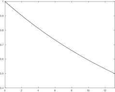
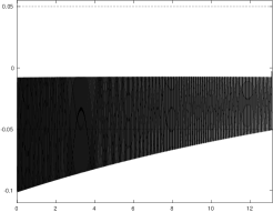
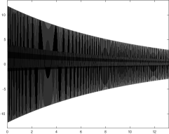
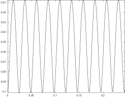
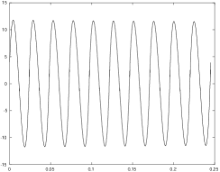
Figure 3.1: $f^{{\cal M}.\alpha}_{\epsilon}(x)$ (left) and its first (center) and second (right) derivatives as a function of $x$ for $\alpha={\scriptstyle\frac{1}{2}}$ and $\epsilon=5.10^{-2}$ (top: $x\in[0,x_{k_{\epsilon,\alpha}}]$; bottom: $x\in[0,x_{10}]$). Horizontal dotted lines indicate values of $-\epsilon$ and $\epsilon$ in the central top graph.

Lemma 3.1

The function $f^{{\cal M}.\alpha}_{\epsilon}$ defined above on the interval $[0,x_{k_{\epsilon,\alpha}}]$ can be extended to a function from IR to IR satifying A.$\alpha$ and whose range is bounded independently of $\alpha$ and $\epsilon$.

• Proof.    We start by showing that, on

  $$[0,x_{k_{\epsilon,\alpha}}]=\bigcup_{k\in{\cal K}}[x_{k},x_{k}+s_{k}],$$

  $f^{{\cal M}.\alpha}_{\epsilon}$ is bounded in absolute value independently of $\epsilon$ and $\alpha$, twice continuously differentiable with Lipschitz continuous gradient and $\alpha$-Hölder continous Hessian. Recall first (3.10) provide that $f^{{\cal M}.\alpha}_{\epsilon}$ is twice continuously differentiable by construction on $[0,x_{k_{\epsilon,\alpha}}]$. It thus remains to investigate the gradient’s Lipschitz continuity and Hessian’s $\alpha-$Hölder continuity, as well as whether $|f^{{\cal M}.\alpha}_{\epsilon}(x)|$ is bounded on this interval.

  Defining now

  $$\pi_{k}\stackrel{{\scriptstyle\rm def}}{{=}}\frac{\theta_{k}}{2}\frac{2f_{k}-1}{f_{k}}\in[0,{\scriptstyle\frac{1}{2}}\theta_{k}]\;\;\mbox{ and }\;\;\phi(\theta)\stackrel{{\scriptstyle\rm def}}{{=}}2-\frac{1}{\theta}\in[2-\frac{\kappa_{\lambda}}{1-\kappa_{rg}},1+\kappa_{rg}]$$ (3.14)

  (where we used (3.4) and (3.6)), we obtain from (3.2), (3.3), (3.6) and (3.13), that, for $k\in{\cal K}$,

  $$\begin{array}[]{llll}|c_{3,k}|s_{k}^{2}&\!=\epsilon f_{k}\left(20-\frac{\displaystyle 10}{\displaystyle\theta_{k}}-2\theta_{k}\right)-\epsilon^{\frac{3+2\alpha}{1+\alpha}}(4+\pi_{k})&\leq\epsilon\left[10|\phi(\theta)|+2\theta+\frac{9}{2}\epsilon^{\frac{2+\alpha}{1+\alpha}}\right]&={\cal O}(\epsilon),\\ |c_{4,k}|s_{k}^{3}&\!=\epsilon f_{k}\left(\frac{\displaystyle 15}{\displaystyle\theta_{k}}-30+\theta_{k}\right)+\epsilon^{\frac{3+2\alpha}{1+\alpha}}(7+2\pi_{k})&\leq\epsilon\left[15|\phi(\theta)|+\theta+8\epsilon^{\frac{2+\alpha}{1+\alpha}}\right]&={\cal O}(\epsilon),\\ |c_{5,k}|s_{k}^{4}&\!=\epsilon f_{k}\left(12-\frac{\displaystyle 6}{\displaystyle\theta_{k}}\right)-\epsilon^{\frac{3+2\alpha}{1+\alpha}}(3+\pi_{k})&\leq\epsilon\left[6|\phi(\theta)|+\frac{7}{2}\epsilon^{\frac{2+\alpha}{1+\alpha}}\right]&={\cal O}(\epsilon),\end{array}$$ (3.15)

  where we also used $\epsilon\leq 1$ and (3.4). To show that the Hessian of $f^{{\cal M}.\alpha}_{\epsilon}$ is globally $\alpha-$Hölder continuous on $[0,x_{k_{\epsilon,\alpha}}]$, we need to verify that (2.8) holds for all $x,y$ in this interval. From (3.10), this is implied by

  $$|p^{{}^{\prime\prime\prime}}(s)|\leq c|s|^{-1+\alpha},\;\;\mbox{for all $s\in[0,s_{k}]$ and $k\in{\cal K}$,}\;\;$$ (3.16)

  for some $c>0$ independent of $\epsilon$, $s$ and $k$. We have from the expression of $p_{k}$ and $s\in[0,s_{k}]$ that

  $$\begin{array}[]{lcl}|p_{k}^{{}^{\prime\prime\prime}}(s)|\cdot|s|^{1-\alpha}&\leq&(6|c_{3,k}|+24|c_{4,k}|s_{k}+60|c_{5,k}|s_{k}^{2})s_{k}^{1-\alpha}\\[4.30554pt] &=&(6|c_{3,k}|s_{k}^{2}+24|c_{4,k}|s_{k}^{3}+60|c_{5,k}|s_{k}^{4})s_{k}^{-(1+\alpha)}.\end{array}$$ (3.17)

  The boundedness of this last right-hand side on $[0,x_{k_{\epsilon,\alpha}}]$ , and thus the $\alpha$-Hölder continuity of the Hessian of $f^{M}$, then follow from (3.15), (3.6) and (3.4).

  Similarly, to show that the gradient of $f^{M}$ is globally Lipschitz continuous in $[0,x_{k_{\epsilon,\alpha}}]$ is equivalent to proving that $p_{k}^{{}^{\prime\prime}}(s)$ is uniformly bounded above on the interval $[0,s_{k}]$ for $k\in{\cal K}$. Since $s_{k}>0$, we have

  $$\begin{array}[]{lcl}|p_{k}^{{}^{\prime\prime}}(s)|&\leq&2|c_{2,k}|+6|c_{3,k}|s_{k}+12|c_{4,k}|s_{k}^{2}+20|c_{5,k}|s_{k}^{3}\\[4.30554pt] &=&2|c_{2,k}|+(6|c_{3,k}|s_{k}^{2}+12|c_{4,k}|s_{k}^{3}+20|c_{5,k}|s_{k}^{4})s_{k}^{-1}.\end{array}$$ (3.18)

  Then the third part of (3.3) and the bounds $\epsilon\leq 1$, (3.15), (3.12), (3.6) and (3.4) again imply the boundedness of the last right-hand side on $[0,x_{k_{\epsilon,\alpha}}]$, as requested. Finally, the fact that $|f^{{\cal M}.\alpha}_{\epsilon}|$ is bounded on $[0,x_{k_{\epsilon,\alpha}}]$ results from the observation that, on the interval $[0,s_{k}]$ with $k\in{\cal K}$,

  $$|p_{k}(s)|\leq f_{k}+|g_{k}||s_{k}|+{\scriptstyle\frac{1}{2}}|H_{k}|\,|s_{k}|^{2}+(|c_{3,k}|s_{k}^{2}+|c_{4,k}|s_{k}^{3}+|c_{5,k}|s_{k}^{4})s_{k}$$

  from which a finite bound $a$ independent from $\alpha$ and $\epsilon$ again follows from $\epsilon\leq 1$, (3.3), (3.10), (3.15), (3.12), (3.6) and (3.4). We have thus proved that $f^{{\cal M}.\alpha}_{\epsilon}$ satisfies the desired properties on $[0,x_{k_{\epsilon,\alpha}}]$.

  We may then smoothly prolongate $f^{{\cal M}.\alpha}_{\epsilon}$ for $x\in\hbox{I\hskip-2.0ptR}$, for instance by defining two additional interpolation intervals $[x_{-1},x_{0}]=[-1,0]$ and $[x_{k_{\epsilon,\alpha}},x_{k_{\epsilon,\alpha}}+1]$ with end conditions

  $$f_{-1}=1,\;\;\;\;f_{k_{\epsilon,\alpha}+1}=f_{k_{\epsilon,\alpha}}\;\;\mbox{and}\;\;g_{-1}=H_{-1}=g_{k_{\epsilon,\alpha}+1}=H_{k_{\epsilon,\alpha}+1}=0,$$

  and setting

  $$f^{{\cal M}.\alpha}_{\epsilon}(x)=\left\{\begin{array}[]{ll}1&\;\;\mbox{for }\;\;x\leq-1,\\ p_{k}(x-x_{k})+f_{k+1}&\;\;\mbox{for }\;\;x\in[x_{k},x_{k+1}]\;\;\mbox{and}\;\;k\in\{-1,\ldots,k_{\epsilon,\alpha}\},\\ f^{{\cal M}.\alpha}_{\epsilon}(x_{k_{\epsilon,\alpha}})&\;\;\mbox{for }\;\;x\geq x_{k_{\epsilon,\alpha}}+1,\\ \end{array}\right.$$

  which subsumes (3.10). Using arguments similar to those used above, it is easy to verify from (3.12), (3.13) and $s_{-1}=s_{k_{\epsilon,\alpha}}=1$ that all desired properties are maintained. $\Box$

We formulate the results of this development in the following theorem.

Theorem 3.2

For every $\epsilon\in(0,1)$, every $\alpha\in[0,1]$ and every method in ${\cal M}.\alpha$, a function $f^{{\cal M}.\alpha}_{\epsilon}$ satisfying A.$\alpha$ with values in a bounded interval independent of $\epsilon$ and $\alpha$ can be constructed, such, when applied to $f^{{\cal M}.\alpha}_{\epsilon}$, the considered method terminates exactly at iteration $$k_{\epsilon,\alpha}=\left\lceil\epsilon^{-\frac{2+\alpha}{1+\alpha}}\right\rceil.$$ with the first iterate $x_{k_{\epsilon,\alpha}}$ such that $\|\nabla_{x}f^{{\cal M}.\alpha}_{\epsilon}(x_{k_{\epsilon,\alpha}})\|\leq\epsilon$.

Note that the prolongation of $f^{{\cal M}.\alpha}_{\epsilon}(x)$ to $x\geq 0$ suggested as an example in the proof of Lemma 3.1 admits an isolated finite global minimizer. Indeed, since the $g_{k_{\epsilon,\alpha}}<0$, there must be a value lower than $f(x_{k_{\epsilon,\alpha}})$ in $(x_{k_{\epsilon,\alpha}},x_{k_{\epsilon,\alpha}}+1)$, and thus the global minimizer must lie in one of the constructed sub-intervals in $(-1,x_{k_{\epsilon,\alpha}+1})$; since $f^{{\cal M}.\alpha}_{\epsilon}(x)$ is quintic (and not constant) in each of these, the global minimizer must therefore be isolated.

3.2 The inexact Newton’s method

It is interesting that the technique developed in the previous subsection can also be used to derive an ${\cal O}\left(\epsilon^{-2}\right)$ lower bound on worst-case evaluation complexity for an inexact Newton’s method applied to a function having Lipschitz continuous Hessians on the path of iterates. This is stronger than using Theorem 3.2 above for $\alpha=1$, as it would result in a weaker ${\cal O}\left(\epsilon^{-3/2}\right)$ lower bound, or for $\alpha=0$ as it would then only guarantee bounded Hessians. In the spirit of [15], this new function is constructed by extending to $\hbox{I\hskip-2.0ptR}^{2}$ the unidimensional $f^{{\cal M}.0}_{\epsilon}(x)$ obtained in the previous section for the specific choice $M_{k}=0$, which then ensures that $\theta_{k}\in[1-\kappa_{rg},1+\kappa_{rg}]$ for all $k$ (see (3.5) and (3.6)). The proposed extension is of the form

$$h^{N}_{\epsilon}(x,y)\stackrel{{\scriptstyle\rm def}}{{=}}f^{{\cal M}.0}_{\epsilon}(x)+u_{\epsilon}(y),$$ (3.19)

where we still have to specify the univariate function $u_{\epsilon}$ such that Newton’s method applied to $u_{\epsilon}$ converges with large steps. In order to define it, we start by redefining

$$k_{\epsilon}=k_{\epsilon,0}=\lceil\epsilon^{-2}\rceil\;\;\mbox{ and }\;\;{\cal K}=\{0,\ldots,k_{\epsilon}\}.$$

Then we set, for $k\in{\cal K}$,

$$u_{k}=1-{\scriptstyle\frac{1}{2}}k\epsilon^{2},\;\;\;\;g_{k}^{u}=-2\epsilon^{2}u_{k},\;\;\;\;H_{k}^{u}=2|g_{k}^{u}|u_{k}>0,$$ (3.20)

and

$$s_{k}^{u}=\frac{\nu_{k}}{2u_{k}}\;\;\mbox{with}\;\;\nu_{k}\in\left[1-\kappa_{rg},1+\kappa_{rg}\right]\;\;\mbox{and}\;\;u_{k}\in[{\scriptstyle\frac{1}{2}},1],$$ (3.21)

this definition allowing for

$$H_{k}^{u}s_{k}^{u}=-g_{k}^{u}+r_{k}^{u}\;\;\mbox{ with }\;\;|r_{k}^{u}|\leq\kappa_{rg}|g^{u}_{k}|.$$

(Remember that $M_{k}=0$ because we are considering Newton’s method.) Note that sufficient decrease is obtained in manner similar to (3.7)-(3.8), because of (3.20), (3.21) and $\lambda_{k}=0$, yielding that $u_{k}-u_{k+1}\geq-(g_{k}^{u}s_{k}^{u}+{\scriptstyle\frac{1}{2}}H_{k}^{u}(s_{k}^{u})^{2})/(1+\kappa_{rg})$. Setting now $y_{0}=0$ and $y_{k+1}=y_{k}+s_{k}^{u}$ for $k\in\{1,\ldots,k_{\epsilon}\}$, we may then, as in Section 3.1, define

$$u_{\epsilon}(y)=p^{u}_{k}(y-y_{k})+u_{k+1}\;\;\mbox{for $y\in[y_{k},y_{k+1}]$ and $k=0,\ldots,k_{\epsilon}-1$,}\;\;$$ (3.22)

where $p^{u}_{k}$ is a fifth degree polynomial interpolating the values and derivatives given by (3.20) on the interval $[0,s_{k}^{u}]$. We then obtain the following result.

Theorem 3.3

For every $\epsilon\in(0,1)$, there exists a function $h^{N}_{\epsilon}$ with Lipschitz continuous gradient and Lipschitz continuous Hessian along the path of iterates $\cup_{k=0}^{k_{\epsilon}-1}[x_{j},x_{j+1}]$, and with values in a bounded interval independent of $\epsilon$, such that, when applied to $h^{N}_{\epsilon}$, Newton’s terminates exactly at iteration $$k_{\epsilon}=\left\lceil\epsilon^{-2}\right\rceil$$ with the first iterate $x_{k_{\epsilon}}$ such that $\|\nabla_{x}f^{{\cal M}.\alpha}_{\epsilon}(x_{k_{\epsilon}})\|\leq\epsilon\sqrt{1+\epsilon^{2}}$.

• Proof.    One easily verifies from (3.20), (3.21) and (3.13) that the interpolation coefficients, now denoted by $|d_{i,k}|$, are bounded for all $k\in\{0,\ldots,k_{\epsilon}-1\}$ and $i\in\{0,\ldots,5\}$. This observation and (3.21) in turn guarantee that $u_{\epsilon}$ and all its derivatives (including the third) remain bounded on each interval $[0,s_{k}^{u}]$ by constants independent of $\epsilon$. As in Lemma 3.1, we next extend $u_{\epsilon}$ to the whole of IR while preserving this property. We then construct $h^{N}$ using (3.19). From the properties of $f^{{\cal M}.0}_{\epsilon}$ and $u_{\epsilon}$, we deduce that $h^{N}_{\epsilon}$ is twice continuously differentiable and has a range bounded independently of $\epsilon$. Moreover, it satisfies A.0. When applied on $h^{N}_{\epsilon}(x,y)$, Newton’s generates the iterates $(x_{k},y_{k})$ and its gradient at the $k_{\epsilon}$-th iterate is $(\epsilon,\epsilon^{2})$ so that $\|\nabla h^{N}(x_{k_{\epsilon}},y_{k_{\epsilon}})\|=\epsilon\sqrt{1+\epsilon^{2}}$, prompting termination. Before that, the algorithm generates the steps $(s_{k},s_{k}^{u})$, where, because both $f_{k}$ and $u_{k}$ belong to $[{\scriptstyle\frac{1}{2}},1]$ and because of (3.6) with $\alpha=0$,

  $$s_{k}\in[\epsilon(1-\kappa_{rg}),2\epsilon(1+\kappa_{rg})]\;\;\mbox{ and }\;\;s_{k}^{u}\in[1-\kappa_{rg},2(1+\kappa_{rg})].$$ (3.23)

  Thus the absolute value of the third derivative of $h^{N}_{\epsilon}(x,y)$ is given, for $(x,y)$ in the $k$-th segment of the path of iterates, by

  $$\begin{array}[]{lcl}\lx@intercol\@ADDCLASS{ltx_eqn_lefteqn}$\displaystyle\frac{1}{\|(s_{k},s_{k}^{u})\|}\Big{|}p_{k}^{{}^{\prime\prime\prime}}(x-x_{k})s_{k}^{3}+(p_{k}^{u})^{{}^{\prime\prime\prime}}(y-y_{k})(s_{k}^{u})^{3}\Big{|}$\mbox{}\hfil\lx@intercol&&\\[5.16663pt] &\;\;\;\;\;\;\;\;\leq&\frac{\displaystyle 1}{\displaystyle 1-\kappa_{rg}}\,\Big{[}|p_{k}^{{}^{\prime\prime\prime}}(x-x_{k})|s_{k}^{3}+|(p_{k}^{u})^{{}^{\prime\prime\prime}}(y-y_{k})|(s_{k}^{u})^{3}\Big{]}\\[5.16663pt] &\;\;\;\;\;\;\;\;=&\frac{\displaystyle 1}{\displaystyle 1-\kappa_{rg}}\,\Big{[}\,\Big{(}6|c_{3,k}|+24|c_{4,k}|s_{k}+60|c_{5,k}|s_{k}^{2}\Big{)}s_{k}^{3}\\[5.16663pt] &&\;\;\;\;\;\;\;\;\;\;\;\;\;\;+\Big{(}6|d_{3,k}|+24|d_{4,k}|s_{k}^{u}+60|d_{5,k}|(s_{k}^{u})^{2}\Big{)}(s_{k}^{u})^{3}\Big{]}\\[5.16663pt] &\;\;\;\;\;\;\;\;=&\frac{\displaystyle 1}{\displaystyle 1-\kappa_{rg}}\,\Big{[}\,\Big{(}6|c_{3,k}|s_{k}^{2}+24|c_{4,k}|s_{k}^{3}+60|c_{5,k}|s_{k}^{4}\Big{)}s_{k}\\[5.16663pt] &&\;\;\;\;\;\;\;\;\;\;\;\;\;\;+6|d_{3,k}|(s_{k}^{u})^{3}+24|d_{4,k}|(s_{k}^{u})^{4}+60|d_{5,k}|(s_{k}^{u})^{5}\Big{]},\end{array}$$ (3.24)

  where we used the fact that $\|(s_{k},s_{k}^{u})\|\geq\|s_{k}^{u}\|.$ and (3.23). But, in view of (3.15), (3.14) with $\theta_{k}\in[1-\kappa_{rg},1+\kappa_{rg}]$, (3.23), $\epsilon\leq 1$ and the boundedness of the $d_{i,k}$, the last right-hand side of (3.24) is bounded by a constant independent of $\epsilon$. Thus the third derivative of $h^{N}_{\epsilon}(x,y)$ is bounded on every segment by the same constant, and, as a consequence, the Hessian of $h^{N}_{\epsilon}(x,y)$ is Lipschitz continuous of each segment, as desired. $\Box$

Note that the same result also holds for any method in ${\cal M}.0$ with $M_{k}$ small enough to guarantee that $s_{k}$ is bounded away from zero for all $k$.

4 Complexity and optimality for methods in ${\cal M}.\alpha$

We now consider the consequences of the examples derived in Section 3 on the evaluation complexity analysis of the various methods identified in Section 2 as belonging to ${\cal M}.\alpha$.

4.1 Newton’s method.

First note that the third part of (3.3) ensures that $H_{k}>0$ so that the Newton iteration is well-defined for the choice (2.23). This choice corresponds to setting $\theta_{k}=1$ for all $k\geq 0$ in the example of Section 3. So we first conclude from Theorem 3.2 that Newton’s method may require $\epsilon^{-(2+\alpha)/(1+\alpha)}$ evaluations when applied on the resulting objective function $f^{{\cal M}.\alpha}_{\epsilon}$ satisfying A.$\alpha$ to generate $|g_{k}|\leq\epsilon$. However, Theorem 3.3 provides the stronger result that it may in fact require $\epsilon^{-2}$ evaluations (as a method in ${\cal M}.0$) for nearly the same task (we traded Lipschitz continuity of the Hessian on the whole space for that along the path of iterates). As a consequence we obtain that Newton’s method is not optimal in ${\cal M}.\alpha$ as far as worst-case evaluation complexity is concerned.

The present results also improves on the similar bound given in [19], in that the objective function on Sections 3.1 and 3.2 ensure the existence of a lower bound $f_{\rm low}$ on $f^{{\cal M}.\alpha}_{\epsilon}(x)$ such that $f^{{\cal M}.\alpha}_{\epsilon}(x_{0})-f_{\rm low}$ is bounded, while the latter difference is unbounded in [19] (for $\alpha\in\{0,1\}$) as the number of iterations approaches $\epsilon^{-2}$. We will return to the significance of this observation when discussing regularization methods.

Since the steepest-descent method is known to have a worst-case evaluation complexity of ${\cal O}\left(\epsilon^{-2}\right)$ when applied on functions having Lipschitz continuous gradients [61, p. 29] , Theorem 3.3 shows that Newton’s method may, in the worst case, converge as slowly as steepest descent in the worst case. Moreover, we show in Appendix A1 that the quoted worst-case evaluation complexity bound for steepest descent is sharp, which means that steepest-descent and Newton’s method are undistinguishable from the point of view of worst-case complexity orders.

Note also that if the Hessian of the objective is unbounded, and hence, we are outside of the class A.$0$, the worst-case evaluation complexity of Newton’s method worsens, and in fact, it may be arbitrarily bad [15].

4.2 Cubic and other regularizations.

Recalling our discussion of the $(2+\alpha)$-regularization method in Section 2.2, we first note, in the example of Section 3.1, that, because of (2.2) and (2.3), $s_{k}$ is a minimizer of the model (2.6) with $\beta_{k}=\lambda_{k}$ at iteration $k$, in that

$$m_{k}(s_{k})=f^{{\cal M}.\alpha}_{\epsilon}(x_{k}+s_{k})=f_{k+1}$$ (4.1)

for $k\in{\cal K}$. Thus every iteration is successful as the objective function decrease exactly matches decrease in the model. Hence the choice $\sigma_{k}=\sigma>0$ for all $k$ is allowed by the method, and thus $\lambda_{k}=\sigma\|s_{k}\|^{2+\alpha}$ satisfies (2.3) and (2.4). Theorem 3.2 then shows that this method may require at least $\epsilon^{-(2+\alpha)/(1+\alpha)}$ iterations to generate an iterate with $|g_{k}|\leq\epsilon$. This is important as the upper bound on this number of iterations was proved in [17] to be

$$O\Big{(}[f(x_{0})-f_{\rm low})]\,\epsilon^{-\frac{2+\alpha}{1+\alpha}}\Big{)}$$ (4.2)

where $f_{\rm low}$ is any lower bound of $f(x)$. Since we have that $f(x_{0})-f_{\rm low}$ is a fixed number independent of $\epsilon$ for the example of Section 3.1, this shows that the ratio

$$\rho_{\rm comp}\stackrel{{\scriptstyle\rm def}}{{=}}\frac{\;\;\mbox{upper bound on the worst-case evaluation complexity}\;\;}{\;\;\mbox{lower bound on the worst-case evaluation complexity}\;\;}$$ (4.3)

for the $(2+\alpha)$-regularization method is bounded independently of $\epsilon$ and $\alpha$. Given that (4.2) involves an unspecified constant, this is the best that can be obtained as far as the order in $\epsilon$ is concerned, and yields the following important result on worst-case evaluation complexity.

Theorem 4.1

When applied to a function satisfying A.$\alpha$, the $(2+\alpha)$-regularization method may require at most (4.2) function and derivatives evaluations. Moreover this bound is sharp (in the sense that $\rho_{\rm comp}$ is bounded independently of $\epsilon$ and $\alpha$) and the $(2+\alpha)$-regularization method is optimal in ${\cal M}.\alpha$.

• Proof.   The optimality of the $(2+\alpha)$-regularization method within ${\cal M}.\alpha$ results from the observation that the example of Section 3 implies that no method in ${\cal M}.\alpha$ can have a worst-case evaluation complexity of a better order. $\Box$

In particular, the cubic regularization method is optimal for smooth optimization problems with Lipschitz continuous second derivatives. As we have seen above, this is in contrast with Newton’s method.

Note that Theorem 4.1 as stated does not result from the statement in [19] that the bound (4.2) is “essentially sharp”. Indeed this latter statement expresses the fact that, for any $\tau>0$, there exists a function independent of $\epsilon$, on which the relevant method may need at least $\epsilon^{-3/2+\tau}$ evaluations to terminate with $|g_{k}|\leq\epsilon$. But, for any fixed $\epsilon$, the value of $f(x_{0})-f_{\rm low}$ tends to infinity when, in the example of that paper, the number of iterations to termination approaches $\epsilon^{-3/2}$ as $\tau$ goes to zero. As a consequence, the numerator of the ratio (4.3), that is (4.2), and $\rho_{\rm comp}$ itself are unbounded for that example. Theorem 4.1 thus brings a formal improvement on the conclusions of [19].

4.3 Goldfeld-Quandt-Trotter

Recalling (2.29), we can set $\omega_{k}=\omega$ in the algorithm as every iteration is successful due to (4.1) which, with (3.3) and $f_{k}\in[{\scriptstyle\frac{1}{2}},1]$ gives that $\lambda_{k}+\lambda_{\min}(H_{k})\leq\omega|g_{k}|^{\frac{\alpha}{1+\alpha}}$, which is in agreement with (2.5) and (2.4). Thus the lower bound of $\epsilon^{-(2+\alpha)/(1+\alpha)}$ iterations for termination also applies to this method.

An upper bound on the worst-case evaluation complexity for the GQT method can be obtained by the following argument. We first note that, similarly to regularization methods, we can bound the total number of unsuccessful iterations as a constant multiple of the successful ones, provided $\omega_{k}$ is chosen such that (2.32) holds. Moreover, since $f$ satisfies A.$\alpha$, its Hessian is bounded above by (2.9). In addition, we have noted in Section 2.2 that $\|g_{k}\|$ is also bounded above. In view of (2.29) and (2.39), this in turn implies that $\|H_{k}+\lambda_{k}I\|$ is also bounded above. Hence we obtain from (2.33) that $\|s_{k}\|\geq\kappa_{GQT}\|g_{k}\|\geq\kappa_{GQT}\,\epsilon$ for some $\kappa_{QGT}>0$, as along as termination has not occurred. This last bound and (2.37) then give that GQT takes at most ${\cal O}\left((f(x_{0})-f_{\rm low})\epsilon^{-\frac{\alpha}{1+\alpha}-2}\right)$ iterations, which is worse than (4.2) for $\alpha>0$. Note that this bound improves if only Newton steps are taken (i.e. $\lambda_{k}=0$ is chosen for all $k\geq 0$), to be of the order of (4.2); however, this cannot be assumed in the worst-case for nonconvex functions. In any case, it implies that the GQT method is not optimal in ${\cal M}.\alpha$.

4.4 Trust-region methods

Recall the choices (2.41) we make in this case. If $\lambda_{k}=0$, the trust-region constraint $\|s\|\leq\Delta_{k}$ is inactive at $s_{k}$, in which case, $s_{k}$ is the Newton step. If we make precisely the choices we made for Newton’s method above, choosing $\Delta_{0}$ such that $\Delta_{0}>|s_{0}|$ implies that the Newton step will be taken in the first and in all subsequent iterations since each iteration is successful and then $\Delta_{k}$ remains unchanged or increases while the choice (3.6) implies that $s_{k}$ decreases. Thus the trust-region approach, through the Newton step, has a worst-case evaluation complexity when applied to $f^{{\cal M}.\alpha}_{\epsilon}$ which is at least that of the Newton’s method, namely $\epsilon^{-2}$.

4.5 Linesearch methods

Because the examples of Sections 3.1 and 3.2 are valid for $r_{k}=0$ which corresponds to $\mu_{k}=1$ for all $k$, and because this stepsize is acceptable since $f(x_{k+1})=m_{k}(s_{k})$, we deduce that at least $\epsilon^{-\frac{2+\alpha}{1+\alpha}}$ iterations and evaluations may be needed for the linesearch variants of any method in ${\cal M}.\alpha$ applied to a function satisfying A.$\alpha$, and that $\epsilon^{-2}$ evaluations may be needed for the linesearch variant of Newton’s method applied on a function satisfying A.$0$. Thus the conclusions drawn regarding their (sub-)optimality in terms of worst-case evaluation complexity are not affected by the use of a linesearch.

5 The Curtis-Robinson-Samadi class

We finally consider a class of methods recently introduced in [36], which we call the CRS class. This class depends on the parameters $0<\underline{\sigma}\leq\bar{\sigma}$, $\eta\in(0,1)$ and two non-negative accuracy thresholds $\kappa_{1}$ and $\kappa_{2}$. It is defined as follows. At the start, adaptive regularization thresholds are set according to

$$\sigma^{L}_{0}=0\;\;\mbox{and}\;\;\sigma^{U}_{0}=\bar{\sigma}.$$ (5.1)

Then for each iteration $k\geq 0$, a step $s_{k}$ from the current iterate $x_{k}$ and a regularization parameter $\lambda_{k}\geq 0$ are chosen to satisfy

$$(H_{k}+\lambda_{k}I)s_{k}=-g_{k}+r_{k},$$ (5.2)

$$\sigma_{k}^{L}\|s_{k}\|\leq\lambda_{k}\leq\sigma_{k}^{U}\|s_{k}\|,$$ (5.3)

$$s_{k}^{T}r_{k}\leq{\scriptstyle\frac{1}{2}}s_{k}^{T}(H_{k}+\lambda_{k}I)s_{k}+{\scriptstyle\frac{1}{2}}\kappa_{1}\|s_{k}\|^{3},$$ (5.4)

and

$$\|r_{k}\|\leq\lambda_{k}\|s_{k}\|+\kappa_{2}\|s_{k}\|^{2}.$$ (5.5)

The step is then accepted, setting $x_{k+1}=x_{k}+s_{k}$, if

$$\rho_{CRS}=\frac{f(x_{k})-f(x_{k}+s_{k})}{\|s_{k}\|^{3}}\geq\eta$$ (5.6)

or rejected otherwise. In the first case, the regularization thresholds are reset according to (5.1). If $s_{k}$ is rejected, $\sigma^{L}_{k}$ and $\sigma^{U}_{k}$ are updated by a simple mechanism (using $\underline{\sigma}$) which is irrelevant for our purpose here. The algorithm is terminated as soon as an iterate is found such that $\|g_{k}\|\leq\epsilon$.

Observe that (5.2) corresponds to inexactly minimizing the regularized model (2.6) and that (5.5) is very similar to the subproblem termination rule of [10].

An upper bound of ${\cal O}\left(\epsilon^{-3/2}\right)$ is proved in [36, Theorem 17] for the worst-case evaluation complexity of the methods belonging to the CRS class. It is stated in [36] that both ARC [54, 72, 63, 16, 17] and TRACE [37] belong to the class, although the details are not given.

Clearly, the CRS class is close to ${\cal M}.1$, but yet differs from it. In particular, no requirement is made that $H_{k}+\lambda_{k}I$ be positive semi-definite but (5.4) is required instead, there is no formal need for the step to be bounded and (5.5) combined with (5.3) is slightly more permissive than the second part of (2.2). We now define CRS_a, a sub-class of the CRS class of methods, as the set of CRS methods for which (5.5) is strengthened to become

$$\|r_{k}\|\leq\min\Big{[}\kappa_{rg}\|g_{k}\|,\lambda_{k}\|s_{k}\|+\kappa_{2}\|s_{k}\|^{2}\Big{]}\;\;\mbox{ with }\;\;\kappa_{rg}<1.$$ (5.7)

(in a manner reminiscent of the second part of (2.2)) and such that

$$2\eta(1+\kappa_{rg})^{3}\leq 1$$ (5.8)

(a mild technical condition whose need will become apparent below). We claim that, for any choice of method in the CRS_a class and termination threshold $\epsilon$, we can construct a function satisfying A.1 such that the considered CRS_a method terminates in exactly $\left\lceil\epsilon^{-3/2}\right\rceil$ iterations and evaluations. This achieved simply by showing that the generated sequences of iterates, function, gradient and Hessian values belong to those detailed in the example of Section 3.1.

We now apply a method of the CRS_a class for a given $\epsilon>0$, and first consider an iterate $x_{k}$ with associated values $f_{k}$, $g_{k}$ and $H_{k}$ given by (3.3) for $\alpha=1$, that is

$$f_{0}=1,\;\;\;\;f_{k}=f_{0}-{\scriptstyle\frac{1}{2}}k\epsilon^{3/2},\;\;\;\;g_{k}=-2\epsilon f_{k}\;\;\mbox{and}\;\;H_{k}=4\epsilon^{1/2}f_{k}^{2};$$ (5.9)

Suppose that

$$\sigma_{k}^{L}=0\;\;\mbox{ and }\;\;\sigma_{k}^{U}=\bar{\sigma}$$ (5.10)

(as is the case by definition for $k=0$), and let

$$s_{k}=\theta_{k}\frac{\epsilon^{1/2}}{2f_{k}}\;\;\;\;(\theta_{k}>0)$$ (5.11)

be an acceptable step for an arbitrary method in the CRS_a class. Now, because of (5.10), (5.3) reduces to

$$\lambda_{k}\in[0,\bar{\sigma}|s_{k}|]=\left[0,\bar{\sigma}\theta_{k}\frac{\epsilon^{1/2}}{2f_{k}}\right]$$ (5.12)

and, given that $H_{k}>0$ because of (5.9), this in turn implies that $H_{k}+\lambda_{k}>0$. Condition (5.7) requires that

$$|g_{k}+(H_{k}+\lambda_{k})s_{k}|=|r_{k}|\leq\kappa_{rg}|g_{k}|=2\kappa_{rg}\epsilon f_{k}<2\epsilon,$$ (5.13)

where we used the fact that $f_{k}\leq 1$ because of (5.9) and $\kappa_{rg}<1$ because of (5.7). Moreover, (5.13) and (5.12) imply that

$$\frac{2(1-\kappa_{rg})\epsilon f_{k}}{4\epsilon^{1/2}f_{k}^{2}+\bar{\sigma}s_{k}}\leq\frac{|g_{k}|(1-\kappa_{rg})}{H_{k}+\lambda_{k}}\leq s_{k}\leq\frac{|g_{k}|(1+\kappa_{rg})}{H_{k}+\lambda_{k}}\leq\frac{(1+\kappa_{rg})\epsilon^{1/2}}{2f_{k}}.$$ (5.14)

Thus, using (5.11) and the right-most part of these inequalities, we obtain that $\theta_{k}\leq 1+\kappa_{rg}$, which in turn ensures that $s_{k}\leq(1+\kappa_{rg})\epsilon^{1/2}/(2f_{k})$. Substituting this latter bound in the denominator of the left-most part of (5.14) and using (5.11) again with the fact that $f_{k}\geq{\scriptstyle\frac{1}{2}}$ before termination, we obtain that

$$\theta_{k}\in\left[\frac{1-\kappa_{rg}}{1+\bar{\sigma}(1+\kappa_{rg})},1+\kappa_{rg}\right]$$ (5.15)

(note that this is (3.6) with $\kappa_{\lambda}=1+\bar{\sigma}(1+\kappa_{rg})$). We immediately note that $\pi_{k}$ and $\phi(\theta_{k})$ are then both guaranteed to be bounded above and below as in (3.14). (Since this is enough for our purpose, we ignore the additional restriction on $\theta_{k}$ which might result from (5.4).) Using the definitions (5.9) for $k+1$, we may then construct the objective function $f_{\epsilon}^{CRS}$ on the interval $[x_{k},x_{k}+s_{k}]$ by Hermite interpolation, as in Section 3.1. Moreover, using (5.6), (5.9), (5.11), (5.15), $f_{k}\in[{\scriptstyle\frac{1}{2}},1]$ and the condition (5.8), we obtain that

$$\rho_{k}=\frac{\epsilon^{3/2}}{2}\left(\frac{2f_{k}}{\theta_{k}\epsilon^{1/2}}\right)^{3}=\frac{4f_{k}^{3}}{\theta_{k}^{3}}\geq\frac{1}{2(1+\kappa_{rg})^{3}}\geq\eta.$$

Thus iteration $k$ is successful, $x_{k+1}=x_{k}+s_{k}$, $\sigma^{L}_{k+1}=\sigma^{L}_{k}=0$, $\sigma^{U}_{k+1}=\sigma^{U}_{k}=\bar{\sigma}$, and all subsequent iterations of the CRS_a method up to termination follow the same pattern in accordance with (5.9). As in Section 3.1, we may construct $f_{\epsilon}^{CRS}$ on the whole of IR which satisfies A.1 and such that, the considered CRS_a method applied to $f_{\epsilon}^{CRS}$ will terminate in exactly $\lceil\epsilon^{-3/2}\rceil$ iterations and evaluations. This and the ${\cal O}\left(\epsilon^{-3/2}\right)$ upper bound on the worst-case evaluation complexity of CRS methods allow stating the following theorem.

Theorem 5.1

For every $\epsilon\in(0,1)$ and every method in the CRS_a class, a function $f^{CRS}_{\epsilon}$ satisfying A.$1$ with values in a bounded interval independent of $\epsilon$ can be constructed, such that the considered method terminates exactly at iteration $$k_{\epsilon}=\left\lceil\epsilon^{-3/2}\right\rceil$$ with the first iterate $x_{k_{\epsilon}}$ such that $\|\nabla_{x}f^{CRS}_{\epsilon}(x_{k_{\epsilon}})\|\leq\epsilon$. As a consequence, methods in CRS_a are optimal within the CRS class and their worst-case evaluation complexity is, in order, also optimal with respect to that of methods in ${\cal M}.1$.

CRS_a then constitutes a kernel of optimal methods (from the worst-case evaluation complexity point of view) within CRS and ${\cal M}.1$. Methods in CRS but not in CRS_a correspond to very inaccurate minimization of the regularized model, which makes it unlikely that their worst-case evaluation complexity surpasses that of methods in CRS_a. Finally note that, since we did not use (5.4) to construct our example, it effectively applies to a class larger than CRS_a where this condition is not imposed.

6 The algorithm of Royer and Wright

We finally consider the linesearch algorithm proposed in [65, Algorithm 1], which is reminiscent of the double linesearch algorithm of [47] and [34, Section 10.3.1]. From a given iterate $x_{k}$, this algorithm computes a search direction $d_{k}$ whose nature depends on the curvature of the (unregularized) quadratic model along the negative gradient, and possibly computes the left-most eigenpair of the Hessian if this curvature is negative or if the gradient’s norm is small enough to declare first-order stationarity. A linesearch along $d_{k}$ is then performed by reducing the steplength $\alpha_{k}$ from $\alpha_{k}=1$ until

$$f(x_{k}+\alpha_{k}d_{k})\leq f(x_{k})-\frac{\eta}{6}\alpha_{k}^{3}\|d_{k}\|^{3}$$ (6.1)

for some $\eta>0$. The algorithm uses $\epsilon_{g}$ and $\epsilon_{H}$, two different accuracy thresholds for first- and second-order approximate criticality, respectively.

Our objective is now to show that, when applied to the function $f^{{\cal M}.1}_{\epsilon_{g}}$ of Section 3.1 with $\epsilon=\epsilon_{g}$, this algorithm, which we call the RW algorithm, takes exactly $k_{\epsilon_{g},1}=\lceil\epsilon_{g}^{-3/2}\rceil$ iterations and evaluations to terminate with $\|g_{k}\|\leq\epsilon_{g}$.

We first note that (3.3) guarantees that $H_{k}$ is positive definite and, using (3.4), that

$$\frac{g_{k}^{T}H_{k}g_{k}}{\|g_{k}\|^{2}}=4\epsilon_{g}^{1/2}f_{k}^{2}>\epsilon_{g}$$

for $k\in\{0,\ldots,k_{\epsilon_{g},1}\}$. Then, provided

$$\epsilon_{H}\leq\sqrt{\epsilon_{g}},$$ (6.2)

and because $\lambda_{\min}(H_{k})=4\epsilon_{g}^{1/2}f_{k}^{2}>\epsilon_{H}$ (using (3.4) again), the RW algorithm defines the search direction from Newton’s equation $H_{k}d_{k}=-g_{k}$ (which corresponds, as we have already seen, to taking $M_{k}=0=r_{k}$ and thus $\theta_{k}=1$ in the example of Section 3.1). The RW algorithm is therefore, on that example, identical to a linesearch variant of Newton’s method with the specific linesearch condition (6.1). Moreover, using (3.4) once more,

$$f(x_{k})-f(x_{k}+d_{k})=\frac{1}{2}\epsilon_{g}^{3/2}\geq\frac{\eta}{6}\left(\frac{\epsilon_{g}^{1/2}}{2f_{k}}\right)^{3}\geq\frac{\eta}{6}\epsilon_{g}^{3/2}$$

whenever $\eta\leq 3$, an extremely weak condition. Thus (6.1) holds with $\alpha_{k}=1$. We have thus proved that the RW algorithm generates the same sequence of iterates as Newton’s method when applied to $f^{{\cal M}.1}_{\epsilon_{g}}$. The fact that an upper bound of ${\cal O}\left(\epsilon_{g}^{-3/2}\right)$ iterations and evaluations was proved to hold in [65, Theorem 5] then leads us to stating the following result.

Theorem 6.1

Assume that $\eta\in(0,3]$. Then, for every $\epsilon_{g}\in(0,1)$ and $\epsilon_{H}$ satisfying (6.2), a function $f^{{\cal M}.1}_{\epsilon_{g}}$ satisfying A.$1$ with values in a bounded interval (independent of $\epsilon_{g}$ and $\epsilon_{H}$) can be constructed, such that the Royer-Wright algorithm terminates exactly at iteration $$k_{\epsilon_{g}}=\left\lceil\epsilon_{g}^{-3/2}\right\rceil$$ with the first iterate $x_{k_{\epsilon_{g}}}$ such that $\|\nabla_{x}f^{{\cal M}.1}_{\epsilon_{g}}(x_{k_{\epsilon_{g}}})\|\leq\epsilon_{g}$. As a consequence and under assumption (6.2), the first-order worst-case evaluation complexity order of ${\cal O}\left(\epsilon_{g}^{-3/2}\right)$ for this algorithm is sharp and it is (in order of $\epsilon_{g}$), also optimal with respect to that of algorithms in the ${\cal M}.1$ and CRS classes.

7 Conclusions

We have provided lower bounds on the worst-case evaluation complexity of a wide class of second-order methods for reaching approximate first-order critical points of nonconvex, adequately smooth unconstrained optimization problems. This has been achieved by providing improved examples of slow convergence on functions with bounded range independent of $\epsilon$. We have found that regularization algorithms, methods belonging to a subclass of that proposed in [36] and the linesearch algorithm of [65] are optimal from a worst-case complexity point of view within a very wide class of second-order methods, in that their upper complexity bounds match in order the lower bound we have shown for relevant, sufficiently smooth objectives satisfying A.$\alpha$. At this point, the question of whether all known optimal second-order methods share enough design concepts to be made members of a single class remains open.

Note that every iteration complexity bound discussed above is of the order $\epsilon^{-p}$ (for various values of $p>0$) for driving the objective’s gradient below $\epsilon$; thus the methods we have addressed may require an exponential number of iterations $10^{p\cdot k}$ to generate $k$ correct digits in the solution. Also, as our examples are one-dimensional, they fail to capture the problem-dimension dependence of the upper complexity bounds. Indeed, besides the accuracy tolerance $\epsilon$, existing upper bounds depend on the distance to the solution set, that is $f(x_{0})-f_{\rm low}$, and the gradient’s and Hessian’s Lipschitz or Hölder constants, all of which may dependent on the problem dimension. Some recent developments in this respect can be found in [56, 1, 57, 65].

Here we have solely addressed the evaluation complexity of generating first-order critical points, but it is common to require second-order methods for nonconvex problems to achieve second-order criticality. Indeed, upper worst-case complexity bounds are known in this case for cubic regularization and trust-region methods [63, 17, 21], which are essentially sharp in some cases [21]. A lower bound on the whole class of second order methods for achieving second-order optimality remains to be established, especially when different accuracy is requested in the first- and second-order criticality conditions.

Regarding the worst-case evaluation complexity of constrained optimization problems, we have shown [20, 18, 23] that the presence of constraints does not change the order of the bound, so that the unconstrained upper bound for some first- or second-order methods carries over to the constrained case; note that this does not include the cost of solving the constrained subproblems as the latter does not require additional problem evaluations. Since constrained problems are at least as difficult as unconstrained ones, these bounds are also sharp. It remains an open question whether a unified treatment such as the one given here can be provided for the worst-case evaluation complexity of methods for constrained problems.

A1. An example of slow convergence of the steepest-descent method

We show in this paragraph that the steepest-descent method may need at least $\epsilon^{-2}$ iteration to terminate on a function whose range is fixed and independent of $\epsilon$.

We once again follow the methodology used in Section 3.1 and build a unidimensional function $f^{SD}_{\epsilon}$ by Hermite interpolation, such that the steepest-descent method applied to this function takes exactly $k_{\epsilon}=\lceil\epsilon^{-2}\rceil$ iterations and function evaluations to terminate with an iterate $x_{k}$ such that $|g(x_{k})|\leq\epsilon$. Note that, for the sequence of function values to be interpretable as the result of applying the steepest-descent method (using a Goldstein linesearch), we require that, for all $k$,

$$f(x_{k})+\mu_{1}g_{k}^{T}s_{k}\leq f(x_{k}-\mu_{k}g_{k})\leq f(x_{k})+\mu_{2}g_{k}^{T}s_{k}\;\;\mbox{ for constants }\;\;0<\mu_{2}<\mu_{1}<1$$ (A.1)

where, as above, $s_{k}=x_{k+1}-x_{k}$. Keeping this in mind, we define the sequences ${f_{k}}$, ${g_{k}}$, ${H_{k}}$ and ${s_{k}}$ for $k\in\{0,\ldots,k_{\epsilon}-1\}$ by

$$f_{k}=1-{\scriptstyle\frac{1}{2}}k\epsilon^{2}\;\;\;\;g_{k}=-2\epsilon f_{k},\;\;\;\;H_{k}=0,\;\;\;\;r_{k}=0\;\;\mbox{and}\;\;\mu_{k}=\frac{1}{4f_{k}^{2}}\in[{\scriptstyle\frac{1}{4}},1].$$

Note that this last definition ensures that (A.1) holds provided $0<\mu_{2}<{\scriptstyle\frac{1}{2}}<\mu_{1}<1$. It also gives that $s_{k}=\epsilon/(2f_{k})\leq\epsilon<1$. Using these values, it can also be verified that termination occurs for $k=k_{\epsilon}$, that $f^{SD}_{\epsilon}$ defined by (3.10) and Hermite interpolation is twice continuously differentiable on $[0,x_{k_{\epsilon}}]$ and that (3.12) again holds. Since $|g_{k}|\leq\epsilon$, we also obtain that, for $k\in\{0,\ldots,k_{\epsilon}-1\}$,

$$\left|\frac{\Delta f_{k}}{s_{k}^{2}}\right|=2f_{k}^{2}\leq 1,\;\;\;\;\left|\frac{\Delta g_{k}}{s_{k}}\right|=2\epsilon^{2}f_{k}\leq 2\;\;\mbox{and}\;\;\left|\frac{g_{k}}{s_{k}}\right|=4f_{k}^{2}\leq 4.$$

These bounds, $H_{k}=\Delta H_{k}=0$, the first equality of (3.18) and (3.13) then imply that the Hessian of $f^{SD}_{\epsilon}$ is bounded above by a constant independent of $\epsilon$. $f^{SD}_{\epsilon}$ thus satisfies A.$0$ and therefore has Lipchitz continuous gradient. Moreover, since $s_{k}\leq 1$, we also obtain, as in Section 3.1 and 3.2, that $|f^{SD}_{\epsilon}|$ is bounded by a constant independent of $\epsilon$ on $[0,x_{k_{\epsilon}}]$. As above we then extend $f^{SD}_{\epsilon}$ to the whole of IR while preserving A.$0$.

Theorem A.1

For every $\epsilon\in(0,1)$, a function $f^{SD}_{\epsilon}$ satisfying A.$0$ (and thus having Lipschitz continuous gradient) with values in a bounded interval independent of $\epsilon$ can be constructed, such that the steepest-descent method terminates exactly at iteration $$k_{\epsilon}=\left\lceil\epsilon^{-2}\right\rceil$$ with the first iterate $x_{k_{\epsilon}}$ such that $\|\nabla_{x}f^{SD}_{\epsilon}(x_{k_{\epsilon}})|\leq\epsilon$.

As a consequence, the ${\cal O}\left(\epsilon^{-2}\right)$ order of worst-case evaluation complexity is sharp for the steepest-descent method in the sense that the complexity ratio $\rho_{\rm comp}$ is bounded above independently of of $\epsilon$, which improves on the conclusion proposed in [15] for the steepest-descent method.

The top three graphs of Figure A.2 illustrate the global behaviour of the resulting function $f^{N}_{\epsilon}(x)$ and of its first and second derivatives for $x\in[0,x_{k_{\epsilon}}]$, while the bottom ones show more detail of the first 10 iterations. The figure is once more constructed using $\epsilon=5.10^{-2}$ ($k_{\epsilon}=400$).

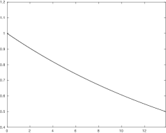
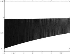
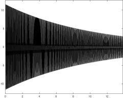
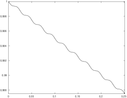
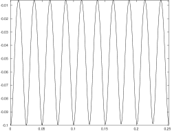
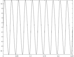
Figure A.2: $f^{SD}_{\epsilon}(x)$ (left) and its first (center) and second (right) derivatives as a function of $x$ for $\epsilon=5.10^{-2}$ (top: $x\in[0,x_{k_{\epsilon,\alpha}}]$; bottom: $x\in[0,x_{10}]$). Horizontal dotted lines indicate values of $-\epsilon$ and $\epsilon$ in the central top graph.

A2. Upper complexity bound for the $(2+\alpha)$-regularization method

The purpose of this paragraph is to to provide some of the missing details in the proof of Lemma 2.5, as well as making explicit the statement made at the end of Section 5.1 in [17] that the $(2+\alpha)$-regularization method needs at most (4.2) iterations (and function/derivatives evaluations) to obtain and iterate $x_{k}$ such that $|g_{k}|\leq\epsilon$.

We start by proving (2.27) following the reasoning of [16, Lem.2.2]. Consider

$$\begin{array}[]{lcl}m_{k}(s)-f(x_{k})&=&g_{k}^{T}s+{\scriptstyle\frac{1}{2}}s^{T}H_{k}s+\frac{1}{2+\alpha}\sigma_{k}\|s\|^{2+\alpha}\\[4.30554pt] &\geq&-\|g_{k}\|\,\|s\|-{\scriptstyle\frac{1}{2}}\|s\|^{2}\,\|H_{k}\|+\frac{1}{2+\alpha}\sigma_{k}\|s\|^{2+\alpha}\\[4.30554pt] &\geq&\left(\frac{1}{3(2+\alpha)}\sigma_{k}\|s\|^{2+\alpha}-\|g_{k}\|\,\|s\|\right)+\left(\frac{2}{3(2+\alpha)}\sigma_{k}\|s\|^{2+\alpha}-{\scriptstyle\frac{1}{2}}\|s\|^{2}\|H_{k}\|\right)\end{array}$$

But then $\frac{2}{3(2+\alpha)}\sigma_{k}\|s\|^{2+\alpha}-\|H_{k}\|\,\|s\|^{2}>0$ if $\|s_{k}\|<(3(2+\alpha)\|H_{k}\|/(4\sigma_{k}))^{\frac{1}{\alpha}}$ while $\frac{1}{3(2+\alpha)}\sigma_{k}\|s\|^{2+\alpha}-\|g_{k}\|\,\|s\|>0$ if $\|s_{k}\|<(3(2+\alpha)\|g_{k}\|/\sigma_{k})^{\frac{1}{1+\alpha}}$. Hence, since $m_{k}(s_{k})<f(x_{k})$, we have that

$$\|s_{k}\|\leq\max\left[\left(\frac{3(2+\alpha)\|H_{k}\|}{4\sigma_{k}}\right)^{\frac{1}{\alpha}},\left(\frac{3(2+\alpha)\|g_{k}\|}{\sigma_{k}}\right)^{\frac{1}{1+\alpha}}\right]$$

which yields (2.27) because $\|H_{k}\|\leq L_{g}$.

We next explicit the worst-case evaluation complexity bounf of Section 5.1 in [17]. Following [16, Lemma 5.2], we start by proving that

$$\sigma_{\max}\stackrel{{\scriptstyle\rm def}}{{=}}c_{\sigma}\max(\sigma_{0},L_{H,\alpha})$$ (A.1)

for some constant $c_{\sigma}$ only dependent on $\alpha$ and algorithm’s parameters. To show this inequality, we deduce from Taylor’s theorem that, for each $k\geq 0$ and some $\xi_{k}$ belonging the the segment $[x_{k},x_{k}+s_{k}]$,

$$f(x_{k}+s_{k})-m_{k}(s_{k})\leq\frac{1}{2}\|H(\xi_{k})-H(x_{k})\|\cdot\|s_{k}\|^{2}-\frac{\sigma_{k}}{2+\alpha}\|s_{k}\|^{2+\alpha}\leq\left(\frac{L_{H,\alpha}}{2}-\frac{\sigma_{k}}{2+\alpha}\right)\|s_{k}\|^{2+\alpha},$$

where, to obtain the second inequality, we employed (2.8) in A.$\alpha$ and $\|\xi_{k}-x_{k}\|\leq\|s_{k}\|$. Thus $f(x_{k}+s_{k})<m_{k}(s_{k})$ whenever $\sigma_{k}>{\scriptstyle\frac{1}{2}}(2+\alpha)L_{H,\alpha}$, providing sufficient descent and ensuring that $\sigma_{k+1}\leq\sigma_{k}$. Taking into account the (possibly large) choice of the regularization parameter at startup then yields (A.1).

We next note that, because of (2.25) and (A.1), (2.11) holds. Moreover, $\kappa(M_{k})=\kappa\left(\sigma_{k}\|s_{k}\|^{\alpha}I\right)=1$. Lemma 2.3 then ensures that (2.16) also holds.

We finally follow [16, Corollary 5.3] to prove the final upper bound on the number of successful iterations (and hence on the number of function and derivatives evaluations). Let ${\cal S}^{\epsilon}_{k}$ index the subset of the first $k$ iterations that are successful and such that $\min[\|g_{k}\|,\|g_{k+1}\|]>\epsilon$, and let $|{\cal S}^{\epsilon}_{k}|$ denote its cardinality. It follows from this definition, (2.11), (2.26) and the fact that sufficient decrease is obtained at successful iterations that, for all $k$ before termination,

$$f(x_{j})-m_{k}(s_{j})\geq\alpha_{\rm S}\epsilon^{\frac{2+\alpha}{1+\alpha}},\;\;\mbox{for all $j\in{\cal S}^{\epsilon}_{k}$,}\;\;$$ (A.2)

for some positive constant $\alpha_{\rm S}$ independent of $\epsilon$. Now, if $f_{\rm low}>-\infty$ is a lower bound on $f(x)$, we have, using the monotonically decreasing nature of $\{f(x_{k})\}$, that

$$\begin{array}[]{lcccl}f(x_{0})-f_{\rm low}&\geq&f(x_{0})-f(x_{k+1})&=&\displaystyle\sum_{j\in{\cal S}^{\epsilon}_{k}}\left[f(x_{j})-f(x_{j+1})\right]\\[4.30554pt] &\geq&\eta_{1}\displaystyle\sum_{j\in{\cal S}^{\epsilon}_{k}}\left[f(x_{j})-m_{k}(s_{j})\right]&\geq&|{\cal S}^{\epsilon}_{k}|\,\eta_{1}\alpha_{\rm S}\,\epsilon^{\frac{2+\alpha}{1+\alpha}},\end{array}$$

where the constant $\eta_{1}\in(0,1)$ defines sufficient decrease. Hence, for all $k\geq 0$,

$$|{\cal S}^{\epsilon}_{k}|\leq\frac{f(x_{0})-f_{\rm low}}{\eta_{1}\alpha_{\rm S}}\,\,\epsilon^{-\frac{2+\alpha}{1+\alpha}}.$$

As a consequence, the $(2+\alpha)$-regularization method needs at most (4.2) successful iterations to terminate. Since it known that, for regularization methods, $k\leq\kappa_{\cal S}|{\cal S}^{\epsilon}_{k}|$ for some constant $\kappa_{\cal S}$ [17, Theorem 2.1] and because every iteration involves a single evaluation, we conclude that the $(2+\alpha)$-regularization method needs at most (4.2) function and derivatives evaluations to produce an iterate $x_{k}$ such that $\|g_{k}\|\leq\epsilon$ when applied to an objective function satisfying A.$\alpha$.

We finally oserve that the statement (made in the proof of Lemma 2.5) that $\|g_{k}\|$ is bounded above immediately follows from this worst-case evaluation complexity bound.

References

• [1] Z. Agarwal, B. Allen-Zhu, B. Bullins, E. Hazan, and T. Ma. Finding approximate local minima for nonconvex optimization in linear time. arXiv:1611.01146, 2016.
• [2] A. Anandkumar and R. Ge. Efficient approaches for escaping high-order saddle points in nonconvex optimization. arXiv.1602.05908, 2016.
• [3] E. Bergou, Y. Diouane, and S. Gratton. On the use of the energy norm in trust-region and adaptive cubic regularization subproblems, April 2017.
• [4] W. Bian and X. Chen. Worst-case complexity of smoothing quadratic regularization methods for non-Lipschitzian optimization. SIAM Journal on Optimization, 23(3):1718–1741, 2013.
• [5] W. Bian and X. Chen. Linearly constrained non-Lipschitzian optimization for image restoration. SIAM Journal on Imaging Sciences, 8:2294–2322, 2015.
• [6] W. Bian, X. Chen, and Y. Ye. Complexity analysis of interior point algorithms for non-Lipschitz and nonconvex minimization. Mathematical Programming, Series A, 149:301–327, 2015.
• [7] T. Bianconcini, G. Liuzzi, B. Morini, and M. Sciandrone. On the use of iterative methods in cubic regularization for unconstrained optimization. Computational Optimization and Applications, 60(1):35–57, 2015.
• [8] T. Bianconcini and M. Sciandrone. A cubic regularization algorithm for unconstrained optimization using line search and nonmonotone techniques. Optimization Methods and Software, 31(5):1008–1035, 2016.
• [9] E. G. Birgin, J. L. Gardenghi, J. M. Martínez, S. A. Santos, and Ph. L. Toint. Evaluation complexity for nonlinear constrained optimization using unscaled KKT conditions and high-order models. SIAM Journal on Optimization, 26(2):951–967, 2016.
• [10] E. G. Birgin, J. L. Gardenghi, J. M. Martínez, S. A. Santos, and Ph. L. Toint. Worst-case evaluation complexity for unconstrained nonlinear optimization using high-order regularized models. Mathematical Programming, Series A, 163(1):359–368, 2017.
• [11] E. G. Birgin and J. M. Martínez. On regularization and active-set methods with complexity for constrained optimization. www.ime.usp.br/ egbirgin/publications/bmnuevogencan_siamformat.pdf, April 2017.
• [12] N. Boumal, P.-A. Absil, and C. Cartis. Global rates of convergence for nonconvex optimization on manifolds. arXiv:1605.08101, 2016.
• [13] Y. Carmon and J. C. Duchi. Gradient descent efficiently finds the cubic-regularized non-convex Newton step. arXiv:1612.00547v2, 2016.
• [14] Y. Carmon, J. C. Duchi, O. Hinder, and A. Sidford. ”Convex until proven guilty”: Dimension-free acceleration of gradient descent on non-convex functions. arXiv:1705.02766v1, 2017.
• [15] C. Cartis, N. I. M. Gould, and Ph. L. Toint. On the complexity of steepest descent, Newton’s and regularized Newton’s methods for nonconvex unconstrained optimization. SIAM Journal on Optimization, 20(6):2833–2852, 2010.
• [16] C. Cartis, N. I. M. Gould, and Ph. L. Toint. Adaptive cubic overestimation methods for unconstrained optimization. Part I: motivation, convergence and numerical results. Mathematical Programming, Series A, 127(2):245–295, 2011.
• [17] C. Cartis, N. I. M. Gould, and Ph. L. Toint. Adaptive cubic overestimation methods for unconstrained optimization. Part II: worst-case function-evaluation complexity. Mathematical Programming, Series A, 130(2):295–319, 2011.
• [18] C. Cartis, N. I. M. Gould, and Ph. L. Toint. On the evaluation complexity of composite function minimization with applications to nonconvex nonlinear programming. SIAM Journal on Optimization, 21(4):1721–1739, 2011.
• [19] C. Cartis, N. I. M. Gould, and Ph. L. Toint. Optimal Newton-type methods for nonconvex optimization. Technical Report naXys-17-2011, Namur Center for Complex Systems (naXys), University of Namur, Namur, Belgium, 2011.
• [20] C. Cartis, N. I. M. Gould, and Ph. L. Toint. An adaptive cubic regularization algorithm for nonconvex optimization with convex constraints and its function-evaluation complexity. IMA Journal of Numerical Analysis, 32(4):1662–1695, 2012.
• [21] C. Cartis, N. I. M. Gould, and Ph. L. Toint. Complexity bounds for second-order optimality in unconstrained optimization. Journal of Complexity, 28:93–108, 2012.
• [22] C. Cartis, N. I. M. Gould, and Ph. L. Toint. On the complexity of the steepest-descent with exact linesearches. Technical Report naXys-16-2012, Namur Center for Complex Systems (naXys), University of Namur, Namur, Belgium, 2012.
• [23] C. Cartis, N. I. M. Gould, and Ph. L. Toint. On the complexity of finding first-order critical points in constrained nonlinear optimization. Mathematical Programming, Series A, 144(1):93–106, 2013.
• [24] C. Cartis, N. I. M. Gould, and Ph. L. Toint. On the evaluation complexity of cubic regularization methods for potentially rank-deficient nonlinear least-squares problems and its relevance to constrained nonlinear optimization. SIAM Journal on Optimization, 23(3):1553–1574, 2013.
• [25] C. Cartis, N. I. M. Gould, and Ph. L. Toint. Improved worst-case evaluation complexity for potentially rank-deficient nonlinear least-Euclidean-norm problems using higher-order regularized models. Technical Report naXys-12-2015, Namur Center for Complex Systems (naXys), University of Namur, Namur, Belgium, 2015.
• [26] C. Cartis, N. I. M. Gould, and Ph. L. Toint. On the evaluation complexity of constrained nonlinear least-squares and general constrained nonlinear optimization using second-order methods. SIAM Journal on Numerical Analysis, 53(2):836–851, 2015.
• [27] C. Cartis, N. I. M. Gould, and Ph. L. Toint. Improved second-order evaluation complexity for unconstrained nonlinear optimization using high-order regularized models. arXiv:1708.04044, 2017.
• [28] C. Cartis, N. I. M. Gould, and Ph. L. Toint. Optimality of orders one to three and beyond: characterization and evaluation complexity in constrained nonconvex optimization. Foundations of Computational Mathematics, (to appear), 2017. DOI:10.1007/s10208-017-9363-y.
• [29] C. Cartis, N. I. M. Gould, and Ph. L. Toint. Second-order optimality and beyond: characterization and evaluation complexity in convexly-constrained nonlinear optimization. Foundations of Computational Mathematics, (to appear), 2017.
• [30] C. Cartis, N. I. M. Gould, and Ph. L. Toint. Universal regularization methods – varying the power, the smoothness and the accuracy. Optimization Methods and Software, (to appear), 2017.
• [31] C. Cartis, Ph. R. Sampaio, and Ph. L. Toint. Worst-case complexity of first-order non-monotone gradient-related algorithms for unconstrained optimization. Optimization, 64(5):1349–1361, 2015.
• [32] C. Cartis and K. Scheinberg. Global convergence rate analysis of unconstrained optimization methods based on probabilistic models. Mathematical Programming, Series A, (to appear), 2017. DOI 10.1007/s10107-017-1137-4.
• [33] X. Chen, Ph. L. Toint, and H. Wang. Partially separable convexly-constrained optimization with non-Lipschitzian singularities and its complexity. arXiv:1704.06919, 2017.
• [34] A. R. Conn, N. I. M. Gould, and Ph. L. Toint. Trust-Region Methods. MPS-SIAM Series on Optimization. SIAM, Philadelphia, USA, 2000.
• [35] F. E. Curtis, D. P. Robinson, and M. Samadi. Complexity analysis of a trust funnel algorithm for equality constrained optimization. Technical Report 16T-03, ISE/COR@L, LeHigh University, Bethlehem, PA, USA, 2017.
• [36] F. E. Curtis, D. P. Robinson, and M. Samadi. An inexact regularized Newton framework with a worst-case iteration complexity of O$(\epsilon^{-−3/2})$ for nonconvex optimization. arXiv:1708.00475, 2017.
• [37] F. E. Curtis, D. P. Robinson, and M. Samadi. A trust region algorithm with a worst-case iteration complexity of O($\epsilon^{−-3/2}$) for nonconvex optimization. Mathematical Programming, Series A, 162(1):1–32, 2017.
• [38] J. E. Dennis and R. B. Schnabel. Numerical Methods for Unconstrained Optimization and Nonlinear Equations. Prentice-Hall, Englewood Cliffs, NJ, USA, 1983. Reprinted as Classics in Applied Mathematics 16, SIAM, Philadelphia, USA, 1996.
• [39] M. Dodangeh, L. N. Vicente, and Z. Zhang. On the optimal order of worst case complexity of direct search. Optimization Letters, pages 1–10, June 2015.
• [40] J. P. Dussault. Simple unified convergence proofs for the trust-region and a new ARC variant. Technical report, University of Sherbrooke, Sherbrooke, Canada, 2015.
• [41] J. P. Dussault and D. Orban. Scalable adaptive cubic regularization methods. Technical Report G-2015-109, GERAD, Montréal, 2017.
• [42] F. Facchinei, V. Kungurtsev, L. Lampariello, and G. Scutari. Ghost penalties in nonconvex constrained optimization: Dimimishing stepsizes and iteration complexity. arXiv:1709.03384, 2017.
• [43] R. Garmanjani, D. Júdice, and L. N. Vicente. Trust-region methods without using derivatives: Worst case complexity and the non-smooth case. SIAM Journal on Optimization, 26:1987–2011, 2016.
• [44] D. Ge, X. Jiang, and Y. Ye. A note on the complexity of ${L}_{p}$ minimization. Mathematical Programming, Series A, 21:1721–1739, 2011.
• [45] S. Ghadimi and G. Lan. Accelerated gradient methods for nonconvex nonlinear and stochastic programming. Mathematical Programming, Series A, 156(1-2):59–100, 2016.
• [46] S. M. Goldfeldt, R. E. Quandt, and H. F. Trotter. Maximization by quadratic hill-climbing. Econometrica, 34:541–551, 1966.
• [47] N. I. M. Gould, S. Lucidi, M. Roma, and Ph. L. Toint. A linesearch algorithm with memory for unconstrained optimization. In R. De Leone, A. Murli, P. M. Pardalos, and G. Toraldo, editors, High Performance Algorithms and Software in Nonlinear Optimization, pages 207–223, Dordrecht, The Netherlands, 1998. Kluwer Academic Publishers.
• [48] N. I. M. Gould, M. Porcelli, and Ph. L. Toint. Updating the regularization parameter in the adaptive cubic regularization algorithm. Computational Optimization and Applications, 53(1):1–22, 2012.
• [49] G. N. Grapiglia, J. Yuan, and Y. Yuan. On the convergence and worst-case complexity of trust-region and regularization methods for unconstrained optimization. Mathematical Programming, Series A, 152:491–520, 2015.
• [50] G. N. Grapiglia, J. Yuan, and Y. Yuan. Nonlinear stepsize control algorithms: Complexity bounds for first and second-order optimality. Journal of Optimization Theory and Applications, 171:971–997, 2016.
• [51] S. Gratton, C. W. Royer, and L. N. Vicente. A decoupled first/second-order steps technique for nonconvex nonlinear unconstrained optimization with improved complexity bounds. Technical Report TR 17-21, Department of Mathematics, University of Coimbra, Coimbra, Portugal, 2017.
• [52] S. Gratton, C. W. Royer, L. N. Vicente, and Z. Zhang. Direct search based on probabilistic descent. SIAM Journal on Optimization, 25(3):1515–1541, 2015.
• [53] S. Gratton, A. Sartenaer, and Ph. L. Toint. Recursive trust-region methods for multiscale nonlinear optimization. SIAM Journal on Optimization, 19(1):414–444, 2008.
• [54] A. Griewank. The modification of Newton’s method for unconstrained optimization by bounding cubic terms. Technical Report NA/12, Department of Applied Mathematics and Theoretical Physics, University of Cambridge, Cambridge, United Kingdom, 1981.
• [55] M. Hong. Decomposing linearly constrained nonconvex problems by a proximal primal dual approach: Algorithms, convergence, and applications. arXiv:1604.00543v1, 2016.
• [56] F. Jarre. On Nesterov’s smooth Chebyshev-Rosenbrock function. Optimization Methods and Software, 28(3):478–500, 2013.
• [57] B. Jiang, T. Lina nd S. Ma, and S. Zhang. Structured nonconvex and nonsmooth optimization: algorithms and iteration complexity analysis. arXiv:1605.02408v2, 2016.
• [58] S. Lu, Z. Wei, and L. Li. A trust-region algorithm with adaptive cubic regularization methods for nonsmooth convex minimization. Computational Optimization and Applications, 51:551–573, 2012.
• [59] J. M. Martínez. On high-order model regularization for constrained optimization. Technical report, Department of Applied Mathematics, IMECC-UNICAMP, Campinas, Brasil, February 2017.
• [60] J. M. Martínez and M. Raydan. Cubic-regularization counterpart of a variable-norm trust-region method for unconstrained minimization. Journal of Global Optimization, 2016. DOI:10.1007/s10898-016-0475-8.
• [61] Yu. Nesterov. Introductory Lectures on Convex Optimization. Applied Optimization. Kluwer Academic Publishers, Dordrecht, The Netherlands, 2004.
• [62] Yu. Nesterov and G. N. Grapiglia. Globally convergent second-order schemes for minimizing twice-differentiable functions. Technical Report CORE Discussion paper 2016/28, CORE, Catholic University of Louvain, Louvain-la-Neuve, Belgium, 2016.
• [63] Yu. Nesterov and B. T. Polyak. Cubic regularization of Newton method and its global performance. Mathematical Programming, Series A, 108(1):177–205, 2006.
• [64] J. Nocedal and S. J. Wright. Numerical Optimization. Series in Operations Research. Springer Verlag, Heidelberg, Berlin, New York, 1999.
• [65] C. W. Royer and S. J. Wright. Complexity analysis of second-order line-search algorithms for smooth nonconvex optimization. Technical report, University of Wisconsin, Madison, USA, June 2017.
• [66] K. Scheinberg and X. Tang. Complexity in inexact proximal Newton methods. Technical report, Lehigh Uinversity, Bethlehem, USA, 2013.
• [67] K. Scheinberg and X. Tang. Practical inexact proximal quasi-Newton method with global complexity analysis. Mathematical Programming, Series A, 160(3), 2016.
• [68] K. Ueda and N. Yamashita. Convergence properties of the regularized Newton method for the unconstrained nonconvex optimization. Applied Mathematics & Optimization, 62(1):27–46, 2010.
• [69] K. Ueda and N. Yamashita. On a global complexity bound of the Levenberg-Marquardt method. Journal of Optimization Theory and Applications, 147:443–453, 2010.
• [70] S. A. Vavasis. Black-box complexity of local minimization. SIAM Journal on Optimization, 3(1):60–80, 1993.
• [71] L. N. Vicente. Worst case complexity of direct search. EURO Journal on Computational Optimization, 1:143–153, 2013.
• [72] M. Weiser, P. Deuflhard, and B. Erdmann. Affine conjugate adaptive Newton methods for nonlinear elastomechanics. Optimization Methods and Software, 22(3):413–431, 2007.
• [73] P. Xu, F. Roosta-Khorasani, and M. W. Mahoney. Newton-type methods for non-convex optimization under inexact Hessian information. arXiv:1708.07164v2, 2017.