The Nature of Coherent Radio Emission from Pulsars

Abstract

The pulsar radio emission originates from regions below 10% of the light cylinder radius. This requires a mechanism where coherent emission is excited in relativistic pair plasma with frequency $\nu_{cr}$ which is below the plasma frequency $\nu_{\circ}$ i.e. $\nu_{cr}<\nu_{\circ}$. A possible model for the emission mechanism is charged bunches (charged solitons) moving relativistically along the curved open dipolar magnetic field lines capable of exciting coherent curvature radio emission. In this article we review the results from high quality observations in conjunction with theoretical models to unravel the nature of coherent curvature radio emission in pulsars.

dmitra@ncra.tifr.res.in

14 April 201721 June 2017

12.3456/s78910-011-012-3 #### 123 2017 1–15 15

1 Introduction

A pulsar is a fast spinning, highly magnetized neutron star, capable of generating beamed radiation observed as periodic pulses observed approximately over the entire electromagnetic spectra. Goldreich & Julian (1969) pointed out that the neutron star can generate enormous co-rotational electric field around the star and charges can be pulled out of the star and create a charge separated magnetosphere with density $n_{GJ}=\mathbf{\Omega.B}/2\pi ec$, (where $\Omega=2\pi/P$, $P$ being the rotation period of the star and $\mathbf{B}$ its magnetic field), and the magnetosphere can be divided into open and closed field line regions, with a relativistic flow of charges along the open field lines leading to the observed emission. This seminal idea went through several refinements and presently it is understood that an additional source of plasma is essential to establish the relativistic flow of charges along open dipolar field lines (see for e.g. Michel & Li 1999, Spitkovsky 2011, Pétri 2016). Sturrock (1970, 1971) was amongst the first to suggest the magnetic pair production by $\gamma$-ray photons ($>$ 1.02 Mev) in strong magnetic ($\sim 10^{12}$ G) as a source of plasma.

Pulsars are known to slow down by expending large amount of energies as magnetic dipole radiation as well as particle winds and electromagnetic radiation (slow down energy $\dot{E}\sim 10^{30-38}$ ergs s^-1). The majority of the electromagnetic emission is in the form of X-ray and $\gamma$-rays with only a tiny fraction ($\sim 10^{28}$ ergs s^-1) emitted in the radio wavelengths, which when converted to brightness temperature yields extremely high values of $\sim$10^28-30K. Only a collective or coherent mechanism, either by charged bunches (e.g. Ruderman & Sutherland 1975, RS75 hereafter) or a maser mechanism that arises due to growth of plasma instabilities (e.g. Kazbegi et al. 1991), can excite the coherent radio emission.

This continues to be a challenging problem in astrophysics (see for e.g. Melrose 1995). However, in recent years significant progress has been made thanks to high quality observations as well as enhanced theoretical developments. In this article we show how various observations tend to favour the idea that the coherent radio emission in pulsars are excited by curvature radiation from charged bunches.

2 Observational Constraints on pulsar radio emission

Radio pulsars exhibit a wide period range from $\sim$1.3 milliseconds to 8.5 seconds. Around periods of 30 milliseconds the pulsar population separates into two groups, the millisecond pulsars ($P<$ 30 msec) and the normal pulsars ($P>$ 30 msec), and the latter are the focus of discussion in this article. The pulsed emission is usually restricted to a window called the main pulse (MP), the width of the window depends on observer’s line of sight geometry across the emission beam. In certain specialized geometries an inter-pulse (IP) emission, located 180^∘ away from the MP, is also observed. In very rare cases an additional pre/post-cursor (PC) emission component is seen connected to the MP by a low level bridge emission. More recently a continuum off-pulse (OP) emission has also been detected in some long period pulsars. The single pulses are highly variable which can modulate in time although averaging a few thousand pulses produce a stable full stokes pulse profile which is a signature of the particular pulsar. In this section we summarize the observations, both single pulses as well as average profiles, whose interpretation only assumes beamed radiation by relativistic flow of charges along magnetic open dipolar field lines.

2.1 Average profile and Geometry

The single pulses corresponding to the MP are structured and consists of one or more Gaussian like subpulses. In average profiles these subpulses form distinct components at specific locations. The centrally located component is called “core” which is surrounded by concentric pairs of “cones” (Backer 1976, Rankin 1983).

Pulsar emission is highly linearly polarized and the corresponding polarization position angle (PPA) across the pulsar profile shows a characteristic S-shaped swing. This has been interpreted using the rotating vector model (RVM, Radhakrishnan & Cooke 1969), as a signature of emission arising from open dipolar magnetic field lines pulsar associated with the line of sight geometry,

$$\scriptsize\Psi=\Psi_{\circ}+$$ (1)

$$\tan^{-1}\left(\frac{\sin(\alpha)\sin(\phi-\phi_{\circ})}{\sin(\alpha+\beta)\cos(\alpha)-\sin(\alpha)\cos(\alpha+\beta)\cos(\phi-\phi_{\circ})}\right)$$

where $\alpha$ is the angle between the rotation axis and the dipolar magnetic axis and $\beta$ is the angle between the magnetic axis and the observers line of sight. The point of steepest gradient (SG) of the PPA traverse lies in the fiducial plane containing the rotation and magnetic axis, and the slope of the PPA at SG is $R_{ppa}=\mid d\Psi/d\phi\mid=\sin(\alpha)/\sin(\beta)$. Here $\phi_{\circ}$ is the longitude corresponding to SG with the PPA give as $\Psi_{\circ}$. The PPA traverse is often complicated by the presence of orthogonal polarization modes (OPM), and single pulse studies are needed to unravel the underlying RVM. It should be noted that using eq.(1) to obtain the geometrical parameters, particularly $\alpha$ and $\beta$, is futile as they are highly correlated and no meaningful constraint can be derived (von Hoensbroech & Xilouris 1997, Everett & Weisberg 2001). However, $\Psi_{\circ}$ and $\phi_{\circ}$ are better estimated from this fit. The RVM is valid for any diverging set of magnetic field lines (e.g. in off-centered dipole as seen in Pétri 2017) and with the commonly used model of a star centered global magnetic dipole is being merely a good assumption.

The locus of the open dipolar magnetic field line in the inner magnetosphere is roughly circular (e.g. Dyks & Harding 2004). Identifying the leading and trailing edge of the profile with the last open field lines arising from same emission height, the half opening angle or beam radius $\rho^{\nu}$ can be computed using spherical trigonometry as (Gil 1981),

$$\sin^{2}(\rho^{\nu}/2)=\sin(\alpha+\beta)\sin(\alpha)\sin^{2}(W^{\nu}/4)+\sin^{2}(\beta/2)$$ (2)

where $W^{\nu}$ is the width of the profile at frequency $\nu$. In general $W^{\nu}$ decreases with increasing frequency (known as radius-to-frequency mapping, RFM) and hence $\rho^{\nu}$ is also a function of frequency (see Mitra & Rankin 2002). For emission arising from last open dipolar field line at a height $h_{em}^{\nu}$ from the center of the star, $\rho^{\nu}$ can be related to $h_{em}^{\nu}$ as $\rho^{\nu}=85^{\circ}.9\sqrt{2\pi h_{em}^{\nu}/cP}$, where $c$ is the velocity of light. For a neutron star of radius $h_{em}=10$ km the full opening angle at the polar cap is given by $2\rho_{pc}=2.45^{\circ}~{}P^{-0.5}$. Taking the ratio of $\rho^{\nu}$ with $\rho_{pc}$ for a pulsar with period $P=1$ sec the emission radius $h_{em}^{\nu}$ can be written as,

$$h_{em}^{\nu}=10P(\rho^{\nu}/1.23^{\circ})^{2}~{}~{}~{}\rm{km.}$$ (3)

We explore the implications of the period dependence of opening angle ($\rho^{\nu}\propto P^{-0.5}$). Rankin (1990, 1993a) estimated $\rho^{\nu}$ using the half-power widths of the core and conal components at 1 GHz, and demonstrated that $2\rho^{1GHz}_{core}=2.45^{\circ}~{}P^{-0.5}$, $\rho^{1GHz}_{in}=4.3^{\circ}~{}P^{-0.5}$ and $\rho^{1GHz}_{out}=5.7P^{-0.5}$. We summarize the arguments that led to these results. Rankin (1990) noticed that when the half-power width of the core component was plotted with $P$, a lower boundary line (LBL) $2.45^{\circ}P^{-0.5}$ existed. Several IPs were found to have core components (hence $\alpha\sim 90^{\circ}$ and $\beta\sim 0^{\circ}$) with widths along the LBL. Rankin (1990) suggested that the $W^{1GHz}_{core}$ above the LBL were due to non-orthogonal ($\alpha\neq 90^{\circ}$, $\beta\sim 0^{\circ}$) geometry. Thus using eq(2), (3) and small angle approximation for $\rho^{1GHz}_{core}$ and $W^{1GHz}_{core}$ a connection was established as,

$$2\rho^{1GHz}_{core}=W^{1GHz}_{core}=2.45^{\circ}P^{-0.5}/\sin(\alpha)$$ (4)

This scheme found $\alpha$ for a pulsar with core emission and consequently using the $R_{ppa}$ one could estimate $\beta$. Rankin (1993a, b) used $\alpha$ and $\beta$ obtained from core measurements and using eq.(2) calculated $\rho^{1GHz}_{in}$ and $\rho^{1GHz}_{out}$. Thus, the estimation of $\rho^{1GHz}_{in,out}$ using core widths automatically transfers the $P^{-0.5}$ dependence. Rankin argued that the LBL for core emission can be explained by approximating the core component as a bi-variate Gaussian with the emission arising from the entire surface of the polar cap. In order to recover the $2\rho^{1GHz}_{core}=2.45^{\circ}P^{-0.5}$ dependence, the half-power points should correspond to the last open dipolar field lines. While this argument is compelling, physically it is difficult to conceive the coherent radio emission being generated near the polar cap.

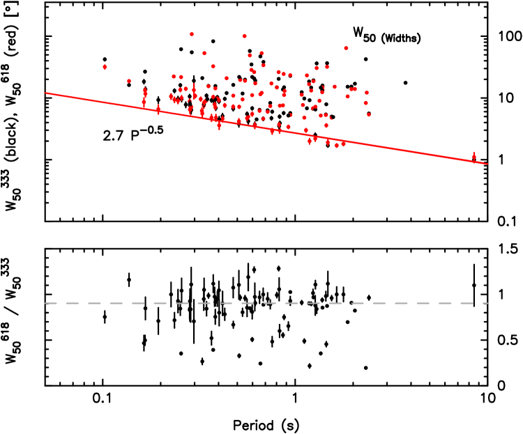
Figure 1: The top panel shows the distribution of widths (measured at outer half-power points) with pulsar period for MSPES sample at 333 and 618 MHz. The points near the LBL consist of both core and cone pulsars and is represented by a guiding line $2.7P^{-0.5}$. The bottom panel show the ratio of widths between 618 and 333 MHz, and a mean value of 0.8 is due to RFM. This figure is reproduced from Fig 2. of Mitra et al. (2016).

In recent works Maciesiak & Gil (2011); Maciesiak et al. (2012) showed that the distribution of half-power width of a large number of pulsars with period could reproduce the LBL. In their sample no distinction was made between any profile class and hence the LBL existed for both core and conal pulsars and were dominated by the lowest angular structures in the average profile. They argued that the LBL is consistent with core and cone emission arising from about 50 stellar radii. The numerical factor $2.45^{\circ}$ was related to the smaller structures in the polar cap and the $P^{-0.5}$ dependence followed from the dipolar nature of the open field lines. As we will discuss below, there is observational evidence that the core and conal emission arises from similar heights of a few hundred kilometers. The finite emission height of core’s would imply that the assumption that core emission arises from last open field lines is invalid.

The presence of the LBL is also seen in the Meter-wavelength Single-Pulse Polametric Emission Survey (MSPES) at 333 and 618 MHz (Mitra et al. 2016), reproduced in Fig.(1). A more detailed study of this data set have revealed that core and cone separately follow the $P^{-0.5}$ scaling relation (Skrzypczak et al. 2017 in preparation). These studies also show that $P^{-0.5}$ scaling is a natural consequence of the dipolar fields only if $\rho^{\nu}$ corresponds to the last open field lines. The components that arise from a certain fixed height and occupy inner regions of the open magnetic field lines do not scale as $P^{-0.5}$. In this case the observed $P^{-0.5}$ dependence must have a different physical origin.

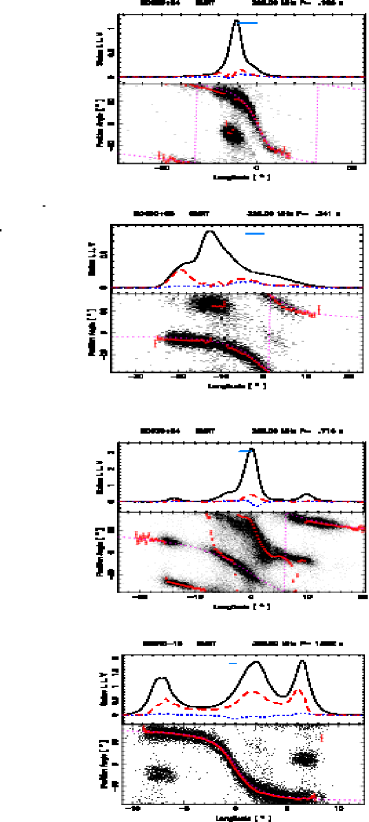
Figure 2: These plots show the application of delay-radius method of finding emission heights given by eq.(6). The plots from top to bottom corresponds to pulsar with increasing period. In each plot the top panel shows the average stokes parameters and the bottom panel shows the polarization histograms. The zero longitude in each plot correspond to the SG point of the PPA and the blue horizontal bar on the top panel shows the delay $\Delta\phi$ The top two plots uses data that was published in Fig.(1) and Fig.(A1) of Mitra & Rankin (2011) and the bottom plot from Fig.(1) of Melikidze et al. (2014).

2.2 Pulse shape and phenomenology

The parameters of the emission beam as well as the line of sight geometry, as discussed above, forms the the basis of the ‘core-cone’ model of emission beam. The pulsar profiles can be broadly classified into the following categories. The central line of sight profiles with three and five components are known as triple (T) amd multiple (M) respectively. More tangential line of sight geometries with one or two components are called conal single (S_d) or conal double D profiles. More detailed discussion on the profile morphology is carried out in Backer (1976); Rankin (1983, 1990, 1993a); Gil et al. (1993); Kijak & Gil (1997). These studies reveal the shape of the pulsar radio emission beam, which can be thought of as an emission pattern projected in the sky, to be composed of a central core emission surrounded by two nested inner and outer cones. Mitra & Deshpande (1999) carried out a multi-frequency analysis and found three nested cones with opening angle given by $\rho^{\nu}=4.8K(1+66\nu^{-1})P^{-0.5}$ where $K=0.8,1,1.2$ for the three cones respectively. They also estimated the angular width of each conal ring to be about 20% of $\rho^{\nu}$. There are studies with contradictory viewpoint about the shape of pulsar emission beam. For example Lyne & Manchester (1988); Han & Manchester (2001) considers the pulsar beam to be composed of random patches with the pulse shape independent of the line of sight geometry. Their conclusions were supported by “partial-cone” pulsars, where the SG point of the PPA was seen at one edge of the profile, giving the impression that part of the emission from the beam was missing. Mitra & Rankin (2011) carried out a detailed single pulse analysis and showed the SG point to lie on the trailing edge of the profile in the “partial-cone” pulsars (see Fig.2). This is indicative of relativistic beaming effect and particularly the presence of single pulse flaring property established the pulse profile shapes to be consistent with the core-cone model. The nested core-cone structure is based on only the MP emission and Basu et al. (2015) showed that the PC components seen in a small sample of pulsars could not be reconciled with the core-cone picture and they likely have different locations within the magnetosphere.

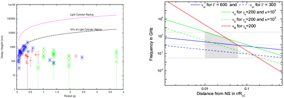
Figure 3: The left panel shows period versus delay-radius emission heights estimated using eq(6) obtained from various sources only for cases where $\Delta\phi$ is positive. The blue points are taken from Table (3) of Weltevrede & Johnston (2008), the green points are obtained from table (3) of Mitra & Li (2004) and red points are obtained from table (A4) of Mitra & Rankin (2011). The right panel plot shows the plasma parameters as a function of the fraction of light cylinder which is reproduced from Fig.(4) of Melikidze et al. (2014, , see text for details).

2.3 Emission Heights

The radio emission height in pulsars is estimated using three different techniques namely the geometrical method, delay-radius method and scintillation studies. The geometrical method gives an estimate of emission height based on eq.(3), which has unresolved issues as discussed in the previous subsection. Rankin (1990, 1993a, 1993b) estimated $h_{em,in,out}^{1GHz}$ to be around 130 and 220 km respectively which were largely independent of the pulsar period. Using a similar approach, but extending the widths to significantly lower thresholds over multiple frequencies, Kijak & Gil (1997) found the height of the outer conal emission to depend mildly on pulsar age and period: $h_{em}\approx 550\nu^{-0.21}\tau_{6}^{-0.1}P^{0.33}$ km, $\tau_{6}$ is characteristic age in $10^{6}$ yr s.

The delay-radius method was suggested by Blaskiewicz et al. (1991, ,hereafter BCW). The method utilizes the fact that the emitting plasma in the co-rotating frame has slightly bent trajectories in the direction of rotation in the observer’s frame. BCW showed that if the emission across the profile originates at a fixed height $h_{em}<<R_{lc}$ (where $R_{lc}=cP/2\pi$ is the light cylinder radius) then the shape of the PPA traverse in eq.(1) is modified such that the phase is shifted by $\Delta\phi\approx 4h_{em}/R_{lc}$ with respect to the center of the pulse profile and the PPA undergoes a downward shift $\Delta\Psi=-(10/3)(h_{em}/R_{lc})\cos(\alpha)$. Hibschman & Arons (2001) (also see Kumar & Gangadhara 2012b, a, 2013), showed that due to polar current $J$ the PPA undergoes a vertical upward shift $\Delta\Psi=(10/3)(h_{em}/R_{lc})J/J_{GJ}\cos(\alpha)$, $J_{GJ}$ is the Goldreich-Julian current density. When $J=J_{GJ}$, $\Delta\Psi$ exactly cancels the shift due to the delay-radius relation. Dyks (2008) provided a lucid physical description of this effect and derived a modified form of eq.(1) in the observer’s frame as:

$$\Psi=\Psi_{\circ}+$$ (5)

$$\tan^{-1}\left(\frac{\sin(\alpha)\sin(\phi-\phi_{f}-2h_{em}/c)}{\sin(\alpha+\beta)\cos(\alpha)-\sin(\alpha)\cos(\alpha+\beta)\cos(\phi-\phi_{f}-2h_{em}/c)}\right)$$

Here $\phi_{f}$ is fiducial pulse phase corresponding to the plane containing the rotation and magnetic axis. If the emission altitude varies significantly across the pulse profile then the PPA traverse can be distorted. However, if emission arises from the same height, $\phi_{f}=(\phi_{c}+\phi_{PPA})/2$, where $\phi_{c}$ is at the center of the pulse profile and $\phi_{PPA}$ is the phase at the SG point. The emission height $h_{em}^{delay}$ is given as

$$h_{em}^{delay}=\frac{c}{4}\frac{\Delta\phi}{360}P~{}~{}~{}{\rm km,}$$ (6)

where $\Delta\phi=(\phi_{PPA}-\phi_{c})$. Estimating the emission height using eq.(6) involves two steps, first is fitting eq.(1) to the PPA traverse to establish a good model for the RVM and obtain an estimate of $\phi_{PPA}$; and secondly to find the midpoint of the profile $\phi_{c}$ by measuring the phase $\phi_{l}$ and $\phi_{t}$ at the leading and trailing edge of the profile such that $\phi_{c}=\phi_{l}+(\phi_{t}-\phi_{l})/2$. The delay-radius method has been used to estimate the emission heights in a large number of pulsars and is around $h_{em}^{delay}\sim 200-500$ km (BCW, von Hoensbroech & Xilouris 1997; Mitra & Li 2004; Mitra & Rankin 2011; Weltevrede & Johnston 2008). Mitra & Li (2004) notes that there are many factors that affect estimates of $h_{em}$ with upto 30% systematic errors. For example, $\phi_{l}$ and $\phi_{t}$ are usually measured at the half-power or 10% level of the profile which might not correspond to the last open field line, or/and the assumption that overall emission arising from the same height might not be correct. In fact for some individual cases $\Delta\phi$ can even be negative, and thus delay-radius height estimates should be used in a statistical sense. It is important to note that eq.(6) has been derived assuming a linear theory with first order terms of $h_{em}/R_{lc}$ retained. Dyks (2008) pointed out that the systematic error due to this approximation is about $(h_{em}/R_{lc})^{0.5}$ and hence for $h_{em}/R_{lc}\sim 0.1$, the error is about 30%. Dyks (2008) also found the theory to be valid for $h_{em}^{delay}/R_{lc}<0.1$ or $\Delta\phi<20^{\circ}$, since second order effects like magnetic field sweep-back, polar currents or Shapiro delay becomes important. Fig.(2) shows the application of the delay-radius method in three pulsars with different periods. In Fig.(3) left panel we show estimates of $h_{em}^{delay}$ from multiple sources (see figure caption) and plot them as a function of period. The heights are roughly constant with period and they lie below 10% of $R_{lc}$. The delay-radius method has also been used to identify the location of the core emission. For example, in the core-dominated pulsar PSR B1933+16 Mitra et al. (2016) both the core and conal emission to be significantly delayed with respect to $\phi_{PPA}$ were shown, thus suggesting similar emission heights for the overall emission. There are a few studies that have used the center of the core emission as the fiducial point (Malov & Suleimanova 1998; Gangadhara & Gupta 2001; Gupta & Gangadhara 2003; Krzeszowski et al. 2009) with the delay-radius relation measuring the conal emission heights with respect to the core component. These studies have suggested that the core emission is emitted slightly lower than the conal emission.

The third method uses the fact that the emission from compact emission region of pulsars traverse through the interstellar medium which act as a varying lens modulating the pulsar signal (Cordes et al. 1983). The extent of modulation depends on the transverse size of the source, and can be estimated using high spatial resolution interferometry. This method has been applied on a small number of pulsars, with accurate results available for the Vela pulsar. The estimated spatial extent of the emission source in Vela pulsar is about 4 km with the corresponding radio emission altitude of about 340 km (see e.g. Johnson et al. 2012).

In summary three independent methods finds the pulsar radio emission altitude $h_{em}\sim 200-500$ km from the neutron star surface. This is a crucial input into theoretical models of pulsar radio emission mechanism.

2.4 Evidence of Curvature radiation

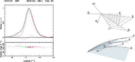
Figure 4: The left panel displays a highly polarized subpulse in a single pulse of PSR B1237+25. The top panel shows the total intensity (black), linear (read dashed) and circular (blue dotted) curves and bottom panel red (for negative circular) and magneta (for positive circular) points show the PPA for the subpulse overlayed on the mean PPA given by gray points. The right hand plot shows the expected change of the electric vector i.e. the PPA across the subpulse for two cases, one for maser emission (upper panel) where the PPA alters quickly across the pulse and second for curvature radiation (lower panel) where the PPA follows the dipolar magnetic field line planes. These plots are reproduced from Fig. 1 and 3 of Mitra et al. (2009).

The RVM is a highly successful model for the PPA even when the PPA appear to be complex and inscrutable. In a majority of such cases the PPA in the single pulses can be separated into two orthogonal polarization modes (OPM) with each of the modal tracks following the RVM, as illustrated in the pulsar B0329+54 (see Fig.2, third panel and also Gil & Lyne 1995; Mitra et al. 2007). The RVM requires both the linearly polarized electric and the dipolar magnetic field line planes from the beamed radiation to change in the same manner across the observers line of sight, making it impossible to fix the relative orientation of the electric polarization with respect to the magnetic field planes using only RVM. There are alternate observing schemes used to determine the orientation of the emerging polarization direction with the most direct evidence based on the X-ray image of the Vela pulsar’s wind nebula (PWN). The high resolution image from the CHANDRA X-ray telescope (Pavlov et al. 2001; Helfand et al. 2001) shows two symmetric arcs coinciding with the direction of the proper motion, $\Psi_{PM}=-53^{\circ}.9\pm 1^{\circ}$. Lai et al. (2001) argued that the arcs are produced by the relativistic pulsar jets flowing out from the neutron star, and the intersection of the arcs coincide with the pulsar rotation axis. The PPA traverse of the Vela pulsar has one single track which is well modelled by the RVM. Lai et al. (2001) used the absolute PPA measurement from Deshpande et al. (1999) and found the SG point to have a value of $\Psi_{\circ}=35\pm 10$. The difference $\mid\Psi_{PM}-\Psi_{\circ}\mid=89^{\circ}\pm 11^{\circ}$, suggests that the the emerging polarization is perpendicular to the magnetic field line planes.

The Vela PWN is the only known case where these studies could be conducted. To circumvent this, other studies have assumed the direction of the proper motion of the pulsar as an indicator of the projection of the rotation axis with the Vela PWN serving as a prototype. In this context Mitra et al. (2007) and Melikidze et al. (2014) investigated PSR B0329+54 and PSR B2045-16 and established that the polarization direction for the two RVM tracks are parallel and perpendicular to the magnetic field line planes. Johnston et al. (2005); Rankin (2007); Noutsos et al. (2012, 2013); Force et al. (2015) estimated a distribution of $\mid\Psi_{PM}-\Psi_{\circ}\mid$ for several pulsars and established a bimodal distribution around 0^∘ and 90^∘. Rankin (2015) found that in core dominated pulsars the distribution is mostly around 90^∘. If we assume the pulsar rotation axis to be along its proper motion, the bi-modality in the distribution can be explained by the presence of OPM, with the emerging radiation either parallel or perpendicular to the magnetic field planes. Alternatively, PMs of pulsars can also be parallel or perpendicular to the rotation axis. While both these explanations are possible, it is evident that the electric vectors of the electromagnetic waves which detach from the pulsar magnetosphere is either parallel or perpendicular to the magnetic field planes.

The implications of the direction of electric polarization are discussed at length in Mitra et al. (2009) and Melikidze et al. (2014). The estimated emission heights $h_{em}$ is the location where the emission escapes from the pulsar magnetosphere. It is possible that the emission is generated in the magnetospheric plasma at a lower height $h_{g}$ ($<h_{em}$). In a hypothetical framework one can imagine the two OPM to be generated at $h_{g}$ in an arbitrary orientation with respect to the magnetic field line planes. In such a scenario an additional mechanism would be required to rotate the polarizations either parallel or perpendicular to magnetic field line planes as they emerge from the plasma at $h_{em}$. Cheng & Ruderman (1979) suggested that adiabatic walking in the region between $h_{g}$ and $h_{em}$ (see Arons & Barnard 1986) can cause any chaotic orientation of the polarization to be rearranged such that they reflect the orthogonal modes in the RVM. However, this does not automatically orient the polarization along parallel or perpendicular to the magnetic plane, which would require additional constraints. The curvature radiation mechanism on the other hand can naturally distinguish the magnetic field line planes. The radiation in the plasma splits into ordinary (O-mode, polarized in the plane of the wave vector ${\bf k}$ and the ${\bf B}$ plane) and the extraordinary (X-mode, polarized perpendicular to the ${\bf k}$ and ${\bf B}$ plane) waves. At emission heights of about 500 km the O-mode can strongly interact with the plasma and emerge as a weaker mode or not emerge at all, while the X-mode can escape the plasma at $h_{g}=h_{em}$ as in vacuum (Melikidze et al., 2014). The power in the O-mode is seven times stronger than the X-mode, and hence in vacuum the O-mode should be the dominant mode of the radiation. The emergence of the X-mode in the Vela pulsar and several other cases provides strong evidence that plasma processes are responsible for the coherent radio emission.

The coherent radio emission from pulsars can be excited by a maser mechanism or via coherent curvature radiation. Mitra et al. (2009) postulated that near 100% linearly polarized single pulses (see Fig.4, left panel) can be used to distinguish between the two emission mechanisms. These highly polarized pulses are not depolarized by the OPMs, and hence carry information of a single polarization mode. They argued that in the case of maser mechanism the k vector can be oriented in any direction with respect to the local magnetic field (see top panel on the right in Fig.4) and the individual subpulses should show PPA swings across mean PPA traverse (modeled by the RVM). On the other hand the waves excited by the coherent curvature radiation are polarized either along the k and local magnetic field plane (O-mode) or perpendicular to the k and magnetic field plane (X-mode). The single pulse observations suggest that pulsar radio emission is excited by coherent curvature radiation which is a definitive solution to the emission mechanism problem.

2.5 Evidence for non-dipolar surface magnetic fields

At heights of 300-500 km from the stellar surface, where the pulsar radio emission originates, the magnetic field is largely dipolar in nature. However, on the neutron star surface the magnetic field should be non-dipolar. The large curvature of the non-dipolar fields are essential for copious pair plasma production which in turn leads to the observed radio emission. The strongest evidence of non-dipolar fields on the surface is provided by the the longest period (8.5 seconds) pulsar J2144$-$3933 (Young et al. 1999). Gil & Mitra (2001) argued that under the polar cap models for this long period significant pair production requires the curvature of the field lines to be $\rho_{c}\sim 10^{5}$ cm. This in turn requires the surface field to be around 10¹⁴ G, which is about 100 times higher than the dipolar magnetic field. Gil et al. (2002) proposed a likely model for surface non-dipolar field which comprises of a global star centered dipole and superposition of local small scale anomalies near the polar cap. Mitra et al. (1999) showed that strong non-dipolar field should not decay significantly over the lifetime of neutron star and Geppert et al. (2013) proposed that crustal hall drift can create such anomalous field structures.

X-ray observations of older pulsars provide estimates of the surface magnetic fields by constraining the size of the polar cap. X-ray emission from neutron star is a mixture of thermal and non-thermal components. The thermal emission can be further separated into two parts, contributions from the whole surface and from the polar cap which acts like a hot spot. In older pulsars the surface temperature cools down below 0.1 millon kelvin whereas the polar cap can be maintained at temperatures larger than a few million kelvin due to bombardment of relativistic back-streaming particles in the acceleration regions above the polar cap. The black-body emission from older pulsars observed in the soft X-rays (0.1 Kev - 10 Kev) can be associated with the hot polar caps. The estimates of the temperature $T_{bb}$, and known distance to the pulsar giving the X-ray luminosity $L_{bb}$ can be used to calculate the area of the polar cap $A_{bb}=L_{bb}/\sigma T_{bb}^{4}$. Comparing the estimated polar cap area with the dipolar polar cap gives a ratio $b=A_{dp}/A_{bb}$, where $A_{dp}=\pi r_{p}^{2}$ and radius $r_{p}=\sqrt{2\pi R_{s}^{3}/cP}$. Invoking conservation of magnetic flux an estimate of the surface magnetic field can be obtained $B_{s}=bB_{d}$.

The above technique has been applied to a number of pulsars to find $b$ (see Becker 2009; table 1.4 from Szary 2013 for a list of pulsars) with specific examples of $A_{bb}<A_{dp}$ are PSR J0108$-$1431 (Pavlov et al. 2009), PSR J0633+1746 (Kargaltsev et al. 2005), PSR B1929+10 (Misanovic et al. 2008), PSR B0943+10 (Mereghetti et al. 2016), PSR B1822-09 (Hermsen et al. 2017), PSR B1133+16 (Szary et al. 2017). In older pulsars $b$ roughly lies in the range $10-500$. It should be noted that the estimates of temperature and area are highly correlated and should be used with caution as evidence of non-dipolar fields. The results are also affected by models of thermal emission that depend on neutron star atmosphere. Several studies (Pavlov & Potekhin, 1995; Zavlin & Pavlov, 2004) show that fits with hydrogen atmospheric models give a lower effective temperature by a factor of 2 and around 10-100 times larger surface areas. Estimates of actual surface area are also complicated by viewing geometry as well as general relativistic effects (Beloborodov, 2002).

In summary the basic inputs to the pulsar emission models from observations are that coherent curvature radio emission is excited in pulsars at a height of about 300$-$500 km above the neutron star surface in regions of open dipolar magnetic field lines and the magnetic field on the neutron star surface are significantly non-dipolar in nature.

3 Plasma condition in the magnetosphere and Mechanism for Radio Emission in Pulsars

The observational results discussed so far are vital inputs into RS75 class of models from the polar cap where the coherent curvature radiation is generated from charged bunches. In this section we will first discuss the basic hypothesis of the RS75 model and the plasma conditions in the magnetosphere. Subsequently, we will discuss the observations which are interpreted based on the polar-cap model.

3.1 Gap Formation:

RS75 suggested that in pulsars where ${\mathbf{\Omega}.B_{s}}<0$ above the magnetic poles, the polar cap is positively charged. Initially there is only a limited supply of positive charges above the polar cap which is relativistically flowing away along the open magnetic field lines as a pulsar wind. If the binding energy of the ions on the neutron star surface are sufficiently large, the region above the polar cap will be charge deficient thereby creating a vacuum gap with large electric fields. They suggested that if a gap of height $h$ exists above the polar cap, the potential drop $\Delta V$ across the gap increases as $h^{2}$ since $\Delta V=\Omega B_{s}h^{2}/c$. Such a gap region can discharge by the generation of electro-positron pairs by photons of energy $>2mc^{2}$. Considering the diffuse background to be the source of such photons the discharge can happen within 100 $\mu$s (Shukre & Radhakrishnan 1982). These charges further accelerate with Lorentz factors $\gamma$ in curved magnetic field lines of radius of curvature $\rho$ to produce high energy curvature radiation photon with frequency $(3/2)\gamma^{3}c/\rho$ which after traveling a mean free path $l_{e}$ can produce another electron-positron pair, such that the gap height $h\sim l_{e}$. To find $h$, RS75 used the Erber (1966) condition where pair creation can happen if the parameter $\chi=(\hbar\omega/2m_{e}c^{2})B_{s}\sin\theta/B_{q}\approx 1/15$. Here the critical magnetic field $B_{q}=m_{e}^{2}c^{3}/e\hbar^{2}=4.4\times 10^{13}$ G and $\theta$ is the angle between the photon and highly curved $B_{s}$ such that $B_{s}\sin\theta\sim B_{s}h/\rho$. In terms of pulsar parameters writing the dipolar component of the field as $B_{d}/10^{12}\sim\sqrt{P\dot{P}_{15}}$ where period derivation $\dot{P_{-15}}=\dot{P}/10^{-15}$s/s and $\rho_{6}=\rho/10^{6}$ cm, $h$ and the maximum potential drop across the gap $\Delta V$ can be expressed as (along with typical values of $b=10$, $P=\rho_{6}=\dot{P}_{15}=1$)

$$h=5\times 10^{3}b^{-4/7}P^{1/7}\dot{P}_{-15}^{-2/7}\rho_{6}^{2/7}\sim 1350\rm{cm}$$ (7)

$$\Delta V=5.2\times 10^{9}b^{-1/7}P^{-3/14}\dot{P}_{-15}^{-1/14}\rho_{6}^{4/7}$$ (8)

$$\sim 3.7\times 10^{9}\rm{[statvolt]}$$

3.2 Spark Formation:

A number of such localized discharge can form in the gap and each such discharge undergoes a pair creation cascade. The electric field in the gap accelerates the electrons towards the stellar surface, while the positrons, often called the primary particles are accelerated away from the surface. At the top of the gap the primary particles acquires Lorentz factors of $\gamma_{p}$ such that

$$\gamma_{p}\approx e\Delta V/m_{e}c^{2}\approx 2\times 10^{6}$$ (9)

As the primary particles move away from the gap region where $\mathbf{E.B}=0$, they continue to create high energy photons, which further create pairs and this cascade leads to the generation of of a cloud of secondary electron-positron plasma which has a significantly lower Lorentz factor with mean value of $\gamma_{s}$. If there are $n_{p}$ primary pairs then the number of secondary pairs can be estimated as $n_{s}\sim(2\gamma_{p}/\gamma_{s})n_{p}$ and thus the density of the secondary plasma increases by a multiplicity factor $\kappa=n_{s}/n_{p}$. The burst of pair-production process increases the charge density along the gap discharge stream and screens the potential in the gap. This process happens exponentially and after a certain time $\tau$ which is estimated to be $\tau\sim 30-40h/c\sim 1\mu$s (RS75), the charge density becomes close to $n_{GJ}$, and the pair-production process stops. During this time the discharge spreads in the lateral direction thus giving a width of $\sim h$ to the discharge. This fully formed discharge is called a “spark” and each spark is associated with a secondary plasma cloud. Once the spark is formed, the spark associated plasma column leaves the gap in a time $\tau_{g}\sim h/c\sim 0.005\mu$s, and as soon as a height $h$ is reached, the next discharge can initiate. Thus in the plasma frame of reference the plasma cloud at a height $h_{em}$ can be thought to be like a cylindrical column of length 30-40$h\sim 1$km along the magnetic axis and having a transverse scale of $h(h_{em}/R_{s})^{0.5}\sim 0.1$ km. lines. The sparking process described above is highly simplistic although numerical simulation of the pair cascade process in one dimension by Timokhin (2010) appears to confirm the non-stationary sparking process. Detailed 3D simulations are required to get a fully consistant theory of spark formation.

3.3 Characteristics of the secondary plasma:

The number density of the secondary plasma cloud is $n_{s}=\kappa n_{GJ}$ since $n_{p}=n_{GJ}$, where $n_{GJ}$ can be expressed in terms of pulsar parameters as

$$n_{GJ}\sim 6\times 10^{10}\left(\frac{\dot{P}_{-15}}{P}\right)^{0.5}\left(\frac{R_{s}}{h_{em}}\right)^{3}\sim~{}~{}5.5\times 10^{5}\rm{cm^{-3}}$$ (10)

with the numerical value obtained for $R_{s}=10$ km and $h_{em}=500$km. Considering radio emission arising at 1 GHz an estimate of $\gamma_{s}\sim(10^{9}\rho 100/c)^{1/3}$ is obtained if one considers curvature radiation from dipolar field lines at $h_{em}=500$ km where $\rho_{6}\sim 100$ cm. This gives $\kappa\sim(n_{p}/n_{s})\sim\gamma_{p}/\gamma_{s}\sim 10^{4}$ (e.g. RS75). The corresponding plasma frequency of the secondary plasma $\omega_{p}^{2}=4\pi e^{2}n_{s}/m_{e}$ is given by

$$\omega_{p}=4.3\times 10^{11}\kappa^{0.5}\left(\frac{\dot{P_{-15}}}{P}\right)^{0.25}\left(\frac{1}{h_{em}}\right)^{1.5}~{}\sim~{}~{}3.7\times 10^{9}\rm{Hz}$$ (11)

The properties of the secondary plasma provides interesting constraints for the radio emission as was discussed by Melikidze et al. (2014) and below we review their arguments. The plasma properties of the secondary plasma can be written in the observer frame of reference in terms of the basic pulsar parameters $P$ (in sec) and ${\dot{P}}$, and as a function of the fractional altitude $\Re=r/R_{\rm LC}$ (here $r$ is the radial distance from the center of the neutron star and $R_{\rm LC}=4.8\times 10^{9}P$ cm is the radius of the light cylinder). The cyclotron frequency $\nu_{B}$ in the local magnetic field $\mathbf{B}$ can be expressed in GHz as,

$$\nu_{B}=\frac{\omega_{B}}{2\pi\gamma_{s}}=5.2\times 10^{-2}\frac{1}{\gamma_{s}}\left(\frac{{\dot{P}_{-15}}}{P^{5}}\right)^{0.5}\Re^{-3}.$$ (12)

The characteristic plasma frequency $\nu_{\circ}$ in GHz can be written as:

$$\nu_{\circ}=\frac{\omega_{0}}{2\pi}=2\times 10^{-5}\kappa^{0.5}\sqrt{\gamma_{s}}\left(\frac{{\dot{P}_{-15}}}{P^{7}}\right)^{0.25}\Re^{-1.5},$$ (13)

where in the observer frame the plasma frequency is $\omega_{\circ}=2\sqrt{\gamma_{s}}\omega_{p}$. As the third parameter we consider the characteristic frequency of the charged solitons (discussed later) coherent curvature radiation, which correspond to the maximum of the power spectrum $\nu_{\rm cr}$ (see Fig. 2 in Gil et al. 2004, GLM04 hereafter),

$$\nu_{\rm cr}=1.2\frac{c{\Gamma}^{3}}{2\pi\rho}=0.8\times 10^{-9}\frac{{\Gamma}^{3}}{P}\Re^{-0.5},$$ (14)

$\Gamma$ is the Lorentz factor of the solitons which is slightly different from $\gamma_{s}$ (see GLM04).

The right panel of Fig. 3 (reproduced from Melikidze et al. (2014))shows $\nu_{B}$ (red line), $\nu_{\circ}$ (green line) and $\nu_{cr}$ (blue line) for a pulsar with $P$= 1 sec and ${\dot{P}}_{-15}$=1, in the observers frame of reference as a function of $\Re$. For the plots a typical value of $\gamma_{s}\sim 200$ is used, and since $\kappa$ has some uncertainty, two extreme value of $\kappa=10^{2}$ and $10^{4}$ has been chosen while plotting $\nu_{\circ}$. Similarly the $\nu_{cr}$ curves are plotted for two extreme values of $\Gamma=300$ and 600. The horizontal gray line correspond to the frequency range of observable radio emission (about 10MHz-10GHz) range and what is noteworthy is that typically $\nu_{cr}<\nu_{\circ}<<\nu_{B}$ for $\Re<0.1$ which is where the radio emission originates (see left panel Fig.(3). The shaded region correspond to the region where two stream instability can grow, which we will discuss in the next section.

3.4 Subpulse drift & $E\times B$ of sparks:

The phenomenon of subpulse drifting discovered by Drake & Craft (1968) is undoubtedly fascinating. In some pulsars, when single pulses are displayed as a pulse stack, where consecutive pulse periods are arranged on top of each other in a two dimensional array with the abscissa as pulse phase and ordinate as pulse longitude, the subpulses in the pulse window are seen to systematically move or drift in pulse phase from one edge to the other edge of the pulse window. Thus an impression of drift bands is seen in the pulse stack where the drifting pattern repeats itself with a frequency $f_{3}$ (or time $P_{3}=1/f_{3}$). The usual technique employed (called longitude resolved fluctuation spectra (LRFS), see Deshpande & Rankin 2001) to recover $f_{3}$ is by performing fast Fourier transforms for every pulse phase within the pulse window along the ordinate axis. Drifting greatly varies in the pulsar population and based on the variation of the phase of the Fourier transform is broadly divided into two groups: phase modulated drifting and amplitude modulated drifting. In the catagory of phase modulated drifting pulsars, where the phase has a positive slope from the leading to the trailing edge, are called negative drifting (ND) while the negative slope cases are called positive drifting (PD). The pulsars where the phase is constant across longitude and only the intensity is modulated, are called amplitude modulated drifting (AMD). Detailed single pulse studies has revealed that the drifting phenomenon in the form of ND, PD or AMD exist for about 45% of the pulsar population (e.g. Weltevrede et al. 2006, Basu et al. 2016).

Drifting is intimately connected with the dynamics of the radio emitting plasma and the sparking model of RS75 is the only successful model that is currently invoked to explain this phenomenon. In the RS75 model, the observed subpulses emitted over a bundle of magnetic open field lines in the dipolar radio emission region ($h_{em}$) can be traced down to the spark associated plasma column in non-dipolar polar cap. The IVG in RS75 model initially has a co-rotational electric field $\mathbf{E_{cor}=-(\Omega\times r)\times B}/c$, and then the gap discharges in the form of multiple sparks. As each spark develops, it initially lags behind co-rotation, and eventually starts to co-rotate when the fully formed spark attains $n_{GJ}$ and the electric field gets entirely screened. During the sparking process, the spark pattern lags behind the co-rotation, although the foot of the sparking location drifts slightly, and hence the new spark initiates at this displaced location. This gives rise to the drifting pattern, and the velocity of the drift motion being $\mathbf{v_{cor}=(E_{cor}\times B)}c/\mathbf{B}^{2}$. RS75 considered an anti-pulsar where the rotation and magnetic axis are aligned but opposite to each other ($\mathbf{\Omega\cdot B=-1}$), and a number of sparks $n_{sp}$ perform drift motion both around the rotation and magnetic axis. Assuming that the sparks perform a circular motion over a time $\hat{P_{3}}=P_{3}n_{sp}$ around the polar cap, RS75 found the expression $\hat{P_{3}}\approx 5.6B_{12}/P^{2}$ in units of $P$. $\hat{P_{3}}$ cannot be easily inferred from observations, but in a detailed analysis of the drifting pulsar PSR B0943+10 Deshpande & Rankin (2001) found evidence of a tertiary periodicity in their LRFS analysis, which they interpreted was due to the spark circulation time $\hat{P_{3}}=37P$, whereas the spark repeating time $P_{3}=1.8P$, gave $n_{s}=20$. To explain this result they proposed the carousel model (which is the anti-pulsar drift model of RS75) for PSR B0943+10 where 20 sparks are circulating around the pulsar magnetic axis and $\hat{P_{3}}$ is the time taken for one spark to return back to the same location. Theoretically the IVG model of RS75 predicts a much smaller value of $\hat{P_{3}}\approx 11P$ for PSR B0943+10, and this led Gil et al. (2004) to introduce partially screened gap (PSG) model where the gap potential is screened by an amount $\eta$ due to presence of ions. The carousel model has also been invoked to explain the nested core-cone structure in pulsar emission. Gil & Sendyk (2000) proposed that the polar cap has a set of circular sparks where the sparks touch each other and the radius of the spark is equal to the gap height $h_{g}$. The central spark remains stationary in phase and correspond to the core emission, while the other sparks rotate around the central spark (like a carousel) to produce the conal emission.

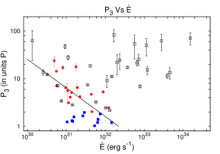
Figure 5: The figure shows the variation of drifting periodicity $P_{3}$ with spin-down energy $\dot{E}$. The red points correspond to PD case, the blue points correspond to ND case and the rest correspond to AMD case. The black line correspond to eq.(15). The figure is reproduced from Fig. (6) of Basu et al. (2016).

Basu et al. (2016) recently pointed out a fundamental difficulty in connecting the carousel model to pulsar data since in a real pulsar the magnetic axis and the rotation axis are not aligned. In such a case the direction of the sparks motion that lag the co-rotation velocity is around the rotation axis and not the magnetic axis. An external observer hence would essentially see that the sparks are drifting across the polar cap. In fact the carousel model for non-aligned pulsar will contradict the basic assumption of the RS75 model as parts of the spark motion in the polar cap will lag the co-rotation velocity while there will be parts that will be leading. For PSR B0943+10 (discussed earlier) invoking a carousel is not essential to interpret $\hat{P_{3}}$. The viewing geometry for this pulsar is highly tangential and the sparks essentially moves along the line of sight, which makes it difficult to infer the path along which the spark moves in the unseen part of the pulsar beam. In the absence of a carousel the periodicity $\hat{P_{3}}$ might have a different physical origin.

In a careful analysis of the MSPES dataset Basu et al. (2016) applied the concept of lagging of sparks to ND and PD pulsars. They argued that $P_{3}=1/f_{3}$ corresponds to the ND cases where sparks lags behind co-rotation, while for PD cases the phase slope appear to be opposite due to aliasing effect and hence $P_{3}=1/(1-f_{3})$. Once this is taken into account a remarkable anti-correlation is seen between $P_{3}$ and the slowdown energy $\dot{E}$ of the pulsar and can be expressed as

$$P_{3}=(\dot{E}/2\times 10^{32})^{-0.6}$$ (15)

This dependence is seen in Fig.(5) where the black line correspond to eq(15). Also note that phase modulation drifting is only seen below $\dot{E}<2\times 10^{32}$ ergs/s, and above this value only phase stationary amplitude modulation is observed. It then appears that the drifting (PD and ND) phenomenon in pulsars can only be observed for $\dot{E}<2\times 10^{32}$ cases. Beyond this value $P_{3}<P$ and hence $P_{3}$ cannot be measured. Thus the AMD cases for $\dot{E}>2\times 10^{32}$ ergs/s might be a entirely new phenomenon as is argued by Basu et al. 2016 and Mitra & Rankin (2017). Under the PSG model the actual drift velocity of sparks is $v_{d}=\eta v_{cor}$, and if one assumes that the polar cap is filled with sparks of size $h$ such that the distance between the sparks is $2h$, then the spark repeating time $P_{3}=2h/v_{d}$. It can be shown the if $\eta$ is small ($\sim 0.1$) then $P_{3}=1/(2\pi\cos(\alpha)\eta)$ (see eq(3.55) Szary 2013) where $\alpha$ is the angle between the rotation and magnetic axis. The factor $\eta\cos(\alpha)\propto\dot{E}^{0.5}$ and hence a dependence of $P_{3}\propto E^{-0.5}$ as see in eq(15) can be obtained (see eq. (12) in Basu et al. (2016). Note that the sparks lags behind co-rotation at the polar cap where the magnetic field is non-dipolar however the spark associated plasma cloud in the emission region is dipolar. Hence the lagging motion of the spark in the polar cap w.r.t the observers line of sight can be very different when it translates to the observed subpulse motion in the emission region at $h_{em}$.

A large number of radio pulsar phenomenon such as pulse microstructure (not discussed here, see e.g. Mitra et al. 2015 for a recent study), shape of pulsar beam, and subpulse drifting, are thought to be related to the sparking process in the IVG. it is important to state that the physics of how the sparks develops in the polar cap is still very unclear, and more insights are necessary to connect theory with observations.

Figure 6: The top panels show the average pulse profile of PSR B0525+21 obtained by folding the interferometric time series data from the Giant Meter-wave Radio Telescope (GMRT) at 325 MHz. The pulse phase regions for the on and off pulse gates are indicated. In the lower panel the contour maps of the on-pulse (bottom left, the on-pulse flux is 21.1$\pm$1.5 mJy) and off-pulse (bottom right, the off-pulse flux is 3.6$\pm$0.3 mJy) emission from the pulsar. The figure is reproduced from Fig. (1) of Basu et al. (2012).

3.5 Off-Pulse Emission, Cyclotron resonance of primary and secondary plasma at outer magnetosphere

In pulsar time series analysis, the off-pulse (OP) region is noise-like without any structure. In certain studies, the search for continuum OP emission has been done by using the technique of gated interferometry. These studies are mostly done to search for radio emission from pulsar wind nebula (PWN) associated with young and energetic pulsars, where the outflowing particles from the pulsar wind can interact with the interstellar medium to produce synchrotron emission observable in the radio band (see e.g. Gaensler et al. 2000). Generally for older pulsars, the energy in the pulsar wind is not sufficient to power a PWN, and hence one does not expect to see any PWN related emission in the OP. A confirmation of this came from the work of Perry & Lyne (1985) where no definite OP emission above 1 mJy was found after performing the search in several older pulsars.

Recently Basu et al. (2011, 2012) conducted a study of OP emission in a number of long period and low energetic pulsars and after doing a very careful analysisi, they surprisingly discovered OP emission at the flux level of a few mJy (see Fig.6). These pulsars however have low slowdown energy hence any emission from the PWN can be ruled out. Further, they demonstrated that the OP emission scintillates in the same manner as the MP and this confirmed that the OP emission has a magnetospheric origin and is coherent in nature. Basu et al. (2013) proposed that the OP emission might be originating in regions close to the light cylinder where the coherent radio OP emission might arise due to growth of cyclotron resonance instability in the outflowing magnetospheric plasma (Kazbegi et al. 1991, Lyutikov 2000). The mechanism can be understood as follows. Since the magnetic field near the light cylinder is weak (a few gauss), the outflowing secondary pair plasma (generated close to the IVG in the polar-cap models) can gyrate around the magnetic field. A large number of electromagnetic modes exists in the plasma, and the transverse X-mode is one such mode which is capable of propagating in the plasma and escape as electromagnetic wave. As the wave propagates, amplification to this wave can be provided by exchange of energy between the wave and fast moving primary plasma particles via the well known cyclotron resonance instability. Basu et al. (2013) derived the growth rate of this instability and determined the magnetospheric OP emission are likely to be detected in pulsars where the dimensionless growth rate $\Gamma\tau>1$, where

$$\Gamma\tau=9.3\left(\frac{P^{3}}{\dot{P}_{15}}\right)$$ (16)

(see eq.(16) of Basu et al. 2013). Note that the MP emission arises from growth of instability in secondary plasma while the OP emission requires interaction between both primary and secondary pair-plasma. Thus, OP emission can be considered as the most direct evidence for the generation of the two component pair-plasma in the pulsar magnetosphere. Application of eq.(16) is currently limited due to lack of sensitive instruments that can detect the low level OP.

4 Growth of Linear Two Stream Instability in Secondary Plasma

In the previous sections we have gathered all evidences that support the polar-cap RS75 kind of model in pulsars. In this section we will discuss the mechanism that excite coherent curvature radiation in pulsars. Recall that in the IVG the non-stationary sparking process can generate flow of successive plasma cloud strictly flowing along a bundle of magnetic dipolar field lines. The non-stationary flow gives rise to situations where slow and fast moving particles can overlap and hence the crucial two-stream instability can develop in the pulsar plasma (RS75, Benford & Buschauer 1977, Egorenkov et al. 1983, Usov 2002 for a review). Each plasma cloud has a mean Lorentz factor $\gamma_{s}$ and there is a sufficient wide spread in $\gamma_{s}$ which arises due to the pair cascade process with typical minimum $\gamma_{min}\sim 10$ and maximum values of $\gamma_{max}\sim 10^{3}-10^{4}$. The overlapping to the slow and fast moving particles of two successive clouds can lead to the two stream instability in plasma. Usov (1987) used simple kinematical estimates to show that this instability can be important for pulsar emission mechanism and that it can develop in the pulsar emission region. Following Melikidze et al. (2000, hereafter MGP00), the typical velocity difference between between the slow and fast moving particles is about $\Delta v=c/(2\gamma_{s}^{2})$, and the typical time for the particles to overlap is $\Delta T=h/\Delta v\sim 2\gamma_{s}^{2}h/c$. Hence, the instability can develop at a distance $r\sim c\Delta T\sim 2\gamma_{s}^{2}h$ which can be written in terms of the pulsar parameter as,

$$r/R\sim 10\left(\frac{\gamma_{s}}{100}\right)^{2}\rho_{6}^{2/7}B_{12}^{-4/7}P^{3/7}$$ (17)

For typical values of parameters $r$ is about a few hundred km which agrees well with the observed emission heights $h_{em}$ derived for pulsars (The instability region is indicated as the shaded region in right panel of Fig.(3)). A significantly detailed study of the two-stream instability considering overlapping of multiple clouds as in the real case was considered by Asseo & Melikidze (1998) and they found instabilities can grow if

$$1.1\times 10^{4}(\gamma_{s}/100)^{-1.5}r^{-1.5}(\dot{P}_{-15}/P)^{0.25}>>0.1$$ (18)

(see eq.(7) of MGP00). This condition can easily develop in the secondary plasma for $\gamma_{s}\sim 100$ and hence the two-stream instability can excite strong electrostatic unstable Langmuir waves, with frequency $\omega_{l}$ which in the observer frame is given by.

$$\omega_{l}=2\delta_{w}{\gamma_{s}}\omega_{p}\approx 4.3\times 10^{11}\kappa^{0.5}\gamma_{s}\left(\frac{\dot{P_{-15}}}{P}\right)^{0.25}\left(\frac{1}{h_{em}}\right)^{0.25}$$ (19)

$$~{}~{}\sim~{}~{}37\times 10^{10}\rm{Hz}$$

where the parameter $\delta_{w}\sim 0.5$ (see Asseo & Melikidze (1998))

5 Coherent Radio emission: Emission From Bunches

Langmuir waves are electrostatic waves, and as they develop in the plasma they tend to bunch the charges with typical length of half the Langmuir wavelength. RS75 and Cheng & Ruderman (1979) suggested that charged bunches formed by linear Langmuir waves can emit coherent curvature radiation near the plasma frequency. This is however impossible as was shown by (Lominadze et al. 1986, MGP00 2000, Melikidze et al. 2014). They argued that curvature radiation with frequency close to the local plasma frequency is impossible, because the coherence condition requires the characteristic dimension of the bunches to be shorter than the wavelength of the radiated wave, which can never be met as the bunch would disperse before the radiation is emitted. Hence high-frequency Langmuir plasma wave cannot be responsible for the coherent pulsar radio-emission (see also Melrose & Gedalin 1999). The other constraint is from observations where the frequency of radio emission is significantly lower than $\omega_{l}$.

Alternatively MGP00 proposed a model for pulsar radio emission based on the modulational instability of Langmuir waves, the basic outcome of the theory is discussed here. MGP00 argued that due to the thermal spread in the plasma the frequency of the Langmuir waves are likely to have a small spread $\Delta\omega$, such that $\Delta\omega<<\omega_{l}$. The amplitude of the Langmuir wave packet will hence be modulated by low-frequency beatings with phase velocity $\Delta\omega/\Delta k$ which is also equal to the group velocity of the plasma wave $v_{g}=d\omega/dk$. Noting that the plasma wave moves in the electron-positron plasma which is also moving relativistically, resonant interactions of plasma particles with low-frequency beatings will lead to modulational instability. Such a process is described by the non-linear Schrödinger equation (NLSE) with non-linear Landau damping. Ichikawa & Taniuti (1973) derived the NLSE taking into account the effect of Landau damping for non relativistic case and applied it to an electron ion plasma. Pataraia & Melikidze (1980) derived the NLSE for the relativistic case and MGP00 applied it to the pulsar system in detail.

Considering the landau damping term to be small they found the corresponding soliton solution by solving the NLSE. In general the Lorentz factors of electrons and positrons in the secondary plasma has slightly different distribution function ($\Delta\gamma=\mid\gamma_{+}-\gamma_{-}\mid$) due to $\Omega.B$ changing along the magnetic field lines (Cheng & Ruderman 1977 , Asseo & Melikidze 1998). If this difference $\Delta\gamma$ is large, then a charge separation can be obtained within the envelope of the soliton (i.e. charged bunches). MPG00 found for reasonable pulsar parameters $\Delta\gamma/\gamma\sim 1$ which was adequate for the various assumptions in the theory like growth of linear instability and derivation of the NLSE to work. The charged solitons thus obtained are supported by pondermotive force (Gaponov & Miller 1958) and are capable of generating coherent curvature radiation. MGP00 found the soliton size $\Delta_{s}\sim 10-100$ cm and coherency of curvature radiation process wavelength of the emitted waves should be longer than the longitudinal size of the soliton $\Delta_{s}$. Thus, the frequencies plotted in Fig. (3) should obey the following constraints $\nu_{cr}<c/\Delta_{s}<\nu_{circ}<<\nu_{B}$ which is clearly the case. The observed pulsar radiation cannot be generated at altitudes exceeding 10% of the light cylinder radius which is consistent with observations. MGP00 showed that in a plasma cloud about 10⁵ solitons can form with each soliton have charge of $Q=e10^{21}$. The power of curvature radiation by a charge $Q$ is $P\approx Q^{2}c\gamma_{s}^{4}/\rho^{2}\sim 10^{25}$ ergs/s, and for a soliton case MGP00 showed that it is 100 times smaller. The incoherent addition of power form the whole soliton cloud multiplied by several number of sparks (say 10) gives the emitter power to be $\sim$10²⁹ ergs/s which can account for the observed radio luminosity in pulsars.

The curvature radiation by solitons excite the transverse X and O mode below $\omega_{\circ}$ which travels with two different speed and the refractive index is such that the X-mode can emerge as in vacuum while the O-mode gets ducted away along the field lines. Melikidze et al. (2014) showed that the difference between the refractive index is constant and hence there is no adiabatic walking of pulsar radiation. There are however two observational effects that still needs to be understood. One effect is the presence of OPM which requires the O-mode to emerge from the plasma, and one suggestion is that gradient in plasma density can cause the O mode to emerge. The second effect is that large amounts of circular polarization are observed, however if the X and O mode separates in phase, the circular polarization is lost, and hence a new mechanism is needed to expalin the circular polarization. Finally, MGP00 ignored the effect of landau-damping while solving the NLSE and hence got stable time-independent soliton solutions. The stability of these solitons needs more investigations.

6 Concluding Remarks

The coherent radio emission from pulsars are intricately linked to the pair creation process around the star. The different plasma parameters are controlled by the pair creation process and sensitive to any stochastic variations. The minimum timescales for any change in the emission process is around 100 milliseconds for a typical pulsar, which is the time taken by the return current to traverse the pulsar magnetosphere. On the other hand a change in the emission state for longer timescales requires additional source of pair creation to alter the nature of the inner acceleration region at longer timescales. The phenomenon of mode changing and nulling in pulsars (not discussed here; see e.g. Basu et al. 2017) where a sudden change in the emission state is observed and persists for longer timescales of varying length is indicative of such changes. Understanding these phenomena requires new physical insights which are outside the purview of the steady state pulsar emission model discussed in this paper.

References

- Arons & Barnard (1986) Arons J., Barnard J. J., 1986, ApJ, 302, 120
- Asseo & Melikidze (1998) Asseo E., Melikidze G. I., 1998, MNRAS, 301, 59
- Backer (1976) Backer D. C., 1976, ApJ, 209, 895
- Basu et al. (2011) Basu R., Athreya R., Mitra D., 2011, ApJ, 728, 157
- Basu et al. (2012) Basu R., Mitra D., Athreya R., 2012, ApJ, 758, 91
- Basu et al. (2013) Basu R., Mitra D., Melikidze G. I., 2013, ApJ, 772, 86
- Basu et al. (2017) Basu R., Mitra D., Melikidze G. I., 2017, ApJ, 846, 109
- Basu et al. (2016) Basu R., Mitra D., Melikidze G. I., Maciesiak K., Skrzypczak A., Szary A., 2016, ApJ, 833, 29
- Basu et al. (2015) Basu R., Mitra D., Rankin J. M., 2015, ApJ, 798, 105
- Becker (2009) Becker W., 2009, in Astrophysics and Space Science Library, Vol. 357, Becker W., ed, Astrophysics and Space Science Library, p. 91
- Beloborodov (2002) Beloborodov A. M., 2002, ApJ, 566, L85
- Benford & Buschauer (1977) Benford G., Buschauer R., 1977, MNRAS, 179, 189
- Blaskiewicz et al. (1991) Blaskiewicz M., Cordes J. M., Wasserman I., 1991, ApJ, 370, 643
- Cheng & Ruderman (1977) Cheng A. F., Ruderman M. A., 1977, ApJ, 212, 800
- Cheng & Ruderman (1979) Cheng A. F., Ruderman M. A., 1979, ApJ, 229, 348
- Cordes et al. (1983) Cordes J. M., Boriakoff V., Weisberg J. M., 1983, ApJ, 268, 370
- Deshpande et al. (1999) Deshpande A. A., Ramachandran R., Radhakrishnan V., 1999, A&A, 351, 195
- Deshpande & Rankin (2001) Deshpande A. A., Rankin J. M., 2001, MNRAS, 322, 438
- Drake & Craft (1968) Drake F. D., Craft H. D., 1968, Nature, 220, 231
- Dyks (2008) Dyks J., 2008, MNRAS, 391, 859
- Dyks & Harding (2004) Dyks J., Harding A. K., 2004, ApJ, 614, 869
- Egorenkov et al. (1983) Egorenkov V. D., Lominadze D. G., Mamradze P. G., 1983, Astrophysics, 19, 426
- Erber (1966) Erber T., 1966, Reviews of Modern Physics, 38, 626
- Everett & Weisberg (2001) Everett J. E., Weisberg J. M., 2001, ApJ, 553, 341
- Force et al. (2015) Force M. M., Demorest P., Rankin J. M., 2015, MNRAS, 453, 4485
- Gaensler et al. (2000) Gaensler B. M., Stappers B. W., Frail D. A., Moffett D. A., Johnston S., Chatterjee S., 2000, MNRAS, 318, 58
- Gangadhara & Gupta (2001) Gangadhara R. T., Gupta Y., 2001, ApJ, 555, 31
- Geppert et al. (2013) Geppert U., Gil J., Melikidze G., 2013, MNRAS, 435, 3262
- Gil et al. (2004) Gil J., Lyubarsky Y., Melikidze G. I., 2004, ApJ, 600, 872
- Gil & Mitra (2001) Gil J., Mitra D., 2001, ApJ, 550, 383
- Gil et al. (1993) Gil J. A., Kijak J., Seiradakis J. H., 1993, A&A, 272, 268
- Gil & Lyne (1995) Gil J. A., Lyne A. G., 1995, MNRAS, 276, L55
- Gil et al. (2002) Gil J. A., Melikidze G. I., Mitra D., 2002, A&A, 388, 235
- Goldreich & Julian (1969) Goldreich P., Julian W. H., 1969, ApJ, 157, 869
- Gupta & Gangadhara (2003) Gupta Y., Gangadhara R. T., 2003, ApJ, 584, 418
- Han & Manchester (2001) Han J. L., Manchester R. N., 2001, MNRAS, 320, L35
- Helfand et al. (2001) Helfand D. J., Gotthelf E. V., Halpern J. P., 2001, ApJ, 556, 380
- Hermsen et al. (2017) Hermsen W. et al., 2017, MNRAS, 466, 1688
- Hibschman & Arons (2001) Hibschman J. A., Arons J., 2001, ApJ, 546, 382
- Ichikawa & Taniuti (1973) Ichikawa Y. H., Taniuti T., 1973, Journal of the Physical Society of Japan, 34, 513
- Johnson et al. (2012) Johnson M. D., Gwinn C. R., Demorest P., 2012, ApJ, 758, 8
- Johnston et al. (2005) Johnston S., Hobbs G., Vigeland S., Kramer M., Weisberg J. M., Lyne A. G., 2005, MNRAS, 364, 1397
- Kargaltsev et al. (2005) Kargaltsev O. Y., Pavlov G. G., Zavlin V. E., Romani R. W., 2005, ApJ, 625, 307
- Kazbegi et al. (1991) Kazbegi A. Z., Machabeli G. Z., Melikidze G. I., 1991, MNRAS, 253, 377
- Kijak & Gil (1997) Kijak J., Gil J., 1997, MNRAS, 288, 631
- Krzeszowski et al. (2009) Krzeszowski K., Mitra D., Gupta Y., Kijak J., Gil J., Acharyya A., 2009, MNRAS, 393, 1617
- Kumar & Gangadhara (2012a) Kumar D., Gangadhara R. T., 2012a, ApJ, 754, 55
- Kumar & Gangadhara (2012b) Kumar D., Gangadhara R. T., 2012b, ApJ, 746, 157
- Kumar & Gangadhara (2013) Kumar D., Gangadhara R. T., 2013, ApJ, 769, 104
- Lai et al. (2001) Lai D., Chernoff D. F., Cordes J. M., 2001, ApJ, 549, 1111
- Lominadze et al. (1986) Lominadze D. G., Machabeli G. Z., Melikidze G. I., Pataraia A. D., 1986, Fizika Plazmy, 12, 1233
- Lyne & Manchester (1988) Lyne A. G., Manchester R. N., 1988, MNRAS, 234, 477
- Lyutikov (2000) Lyutikov M., 2000, MNRAS, 315, 31
- Maciesiak & Gil (2011) Maciesiak K., Gil J., 2011, MNRAS, 417, 1444
- Maciesiak et al. (2012) Maciesiak K., Gil J., Melikidze G., 2012, MNRAS, 424, 1762
- Malov & Suleimanova (1998) Malov I. F., Suleimanova S. A., 1998, Astronomy Reports, 42, 388
- Melikidze et al. (2000) Melikidze G. I., Gil J. A., Pataraya A. D., 2000, ApJ, 544, 1081
- Melikidze et al. (2014) Melikidze G. I., Mitra D., Gil J., 2014, ApJ, 794, 105
- Melrose (1995) Melrose D. B., 1995, Journal of Astrophysics and Astronomy, 16, 137
- Melrose & Gedalin (1999) Melrose D. B., Gedalin M. E., 1999, ApJ, 521, 351
- Mereghetti et al. (2016) Mereghetti S. et al., 2016, ApJ, 831, 21
- Michel & Li (1999) Michel F. C., Li H., 1999, Phys. Rep., 318, 227
- Misanovic et al. (2008) Misanovic Z., Pavlov G. G., Garmire G. P., 2008, ApJ, 685, 1129
- Mitra et al. (2015) Mitra D., Arjunwadkar M., Rankin J. M., 2015, ApJ, 806, 236
- Mitra et al. (2016) Mitra D., Basu R., Maciesiak K., Skrzypczak A., Melikidze G. I., Szary A., Krzeszowski K., 2016, ApJ, 833, 28
- Mitra & Deshpande (1999) Mitra D., Deshpande A. A., 1999, A&A, 346, 906
- Mitra et al. (2009) Mitra D., Gil J., Melikidze G. I., 2009, ApJ, 696, L141
- Mitra et al. (1999) Mitra D., Konar S., Bhattacharya D., 1999, MNRAS, 307, 459
- Mitra & Li (2004) Mitra D., Li X. H., 2004, A&A, 421, 215
- Mitra & Rankin (2017) Mitra D., Rankin J., 2017, ArXiv e-prints
- Mitra et al. (2016) Mitra D., Rankin J., Arjunwadkar M., 2016, MNRAS, 460, 3063
- Mitra & Rankin (2002) Mitra D., Rankin J. M., 2002, ApJ, 577, 322
- Mitra & Rankin (2011) Mitra D., Rankin J. M., 2011, ApJ, 727, 92
- Mitra et al. (2007) Mitra D., Rankin J. M., Gupta Y., 2007, MNRAS, 379, 932
- Noutsos et al. (2012) Noutsos A., Kramer M., Carr P., Johnston S., 2012, MNRAS, 423, 2736
- Noutsos et al. (2013) Noutsos A., Schnitzeler D. H. F. M., Keane E. F., Kramer M., Johnston S., 2013, MNRAS, 430, 2281
- Pataraia & Melikidze (1980) Pataraia A., Melikidze G., 1980, Ap&SS, 68, 61
- Pavlov et al. (2009) Pavlov G. G., Kargaltsev O., Wong J. A., Garmire G. P., 2009, ApJ, 691, 458
- Pavlov & Potekhin (1995) Pavlov G. G., Potekhin A. Y., 1995, ApJ, 450, 883
- Pavlov et al. (2001) Pavlov G. G., Zavlin V. E., Sanwal D., Burwitz V., Garmire G. P., 2001, ApJ, 552, L129
- Perry & Lyne (1985) Perry T. E., Lyne A. G., 1985, MNRAS, 212, 489
- Pétri (2016) Pétri J., 2016, Journal of Plasma Physics, 82, 635820502
- Pétri (2017) Pétri J., 2017, MNRAS, 466, L73
- Radhakrishnan & Cooke (1969) Radhakrishnan V., Cooke D. J., 1969, Astrophys. Lett., 3, 225
- Rankin (1983) Rankin J. M., 1983, ApJ, 274, 333
- Rankin (1990) Rankin J. M., 1990, ApJ, 352, 247
- Rankin (1993a) Rankin J. M., 1993a, ApJ, 405, 285
- Rankin (1993b) Rankin J. M., 1993b, ApJS, 85, 145
- Rankin (2007) Rankin J. M., 2007, ApJ, 664, 443
- Rankin (2015) Rankin J. M., 2015, ApJ, 804, 112
- Ruderman & Sutherland (1975) Ruderman M. A., Sutherland P. G., 1975, ApJ, 196, 51
- Shukre & Radhakrishnan (1982) Shukre C. S., Radhakrishnan V., 1982, ApJ, 258, 121
- Spitkovsky (2011) Spitkovsky A., 2011, Astrophysics and Space Science Proceedings, 21, 139
- Sturrock (1970) Sturrock P. A., 1970, Nature, 227, 465
- Sturrock (1971) Sturrock P. A., 1971, ApJ, 164, 529
- Szary (2013) Szary A., 2013, ArXiv e-prints
- Szary et al. (2017) Szary A., Gil J., Zhang B., Haberl F., Melikidze G. I., Geppert U., Mitra D., Xu R.-X., 2017, ApJ, 835, 178
- Timokhin (2010) Timokhin A. N., 2010, MNRAS, 408, 2092
- Usov (2002) Usov V. V., 2002, in Becker W., Lesch H., Trümper J., ed, Neutron Stars, Pulsars, and Supernova Remnants, p. 240
- von Hoensbroech & Xilouris (1997) von Hoensbroech A., Xilouris K. M., 1997, A&A, 324, 981
- Weltevrede et al. (2006) Weltevrede P., Edwards R. T., Stappers B. W., 2006, A&A, 445, 243
- Weltevrede & Johnston (2008) Weltevrede P., Johnston S., 2008, MNRAS, 391, 1210
- Young et al. (1999) Young M. D., Manchester R. N., Johnston S., 1999, Nature, 400, 848
- Zavlin & Pavlov (2004) Zavlin V. E., Pavlov G. G., 2004, ApJ, 616, 452