Adaptive vertex-centered finite volume methods
for general second-order linear elliptic PDEs

Abstract.

We prove optimal convergence rates for the discretization of a general second-order linear elliptic PDE with an adaptive vertex-centered finite volume scheme. While our prior work Erath and Praetorius [SIAM J. Numer. Anal., 54 (2016), pp. 2228–2255] was restricted to symmetric problems, the present analysis also covers non-symmetric problems and hence the important case of present convection.

1. Introduction

In this work we consider a general second-order linear elliptic PDE and approximate the solution with an adaptive vertex-centered finite volume method (FVM). Finite volume methods are well established in fluid mechanics, since they naturally preserve numerical flux conservation.

1.1. Model problem

Let $\Omega\subset{\mathbb{R}}^{d}$, $d=2,3$, be a bounded Lipschitz domain with polygonal boundary $\Gamma:=\partial\Omega$. As model problem, we consider the following stationary diffusion problem: Given $f\in L^{2}(\Omega)$, find $u\in H^{1}(\Omega)$ such that

(1) $${\rm div}(-\mathbf{A}\nabla u+\mathbf{b}u)+cu =f\quad\text{in }\Omega\qquad\text{and}\qquad u=0\quad\text{on }\Gamma.$$

We suppose that the diffusion matrix $\mathbf{A}=\mathbf{A}(x)\in{\mathbb{R}}^{d\times d}$ is bounded, symmetric, and uniformly positive definite, i.e., there exist constants $\lambda_{\rm min},\lambda_{\rm max}>0$ such that

(2) $$\lambda_{\rm min}\,|\mathbf{v}|^{2}\leq\mathbf{v}^{T}\mathbf{A}(x)\mathbf{v}\leq\lambda_{\rm max}\,|\mathbf{v}|^{2}\quad\text{for all }\mathbf{v}\in{\mathbb{R}}^{d}\text{ and almost all }x\in\Omega.$$

Let ${\mathcal{T}}_{0}$ be a given initial triangulation of $\Omega$; see Section 2.2 below. For convergence of FVM and well-posedness of the residual error estimator, we additionally require that $\mathbf{A}(x)$ is piecewise Lipschitz continuous, i.e.,

(3) $$\mathbf{A}\in W^{1,\infty}(T)^{d\times d}\quad\text{for all }T\in{\mathcal{T}}_{0}.$$

We suppose that the lower-order terms satisfy the assumption

(4) $$\mathbf{b}\in W^{1,\infty}(\Omega)^{d}\text{ and }c\in L^{\infty}(\Omega)\text{ with }\frac{1}{2}{\rm div}\,\mathbf{b}+c\geq 0\text{ almost everywhere on }\Omega.$$

With $(\phi\hskip 1.42262pt,\psi)_{\Omega}=\int_{\Omega}\phi(x)\psi(x)\,dx$ being the $L^{2}$-scalar product, the weak formulation of the model problem Eq. 1 reads as follows: Find $u\in H^{1}_{0}(\Omega)$ such that

(5) $${\mathcal{A}}(u,w):=(\mathbf{A}\nabla u-\mathbf{b}u\hskip 1.42262pt,\nabla w)_{\Omega}+(cu\hskip 1.42262pt,w)_{\Omega}=(f\hskip 1.42262pt,w)_{\Omega}\quad\text{for all }w\in H^{1}_{0}(\Omega).$$

According to our assumptions Eqs. 2 and 4, the bilinear form ${\mathcal{A}}(\cdot,\cdot)$ is continuous and elliptic on $H^{1}_{0}(\Omega)$. Existence and uniqueness of the solution $u\in H^{1}_{0}(\Omega)$ of Eq. 5 thus follow from the Lax-Milgram theorem. Moreover, the operator induced quasi norm $|||\cdot|||$ satisfies that

(6) $$C_{\rm ell}\|v\|_{H^{1}(\Omega)}^{2}\leq|||v|||^{2}:={\mathcal{A}}(v,v)\leq C_{\rm cont}\|v\|_{H^{1}(\Omega)}^{2}\qquad\text{for all }v\in H_{0}^{1}(\Omega),$$

where $C_{\rm ell}>0$ depends only on $\lambda_{\rm min}$ and $\Omega$, whereas $C_{\rm cont}>0$ depends only on $\lambda_{\rm max}$, $\|\mathbf{b}\|_{L^{\infty}(\Omega)}$ and $\|c\|_{L^{\infty}(\Omega)}$.

1.2. Adaptive FVM

In the past 20 years, there have been major contributions to the mathematical understanding of adaptive mesh refinement algorithms, mainly in the context of the finite element method (FEM). While the seminal works [Dör96, MNS00, BDD04, Ste07, CKNS08] were restricted to symmetric operators, the recent works [MN05, CN12, FFP14, BHP17] proved convergence of adaptive FEM with optimal algebraic rates for general second order linear elliptic PDEs. The work [CFPP14] gives an exhausted overview of the developments and it gains, in an abstract framework, a general recipe to prove optimal adaptive convergence rates of adaptive mesh refining algorithms. Basically, the numerical discretization scheme, the a posteriori error estimator and the adaptive algorithm have to fulfill four criteria (called axioms in [CFPP14]), namely, stability on non-refined elements, reduction on refined elements, general quasi-orthogonality, and discrete reliability. Building upon these findings, our recent work [EP16] gave the first proof of convergence of adaptive FVM with optimal algebraic rates for a symmetric model problem Eq. 1 with $\mathbf{b}=0$ and $c=0$.

1.3. Contributions and outline

In this work, we are in particular interested in the non-symmetric model problem with $\mathbf{b}\not=0$ in Eq. 1. The proofs of stability on non-refined elements, reduction on refined elements, and discrete reliability follow basically the proofs in [EP16]; see Section 3.3. Thus, the major contribution of the present work is the proof of the general quasi-orthogonality property for the non-symmetric problem, which is satisfied under some mild regularity assumptions on the dual problem. Similar assumptions are required in [MN05, CN12] to prove convergence for an adaptive FEM procedure. Moreover, we note that [MN05, CN12] require slightly more restrictions on the model data (namely, ${\rm div}(\mathbf{b})=0$) and on the mesh-refinement (the so-called interior node property) for proving quasi-orthogonality which are avoided in the present analysis.

At this point, we note that [FFP14, BHP17] improve the FEM result of [MN05, CN12] by a different approach. Instead of the duality argument, the analysis exploits the a priori convergence of FEM solutions (which follows from the classical Céa lemma) by splitting the operator into a symmetric and elliptic part and a compact perturbation. In particular, there is no duality argument applied and, therefore, no additional regularity assumption is required. However, it seems to be difficult to transfer the analysis of [FFP14, BHP17] to FVM due to the lack of the Céa lemma.

We also mention that unlike the FEM literature, a direct proof of the general quasi-orthogonality is not available for FVM due to the lack of Galerkin orthogonality. Instead, the FVM work [EP16] first proves linear convergence which relies on a quasi-Galerkin orthogonality [EP16, Lemma 11] for FVM. Unfortunately, this auxiliary result does not hold for non-symmetric problems.

Hence, to handle the non-symmetric case, the missing Galerkin orthogonality and the lack of an optimal $L^{2}$ estimate for FVM seem to be the bottlenecks. To overcome these difficulties, we first estimate the FVM error in the bilinear form by oscillations in Lemma 9. Then we provide a new $L^{2}$-type estimate in Lemma 10 which depends on the regularity of the corresponding dual problem plus oscillations. These two results provide the key arguments to prove a quasi-Galerkin orthogonality in Proposition 8. Unlike the literature, this estimate also includes a mesh-size weighted estimator term. With the aid of the previous results, we show linear convergence in Theorem 12, where the proof relies on the previous results. Finally, optimal algebraic convergence rates are guaranteed by Theorem 15 which follows directly from the literature.

We remark that the proposed Algorithm 7 additionally marks oscillations to overcome the lack of classical Galerkin orthogonality. Note that this is not required for adaptive FEM. However, since FVM is not a best approximation method, the proposed approach appears to be rather natural. In practice, however, this additional marking is negligible; see also [EP16, Remark 12]. Overall, the present work seems to be the first which proves convergence with optimal rates of an adaptive FVM algorithm for the solution of general second-order linear elliptic PDEs.

2. Preliminaries

This section introduces the notation, the discrete scheme, as well as the residual a posteriori error estimator. In particular, we fix our notation used throughout this work.

2.1. General notation

Throughout, ${\mathbf{n}}$ denotes the unit normal vector to the boundary pointing outward the respective domain. In the following, we mark the mesh dependency of quantities by appropriate indices, e.g., $u_{\ell}$ is the solution on the triangulation ${\mathcal{T}}_{\ell}$. Furthermore, $\lesssim$ abbreviates $\leq$ up to some (generic) multiplicative constant which is clear from the context.

2.2. Triangulations

The FVM relies on two partitions of $\Omega$, the primal mesh ${\mathcal{T}}_{\times}$ and the associated dual mesh ${\mathcal{T}}_{\times}^{*}$. The primal mesh ${\mathcal{T}}_{\times}$ is a regular triangulation of $\Omega$ into non-degenerate closed triangles/tetrahedra $T\in{\mathcal{T}}_{\times}$, where the possible discontinuities of the coefficient matrix $\mathbf{A}$ are aligned with ${\mathcal{T}}_{\times}$. Define the local mesh-size function

(7) $$h_{\times}\in L^{\infty}(\Omega),\quad h_{\times}|_{T}:=h_{T}:=|T|^{1/d}\quad\text{for all }T\in{\mathcal{T}}_{\times}.$$

Let ${\rm diam}(T)$ be the Euclidean diameter of $T$. Suppose that ${\mathcal{T}}_{\times}$ is $\sigma$-shape regular, i.e.,

(8) $$\max_{T\in{\mathcal{T}}_{\times}}\frac{{\rm diam}(T)}{|T|^{1/d}}\leq\sigma<\infty.$$

Note that this implies $h_{T}\leq{\rm diam}(T)\leq\sigma\,h_{T}$. Let ${\mathcal{N}}_{\times}$ (or ${\mathcal{N}}_{\times}^{\Omega}$) denote the set of all (or all interior) nodes. Let ${\mathcal{F}}_{\times}$ (or ${\mathcal{F}}_{\times}^{\Omega}$) denote the set of all (or all interior) facets. For $T\in{\mathcal{T}}_{\times}$, let ${\mathcal{F}}_{T}:=\big{\{}F\in{\mathcal{F}}_{\times}\,:\,F\subseteq\partial T\big{\}}$ be the set of facets of $T$. Moreover,

(9) $$\omega_{\times}(T):=\bigcup\big{\{}T^{\prime}\in{\mathcal{T}}_{\times}\,:\,T\cap T^{\prime}\neq\emptyset\big{\}}\subseteq\overline{\Omega}$$

denotes the element patch of $T$ in ${\mathcal{T}}_{\times}$.

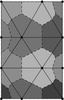
(a) ${\mathcal{T}}_{\times}$ (triangles) and ${\mathcal{T}}_{\times}^{*}$ (grey boxes).

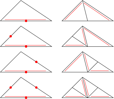
(b) Refinement of a triangle by newest vertex bisection (NVB).

Figure 1. Construction of the dual mesh ${\mathcal{T}}_{\times}^{*}$ from the primal mesh ${\mathcal{T}}_{\times}$ in 2D (left) and 2D newest vertex bisection (right). Each triangle has a reference edge (indicated by the double line). If edges are marked for refinement (indicated by dots), the resulting configurations are shown.

The associated dual mesh ${\mathcal{T}}_{\times}^{*}$ is obtained as follows: For $d=2$, connect the center of gravity of an element $T\in{\mathcal{T}}_{\times}$ with the midpoint of an edge of $\partial T$. These lines define the non-degenerate closed polygons $V_{i}\in{\mathcal{T}}_{\times}^{*}$; see Figure 1(a). For $d=3$, we first connect the center of gravity of $T\in{\mathcal{T}}_{\times}$ with each center of gravity of the four faces of $F\in{\mathcal{F}}_{T}$ by straight lines. Then, as in the 2D case, we connect each center of gravity of $F\in{\mathcal{F}}_{T}$ to the midpoints of the edges of the face $F$. Note that this forms polyhedrons $V_{i}\in{\mathcal{T}}_{\times}^{*}$. In 2D and 3D, each volume $V_{i}\in{\mathcal{T}}_{\times}^{*}$ is uniquely associated with a node $a_{i}$ of ${\mathcal{T}}_{\times}$.

2.3. Discrete spaces

For a partition ${\mathcal{M}}$ of $\Omega$ and $p\in{\mathbb{N}}_{0}$, let

(10) $${\mathcal{P}}^{p}({\mathcal{M}}):=\big{\{}v:\Omega\to{\mathbb{R}}\,:\,\forall M\in{\mathcal{M}}\quad v|_{M}\text{ is polynomial of degree }\leq p\big{\}}$$

be the space of ${\mathcal{M}}$-piecewise polynomials of degree $p$. With this at hand, let

(11) $$\SS^{1}({\mathcal{T}}_{\times}):={\mathcal{P}}^{1}({\mathcal{T}}_{\times})\cap H^{1}(\Omega)=\big{\{}v_{\times}\in C(\Omega)\,:\,\forall T\in{\mathcal{T}}_{\times}\quad v_{\times}|_{T}\text{ is affine}\big{\}}.$$

Then the discrete ansatz space

(12) $$\SS^{1}_{0}({\mathcal{T}}_{\times}):=\SS^{1}({\mathcal{T}}_{\times})\cap H^{1}_{0}(\Omega)=\big{\{}v_{\times}\in\SS^{1}({\mathcal{T}}_{\times})\,:\,v_{\times}|_{\Gamma}=0\big{\}}$$

consists of all ${\mathcal{T}}_{\times}$-piecewise affine and globally continuous functions which are zero on $\Gamma$. By convention, the discrete test space

(13) $${\mathcal{P}}^{0}_{0}({\mathcal{T}}^{*}_{\times}):=\big{\{}v_{\times}^{*}\in{\mathcal{P}}^{0}({\mathcal{T}}_{\times}^{*})\,:\,v_{\times}^{*}|_{\Gamma}=0\big{\}}$$

consists all ${\mathcal{T}}_{\times}^{*}$-piecewise constant functions which are zero on all $V\in{\mathcal{T}}^{*}_{\times}$ with $\partial V\cap\Gamma\not=\emptyset$.

2.4. Mesh-refinements

For local mesh-refinement, we employ newest vertex bisection (NVB); see [Ste08, KPP13] and Figure 1(b). Below, we use the following notation: First, ${\mathcal{T}}^{\prime}:={\tt refine}({\mathcal{T}},{\mathcal{M}})$ denotes the coarsest conforming triangulation generated by NVB from a conforming triangulation ${\mathcal{T}}$ such that all marked elements ${\mathcal{M}}\subseteq{\mathcal{T}}$ have been refined, i.e., ${\mathcal{M}}\subseteq{\mathcal{T}}\backslash{\mathcal{T}}^{\prime}$. Second, we simply write ${\mathcal{T}}^{\prime}\in{\tt refine}({\mathcal{T}})$, if ${\mathcal{T}}^{\prime}$ is an arbitrary refinement of ${\mathcal{T}}$, i.e., there exists a finite number of refinements steps $j=1,\ldots,n$ such that ${\mathcal{T}}^{\prime}={\mathcal{T}}^{\prime}_{n}$ can be generated from ${\mathcal{T}}={\mathcal{T}}^{\prime}_{0}$ with marked elements ${\mathcal{M}}^{\prime}_{j}\subseteq{\mathcal{T}}^{\prime}_{j}$ and ${\mathcal{T}}^{\prime}_{j}={\tt refine}({\mathcal{T}}^{\prime}_{j-1},{\mathcal{M}}^{\prime}_{j-1})$. Note that NVB guarantees that there exist only finitely many shapes of triangles and patches in ${\mathcal{T}}^{\prime}\in{\tt refine}({\mathcal{T}})$. These shapes are determined by ${\mathcal{T}}$. In particular, the meshes ${\mathcal{T}}^{\prime}\in{\tt refine}({\mathcal{T}})$ are uniformly $\sigma$-shape regular Eq. 8, where $\sigma$ depends only on ${\mathcal{T}}$.

2.5. Vertex-centered finite volume method (FVM)

The FVM approximates the solution $u\in H^{1}_{0}(\Omega)$ of Eq. 5 by some $u_{\times}\in\SS^{1}_{0}({\mathcal{T}}_{\times})$. The scheme is based on the balance equation over ${\mathcal{T}}_{\times}^{*}$ and reads in variational form as follows: Find $u_{\times}\in\SS^{1}_{0}({\mathcal{T}}_{\times})$ such that

(14) $${\mathcal{A}}_{\times}(u_{\times},w_{\times}^{*}) =(f\hskip 1.42262pt,w_{\times}^{*})_{\Omega}=\sum_{a_{i}\in{\mathcal{N}}_{\times}^{\Omega}}w_{\times}^{*}|_{V_{i}}\int_{V_{i}}f\,dx\quad\text{for all }w_{\times}^{*}\in{\mathcal{P}}^{0}_{0}({\mathcal{T}}_{\times}^{*}).$$

For all $v_{\times}\in\SS^{1}_{0}({\mathcal{T}}_{\times})$ and all $w_{\times}^{*}\in{\mathcal{P}}^{0}_{0}({\mathcal{T}}_{\times}^{*})$, the bilinear form reads

$${\mathcal{A}}_{\times}(v_{\times},w_{\times}^{*}):=\sum_{a_{i}\in{\mathcal{N}}_{\times}^{\Omega}}w_{\times}^{*}|_{V_{i}}\Big{(}\int_{\partial V_{i}}(-\mathbf{A}\nabla v_{\times}+\mathbf{b}v_{\times})\cdot{\mathbf{n}}\,ds+\int_{V_{i}}cv_{\times}\,dx\Big{)}.$$

To recall that the FVM is well-posed on sufficiently fine triangulations ${\mathcal{T}}_{\times}$, we require the following interpolation operator; see, e.g., [Era12, EP16].

Lemma 1.

With $\chi_{i}^{*}\in{\mathcal{P}}^{0}({\mathcal{T}}_{\times}^{*})$ being the characteristic function of $V_{i}\in{\mathcal{T}}_{\times}^{*}$, define

$${\mathcal{I}}_{\times}^{*}:{\mathcal{C}}(\overline{\Omega})\to{\mathcal{P}}^{0}({\mathcal{T}}^{*}_{\times}),\quad{\mathcal{I}}_{\times}^{*}v:=\sum_{a_{i}\in{\mathcal{N}}_{\times}}v(a_{i})\chi_{i}^{*}.$$

Then, for all $T\in{\mathcal{T}}_{\times}$, $F\in{\mathcal{F}}_{T}$, and $v_{\times}\in\SS^{1}({\mathcal{T}}_{\times})$, it holds that

(15) $$\int_{T}(v_{\times}-{\mathcal{I}}_{\times}^{*}v_{\times})\,dx=0=\int_{F}(v_{\times}-{\mathcal{I}}_{\times}^{*}v_{\times})\,ds,$$

(16) $$\|v_{\times}-{\mathcal{I}}_{\times}^{*}v_{\times}\|_{L^{2}(T)}\leq h_{T}\|\nabla v_{\times}\|_{L^{2}(T)},$$

(17) $$\|v_{\times}-{\mathcal{I}}_{\times}^{*}v_{\times}\|_{L^{2}(F)}\leq Ch_{T}^{1/2}\|\nabla v_{\times}\|_{L^{2}(T)}.$$

In particular, it holds that ${\mathcal{I}}_{\times}^{*}v_{\times}\in{\mathcal{P}}^{0}_{0}({\mathcal{T}}_{\times}^{*})$ for all $v_{\times}\in\SS^{1}_{0}({\mathcal{T}}_{\times})$. The constant $C>0$ depends only on $\sigma$-shape regularity of ${\mathcal{T}}_{\times}$. ∎

The following lemma is a key observation for the FVM analysis. For Lipschitz continuous $\mathbf{A}$, the proof is found in [ELL02, Era12]. We note that the result transfers directly to the present situation [EP16, EP17], where $\mathbf{A}$ satisfies Eq. 2–Eq. 3 and $\mathbf{b}\not=0$ and $c\not=0$.

Lemma 2.

There exists $C_{\rm bil}>0$ such that for all $v_{\times},w_{\times}\in\SS^{1}_{0}({\mathcal{T}}_{\times})$

(18) $$|{\mathcal{A}}(v_{\times},w_{\times})-{\mathcal{A}}_{\times}(v_{\times},{\mathcal{I}}_{\times}^{*}w_{\times})|\leq C_{\rm bil}\sum_{T\in{\mathcal{T}}_{\times}}h_{T}\,\|v_{\times}\|_{H^{1}(T)}\|w_{\times}\|_{H^{1}(T)}.$$

Moreover, let ${\mathcal{T}}_{\times}$ be sufficiently fine such that $C_{\rm ell}-C_{\rm bil}\|h_{\times}\|_{L^{\infty}(\Omega)}>0$, where $C_{\rm ell}>0$ is the ellipticity constant from Eq. 6. Then there exists $C_{\rm stab}>0$ such that

(19) $${\mathcal{A}}_{\times}(v_{\times},{\mathcal{I}}_{\times}^{*}v_{\times})\geq C_{\rm stab}\,\|v_{\times}\|_{H^{1}(\Omega)}^{2}\quad\text{for all }v_{\times}\in\SS^{1}_{0}({\mathcal{T}}_{\times}).$$

In particular, the FVM system Eq. 14 admits a unique solution $u_{\times}\in\SS^{1}_{0}({\mathcal{T}}_{\times})$. The constants $C_{\rm bil}$ and $C_{\rm stab}$ depend only on the data assumptions Eqs. 2 and 4, the $\sigma$-shape regularity of ${\mathcal{T}}_{\times}$, and $\Omega$. ∎

2.6. Weighted-residual a posteriori error estimator

For all $v_{\times}\in\SS^{1}_{0}({\mathcal{T}}_{\times})$, we define the volume residual $R_{\times}$ and the normal jump $J_{\times}$ by

(20) $$R_{\times}(v_{\times})|_{T} :=f-{\rm div}_{\times}(-\mathbf{A}\nabla v_{\times}+\mathbf{b}v_{\times})-cv_{\times}\qquad \text{for all }T\in{\mathcal{T}}_{\times},$$

(21) $$J_{\times}(v_{\times})|_{F} :=[[\mathbf{A}\nabla v_{\times}]]_{F}\qquad \text{for all }F\in{\mathcal{F}}_{\times}^{\Omega}.$$

Here, ${\rm div}_{\times}$ denotes the ${\mathcal{T}}_{\times}$-piecewise divergence operator, and the normal jump reads $[[\mathbf{g}]]|_{F}:=(\mathbf{g}|_{T}-\mathbf{g}|_{T^{\prime}})\cdot{\mathbf{n}}$, where $\mathbf{g}|_{T}$ denotes the trace of $\mathbf{g}$ from $T$ onto $F$ and ${\mathbf{n}}$ points from $T$ to $T^{\prime}$. Let $\Pi_{\times}$ be the edgewise or elementwise integral mean operator, i.e.,

$$(\Pi_{\times})|_{\tau}=\frac{1}{|\tau|}\int_{\tau}v\,dx\qquad\text{for all }\tau\in{\mathcal{T}}_{\times}\cup{\mathcal{F}}_{\times}\text{ and all }v\in L^{2}(\tau).$$

For all $T\in{\mathcal{T}}_{\times}$, we define the local error indicators and oscillations by

(22) $$\begin{split}\eta_{\times}(T,v_{\times})^{2}&:=h_{T}^{2}\,\|R_{\times}(v_{\times})\|_{L^{2}(T)}^{2}+h_{T}\,\|J_{\times}(v_{\times})\|_{L^{2}(\partial T\backslash\Gamma)}^{2},\\ {\rm osc}_{\times}(T,v_{\times})^{2}&:=h_{T}^{2}\,\|(1-\Pi_{\times})R_{\times}(v_{\times})\|_{L^{2}(T)}^{2}+h_{T}\,\|(1-\Pi_{\times})J_{\times}(v_{\times})\|_{L^{2}(\partial T\backslash\Gamma)}^{2}.\end{split}$$

Then the error estimator $\eta_{\times}$ and the oscillations ${\rm osc}_{\times}$ are defined by

(23) $$\eta_{\times}(v_{\times})^{2}:=\sum_{T\in{\mathcal{T}}_{\times}}\eta_{\times}(T,v_{\times})^{2}\qquad\text{and}\qquad{\rm osc}_{\times}^{2}(v_{\times}):=\sum_{T\in{\mathcal{T}}_{\times}}{\rm osc}_{\times}(T,v_{\times})^{2}.$$

To abbreviate notation, we write $\eta_{\times}:=\eta_{\times}(u_{\times})$ and ${\rm osc}_{\times}:={\rm osc}_{\times}(u_{\times})$. The following proposition is proved, e.g., in [CLT05, Era13];

Proposition 3 (reliability and efficiency).

The residual error estimator $\eta_{\times}$ satisfies

(24) $$C_{\rm rel}^{-1}\|u-u_{\times}\|_{H^{1}(\Omega)}^{2}\leq\,\eta_{\times}^{2}\leq\,C_{\rm eff}\big{(}\|u-u_{\times}\|_{H^{1}(\Omega)}^{2}+{\rm osc}_{\times}^{2}),$$

where $C_{\rm rel},C_{\rm eff}>0$ depend only on the $\sigma$-shape regularity of ${\mathcal{T}}_{\times}$, the data assumptions Eqs. 2 and 4, and $\Omega$. ∎

Note that a robust variant of this estimator with respect to an energy norm is found and analyzed in [Era13, Theorem 4.9, Theorem 6.3, and Remark 6.1], where we additionally require the assumption $\|{\rm div}\,\mathbf{b}+c\|_{L^{\infty}(\Omega)}\leq C(\frac{1}{2}{\rm div}\,\mathbf{b}+c)$ with $C>0$. One of the key ingredients of Proposition 3 is Eq. 25 of the following lemma which will be employed below. The proof of the orthogonality relation Eq. 25 is well-known and found, e.g., in [CLT05, Era10, Era13], whereas Eq. 26 is proved in [EP16, Lemma 16] for arbitrary refinement of meshes and can easily be transferred to the present model problem Eq. 1.

Lemma 4.

Let ${\mathcal{T}}_{\diamond}\in{\tt refine}({\mathcal{T}}_{0})$ and ${\mathcal{T}}_{\times}\in{\tt refine}({\mathcal{T}}_{\diamond})$. Suppose that the discrete solutions $u_{\times}\in\SS_{0}^{1}({\mathcal{T}}_{\times})$ or $u_{\diamond}\in\SS_{0}^{1}({\mathcal{T}}_{\times})$ exist. Then there holds the $L^{2}$-orthogonality

(25) $$\sum_{T\in{\mathcal{T}}_{\diamond}}(R_{\diamond}(u_{\diamond})\hskip 1.42262pt,v^{*}_{\diamond})_{T}-\sum_{F\in{\mathcal{F}}_{\diamond}^{\Omega}}(J_{\diamond}(u_{\diamond})\hskip 1.42262pt,v^{*}_{\diamond})_{F} =0\quad\text{for all }v^{*}_{\diamond}\in{\mathcal{P}}^{0}_{0}({\mathcal{T}}^{*}_{\diamond})$$

as well as the discrete defect identity

(26) $$\sum_{T\in{\mathcal{T}}_{\diamond}}(R_{\diamond}(u_{\diamond})\hskip 1.42262pt,v^{*}_{\times})_{T}-\sum_{F\in{\mathcal{F}}_{\diamond}^{\Omega}}(J_{\diamond}(u_{\diamond})\hskip 1.42262pt,v^{*}_{\times})_{F} ={\mathcal{A}}_{\times}(u_{\times}-u_{\diamond},v^{*}_{\times})\text{ for all }v^{*}_{\times}\in{\mathcal{P}}^{0}_{0}({\mathcal{T}}^{*}_{\times}).\qed$$

2.7. Comparison result and a priori error estimate

The following proposition states that the FVM error estimator is equivalent to the optimal total error (i.e., error plus oscillations) and so improves Proposition 3. The result is first proved in [EP16] for $\mathbf{b}=0$ and $c=0$ and generalized to the present model problem in [EP17].

Proposition 5.

Let ${\mathcal{T}}_{\times}$ be sufficiently fine such that $C_{\rm ell}-C_{\rm bil}\|h_{\times}\|_{L^{\infty}(\Omega)}>0$ with $C_{\rm ell}$ and $C_{\rm bil}$ from Eq. 6 and Eq. 18, respectively. Then it holds that

(27) $$\begin{split}C_{1}^{-1}\,\eta_{\times}\leq\min_{v_{\times}\in\SS^{1}_{0}({\mathcal{T}}_{\times})}\big{(}\|u-v_{\times}\|_{H^{1}(\Omega)}+{\rm osc}_{\times}(v_{\times})\big{)}\leq\|u-u_{\times}\|_{H^{1}(\Omega)}+{\rm osc}_{\times}\leq C_{1}\,\eta_{\times}.\end{split}$$

Moreover, if $u_{\times}^{\rm FEM}\in\SS^{1}_{0}({\mathcal{T}}_{\times})$ denotes the FEM solution of ${\mathcal{A}}(u_{\times}^{\rm FEM},w_{\times})=(f,w_{\times})_{\Omega}$ for all $w_{\times}\in\SS^{1}_{0}({\mathcal{T}}_{\times})$, it holds that

$$C_{2}^{-1}\,\big{(}\|u-u_{\times}\|_{H^{1}(\Omega)}+{\rm osc}_{\times}\big{)} \leq\|u-u_{\times}^{\rm FEM}\|_{H^{1}(\Omega)}+{\rm osc}_{\times}(u_{\times}^{\rm FEM})$$

$$\leq C_{2}\,\big{(}\|u-u_{\times}\|_{H^{1}(\Omega)}+{\rm osc}_{\times}\big{)}.$$

The constants $C_{1},C_{2}>0$ depend only on $\Omega$, the $\sigma$-shape regularity of ${\mathcal{T}}_{\times}$, and the data assumptions Eqs. 2 and 4. ∎

As a direct consequence of Proposition 5, one obtains the following convergence result and a priori estimate which confirms first-order convergence of FVM; see again [EP16, EP17]. Note that the statement even holds for $u\in H^{1}_{0}(\Omega)$, whereas in the literature standard FVM analysis usually requires, e.g., $u\in H^{1+\varepsilon}(\Omega)$ for some $\varepsilon>0$.

Corollary 6.

Let $\{{\mathcal{T}}_{\times}\}$ be a family of sufficiently fine and uniformly $\sigma$-shape regular triangulations. Let $u\in H^{1}_{0}(\Omega)$ be the solution of Eq. 5. Then there holds convergence

$$\|u-u_{\times}\|_{H^{1}(\Omega)}+{\rm osc}_{\times}\to 0\quad\text{as}\quad\|h_{\times}\|_{L^{\infty}(\Omega)}\to 0.$$

Moreover, additional regularity $u\in H^{1}_{0}(\Omega)\cap H^{2}(\Omega)$ implies first-order convergence

$$\|u-u_{\times}\|_{H^{1}(\Omega)}+{\rm osc}_{\times}={\mathcal{O}}(\|h_{\times}\|_{L^{\infty}(\Omega)}).\qquad\qed$$

3. Adaptive FVM

In this section, we apply an adaptive mesh-refining algorithm for FVM. We combine ideas from [MN05] and [EP16] to prove that adaptive FVM leads to linear convergence with optimal algebraic rates for the error estimator (and hence for the total error; see Proposition 5).

3.1. Adaptive algorithm

As in [EP16], we employ the following adaptive algorithm:

Algorithm 7.

Input: Let $0<\theta^{\prime}\leq\theta\leq 1$ and $C_{\rm mark},C_{\rm mark}^{\prime}\geq 1$. Let ${\mathcal{T}}_{0}$ be a conforming triangulation of $\Omega$ which resolves possible discontinuities of $\mathbf{A}$.
Loop: For $\ell=0,1,2,\dots$, iterate the following steps (i)–(v):

• Solve: Compute the discrete solution $u_{\ell}\in\SS^{1}_{0}({\mathcal{T}}_{\ell})$ from Eq. 14.

• Estimate: Compute $\eta_{\ell}(T,u_{\ell})$ and ${\rm osc}_{\ell}(T,u_{\ell})$ from Eq. 22 for all $T\in{\mathcal{T}}_{\ell}$.

• Mark I: Find ${\mathcal{M}}_{\ell}^{\eta}\subseteq{\mathcal{T}}_{\ell}$ of up to the multiplicative constant $C_{\rm mark}\geq 1$ minimal cardinality which satisfies the Dörfler marking criterion

  (28) $$\theta\,\sum_{T\in{\mathcal{T}}_{\ell}}\eta_{\ell}(T,u_{\ell})^{2}\leq\sum_{T\in{\mathcal{M}}_{\ell}^{\eta}}\eta_{\ell}(T,u_{\ell})^{2}.$$

• Mark II: Find ${\mathcal{M}}_{\ell}\subseteq{\mathcal{T}}_{\ell}$ of up to the multiplicative constant $C_{\rm mark}^{\prime}\geq 1$ minimal cardinality which satisfies ${\mathcal{M}}_{\ell}^{\eta}\subseteq{\mathcal{M}}_{\ell}$ as well as the Dörfler marking criterion

  (29) $$\theta^{\prime}\,\sum_{T\in{\mathcal{T}}_{\ell}}{\rm osc}_{\ell}(T,u_{\ell})^{2}\leq\sum_{T\in{\mathcal{M}}_{\ell}}{\rm osc}_{\ell}(T,u_{\ell})^{2}.$$

• Refine: Generate new triangulation ${\mathcal{T}}_{\ell+1}:={\tt refine}({\mathcal{T}}_{\ell},{\mathcal{M}}_{\ell})$ by refinement of all marked elements.

Output: Adaptively refined triangulations ${\mathcal{T}}_{\ell}$, corresponding discrete solutions $u_{\ell}$, estimators $\eta_{\ell}$, and data oscillations ${\rm osc}_{\ell}$ for $\ell\geq 0$.

Due to the lack of standard Galerkin orthogonality (see Section 3.2), we additionally have to mark the oscillations Eq. 29. In practice, however, this marking is negligible, since $\theta^{\prime}$ can be chosen arbitrary small; see [EP16, Remark 7] for more details.

3.2. Quasi-Galerkin orthogonality

Given $g\in L^{2}(\Omega)$, we consider the dual problem: Find $\phi\in H^{1}_{0}(\Omega)$ such that

(30) $${\mathcal{A}}(v,\phi)=(g\hskip 1.42262pt,v)_{\Omega}\quad\text{for all }v\in H^{1}_{0}(\Omega).$$

The Lax-Milgram theorem proves existence and uniqueness of $\phi\in H^{1}_{0}(\Omega)$. Let $0<s\leq 1$. We suppose that the dual problem Eq. 30 is $H^{1+s}$-regular, i.e., there exists a constant $C_{\rm dual}>0$ such that for all $g\in L^{2}(\Omega)$, the solution of Eq. 30 satisfies

(31) $$\phi\in H^{1}_{0}(\Omega)\cap H^{1+s}(\Omega)\quad\text{with}\quad\|\phi\|_{H^{1+s}(\Omega)}\leq C_{\rm dual}\,\|g\|_{L^{2}(\Omega)}.$$

We refer to [Gri85] for a discussion on this regularity assumption. The main result of this section is the following quasi-Galerkin orthogonality with respect to the operator-induced quasi norm from Eq. 6. The proof is postponed to the end of this section.

Proposition 8.

Let $0<s\leq 1$ and suppose that the dual problem Eq. 30 is $H^{1+s}$-regular Eq. 31. Let ${\mathcal{T}}_{\diamond}\in{\tt refine}({\mathcal{T}}_{0})$ and ${\mathcal{T}}_{\times}\in{\tt refine}({\mathcal{T}}_{\diamond})$. Then there exists $C_{\rm gal}>0$ such that

(32) $$\begin{split}|||u-u_{\times}|||^{2}&\leq|||u-u_{\diamond}|||^{2}-\frac{1}{2}\,|||u_{\times}-u_{\diamond}|||^{2}+C_{\rm gal}\,\|h_{\times}\|_{L^{\infty}(\Omega)}^{2s}\eta_{\times}^{2}+C_{\rm gal}\,{\rm osc}_{\times}^{2}.\end{split}$$

The constant $C_{\rm gal}>0$ depends only on $C_{\rm dual}$, $C_{\rm osc}$, $C_{\rm rel}$, $C_{\rm ell}$, $C_{\rm cont}$, ${\rm diam}(\Omega)$, and $\|\mathbf{b}\|_{W^{1,\infty}(\Omega)}$ as well as on $\sigma$-shape regularity and all possible shapes of element patches in ${\mathcal{T}}_{\times}$.

For the FVM error, the classical Galerkin orthogonality fails, i.e., ${\mathcal{A}}(u-u_{\times},v_{\times})\not=0$ for some $v_{\times}\in\SS^{1}_{0}({\mathcal{T}}_{\times})$. However, there holds the following estimate; see, e.g., [EP16].

Lemma 9.

The FVM error $u-u_{\times}$ satisfies that

(33) $$|{\mathcal{A}}(u-u_{\times},v_{\times})|\leq C_{\rm osc}\,\|v_{\times}\|_{H^{1}(\Omega)}\,{\rm osc}_{\times}\quad\text{for all }v_{\times}\in\SS^{1}_{0}({\mathcal{T}}_{\times}).$$

The constant $C_{\rm osc}>0$ depends only on $\sigma$-shape regularity of ${\mathcal{T}}_{\times}$.

Proof.

Standard calculations (see, e.g., [Era13, Theorem 4.9]) show that

$${\mathcal{A}}(u-u_{\times},v_{\times}) =\sum_{T\in{\mathcal{T}}_{\times}}\int_{T}R_{\times}(u_{\times})\,v_{\times}\,dx+\sum_{F\in{\mathcal{F}}_{\times}^{\Omega}}\int_{F}J_{\times}(u_{\times})\,v_{\times}\,ds.$$

Together with Eq. 25 for $v^{*}_{\times}={\mathcal{I}}_{\times}^{*}v_{\times}\in{\mathcal{P}}^{0}_{0}({\mathcal{T}}_{\times}^{*})$, this leads to

$${\mathcal{A}}(u-u_{\times},v_{\times})=\sum_{T\in{\mathcal{T}}_{\times}}\int_{T}R_{\times}(u_{\times})\,(v_{\times}-v_{\times}^{*})\,dx+\sum_{F\in{\mathcal{F}}_{\times}^{\Omega}}\int_{F}J_{\times}(u_{\times})\,(v_{\times}-v_{\times}^{*})\,ds.$$

We apply Eq. 15 for the involved integrals and obtain that

$${\mathcal{A}}(u-u_{\times},v_{\times}) =\sum_{T\in{\mathcal{T}}_{\times}}\int_{T}(R_{\times}(u_{\times})-\Pi_{\times}R_{\times}(u_{\times}))\,(v_{\times}-v_{\times}^{*})\,dx$$

$$\qquad+\sum_{F\in{\mathcal{F}}_{\times}^{\Omega}}\int_{F}(J_{\times}(u_{\times})-\Pi_{\times}J_{\times}(u_{\times}))\,(v_{\times}-v_{\times}^{*})\,ds.$$

The Cauchy-Schwarz inequality and Eq. 16–Eq. 17 conclude the proof. ∎

Lemma 10.

Let $0<s\leq 1$ and suppose that the dual problem Eq. 30 is $H^{1+s}$-regular Eq. 31. Then the FVM error satisfies

(34) $$C_{\rm aux}^{-1}\,\|u-u_{\times}\|_{L^{2}(\Omega)}^{2}\leq\|h_{\times}\|_{L^{\infty}(\Omega)}^{2s}\|u-u_{\times}\|_{H^{1}(\Omega)}^{2}+{\rm osc}_{\times}^{2}.$$

The constant $C_{\rm aux}>0$ depends only on the $\sigma$-shape regularity of ${\mathcal{T}}_{\times}$, ${\rm diam}(\Omega)$, $C_{\rm cont}$, and $C_{\rm dual}$ as well as on all possible shapes of element patches in ${\mathcal{T}}_{\times}$.

Proof.

The proof is split into two steps.

Step 1. Let ${\mathcal{I}}_{\times}:H^{1}(\Omega)\to\SS^{1}({\mathcal{T}}_{\times})$ be the Scott-Zhang projector [SZ90]. Recall the following properties of ${\mathcal{I}}_{\times}$ for all $v\in H^{1}(\Omega)$ and $v_{\times}\in\SS^{1}({\mathcal{T}}_{\times})$, and all $T\in{\mathcal{T}}_{\times}$:

• ${\mathcal{I}}_{\times}$ has a local projection property, i.e., $({\mathcal{I}}_{\times}v)|_{T}=v_{\times}|_{T}$ if $v|_{\omega_{\times}(T)}=v_{\times}|_{\omega_{\times}(T)}$;

• ${\mathcal{I}}_{\times}$ preserves discrete boundary data, i.e., $v|_{\Gamma}=v_{\times}|_{\Gamma}$ implies that $({\mathcal{I}}_{\times}v)|_{\Gamma}=v|_{\Gamma}$;

• ${\mathcal{I}}_{\times}$ is locally $H^{1}$-stable, i.e., $\|\nabla{\mathcal{I}}_{\times}v\|_{L^{2}(T)}\leq C_{\rm sz}\,\|\nabla v\|_{H^{1}(\omega_{\times}(T))}$;

• ${\mathcal{I}}_{\times}$ has a local approximation property, i.e., $\|v-{\mathcal{I}}_{\times}v\|_{L^{2}(T)}\leq C_{\rm sz}\,h_{T}\,\|\nabla v\|_{H^{1}(\omega_{\times}(T))}$.

The constant $C_{\rm sz}>0$ depends only on $\sigma$-shape regularity of ${\mathcal{T}}_{\times}$. In particular,

$$\|v-{\mathcal{I}}_{\times}v\|_{H^{1}(\Omega)}\lesssim\|v\|_{H^{1}(\Omega)}\quad\text{for all }v\in H^{1}(\Omega),$$

where the hidden constant depends only on $C_{\rm sz}$ and ${\rm diam}(\Omega)$. With the local projection property of ${\mathcal{I}}_{\times}$, we may apply the Bramble-Hilbert lemma. For $v\in H^{2}(\Omega)$, scaling arguments then prove that

(35) $$\|v-{\mathcal{I}}_{\times}v\|_{H^{1}(T)}\lesssim{\rm diam}(\omega_{\times}(T))\,\|v\|_{H^{2}(\omega_{\times}(T))}\quad\text{for all }T\in{\mathcal{T}}_{\times},$$

where the hidden constant depends only on the shape of $\omega_{\times}(T)$ and on the operator norm of $A:=1-{\mathcal{I}}_{\times}$ (and hence on ${\rm diam}(\Omega)$ and $C_{\rm sz}$). Altogether, this proves the operator norm estimates

(36) $$\|A:=1-{\mathcal{I}}_{\times}:H^{1+t}(\Omega)\to H^{1}(\Omega)\|\leq C\,\|h_{\times}\|_{L^{\infty}(\Omega)}^{t}\quad\text{for }t\in\{0,1\},$$

where $C>0$ depends only on $C_{\rm sz}$, ${\rm diam}(\Omega)$, and all possible shapes of element patches in ${\mathcal{T}}_{\times}$. Interpolation arguments [BL76] conclude that Eq. 36 holds for all $0\leq t\leq 1$. For $t=s$, this proves that

(37) $$\|v-{\mathcal{I}}_{\times}v\|_{H^{1}(\Omega)}\leq C\,\|h_{\times}\|_{L^{\infty}(\Omega)}^{s}\,\|v\|_{H^{1+s}(\Omega)}\quad\text{for all }v\in H^{1+s}(\Omega).$$

Step 2. With $g=v=u-u_{\times}$ in Eq. 30, it holds that

$$\|u-u_{\times}\|_{L^{2}(\Omega)}^{2}={\mathcal{A}}(u-u_{\times},\phi)={\mathcal{A}}(u-u_{\times},\phi-{\mathcal{I}}_{\times}\phi)+{\mathcal{A}}(u-u_{\times},{\mathcal{I}}_{\times}\phi).$$

Since we suppose $\phi\in H^{1+s}(\Omega)$, the first summand is bounded by Eq. 37. This yields that

$${\mathcal{A}}(u-u_{\times},\phi-{\mathcal{I}}_{\times}\phi) \lesssim\|u-u_{\times}\|_{H^{1}(\Omega)}\|\phi-{\mathcal{I}}_{\times}\phi\|_{H^{1}(\Omega)}$$

$$\lesssim\|h_{\times}\|_{L^{\infty}(\Omega)}^{s}\,\|u-u_{\times}\|_{H^{1}(\Omega)}\|\phi\|_{H^{1+s}(\Omega)},$$

where the hidden constants depends only on $C_{\rm cont}$, $C_{\rm sz}$, and ${\rm diam}(\Omega)$. The second summand is bounded by Eq. 33 and $H^{1}$-stability of ${\mathcal{I}}_{\times}$. This yields that

$${\mathcal{A}}(u-u_{\times},{\mathcal{I}}_{\times}\phi)\lesssim{\rm osc}_{\times}\,\|{\mathcal{I}}_{\times}\phi\|_{H^{1}(\Omega)}\lesssim{\rm osc}_{\times}\,\|\phi\|_{H^{1}(\Omega)}\leq{\rm osc}_{\times}\,\|\phi\|_{H^{1+s}(\Omega)},$$

where the hidden constant depends only on $C_{\rm osc}$, $C_{\rm sz}$ and ${\rm diam}(\Omega)$. Combining the latter three estimates with $H^{1+s}$-regularity Eq. 31, we prove that

$$\|u-u_{\times}\|_{L^{2}(\Omega)}^{2} \lesssim\big{(}\|h_{\times}\|_{L^{\infty}(\Omega)}^{s}\,\|u-u_{\times}\|_{H^{1}(\Omega)}+{\rm osc}_{\times}\big{)}\,\|\phi\|_{H^{1+s}(\Omega)}$$

$$\lesssim\big{(}\|h_{\times}\|_{L^{\infty}(\Omega)}^{s}\,\|u-u_{\times}\|_{H^{1}(\Omega)}+{\rm osc}_{\times}\big{)}\,\|u-u_{\times}\|_{L^{2}(\Omega)},$$

where the hidden constant depends additionally on $C_{\rm dual}$. This concludes the proof. ∎

Proof of Proposition 8.

Recall that ${\mathcal{A}}(v,w)=(\mathbf{A}\nabla v\hskip 1.42262pt,\nabla w)_{\Omega}-(\mathbf{b}v\hskip 1.42262pt,\nabla w)_{\Omega}+(cv\hskip 1.42262pt,w)_{\Omega}$ and thus ${\mathcal{A}}(w,v)=(\mathbf{A}\nabla w\hskip 1.42262pt,\nabla v)_{\Omega}-(\mathbf{b}w\hskip 1.42262pt,\nabla v)_{\Omega}+(cw\hskip 1.42262pt,v)_{\Omega}$. For $v,w\in H^{1}_{0}(\Omega)$, integration by parts proves that

$$-(\mathbf{b}w\hskip 1.42262pt,\nabla v)_{\Omega}=(\mathbf{b}\cdot\nabla w\hskip 1.42262pt,v)_{\Omega}+({\rm div}(\mathbf{b})\,w\hskip 1.42262pt,v)_{\Omega}$$

and hence

$${\mathcal{A}}(v,w)+{\mathcal{A}}(w,v)=2{\mathcal{A}}(v,w)+2(v\hskip 1.42262pt,\mathbf{b}\cdot\nabla w)_{\Omega}+({\rm div}(\mathbf{b})\,v\hskip 1.42262pt,w)_{\Omega}.$$

By definition of $|||\cdot|||$, this proves that

$$|||v+w|||^{2} =|||v|||^{2}+|||w|||^{2}+{\mathcal{A}}(v,w)+{\mathcal{A}}(w,v)$$

$$=|||v|||^{2}+|||w|||^{2}+2{\mathcal{A}}(v,w)+2(v\hskip 1.42262pt,\mathbf{b}\cdot\nabla w)_{\Omega}+({\rm div}(\mathbf{b})\,v\hskip 1.42262pt,w)_{\Omega}.$$

This leads to

$$|||v|||^{2}=|||v+w|||^{2}-|||w|||^{2}-2{\mathcal{A}}(v,w)-2(v\hskip 1.42262pt,\mathbf{b}\cdot\nabla w)_{\Omega}-({\rm div}(\mathbf{b})\,v\hskip 1.42262pt,w)_{\Omega}.$$

With $C_{1}:=C_{\rm ell}^{-1}\,(2\|\mathbf{b}\|_{L^{\infty}(\Omega)}+\|{\rm div}(\mathbf{b})\|_{L^{\infty}(\Omega)})^{2}$, the Young inequality $ab\leq\frac{1}{4}\,a^{2}+b^{2}$ and norm equivalence Eq. 6 prove that

$$-2(v\hskip 1.42262pt,\mathbf{b}\cdot\nabla w)_{\Omega}-({\rm div}(\mathbf{b})\,v\hskip 1.42262pt,w)_{\Omega} \leq\|v\|_{L^{2}(\Omega)}\|w\|_{H^{1}(\Omega)}\,\big{(}2\|\mathbf{b}\|_{L^{\infty}(\Omega)}+\|{\rm div}(\mathbf{b})\|_{L^{\infty}(\Omega)}\big{)}$$

$$\leq\frac{1}{4}\,|||w|||^{2}+C_{1}\,\|v\|_{L^{2}(\Omega)}^{2}.$$

Choose $v=u-u_{\times}$ as well as $w=u_{\times}-u_{\diamond}$. So far, we have shown that

$$|||u-u_{\times}|||^{2} \leq|||u-u_{\diamond}|||^{2}-\frac{3}{4}\,|||u_{\times}-u_{\diamond}|||^{2}-2{\mathcal{A}}(u-u_{\times},u_{\times}-u_{\diamond})+C_{1}\,\|u-u_{\times}\|_{L^{2}(\Omega)}^{2}.$$

We apply Eq. 33, norm equivalence Eq. 6, and the Young inequality $2ab\leq\frac{1}{4}\,a^{2}+4b^{2}$ to see that

$$-2{\mathcal{A}}(u-u_{\times},u_{\times}-u_{\diamond})\leq 2\,C_{\rm osc}\,\|u_{\times}-u_{\diamond}\|_{H^{1}(\Omega)}\,{\rm osc}_{\times}$$

$$\qquad\qquad\leq 2\,C_{\rm osc}C_{\rm ell}^{-1/2}\,|||u_{\times}-u_{\diamond}|||\,{\rm osc}_{\times}\leq\frac{1}{4}\,|||u_{\times}-u_{\diamond}|||^{2}+4\,C_{\rm osc}^{2}C_{\rm ell}^{-1}\,{\rm osc}_{\times}^{2}.$$

Next, Lemma 10 and reliability Eq. 24 lead to

$$C_{\rm aux}^{-1}\,\|u-u_{\times}\|_{L^{2}(\Omega)}^{2}\leq\|h_{\times}\|_{L^{\infty}(\Omega)}^{2s}\,\|u-u_{\times}\|_{H^{1}(\Omega)}^{2}+{\rm osc}_{\times}^{2}\leq C_{\rm rel}\,\|h_{\times}\|_{L^{\infty}(\Omega)}^{2s}\,\eta_{\times}^{2}+{\rm osc}_{\times}^{2}.$$

Combining the latter three estimates, we prove that

$$|||u-u_{\times}|||^{2} \leq|||u-u_{\diamond}|||^{2}-\frac{1}{2}\,|||u_{\times}-u_{\diamond}|||^{2}$$

$$\qquad+C_{1}C_{\rm aux}C_{\rm rel}\,\|h_{\times}\|_{L^{\infty}(\Omega)}^{2s}\,\eta_{\times}^{2}+\big{(}4\,C_{\rm osc}^{2}C_{\rm ell}^{-1}+C_{1}C_{\rm aux}\big{)}\,{\rm osc}_{\times}^{2}.$$

Choosing $C_{\rm gal}=\max\{C_{1}C_{\rm aux}C_{\rm rel}\,,\,4C_{\rm osc}^{2}C_{\rm ell}^{-1}+C_{1}C_{\rm aux}\big{\}}$, we conclude the proof. ∎

3.3. Linear convergence and general quasi-orthogonality

The following properties Eqs. A1 and A2 of the estimator and Eqs. B1 and B2 of the oscillations are some key observations to prove linear convergence of Algorithm 7. The proof is based on scaling arguments and can be found in literature, e.g., [CKNS08, Section 3.1] for Eqs. A1 and A2 and [EP16, Section 3.3] for Eqs. B1 and B2. Their proofs apply almost verbatim to the present non-symmetric problem with $\mathbf{b}\not=0$. Therefore, the details are left to the reader.

Lemma 11.

There exist constants $0<q<1$ and $C>0$ such that for all ${\mathcal{T}}_{\diamond}\in{\tt refine}({\mathcal{T}}_{0})$, all ${\mathcal{T}}_{\times}\in{\tt refine}({\mathcal{T}}_{\diamond})$, and all $v_{\times}\in\SS_{0}^{1}({\mathcal{T}}_{\times})$, $v_{\diamond}\in\SS_{0}^{1}({\mathcal{T}}_{\diamond})$, it holds that
(stability of estimator on non-refined elements)

(A1) $$\Big{|}\Big{(}\sum_{T\in{\mathcal{T}}_{\times}\cap{\mathcal{T}}_{\diamond}}\eta_{\times}(T,v_{\times})^{2}\Big{)}^{1/2}-\Big{(}\sum_{T\in{\mathcal{T}}_{\times}\cap{\mathcal{T}}_{\diamond}}\eta_{\diamond}(T,v_{\diamond})^{2}\Big{)}^{1/2}\Big{|}\leq C\,\|v_{\times}-v_{\diamond}\|_{H^{1}(\Omega)},$$

(reduction of estimator on refined elements)

(A2) $$\sum_{T\in{\mathcal{T}}_{\times}\backslash{\mathcal{T}}_{\diamond}}\eta_{\times}(T,v_{\times})^{2}\leq q\sum_{T\in{\mathcal{T}}_{\diamond}\backslash{\mathcal{T}}_{\times}}\eta_{\diamond}(T,v_{\diamond})^{2}+C\,\|v_{\times}-v_{\diamond}\|_{H^{1}(\Omega)}^{2},$$

(stability of oscillations on non-refined elements)

(B1) $$\begin{split}\Big{|}\Big{(}\sum_{T\in{\mathcal{T}}_{\times}\cap{\mathcal{T}}_{\diamond}}{\rm osc}_{\times}(T,v_{\times})^{2}\Big{)}^{1/2}&-\Big{(}\sum_{T\in{\mathcal{T}}_{\times}\cap{\mathcal{T}}_{\diamond}}{\rm osc}_{\diamond}(T,v_{\diamond})^{2}\Big{)}^{1/2}\Big{|}\\ &\leq C\,\|h_{\times}\|_{L^{\infty}(\Omega)}\|v_{\times}-v_{\diamond}\|_{H^{1}(\Omega)},\end{split}$$

(reduction of oscillations on refined elements)

(B2) $$\sum_{T\in{\mathcal{T}}_{\times}\backslash{\mathcal{T}}_{\diamond}}{\rm osc}_{\times}(T,v_{\times})^{2}\leq q\sum_{T\in{\mathcal{T}}_{\diamond}\backslash{\mathcal{T}}_{\times}}{\rm osc}_{\diamond}(T,v_{\diamond})^{2}+C\,\|h_{\times}\|_{L^{\infty}(\Omega)}^{2}\|v_{\times}-v_{\diamond}\|_{H^{1}(\Omega)}^{2}.$$

The constants $0<q<1$ and $C>0$ depend only on the $\sigma$-shape regularity Eq. 8 and on the data assumptions Eqs. 2 and 4.∎

Theorem 12 (linear convergence).

Let $0<\theta^{\prime}\leq\theta\leq 1$. There exists $H>0$ such that the following statement is valid provided that $\|h_{0}\|_{L^{\infty}(\Omega)}\leq H$ and that the dual problem Eq. 30 is $H^{1+s}$-regular Eq. 31 for some $0<s\leq 1$: There exist $C_{\rm lin}>0$ and $0<q_{\rm lin}<1$ such that Algorithm 7 guarantees linear convergence in the sense of

(38) $$\eta_{\ell+n}^{2}\leq C_{\rm lin}q_{\rm lin}^{n}\,\eta_{\ell}^{2}\quad\text{for all }\ell,n\in{\mathbb{N}}_{0}.$$

The constant $H$ depends only on the $\sigma$-shape regularity Eq. 8, on the data assumptions Eqs. 2 and 4, $C_{\rm gal}$, $\theta$, and $\theta^{\prime}$, whereas $C_{\rm lin}$ and $q_{\rm lin}$ additionally depend on $C_{\rm cont}$ and $C_{\rm rel}$.

Proof.

The proof is split into three steps.

Step 1. There exist constants $C>0$ and $0<q<1$ which depend only on $0<\theta\leq 1$, $C_{\rm ell}$, and the constants in Eqs. A1 and A2, such that

(39) $$\eta_{\ell+1}^{2}\leq q\,\eta_{\ell}^{2}+C\,|||u_{\ell+1}-u_{\ell}|||^{2}\quad\text{for all }\ell\in{\mathbb{N}}_{0}.$$

Furthermore, there exist constants $C>0$ and $0<q<1$ which depend only on $0<\theta^{\prime}\leq 1$, $C_{\rm ell}$, and the constants in Eqs. B1 and B2, such that

(40) $${\rm osc}_{\ell+1}^{2}\leq q\,{\rm osc}_{\ell}^{2}+C\,\|h_{\ell+1}\|_{L^{\infty}(\Omega)}^{2}\,|||u_{\ell+1}-u_{\ell}|||^{2}\quad\text{for all }\ell\in{\mathbb{N}}_{0}:$$

The proofs of Eq. 39 and Eq. 40 rely only on Eqs. A1 and A2 with the Dörfler marking Eq. 28 and Eqs. B1 and B2 with marking Eq. 29, respectively. For details, we refer, e.g., to [EP16, Proposition 10 (step 1 and step 2)].

Step 2. Without loss of generality, we may assume that the constants $C>0$ and $0<q<1$ in Eq. 39–Eq. 40 are the same. With free parameters $\gamma,\mu>0$, we define

$$\Delta_{\times}:=|||u-u_{\times}|||^{2}+\gamma\,\eta_{\times}^{2}+\mu\,{\rm osc}_{\times}^{2}.$$

We employ the quasi-Galerkin orthogonality Eq. 32 and obtain that

$$\Delta_{\ell+1}\leq|||u-u_{\ell}|||^{2}+[\gamma+C_{\rm gal}\,\|h_{\ell+1}\|_{L^{\infty}(\Omega)}^{2s}\big{]}\eta_{\ell+1}^{2}+[\mu+C_{\rm gal}]\,{\rm osc}_{\ell+1}^{2}-\frac{1}{2}\,|||u_{\ell+1}-u_{\ell}|||^{2}.$$

Using Eq. 39–Eq. 40, we further derive that

$$\Delta_{\ell+1} \leq|||u-u_{\ell}|||^{2}+\big{[}\gamma+C_{\rm gal}\,\|h_{\ell+1}\|_{L^{\infty}(\Omega)}^{2s}\big{]}\,q\,\eta_{\ell}^{2}+\big{[}\mu+C_{\rm gal}\big{]}\,q\,{\rm osc}_{\ell}^{2}$$

$$\qquad-\bigg{(}\frac{1}{2}-C\,\big{[}\gamma+C_{\rm gal}\,\|h_{\ell+1}\|_{L^{\infty}(\Omega)}^{2s}\big{]}-C\,\|h_{\ell+1}\|_{L^{\infty}(\Omega)}^{2}\,\big{[}\mu+C_{\rm gal}\big{]}\bigg{)}\,|||u_{\ell+1}-u_{\ell}|||^{2}.$$

Let $H>0$ be a free parameter and suppose that $\|h_{0}\|_{L^{\infty}(\Omega)}\leq H$. We estimate $\|h_{\ell+1}\|_{L^{\infty}(\Omega)}\leq\|h_{0}\|_{L^{\infty}(\Omega)}\leq H$. Norm equivalence Eq. 6 and reliability Eq. 24 prove that

$$|||u-u_{\ell}|||^{2}\leq C_{\rm cont}\,\|u-u_{\ell}\|_{H^{1}(\Omega)}^{2}\leq C_{\rm cont}C_{\rm rel}\,\eta_{\ell}^{2}.$$

Let $\varepsilon>0$ be a free parameter. Combining the last two estimates, we see that

$$\Delta_{\ell+1} \leq(1-\varepsilon)\,|||u-u_{\ell}|||^{2}+\gamma\,\big{[}(1+\gamma^{-1}C_{\rm gal}\,H^{2s})q+\gamma^{-1}\varepsilon\,C_{\rm cont}C_{\rm rel}\big{]}\,\eta_{\ell}^{2}+\mu\,\big{[}1+\mu^{-1}C_{\rm gal}\big{]}\,q\,{\rm osc}_{\ell}^{2}$$

$$\qquad-\bigg{(}\frac{1}{2}-C\,\big{[}\gamma+C_{\rm gal}\,H^{2s}\big{]}-C\,H^{2}\big{[}\mu+C_{\rm gal}\big{]}\bigg{)}\,|||u_{\ell+1}-u_{\ell}|||^{2}.$$

Step 3. It only remains to fix the four free parameters $\gamma$, $\mu$, $\varepsilon$, and $H$.

• Choose $\gamma>0$ sufficiently small such that $\gamma C<1/2$.

• Choose $\mu>0$ sufficiently large such that $q_{\rm osc}:=\big{[}1+\mu^{-1}C_{\rm gal}\big{]}\,q<1$.

• Choose $H$ sufficiently small such that

  • $C\,\big{[}\gamma+C_{\rm gal}\,H^{2s}\big{]}+C\,H^{2}\big{[}\mu+C_{\rm gal}\big{]}<1/2$,

  • $(1+\gamma^{-1}C_{\rm gal}\,H^{2s})q<1$.

• Choose $0<\varepsilon<1$ such that $q_{\rm est}:=\big{[}(1+\gamma^{-1}C_{\rm gal}\,H^{2s})q+\gamma^{-1}\varepsilon\,C_{\rm cont}C_{\rm rel}\big{]}<1$.

With $q_{\rm lin}:=\max\{\,1-\varepsilon\,,\,q_{\rm est}\,,\,q_{\rm osc}\,\}$, we then obtain that

$$\Delta_{\ell+1} \leq(1-\varepsilon)\,|||u-u_{\ell}|||^{2}+\gamma\,\big{[}(1+\gamma^{-1}C_{\rm gal}\,H^{2s})q+\gamma^{-1}\varepsilon\,C_{\rm cont}C_{\rm rel}\big{]}\,\eta_{\ell}^{2}+\mu\,\big{[}1+\mu^{-1}C_{\rm gal}\big{]}\,q\,{\rm osc}_{\ell}^{2}$$

$$\leq\max\{\,1-\varepsilon\,,\,q_{\rm est}\,,\,q_{\rm osc}\,\}\,\Delta_{\ell}=q_{\rm lin}\Delta_{\ell}.$$

Induction on $n$, norm equivalence Eq. 6, reliability Eq. 24, and ${\rm osc}_{\ell}^{2}\leq\eta_{\ell}^{2}$ prove that

$$\gamma\,\eta_{\ell+n}^{2}\leq\Delta_{\ell+n}\leq q_{\rm lin}^{n}\Delta_{\ell}\leq q_{\rm lin}^{n}(C_{\rm rel}C_{\rm cont}+\gamma+\mu)\,\eta_{\ell}^{2}\quad\text{for all }\ell,n\in{\mathbb{N}}_{0}$$

This concludes linear convergence Eq. 38 with $C_{\rm lin}=(C_{\rm rel}C_{\rm cont}+\gamma+\mu)\gamma^{-1}$. ∎

From the linear convergence Eq. 38, we immediately obtain the so-called general quasi-orthogonality; see, e.g., [CFPP14, Proposition 4.11] or [EP16, Proposition 10 (step 5)].

Corollary 13 (general quasi-orthogonality).

Let $(u_{k})$ be the sequence of solutions of Algorithm 7. Then there exists $C>0$ such that

(A3) $$\sum_{k=\ell}^{\infty}\|u_{k+1}-u_{k}\|_{H^{1}(\Omega)}^{2}\leq C\,\eta_{\ell}^{2}\quad\text{ for all $\ell\in{\mathbb{N}}_{0}$.}$$

The constant $C>0$ has the same dependencies as $C_{\rm lin}$ from Eq. 38.

3.4. Optimal algebraic convergence rates

In order to prove optimal convergence rates of Algorithm 7, we need one further property of the error estimator, namely the so-called discrete reliability (A4). The proof of the following lemma follows as for the symmetric case in [EP16, Proposition 15]. While the proof is thus omitted, we note that the main difficulties over the well-known FEM proof [CKNS08] arise in the handling of the piecewise constant test space on ${\mathcal{T}}_{\times}^{*}$ and ${\mathcal{T}}_{\diamond}^{*}$, respectively, and the fact that these test spaces are not nested.

Lemma 14 (discrete reliability).

There exists a constant $C>0$ such that for all ${\mathcal{T}}_{\diamond}\in{\tt refine}({\mathcal{T}}_{0})$ and all ${\mathcal{T}}_{\times}\in{\tt refine}({\mathcal{T}}_{\diamond})$, it holds that

(A4) $$\|u_{\times}-u_{\diamond}\|_{H^{1}(\Omega)}^{2}\leq C\Big{(}\sum_{T\in{\mathcal{T}}_{\times}}h_{T}^{2}\|u_{\times}-u_{\diamond}\|_{H^{1}(T)}^{2}+\sum_{T\in{\mathcal{R}}_{\diamond}}\eta_{\diamond}(T,u_{\diamond})^{2}\Big{)},$$

where ${\mathcal{R}}_{\diamond}:=\big{\{}T\in{\mathcal{T}}_{\diamond}\,:\,\exists T^{\prime}\in{\mathcal{T}}_{\diamond}\backslash{\mathcal{T}}_{\times}\text{ with }T\cap T^{\prime}\neq\emptyset\big{\}}$ consists of all refined elements ${\mathcal{T}}_{\diamond}\backslash{\mathcal{T}}_{\times}$ plus one additional layer of neighboring elements. The constant $C>0$ depends only on the $\sigma$-shape regularity Eq. 8, the data assumptions Eqs. 2 and 4, and $\Omega$. Note that for a sufficiently fine initial mesh ${\mathcal{T}}_{0}$, e.g., $C\,\|h_{0}\|_{L^{\infty}(\Omega)}^{2}\leq 1/2$, Eq. A4 leads to discrete reliability as stated in [CFPP14]. ∎

Let ${\mathbb{T}}:={\tt refine}({\mathcal{T}}_{0})$ be the set of all possible triangulations obtained by NVB. For $N\geq 0$, let ${\mathbb{T}}_{N}:=\big{\{}{\mathcal{T}}_{\times}\in{\mathbb{T}}\,:\,\#{\mathcal{T}}_{\times}-\#{\mathcal{T}}_{0}\leq N\big{\}}$. For $s>0$, define

(41) $$\|u\|_{\mathbb{A}_{s}}:=\sup_{N\in{\mathbb{N}}_{0}}\inf_{{\mathcal{T}}_{\times}\in{\mathbb{T}}_{N}}(N+1)^{s}\,\eta_{\times}.$$

Note that $\|u\|_{\mathbb{A}_{s}}<\infty$ implies an algebraic decay $\eta_{\times}={\mathcal{O}}\big{(}(\#{\mathcal{T}}_{\times})^{-s}\big{)}$ along the optimal sequence of meshes (which minimize the error estimator). Optimal convergence of the adaptive algorithm thus means that for all $s>0$ with $\|u\|_{\mathbb{A}_{s}}<\infty$, the adaptive algorithm leads to $\eta_{\ell}={\mathcal{O}}\big{(}(\#{\mathcal{T}}_{\ell})^{-s}\big{)}$. The work [CFPP14, Theorem 4.1] proves in a general framework the following Theorem 15, if the adaptive algorithm applied to a numerical scheme and a corresponding estimator satisfies Eq. A1, Eq. A2, Eq. A3, and Eq. A4.

Theorem 15 (optimal algebraic convergence rates).

Suppose that the dual problem Eq. 30 is $H^{1+s}$-regular Eq. 31 for some $0<s\leq 1$. Let the initial mesh ${\mathcal{T}}_{0}$ be sufficiently fine, i.e, there exists a constant $H>0$ such that $\|h_{0}\|_{L^{\infty}(\Omega)}\leq H$. Finally, suppose that there is a constant $C_{\rm MNS}\geq 1$ such that $\#{\mathcal{M}}_{\ell}\leq C_{\rm MNS}\#{\mathcal{M}}_{\ell}^{\eta}$ for all $\ell\in{\mathbb{N}}_{0}$. Then there exists a bound $0<\theta_{\rm opt}\leq 1$ such that for all $0<\theta<\theta_{\rm opt}$ and all $s>0$ with $\|u\|_{\mathbb{A}_{s}}<\infty$, there exists a constant $C_{\rm opt}>0$ such that

(42) $$\eta_{\ell}\leq C_{\rm opt}(\#{\mathcal{T}}_{\ell}-\#{\mathcal{T}}_{0})^{-s}\quad\text{for all }\ell\in{\mathbb{N}}.$$

The constant $\theta_{\rm opt}$ depends only on $\Omega$, $H$, uniform $\sigma$-shape regularity of the triangulations ${\mathcal{T}}_{\times}\in{\tt refine}({\mathcal{T}}_{0})$, and the data assumptions Eqs. 2 and 4. The constant $C_{\rm opt}$ additionally depends on $s$, the constant $q_{\rm lin}$ from Eq. 38, the use of NVB, and on $C_{\rm MNS}$. ∎

Remark 16.

A direct consequence of the assumption $\#{\mathcal{M}}_{\ell}\leq C_{\rm MNS}\#{\mathcal{M}}_{\ell}^{\eta}$ in Theorem 15 is that data oscillation marking (29) is negligible with respect to the overall number of marked elements [EP16, Remark 7]. In practice, Eq. 28 already implies Eq. 29 since $\theta^{\prime}>0$ can be chosen arbitrarily small. Furthermore, efficiency Eq. 24 is not required to show Eq. 38 and Eq. 42 but guarantees (optimal) linear convergence also for the FVM error.

4. Numerical examples

In extension of our theory, we consider the model problem (1) with inhomogeneous Dirichlet boundary conditions. For all experiments in 2D, we run Algorithm 7 with $\theta=1=\theta^{\prime}$ and $\theta=0.5=\theta^{\prime}$ for uniform mesh-refinement and adaptive mesh-refinement, respectively.

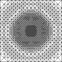
(a) ${\mathcal{T}}_{16}$ (3842 elements).

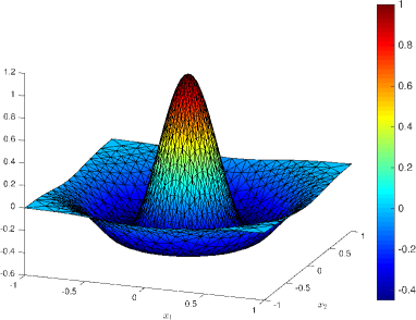
(b) Solution (${\mathcal{T}}_{16}$).

Figure 2. Experiment with smooth solution from Section 4.1: Adaptively generated mesh ${\mathcal{T}}_{16}$ from a uniform initial triangulation ${\mathcal{T}}_{0}$ with $16$ elements, and discrete FVM solution calculated on ${\mathcal{T}}_{16}$.

\psfragscanon\psfrag{s01}[l][l]{\scriptsize$1$}\psfrag{s08}[l][l]{\small$\eta_{\ell}$ (uni.)}\psfrag{s09}[l][l]{\small${\rm osc}_{\ell}$ (ada.)}\psfrag{s10}[l][l]{\scriptsize$1$}\psfrag{s07}[l][l]{\small$E_{\ell}$ (uni.)}\psfrag{s04}[l][l]{\small$\eta_{\ell}$ (ada.)}\psfrag{s02}[l][l]{\small${\rm osc}_{\ell}$ (uni.)}\psfrag{s06}[l][l]{\small$E_{\ell}$ (ada.)}\psfrag{s03}[l][l]{\scriptsize$\;\;\;\;\;\;\;\;1$}\psfrag{s14}[l][l]{\scriptsize$\;\;\;1/2$}\psfrag{s05}[t][t]{\small number of elements}\psfrag{s11}[b][b]{\small error, estimator, oscillation}\psfrag{x01}[t][t]{\scriptsize${10^{1}}$}\psfrag{x02}[t][t]{\scriptsize${10^{2}}$}\psfrag{x03}[t][t]{\scriptsize${10^{3}}$}\psfrag{x04}[t][t]{\scriptsize${10^{4}}$}\psfrag{x05}[t][t]{\scriptsize${10^{5}}$}\psfrag{x06}[t][t]{\scriptsize${10^{6}}$}\psfrag{x07}[t][t]{\scriptsize${10^{7}}$}\psfrag{v01}[r][r]{\scriptsize${10^{-3}}$}\psfrag{v02}[r][r]{\scriptsize${10^{-2}}$}\psfrag{v03}[r][r]{\scriptsize${10^{-1}}$}\psfrag{v04}[r][r]{\scriptsize${10^{0}}$}\psfrag{v05}[r][r]{\scriptsize${10^{1}}$}\psfrag{v06}[r][r]{\scriptsize${10^{2}}$}\psfrag{v07}[r][r]{\scriptsize${10^{3}}$}\includegraphics[width=346.89731pt]{figures/bsp1-error.eps}

Figure 3. Experiment with smooth solution from Section 4.1: Error $E_{\ell}=\|u-u_{\ell}\|_{H^{1}(\Omega)}$, weighted-residual error estimator $\eta_{\ell}$, and data oscillations ${\rm osc}_{\ell}$ for uniform and adaptive mesh-refinement.

4.1. Experiment with smooth solution

On the square $\Omega=(-1,1)^{2}$, we prescribe the exact solution $u(x_{1},x_{2})=(1-10x_{1}^{2}-10x_{2}^{2})e^{-5(x_{1}^{2}+x_{2}^{2})}$ with $x=(x_{1},x_{2})\in{\mathbb{R}}^{2}$. We choose the diffusion matrix

$$\mathbf{A}=\left(\begin{array}[]{rr}10+\cos x_{1}&9\,x_{1}x_{2}\\ 9\,x_{1}x_{2}&\;10+\sin x_{2}\end{array}\right),$$

the velocity $\mathbf{b}=(\sin x_{1},\cos x_{2})^{T}$ and the reaction $c=1$. Note that Eq. 2 holds with $\lambda_{\min}=0.82293$ and $\lambda_{\max}=10.84096$, and Eq. 4 with $\frac{1}{2}{\rm div}\mathbf{b}+c>0$. The right-hand side $f$ is calculated appropriately. The uniform initial mesh ${\mathcal{T}}_{0}$ consists of the $16$ triangles.

In Figure 22(a) we see an adaptively generated mesh after $16$ refinements. Figure 22(b) plots the smooth solution on the mesh ${\mathcal{T}}_{16}$. Both, uniform and adaptive mesh-refinement, lead to the optimal convergence order ${\mathcal{O}}(N^{-1/2})$ with respect to the number $N$ of elements since $u$ is smooth; see Figure 3. The oscillations are of higher order and decrease with ${\mathcal{O}}(N^{-1})$.

Table 1 shows the experimental validation of the additional assumption in Theorem 15, i.e., marking for the data oscillations is negligible; see also Remark 16.

$\ell$	$\#{\mathcal{T}}_{\ell}$	$\frac{\#{\mathcal{M}}_{\ell}}{\#{\mathcal{M}}_{\ell}^{\eta}}$	$\frac{{\rm osc}_{\ell}({\mathcal{M}}_{\ell}^{\eta})^{2}}{{\rm osc}_{\ell}^{2}}$
0	16	1.000	0.631
1	22	1.000	0.615
2	28	1.000	0.704
3	32	1.000	0.769
4	40	1.214	0.338
5	78	1.111	0.446
6	112	1.133	0.292
7	156	1.119	0.410
8	216	1.062	0.394
9	331	1.198	0.264
10	460	1.014	0.472
11	660	1.049	0.371

$\ell$	$\#{\mathcal{T}}_{\ell}$	$\frac{\#{\mathcal{M}}_{\ell}}{\#{\mathcal{M}}_{\ell}^{\eta}}$	$\frac{{\rm osc}_{\ell}({\mathcal{M}}_{\ell}^{\eta})^{2}}{{\rm osc}_{\ell}^{2}}$
12	944	1.027	0.431
13	1,338	1.025	0.400
14	1,910	1.018	0.387
15	2,748	1.026	0.374
16	3,842	1.015	0.358
17	5,430	1.003	0.449
18	7,438	1.013	0.359
19	10,590	1.003	0.445
20	14,478	1.019	0.323
21	20,286	1.004	0.430
22	27,558	1.004	0.457
23	38,450	1.010	0.324

$\ell$	$\#{\mathcal{T}}_{\ell}$	$\frac{\#{\mathcal{M}}_{\ell}}{\#{\mathcal{M}}_{\ell}^{\eta}}$	$\frac{{\rm osc}_{\ell}({\mathcal{M}}_{\ell}^{\eta})^{2}}{{\rm osc}_{\ell}^{2}}$
24	52,422	1.000	0.540
25	72,454	1.007	0.404
26	98,232	1.000	0.508
27	135,172	1.004	0.446
28	184,142	1.000	0.606
29	251,896	1.002	0.475
30	342,148	1.001	0.488
31	461,674	1.000	0.617
32	635,266	1.004	0.416
33	852,730	1.000	0.664
34	1,172,122	1.002	0.464

Table 1. Experiment with smooth solution from Section 4.1: We compute $\widetilde{C}_{MNS}:=\#{\mathcal{M}}_{\ell}/\#{\mathcal{M}}_{\ell}^{\eta}\leq 1.3$. Hence, the additional assumption in Theorem 15 is experimentally verified. Furthermore, we compute $\widetilde{\theta}^{\prime}:={\rm osc}_{\ell}({\mathcal{M}}_{\ell}^{\eta})^{2}/{\rm osc}_{\ell}^{2}\geq 0.2$ with ${\rm osc}_{\ell}({\mathcal{M}}_{\ell}^{\eta})^{2}:=\sum_{T\in{\mathcal{M}}_{\ell}^{\eta}}{\rm osc}_{\ell}(T,u_{\ell})^{2}$, i.e., the choice $\theta=0.5$, $\theta^{\prime}=0.2$ would guarantee ${\mathcal{M}}_{\ell}={\mathcal{M}}_{\ell}^{\eta}$ in Algorithm 7.

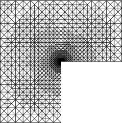
(a) ${\mathcal{T}}_{16}$ (2534 elements).

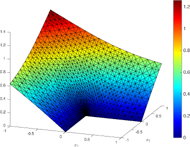
(b) Solution (${\mathcal{T}}_{16}$).

Figure 4. Experiment with generic singularity in the reentrant corner $(0,0)$ from Section 4.2: Adaptively generated mesh ${\mathcal{T}}_{16}$ from a uniform initial triangulation ${\mathcal{T}}_{0}$ with $12$ elements, and discrete FVM solution calculated on ${\mathcal{T}}_{16}$.

\psfragscanon\psfrag{s08}[l][l]{\small${\rm osc}_{\ell}$ (uni.)}\psfrag{s15}[t][t]{\small number of elements}\psfrag{s05}[l][l]{\small$E_{\ell}$ (uni.)}\psfrag{s16}[l][l]{\small$\eta_{\ell}$ (uni.)}\psfrag{s12}[l][l]{\small$E_{\ell}$ (ada.)}\psfrag{s13}[b][b]{\small error, estimator, oscillation}\psfrag{s10}[l][l]{\scriptsize$\;\;\;\;\;\;\;\;\;\;1/2$}\psfrag{s14}[l][l]{\small${\rm osc}_{\ell}$ (ada.)}\psfrag{s02}[l][l]{\scriptsize$1$}\psfrag{s03}[l][l]{\scriptsize$\;\;\;\;\;\;\;\;\;\;1$}\psfrag{s04}[l][l]{\scriptsize$\;\;\;1/3$}\psfrag{s09}[l][l]{\small$\eta_{\ell}$ (ada.)}\psfrag{s06}[l][l]{\scriptsize$1$}\psfrag{s07}[l][l]{\scriptsize$1$}\psfrag{x01}[t][t]{\scriptsize${10^{1}}$}\psfrag{x02}[t][t]{\scriptsize${10^{2}}$}\psfrag{x03}[t][t]{\scriptsize${10^{3}}$}\psfrag{x04}[t][t]{\scriptsize${10^{4}}$}\psfrag{x05}[t][t]{\scriptsize${10^{5}}$}\psfrag{x06}[t][t]{\scriptsize${10^{6}}$}\psfrag{x07}[t][t]{\scriptsize${10^{7}}$}\psfrag{v01}[r][r]{\scriptsize${10^{-5}}$}\psfrag{v02}[r][r]{\scriptsize${10^{-4}}$}\psfrag{v03}[r][r]{\scriptsize${10^{-3}}$}\psfrag{v04}[r][r]{\scriptsize${10^{-2}}$}\psfrag{v05}[r][r]{\scriptsize${10^{-1}}$}\psfrag{v06}[r][r]{\scriptsize${10^{0}}$}\psfrag{v07}[r][r]{\scriptsize${10^{1}}$}\includegraphics[width=346.89731pt]{figures/bsp2-error.eps}

Figure 5. Experiment with generic singularity from Section 4.2: Error $E_{\ell}=\|u-u_{\ell}\|_{H^{1}(\Omega)}$, weighted-residual error estimator $\eta_{\ell}$, and data oscillations ${\rm osc}_{\ell}$ for uniform and adaptive mesh-refinement.

$\ell$	$\#{\mathcal{T}}_{\ell}$	$\frac{\#{\mathcal{M}}_{\ell}}{\#{\mathcal{M}}_{\ell}^{\eta}}$	$\frac{{\rm osc}_{\ell}({\mathcal{M}}_{\ell}^{\eta})^{2}}{{\rm osc}_{\ell}^{2}}$
0	12	1.667	0.135
1	18	1.750	0.086
2	29	1.600	0.027
3	40	1.375	0.057
4	56	1.400	0.252
5	74	1.667	0.079
6	114	1.286	0.148
7	153	1.188	0.243
8	212	1.111	0.256
9	284	1.065	0.390
10	380	1.194	0.168
11	539	1.068	0.328

$\ell$	$\#{\mathcal{T}}_{\ell}$	$\frac{\#{\mathcal{M}}_{\ell}}{\#{\mathcal{M}}_{\ell}^{\eta}}$	$\frac{{\rm osc}_{\ell}({\mathcal{M}}_{\ell}^{\eta})^{2}}{{\rm osc}_{\ell}^{2}}$
12	721	1.050	0.346
13	991	1.007	0.466
14	1,356	1.003	0.482
15	1,852	1.020	0.386
16	2,534	1.000	0.630
17	3,413	1.009	0.443
18	4,684	1.000	0.597
19	6,341	1.003	0.443
20	8,568	1.002	0.490
21	11,564	1.000	0.640
22	15,590	1.000	0.539
23	21,071	1.000	0.569

$\ell$	$\#{\mathcal{T}}_{\ell}$	$\frac{\#{\mathcal{M}}_{\ell}}{\#{\mathcal{M}}_{\ell}^{\eta}}$	$\frac{{\rm osc}_{\ell}({\mathcal{M}}_{\ell}^{\eta})^{2}}{{\rm osc}_{\ell}^{2}}$
24	28,304	1.017	0.437
25	38,350	1.000	0.670
26	51,122	1.016	0.414
27	69,135	1.000	0.563
28	92,367	1.000	0.528
29	123,666	1.008	0.463
30	166,532	1.000	0.703
31	221,144	1.020	0.378
32	298,213	1.000	0.549
33	397,086	1.000	0.597
34	532,432	1.017	0.409
35	712,738	1.000	0.666

Table 2. Experiment with smooth solution from Section 4.2: We compute $\widetilde{C}_{MNS}:=\#{\mathcal{M}}_{\ell}/\#{\mathcal{M}}_{\ell}^{\eta}\leq 1.8$. Hence, the additional assumption in Theorem 15 is experimentally verified. Furthermore, we compute $\widetilde{\theta}^{\prime}:={\rm osc}_{\ell}({\mathcal{M}}_{\ell}^{\eta})^{2}/{\rm osc}_{\ell}^{2}\geq 0.02$ with ${\rm osc}_{\ell}({\mathcal{M}}_{\ell}^{\eta})^{2}:=\sum_{T\in{\mathcal{M}}_{\ell}^{\eta}}{\rm osc}_{\ell}(T,u_{\ell})^{2}$,

i.e., the choice $\theta=0.5$, $\theta^{\prime}=0.02$ would guarantee ${\mathcal{M}}_{\ell}={\mathcal{M}}_{\ell}^{\eta}$ in Algorithm 7.

4.2. Experiment with generic singularity

On the L-shaped domain $\Omega=\linebreak(-1,1)^{2}\backslash\big{(}[0,1]\times[-1,0]\big{)}$ we consider the exact solution $u(x_{1},x_{2})=r^{2/3}\sin(2\varphi/3)$ in polar coordinates $r\in{\mathbb{R}}_{0}^{+}$, $\varphi\in[0,2\pi[$, and $(x_{1},x_{2})=r(\cos\varphi,\sin\varphi)$. It is well known that $u$ has a generic singularity at the reentrant corner $(0,0)$, which leads to $u\in H^{1+2/3-\varepsilon}(\Omega)$ for all $\varepsilon>0$. We choose the diffusion matrix

$$\mathbf{A}=\left(\begin{array}[]{rr}5+(x_{1}^{2}+x_{2}^{2})\cos x_{1}&(x_{1}^{2}+x_{2}^{2})^{2}\\ (x_{1}^{2}+x_{2}^{2})^{2}&\;5+(x_{1}^{2}+x_{2}^{2})\sin x_{2}\end{array}\right)$$

so that Eq. 2 holds with $\lambda_{\min}=0.46689$ and $\lambda_{\max}=5.14751$, and $\mathbf{b}=(1,1)^{T}$ and $c=1$ so that Eq. 4 holds with $\frac{1}{2}{\rm div}\,\mathbf{b}+c=1$. The right-hand side $f$ is calculated appropriately. The uniform initial mesh ${\mathcal{T}}_{0}$ consists of $12$ triangles. An adaptively generated mesh after $16$ refinements and a plot of the discrete solution are shown in Figure 4.

We observe the expected suboptimal convergence order of ${\mathcal{O}}(N^{-1/3})$ for uniform mesh-refinement. We regain the optimal convergence order of ${\mathcal{O}}(N^{-1/2})$ for adaptive mesh-refinement; see Figure 5. As in the experiment of Section 4.1, the oscillations are of higher order ${\mathcal{O}}(N^{-1})$. We refer to Table 2 for the experimental validation of the additional assumption in Theorem 15 that marking for the data oscillations is negligible.

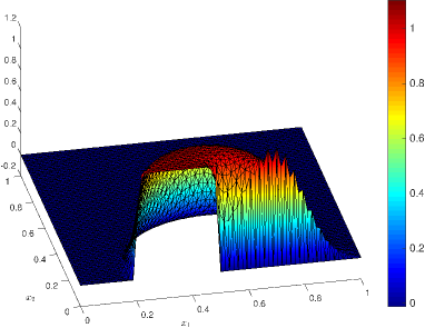
(a) Solution ${\mathcal{T}}_{8}$ (uniform, 8192 elements).

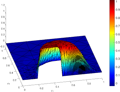
(b) Solution ${\mathcal{T}}_{14}$ (adaptive, 779 elements).

Figure 6. Convection dominated experiment from Section 4.3: The discrete FVM solution on an uniformly generated mesh ${\mathcal{T}}_{8}$ and adaptively generated mesh ${\mathcal{T}}_{14}$. The algorithm starts with a uniform initial triangulation ${\mathcal{T}}_{0}$ with $32$ elements.

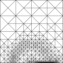
(a) ${\mathcal{T}}_{14}$ (779 elements).

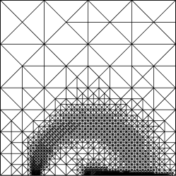
(b) ${\mathcal{T}}_{20}$ (4336 elements).

Figure 7. Convection dominated experiment from Section 4.3: Adaptively generated meshes ${\mathcal{T}}_{14}$ and ${\mathcal{T}}_{20}$ from a uniform initial triangulation ${\mathcal{T}}_{0}$ with $32$ elements.

\psfragscanon\psfrag{s05}[l][l]{\small${\rm osc}_{\ell}$ (uni.)}\psfrag{s07}[t][t]{\small number of elements}\psfrag{s01}[l][l]{\small$\eta_{\ell}$ (uni.)}\psfrag{s06}[b][b]{\small estimator, oscillation}\psfrag{s08}[l][l]{\small${\rm osc}_{\ell}$ (ada.)}\psfrag{s04}[l][l]{\scriptsize$\;\;\;1/3$}\psfrag{s12}[l][l]{\small$\eta_{\ell}$ (ada.)}\psfrag{s04}[l][l]{\scriptsize$\;\;1/2$}\psfrag{s14}[l][l]{\scriptsize$\;\;1/2$}\psfrag{s03}[l][l]{\scriptsize$1$}\psfrag{s11}[l][l]{\scriptsize$1$}\psfrag{s09}[l][l]{\scriptsize$1$}\psfrag{s13}[l][l]{\scriptsize$\;\;\;\;1$}\psfrag{x01}[t][t]{\scriptsize${10^{1}}$}\psfrag{x02}[t][t]{\scriptsize${10^{2}}$}\psfrag{x03}[t][t]{\scriptsize${10^{3}}$}\psfrag{x04}[t][t]{\scriptsize${10^{4}}$}\psfrag{x05}[t][t]{\scriptsize${10^{5}}$}\psfrag{x06}[t][t]{\scriptsize${10^{6}}$}\psfrag{v01}[r][r]{\scriptsize${10^{-6}}$}\psfrag{v02}[r][r]{\scriptsize${10^{-5}}$}\psfrag{v03}[r][r]{\scriptsize${10^{-4}}$}\psfrag{v04}[r][r]{\scriptsize${10^{-3}}$}\psfrag{v05}[r][r]{\scriptsize${10^{-2}}$}\psfrag{v06}[r][r]{\scriptsize${10^{-1}}$}\psfrag{v07}[r][r]{\scriptsize${10^{0}}$}\includegraphics[width=346.89731pt]{figures/bsp3-error.eps}

Figure 8. Convection dominated experiment from Section 4.3: Weighted-residual error estimator $\eta_{\ell}$ and data oscillations ${\rm osc}_{\ell}$ for uniform and adaptive mesh-refinement.

4.3. Convection dominated experiment

The final example is taken from [MN05]. On the square $\Omega=(0,1)^{2}$, we fix the diffusion $\mathbf{A}=10^{-3}\mathbf{I}$ and the convection velocity $\mathbf{b}=(x_{2},1/2-x_{1})^{T}$. The reaction and right-hand side are $c=f=0$. Thus, Eq. 2 holds with $\lambda_{\min}=\lambda_{\max}=10^{-3}$ and Eq. 4 with $\frac{1}{2}{\rm div}\,\mathbf{b}+c=0$. On the Dirichlet boundary $\Gamma$, we prescribe the continuous piecewise linear function by

$$u(x_{1},x_{2})|_{\Gamma}=\left\{\begin{array}[]{rl}1&\quad\text{on }\{0.2005\leq x_{1}\leq 0.4995,x_{2}=0\},\\ 0&\quad\text{on }\Gamma\backslash\{0.2\leq x_{1}\leq 0.5;x_{2}=0\}\\ \text{linear}&\quad\text{on }\{0.2\leq x_{1}\leq 0.2005\text{ or }0.4995\leq x_{1}\leq 0.5;x_{2}=0\},\end{array}\right.$$

The model has a moderate convection dominance with respect to the diffusion and simulates the transport of a pulse from $\Gamma$ to the interior and back to $\Gamma$. For this example, we do not know the analytical solution. The uniform initial mesh ${\mathcal{T}}_{0}$ consists of $32$ triangles. In Figure 66(a), we see the solution with strong oscillations on an uniformly generated mesh with $8192$ elements. The oscillations are due to the convection dominance. For the next refinement step ($16384$ elements, not plotted), however, the oscillations disappear since the shock region at the boundary is refined enough. Our adaptive Algorithm 7, which also has a mandatory oscillation marking, provides a stable solution on a mesh with only $779$ elements; see Figure 66(b). In Figure 7, we plot adaptively generated meshes after $14$ and $20$ mesh-refinements. We see a strong refinement in the shock region. A similar observation can be found in [MN05]. We remark that this strategy only works for this moderate convection dominated problem. For $\mathbf{A}=10^{-8}\mathbf{I}$, we cannot see any stabilization effects by Algorithm 7 (not displayed). Hence, only a stabilization of the numerical scheme, e.g., FVM with upwinding, would avoid these instabilities. However, the analysis of such schemes is beyond the scope of this work. We observe the above stabilization effects also in the convergence plot of the estimator; see Figure 8. Note that the estimator for adaptive mesh-refinement is faster in the asymptotic convergence than the estimator for uniform mesh-refinement. Additionally, the convergence rate for the estimator is suboptimal for uniform mesh-refinement. For adaptive mesh-refinement, we regain the optimal convergence order of ${\mathcal{O}}(N^{-1/2})$; see Figure 8. As in the previous experiments, the oscillations are of higher order. In Table 3, we also see that the oscillation marking for this convection dominated problem is for more refinement steps dominant than for the previous problems; see also the discussion in [MN05].

$\ell$	$\#{\mathcal{T}}_{\ell}$	$\frac{\#{\mathcal{M}}_{\ell}}{\#{\mathcal{M}}_{\ell}^{\eta}}$	$\frac{{\rm osc}_{\ell}({\mathcal{M}}_{\ell}^{\eta})^{2}}{{\rm osc}_{\ell}^{2}}$
0	32	1.125	0.434
1	48	1.400	0.201
2	59	1.500	0.266
3	72	1.667	0.196
4	90	2.500	0.177
5	110	1.333	0.266
6	154	1.583	0.085
7	187	1.500	0.124
8	238	1.786	0.055
9	280	1.296	0.234
10	332	1.371	0.154
11	405	1.412	0.124
12	511	1.537	0.083

$\ell$	$\#{\mathcal{T}}_{\ell}$	$\frac{\#{\mathcal{M}}_{\ell}}{\#{\mathcal{M}}_{\ell}^{\eta}}$	$\frac{{\rm osc}_{\ell}({\mathcal{M}}_{\ell}^{\eta})^{2}}{{\rm osc}_{\ell}^{2}}$
13	628	1.521	0.146
14	779	1.559	0.077
15	1,100	1.600	0.064
16	1,428	1.605	0.063
17	1,837	1.643	0.037
18	2,416	1.594	0.058
19	3,195	1.437	0.060
20	4,336	1.583	0.048
21	5,664	1.402	0.072
22	7,666	1.445	0.047
23	10,186	1.351	0.067
24	13,919	1.258	0.078
25	19,041	1.230	0.112

$\ell$	$\#{\mathcal{T}}_{\ell}$	$\frac{\#{\mathcal{M}}_{\ell}}{\#{\mathcal{M}}_{\ell}^{\eta}}$	$\frac{{\rm osc}_{\ell}({\mathcal{M}}_{\ell}^{\eta})^{2}}{{\rm osc}_{\ell}^{2}}$
26	26,248	1.182	0.106
27	36,592	1.142	0.135
28	50,806	1.112	0.180
29	70,367	1.082	0.196
30	97,946	1.058	0.227
31	135,122	1.057	0.236
32	186,959	1.028	0.311
33	255,994	1.021	0.311
34	351,880	1.022	0.289
35	484,157	1.015	0.328
36	662,325	1.006	0.381
37	902,659	1.005	0.384

Table 3. Experimental results on marking strategy for the convection dominated experiment from Section 4.3: We compute $\widetilde{C}_{MNS}:=\#{\mathcal{M}}_{\ell}/\#{\mathcal{M}}_{\ell}^{\eta}\leq 3$ and see that the additional assumption in Theorem 15 is experimentally verified. In addition, we compute $\widetilde{\theta}^{\prime}:={\rm osc}_{\ell}({\mathcal{M}}_{\ell}^{\eta})^{2}/{\rm osc}_{\ell}^{2}\geq 0.03$ with ${\rm osc}_{\ell}({\mathcal{M}}_{\ell}^{\eta})^{2}:=\sum_{T\in{\mathcal{M}}_{\ell}^{\eta}}{\rm osc}_{\ell}(T,u_{\ell})^{2}$, i.e., the choice $\theta=0.5$, $\theta^{\prime}=0.03$ would guarantee ${\mathcal{M}}_{\ell}={\mathcal{M}}_{\ell}^{\eta}$ in Algorithm 7.

5. Conclusions

In this work, we have proved linear convergence of an adaptive vertex-centered finite volume method with generically optimal algebraic rates to the solution of a general second-order linear elliptic PDE. Besides marking based on the local contributions of the a posteriori error estimator, we additionally had to mark the oscillations to overcome the lack of a classical Galerkin orthogonality property. In case of dominating convection, finite volume methods provide a natural upwind stabilization. Although there exist estimators also for these upwind discretizations [Era13], we were not able to provide a rigorous convergence result for the related adaptive mesh-refinement strategy. Note that the upwind direction and thus the corresponding error indicator contributions are defined over the boundary of the control volumes of the dual mesh. As mentioned above, the dual meshes are not nested even for a sequence of locally refined triangulations. This makes it difficult to show Eq. A1–Eq. A2 and Eq. B1–Eq. B2. We stress that the other error indicator contributions are defined over the elements of the primal mesh and can hence be treated by the developed techniques.

References

- [BDD04] P. Binev, W. Dahmen, and R. DeVore. Adaptive finite element methods with convergence rates. Numer. Math., 97(2):219–268, 2004.
- [BHP17] A. Bespalov, A. Haberl, and D. Praetorius. Adaptive fem with coarse initial mesh guarantees optimal convergence rates for compactly perturbed elliptic problems. Comput. Methods Appl. Mech. Engrg., 317:318–340, 2017.
- [BL76] J. Bergh and J. Löfström. Interpolation spaces. An introduction. Springer-Verlag, Berlin-New York, 1976. Grundlehren der Mathematischen Wissenschaften, No. 223.
- [CFPP14] C. Carstensen, M. Feischl, M. Page, and D. Praetorius. Axioms of adaptivity. Comput. Math. Appl., 67:1195–1253, 2014.
- [CKNS08] J. M. Cascón, C. Kreuzer, R. H. Nochetto, and K. G. Siebert. Quasi-optimal convergence rate for an adaptive finite element method. SIAM J. Numer. Anal., 46(5):2524–2550, 2008.
- [CLT05] C. Carstensen, R. D. Lazarov, and S. Z. Tomov. Explicit and averaging a posteriori error estimates for adaptive finite volume methods. SIAM J. Numer. Anal., 42(6):2496–2521, 2005.
- [CN12] J. M. Cascón and R. H. Nochetto. Quasioptimal cardinality of AFEM driven by nonresidual estimators. IMA J. Numer. Anal., 32(1):1–29, 2012.
- [Dör96] W. Dörfler. A convergent adaptive algorithm for Poisson’s equation. SIAM J. Numer. Anal., 33(3):1106–1124, 1996.
- [ELL02] R. E. Ewing, T. Lin, and Y. Lin. On the accuracy of the finite volume element method based on piecewise linear polynomials. SIAM J. Numer. Anal., 39(6):1865–1888, 2002.
- [EP16] C. Erath and D. Praetorius. Adaptive vertex-centered finite volume methods with convergence rates. SIAM J. Numer. Anal., 54(4):2228–2255, 2016.
- [EP17] C. Erath and D. Praetorius. Céa-type quasi-optimality and convergence rates for (adaptive) vertex-centered FVM. In C. Cancès and P. Omnes, editors, Finite Volumes for Complex Applications VIII - Methods and Theoretical Aspects, volume 199, pages 215–223. Springer, Berlin, 2017.
- [Era10] C. Erath. Coupling of the Finite Volume Method and the Boundary Element Method - Theory, Analysis, and Numerics. PhD thesis, University of Ulm, 2010.
- [Era12] C. Erath. Coupling of the finite volume element method and the boundary element method: an a priori convergence result. SIAM J. Numer. Anal., 50(2):574–594, 2012.
- [Era13] C. Erath. A posteriori error estimates and adaptive mesh refinement for the coupling of the finite volume method and the boundary element method. SIAM J. Numer. Anal., 51(3):1777–1804, 2013.
- [FFP14] M. Feischl, T. Führer, and D. Praetorius. Adaptive FEM with optimal convergence rates for a certain class of nonsymmetric and possibly nonlinear problems. SIAM J. Numer. Anal., 52(2):601–625, 2014.
- [Gri85] P. Grisvard. Elliptic Problems in Nonsmooth Domains. Pitman, Boston, 1985.
- [KPP13] M. Karkulik, D. Pavlicek, and D. Praetorius. On 2D newest vertex bisection: optimality of mesh-closure and -stability of -projection. Constr. Approx., 38(2):213–234, 2013.
- [MN05] K. Mekchay and R. H. Nochetto. Convergence of adaptive finite element methods for general second order linear elliptic PDEs. SIAM J. Numer. Anal., 43(5):1803–1827, 2005.
- [MNS00] P. Morin, R. H. Nochetto, and K. G. Siebert. Data oscillation and convergence of adaptive FEM. SIAM J. Numer. Anal., 38(2):466–488, 2000.
- [Ste07] R. Stevenson. Optimality of a standard adaptive finite element method. Found. Comput. Math., 7(2):245–269, 2007.
- [Ste08] R. Stevenson. The completion of locally refined simplicial partitions created by bisection. Math. Comp., 77(261):227–241, 2008.
- [SZ90] L. R. Scott and S. Zhang. Finite element interpolation of nonsmooth functions satisfying boundary conditions. Math. Comp., 54(190):483–493, 1990.