Hidden edge Dirac point and robust quantum edge transport in InAs/GaSb quantum wells

Abstract

The robustness of quantum edge transport in InAs/GaSb quantum wells in the presence of magnetic fields raises an issue on the fate of topological phases of matter under time-reversal symmetry breaking. A peculiar band structure evolution in InAs/GaSb quantum wells is revealed: the electron subbands cross the heavy hole subbands but anticross the light hole subbands. The topologically protected band crossing point (Dirac point) of the helical edge states is pulled to be close to and even buried in the bulk valence bands when the system is in a deeply inverted regime, which is attributed to the existence of the light hole subbands. A sizable Zeeman energy gap verified by the effective g-factors of edge states opens at the Dirac point by an in-plane or perpendicular magnetic field, however it can also be hidden in the bulk valance bands. This provides a plausible explanation for the recent observation on the robustness of quantum edge transport in InAs/GaSb quantum wells subjected to strong magnetic fields.

I Introduction

The quantum spin Hall (QSH) insulator is a quantum state of matter with topologically protected helical edge states in the bulk insulating gap Hasan and Kane (2010); Qi and Zhang (2011); Shen (2017). The helical edge states will give rise to the QSH effect which is featured by a quantized conductance (i.e., $2e^{2}/h$) in the two-terminal measurement at low temperatures Kane and Mele (2005). Theoretically the band crossing point (Dirac point) of the helical edge states is topologically protected by time-reversal symmetry, and it opens a minigap once the symmetry is broken (if there is no other extra symmetry protection). The QSH insulator has been predicted theoretically Bernevig et al. (2006) and confirmed experimentally in HgTe/CdTe quantum wells König et al. (2007); Roth et al. (2009). Another promising candidate for QSH insulator is the InAs/GaSb double quantum well Liu et al. (2008); Knez et al. (2011). The InAs/GaSb quantum wells possess a particular electronic phase with inverted band structure, in which the hybridization of electrons and holes opens a minigap at finite $k$-vectors, leading to the QSH phase. Due to the mature technology of material fabrications and potential device applications, there have been growing efforts exploring the QSH phase in InAs/GaSb quantum wells Knez et al. (2010, 2011); Suzuki et al. (2013); Nichele et al. (2014); Mueller et al. (2015); Qu et al. (2015); Nguyen et al. (2016); Karalic et al. (2016); Nichele et al. (2017). Recently, it was observed that the conductance in InAs/GaSb quantum wells can keep quantized in an in-plane magnetic field up to 12 T and is insensitive to temperatures ranging from 250 mK to several Kelvins Du et al. (2015). Similar feature was also observed in HgTe/CdTe quantum wells Ma et al. (2015). This raises a question about the fate of the QSH effect under time-reversal symmetry breaking, which has become a fundamental issue to understand the physics of topological matter. A number of theoretical efforts have been simulated on this puzzle Pikulin et al. (2014); Zhang et al. (2014); Hu et al. (2016). However the robustness of the quantized conductance remains poorly understood.

In InAs/GaSb quantum wells, the lowest conduction bands of InAs are about 150 meV lower than the highest valence bands of GaSb Altarelli (1983); Yang et al. (1997), which forms a broken-gap band alignment and leads to the coexistence of electrons and holes near the charge neutrality point. The application of gate voltages can shift the band alignment and drive the system to different electronic phases Naveh and Laikhtman (1995); Liu et al. (2008); Qu et al. (2015). When the (lowest) electron subbands of InAs lie above the (highest) heavy hole (HH) subbands of GaSb, the system is in a normal insulator phase. Whereas the electron subbands lie below the HH subbands, the system is in an inverted phase and the QSH effect is expected in the hybridization gap opened by coupling between electron and hole states. Around the topological phase transition point, the system can be well described by Bernevig-Hughes-Zhang (BHZ) model which considers four bands in the lowest energy Bernevig et al. (2006); Liu et al. (2008). The BHZ model, however, fails to explain the robust quantum edge transport in InAs/GaSb quantum wells in the presence of in-plane magnetic fields, in which the Dirac point of the helical edge states opens an mini-gap, leading to the breakdown of quantized conductance. InAs/GaSb quantum wells could possibly be in a deeply inverted regime where the lower energy subbands, e.g., the light hole (LH) subbands, will reside above the electron subbands and may have important influence on the system. The consideration of the LH subbands may be a resolution to the puzzle. To this end, re-examination of the band structure of InAs/GaSb quantum wells and a more comprehensive effective model are needed.

In the present work, a peculiar band structure evolution in InAs/GaSb quantum wells is revealed when varying the gate voltages. The electron subbands of InAs can cross the HH subbands of GaSb, and correspondingly the system transits between a trivial insulator phase and a topological insulator phase as described by the BHZ model. In contrast, the electron subbands cannot touch but anticross the LH subbands of GaSb. This anticrossing behavior does not alter the topology of the system as no gap closing occurs, however, it may modify the properties of system near the hybridization gap significantly. We present a six-band effective model to capture the essential low-energy properties of InAs/GaSb quantum wells, including the topological phase transition and anticrossing behavior. One of the key features is that the Dirac point of the edge states will be pulled to be close to the bulk valence bands when the electron subbands are lowered to anticross the LH subbands. The application of a magnetic field, in-plane or perpendicular, opens a sizable Zeeman energy gap at the Dirac point of the helical edge states, which indicates the breaking down of the QSH effect. Nevertheless, the energy gap of edge states could also be hidden in the bulk valence bands up to a large magnetic field, which may account for recent experimental observation on the robustness of quantum edge transport under in-plane magnetic fields Du et al. (2015). We anticipate our results can shed some light on experimental observations on the InAs/GaSb quantum wells and explore novel topological phases of matter in the future.

The rest of this paper is organized as follows. In Sec. II the band structure evolution of InAs/GaSb quantum wells is studied, and in Sec. III a six-band effective model is derived for low-energy physics of the quantum wells. With the effective model, the properties of edge states are investigated in Sec. IV. To characterize the response of the helical edge states to magnetic fields, the effective g-factors of edge states are calculated in Sec. V. In Sec. VI the robustness of quantum edge transport under in-plane magnetic fields is addressed by the numerical calculation of conductance. Finally, Sec. VII contains the discussions and conclusions.

II Band structure evolution of $\mathrm{InAs/GaSb}$ quantum wells

Both InAs and GaSb have zinc-blende crystal structure and direct gaps near the $\Gamma$ point, and their low-energy physics can be well described by the Kane model Kane (1957); Winkler (2003). Considering the broken-gap band alignment in InAs/GaSb quantum wells and focusing on the case where the $\Gamma^{6}$ bands of InAs and the $\Gamma^{8}$ bands of GaSb are very close while the $\Gamma^{7}$ bands are far away in energy and thus can be neglected here. In the basis $\{|\Gamma^{6},1/2\rangle,|\Gamma^{6},-1/2\rangle,|\Gamma^{8},3/2\rangle,|\Gamma^{8},1/2\rangle,|\Gamma^{8},-1/2\rangle,$ $|\Gamma^{8},-3/2\rangle\}$ (Here we use the standard notation that $|\Gamma^{6},\pm 1/2\rangle,$ $|\Gamma^{8},\pm 1/2\rangle$ and $|\Gamma^{8},\pm 3/2\rangle$ represent the s-like conduction bands, the p-like LH bands, and the p-like HH bands, respectively), the Kane Hamiltonian for the [001] growth direction is given by Winkler (2003); Novik et al. (2005)

$$H=\left(\begin{array}[]{cccccc}T&0&-\frac{1}{\sqrt{2}}Pk_{+}&\sqrt{\frac{2}{3}}Pk_{z}&\frac{1}{\sqrt{6}}Pk_{-}&0\\ 0&T&0&-\frac{1}{\sqrt{6}}Pk_{+}&\sqrt{\frac{2}{3}}Pk_{z}&\frac{1}{\sqrt{2}}Pk_{-}\\ -\frac{1}{\sqrt{2}}k_{-}P&0&U+V&-\bar{S}_{-}&R&0\\ \sqrt{\frac{2}{3}}k_{z}P&-\frac{1}{\sqrt{6}}k_{-}P&-\bar{S}_{-}^{\dagger}&U-V&C&R\\ \frac{1}{\sqrt{6}}k_{+}P&\sqrt{\frac{2}{3}}k_{z}P&R^{\dagger}&C^{\dagger}&U-V&\bar{S}_{+}^{\dagger}\\ 0&\frac{1}{\sqrt{2}}k_{+}P&0&R^{\dagger}&\bar{S}_{+}&U+V\end{array}\right),$$ (1)

where

$$T =E_{c}+h^{\prime}(\gamma_{0}k_{||}^{2}+k_{z}\gamma_{0}k_{z}),$$

$$U =E_{v}-h^{\prime}(\gamma_{1}k_{||}^{2}+k_{z}\gamma_{1}k_{z}),$$

$$V =-h^{\prime}(\gamma_{2}k_{||}^{2}-2k_{z}\gamma_{2}k_{z}),$$

$$R =\sqrt{3}h^{\prime}\gamma_{2}(k_{x}^{2}-k_{y}^{2})-2\sqrt{3}ih^{\prime}\gamma_{3}k_{x}k_{y},$$

$$\bar{S}_{\pm} =-\sqrt{3}h^{\prime}k_{\pm}\left(\{\gamma_{3},k_{z}\}+[\kappa,k_{z}]\right),$$

$$C =2h^{\prime}k_{-}[\kappa,k_{z}],$$ (2)

in which ${\bf k}_{\parallel}=(k_{x},k_{y})$, $k_{||}^{2}=k_{x}^{2}+k_{y}^{2}$, $k_{\pm}=k_{x}\pm ik_{y}$, and $h^{\prime}=\hbar^{2}/(2m_{0})$. $m_{0}$ is the free electron mass, and $P$ is the Kane momentum matrix element. $E_{c}$ and $E_{v}$ are the conduction and valence band edges, respectively. $\gamma_{0,1,2,3}$ and $\kappa$ are the band parameters in the Kane model. The parameters for InAs, GaSb and AlSb are given in Table 1. We consider the quantum well configuration with InAs and GaSb layers sandwiched by two AlSb layers at each side along the growth direction (the $z$-direction). Hence the parameters of the Kane model are spatial dependent, corresponding to different layers of the quantum wells. To simulate the experimental setup and for illustration, we will take 12.5 nm InAs/10 nm GaSb with barriers made of 50 nm AlSb at each side in the quantum well system Du et al. (2015).

Table 1: Parameters in the Kane model for InAs, GaSb and AlSb Lawaetz (1971); Halvorsen et al. (2000); Nichele et al. (2017).

	$E_{g}$[eV]	$P$[eV$\cdot\mathrm{\textrm{\r{A}}}$]	$\gamma_{1}$	$\gamma_{2}$	$\gamma_{3}$	$\gamma_{0}$	$\kappa$	$E_{c}$[eV]	$E_{v}$[eV)]
InAs	0.41	9.19	19.67	8.37	9.29	1/0.03	7.68	-0.15	-0.56
GaSb	0.8128	9.23	11.8	4.03	5.26	1/0.042	3.18	0.8128	0
AlSb	2.32	8.43	4.15	1.01	1.75	1/0.18	0.31	1.94	-0.38

Table 2: Parameters in the six-band effective model for $V_{0}$=-100meV, $L_{\text{InAs}}=12.5$ nm, $L_{\text{GaSb}}=10$ nm and $L_{\text{AlSb}}=50$ nm.

Parameters	$B_{e}$[eV$\cdot\mathrm{\mathring{A}}^{2}$]	$B_{h}$[eV$\cdot\mathrm{\mathring{A}}^{2}$]	$B_{l}$[eV$\cdot\mathrm{\mathring{A}}^{2}$]	$D_{el}$[eV$\cdot\mathrm{\mathring{A}}^{2}$]	$P_{eh}$[eV$\mathrm{\cdot\textrm{\r{A}}}$]	$P_{el}$[eV$\cdot\mathrm{\textrm{\r{A}}}$]	$P_{lh}$[eV$\mathrm{\cdot\textrm{\r{A}}}$]	$P_{e}$[eV$\cdot\mathrm{\textrm{\r{A}}}$]	$P_{l}$[eV$\mathrm{\cdot\textrm{\r{A}}}$]
Value	81.3	-31.2	-60	40	0.45	0.11	0.61	0.13	0.29
Parameters	$\gamma_{2eh}$	$\gamma_{3eh}$	$\gamma_{2lh}$	$\gamma_{3lh}$	$Q_{e}$[eV]	$Q_{l}$[eV]	$Q_{el}$[eV]	$E_{e}$[eV]	$E_{h}$[eV]	$E_{l}$[eV]
Value	1.88	2.45	-3.3	-4.3	0.76	0.21	0.38	-0.0283	-0.0115	–0.0529

We assume the confinement effect in the $z$-direction and replace the operator $k_{z}$ with $-i\partial_{z}$ in the Hamiltonian. The full Hamiltonian of the quantum wells takes the form

$$H_{\text{full}}=H_{K}(k_{x},k_{y},-i\partial_{z})+V(z).$$ (3)

Here $V(z)$ is the confinement potential and is also spatial dependent. The subbands dispersions and corresponding eigenstates are obtained by solving the Schrödinger equation:

$$H_{\text{full}}|\Psi^{\xi}(k_{x},k_{y},z)\rangle=E^{\xi}|\Psi^{\xi}(k_{x},k_{y},z)\rangle,$$ (4)

where $\xi$ is the subband index, and $|\Psi^{\xi}(k_{x},k_{y},z)\rangle=\exp[ik_{x}x+ik_{y}y]F^{\xi}(z)$ with $F^{\xi}(z)$ an envelope function. The envelope function approximation can be employed to solve the eigen problem of the quantum wells Li et al. (2009). $F^{\xi}(z)$ can be expanded in terms of plane waves

$$F^{\xi}(z)=\sum_{\lambda=1}^{6}\sum_{n=-N}^{N}\frac{1}{\sqrt{L}}a_{n,\lambda}^{\xi}e^{ik_{n}z}|\lambda\rangle,$$ (5)

where $k_{n}=2\pi n/L$ with $n=0,\pm 1,\pm 2,\cdots,\pm N$ ($N$ is a positive integer), and $L=L_{\mathrm{InAs}}+L_{\mathrm{GaSb}}+2L_{\mathrm{AlSb}}$ is the total width of InAs/GaSb quantum wells. $a_{n,\lambda}^{\xi}$ are the corresponding expansion coefficients. Here we use $|\lambda\rangle$ ($\lambda$ = 1, 2, $\cdots$ , 6) to denote the basis set of wave functions where $|1\rangle$ and $|2\rangle$ are for $|\Gamma^{6},\pm 1/2\rangle$, $|3\rangle$ and $|6\rangle$ are for $|\Gamma^{8},\pm 3/2\rangle$, and $|4\rangle$ and $|5\rangle$ are for $|\Gamma^{8},\pm 1/2\rangle$. For the numerical calculations, we take $N=30$ which is accurate enough for the low-energy physics.

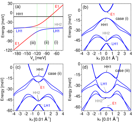
Figure 1: The energy spectrum of InAs/GaSb quantum wells in different phases. (a) The energies of the lowest-energy subbands at the $\Gamma$ point as functions of the broken gap $V_{0}$. The band structures at $k_{y}=0$ with (b) $V_{0}=-70$ meV; (c) $V_{0}=-90$ meV; (d) $V_{0}=-120$ meV.

Different electronic phases can be realized by varying the broken gap $V_{0}$, the energy difference of band edges between the $\Gamma^{6}$ bands of InAs and the $\Gamma^{8}$ bands of GaSb, which is supposed to be tunable by gate voltages Liu et al. (2008); Qu et al. (2015). Figure 1(a) shows the energies of the lowest energy subbands at the $\Gamma$ point as functions of $V_{0}$. One can see that when decreasing $V_{0}$, the lowest electron ($E1$) subbands cross the highest HH ($HH1$) subbands, showing a topological phase transition. For a large $V_{0}(>-80$ meV), the system is a trivial insulator as shown in Fig. 1(b) and should not possess robust edge states, which is labeled as case (i). For a smaller $V_{0}(<-80$ meV), the system transfers from the trivial insulating phase to a shallowly inverted phase labeled by case (ii). A hybridization gap will open at the crossing point, as shown in Fig. 1(c), and the QSH effect is expected Liu et al. (2008). The low-energy properties of the system near the phase transition point $V_{0}(\sim-80$ meV) can be well described by the BHZ model Bernevig et al. (2006). Decreasing $V_{0}$ further, the $E1$ subbands does not touch but anticross the highest LH ($LH1$) subbands. We label the deeply inverted phase after the anticrossing as case (iii). The transition from cases (ii) to (iii) is topologically trivial since there is no gap closing, however, some important properties (e.g., the property of edge states) near the system gap are changed, as will be shown below. The corresponding band structure for case (iii) is presented in Fig. 1(d), which exhibits giant spin-orbit splitting close to the hybridization gap. The spin-orbit splitting due to the structure inversion asymmetry may lead to fully spin polarized states Nichele et al. (2017).

III Six-band effective model

The topologically non-trivial band structure indicates the existence of helical edge states across bulk insulating gap with the open boundaries according to the bulk-edge correspondence Hatsugai (1993); Qi et al. (2006); Graf and Porta (2013). To find the helical edge states and investigate the low-energy properties of InAs/GaSb quantum wells, it is helpful to derive an effective model, just as the BHZ model Bernevig et al. (2006). Noting that without gate voltage the InAs/GaSb quantum wells tend to stay in the deeply inverted phase of case (iii), the $LH1$ subbands may have significant influence on the system and thus should also be considered. A six-band effective model which involves the $E1$, $HH1$ and $LH1$ subbands can be constructed, following a similar procedure of Refs. Bernevig et al. (2006); Rothe et al. (2010).

Generally the full bulk Hamiltonian can be split into two parts

$$H_{\text{full}}=H_{0}({\bf k}_{\parallel}=0,-i\partial_{z},z)+H^{\prime}({\bf k}_{\parallel},-i\partial_{z},z),$$ (6)

where $H_{0}$ describes the system at the $\Gamma$ point (i.e., ${\bf k}_{\parallel}=0)$ and $H^{\prime}$ can be treated as a perturbation around the $\Gamma$ point. First, we can numerically solve the Schrödinger equation $H_{0}|\Psi_{0}^{\xi}\rangle=E_{0}^{\xi}|\Psi_{0}^{\xi}\rangle$ and obtain the eigenenergies $E_{0}^{\xi}$ and the corresponding eigenstates $|\Psi_{0}^{\xi}\rangle$. The Hamiltonian $H_{0}$ is effectively decoupled to four blocks: the electron subbands couple only with the LH subbands, while the HH subbands decouple from them. We can treat these decoupled blocks separately. Three eigen wave functions with components of the $E1$ and $HH1$ bands, or of the $LH1$ subbands can be written as

$$\langle z|E1,+\rangle =\left(\psi_{e1}(z),0,0,\psi_{e4}(z),0,0\right)^{T},$$ (7)

$$\langle z|HH1,+\rangle =\left(0,0,\psi_{h3}(z),0,0,0\right)^{T},$$ (8)

$$\langle z|LH1,+\rangle =\left(\psi_{l1}(z),0,0,\psi_{l4}(z),0,0\right)^{T},$$ (9)

where $T$ means transpose. The envelope function components $\psi_{e(h,l)}(z)$ can be found by expanding the eigenstates in terms of plane waves, as introduced previously. Carrying out the time-reversal operation on the above wave functions, we have other three eigen wave functions

$$\langle z|E1,-\rangle =\left(0,\psi_{e1}^{*}(z),0,0,-\psi_{e4}^{*}(z),0\right)^{T},$$ (10)

$$\langle z|HH1,-\rangle =\left(0,0,0,0,0,\psi_{h3}^{*}(z)\right)^{T},$$ (11)

$$\langle z|LH1,-\rangle =\left(0,-\psi_{l1}^{*}(z),0,0,\psi_{l4}^{*}(z),0\right)^{T}.$$ (12)

Next, with the six lowest energy states at the $\Gamma$ point as a basis set, we can project the Hamiltonian (6) and obtain a two-dimensional six-band effective model. In the ordered basis $\left\{|E1,+\rangle,|E1,-\rangle,\right.$$|HH1,+\rangle,$ $|LH1,+\rangle,\left.|LH1,-\rangle,|HH1,-\rangle\right\}$, the effective Hamiltonian reads

$$H ({\bf k}_{\parallel})=H_{0}({\bf k}_{\parallel})+\delta H,$$ (13)

$$H_{0}({\bf k}_{\parallel}) =\left(\begin{array}[]{cccccc}T_{e}&-\frac{P_{e}k_{-}}{\sqrt{6}}&-\frac{P_{eh}k_{+}}{\sqrt{2}}&Dk^{2}&\frac{P_{el}k_{-}}{\sqrt{6}}&R_{eh}\\ -\frac{P_{e}k_{+}}{\sqrt{6}}&T_{e}&-R_{eh}^{\dagger}&-\frac{P_{el}k_{+}}{\sqrt{6}}&-Dk^{2}&\frac{P_{eh}k_{-}}{\sqrt{2}}\\ -\frac{P_{eh}k_{-}}{\sqrt{2}}&-R_{eh}&T_{h}&-\frac{P_{lh}k_{-}}{\sqrt{2}}&R_{lh}&0\\ Dk^{2}&-\frac{P_{el}k_{-}}{\sqrt{6}}&-\frac{P_{lh}k_{+}}{\sqrt{2}}&T_{l}&\frac{P_{l}k_{-}}{\sqrt{6}}&R_{lh}\\ \frac{P_{el}k_{+}}{\sqrt{6}}&-Dk^{2}&R_{lh}^{\dagger}&\frac{P_{l}k_{+}}{\sqrt{6}}&T_{l}&-\frac{P_{lh}k_{-}}{\sqrt{2}}\\ R_{eh}^{\dagger}&\frac{P_{eh}k_{+}}{\sqrt{2}}&0&R_{lh}^{\dagger}&-\frac{P_{lh}k_{+}}{\sqrt{2}}&T_{h}\end{array}\right),$$ (20)

$$\delta H =\Delta V\left(\begin{array}[]{cccccc}Q_{e}&0&0&Q_{el}&0&0\\ 0&Q_{e}&0&0&-Q_{el}&0\\ 0&0&0&0&0&0\\ Q_{el}&0&0&Q_{l}&0&0\\ 0&-Q_{el}&0&0&Q_{l}&0\\ 0&0&0&0&0&0\end{array}\right)$$ (27)

where $k_{\pm}=k_{x}\pm ik_{y}$, $T_{e(l,h)}=E_{e(l,h)}+B_{e(l,h)}k_{\parallel}^{2}$, and $R_{e(l)h}=\sqrt{3}h^{\prime}\gamma_{2e(l)h}(k_{x}^{2}-k_{y}^{2})-i2\sqrt{3}h^{\prime}\gamma{}_{3e(l)h}k_{x}k_{y}$. Here and after, we choose a fixed broken gap $V_{0}$ as reference and take $\Delta V$ as a variation from $V_{0}$ to tune the band structure evolution for convenience. $H_{0}({\bf k}_{\parallel})$ describes the system with the broken gap $V_{0}$. $\delta H$ is the modification by $\Delta V$, the small change of the broken gap, it shows clearly how the whole band structure varies as tuning gate voltages. The diagonal terms $Q_{e}$ and $Q_{l}$ in $\Delta H$ will shift the position of $E1$ and $LH1$ subbands, as shown in Fig. 1(a). There is no diagonal term for the $HH1$ subbands in $\Delta H$, which is consistent with Fig. 1(a) in which the $HH1$ subbands nearly do not shift. The off-diagonal term $Q_{el}$ is crucial for the anticrossing behavior. It couples the $E1$ and $LH1$ subbands even at the $\Gamma(k_{x}=k_{y}=0)$ point, preventing them from touching with each other. In this way, the effective model not only covers the physics of the BHZ model but also captures the anticrossing behavior of the energy bands. The parameters in this effective Hamiltonian can be found straightforwardly in the projection, and they depend on the details of the quantum wells (i.e., the thickness of the quantum wells and the broken gap reference $V_{0}$, etc.). For the considered quantum well configuration (i.e., the thickness of 50/12.5/10/50 nm for AlSb/InAs/GaSb/AlSb), the parameters in the effect model are provided in Table 2.

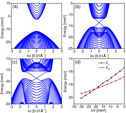
Figure 2: Energy spectrum of bulk and edge states of the system with periodic and open boundaries in the $x$ and $y$ direction, respectively. (a) for $\Delta V=30$ meV , (b) for $\Delta V=10$ meV, (c) for $\Delta V=-20$ meV, and (d) the energy position of Dirac point ($E_{D}$) and maximum point of valence bands ($E_{M}$) as function of $\Delta V$. $V_{0}=-100$ meV is taken for all figures.

IV Hidden Dirac point of the helical edge states

With the six-band effective model, we are in a position to investigate the energy dispersions of the edge states for the topologically non-trivial cases (ii) and (iii). This can be accomplished numerically by means of tight-binding calculations. The tight-binding model can be obtained by discretizing the effective Hamiltonian Eq. (13) on a square lattice. In the long wavelength limit, we use the approximation $k_{i}\approx\sin(k_{i}a)/a$ and $k_{i}^{2}\approx 2[1-\cos(k_{i}a)]/a^{2}$ with $i=x,\ y$ and $a$ the lattice constant. We take $a=20\mathring{\mathrm{A}}$ which is a good approximation to the continuum limit. To find the edge states solution, we apply the open boundary condition along the $y$ direction while the periodic boundary condition along the $x$ direction. Thus $k_{x}$ remains a good quantum number and the system is diagonal in $k_{x}$.

Figures 2(a)-(c) plot the energy spectrum of the effective model in the absence of external fields, corresponding to the cases (i)-(iii) as mentioned above. For the trivial insulator case (i), there is a direct system gap and no edge dispersion as shown in Fig. 2(a). In both cases (ii) and (iii) as shown in Figs. 2(b) and (c), there are two pairs of gapless and doubly degenerate helical edge bands across the bulk insulating gap, as expected for the QSH effect. Nevertheless, for case (iii) the Dirac point of the helical edge states is close to and even “buried” by the bulk valence states, which is in contrast to case (ii) where the Dirac point is well exposed in the middle of the bulk gap [see Fig. 2(b)]. As reducing $\Delta V$ further, the Dirac point $E_{D}$ approaches the maximum point of the bulk valence bands $E_{M}$, and eventually it is hidden by the bulk valence bands, as shown in Fig. 2(d).

The hidden Dirac point of edge states in case (iii) can be attributed to the anticrossing between $E1$ and $LH1$ subbands by comparing with Fig. 1(a). We find that the Dirac point can be hidden only around the value of $\Delta V$ where the anticrossing behavior occurs. The Dirac point will not be buried in the bulk states but well exposed in the bulk gap if the $LH1$ subbands are not taken into account. The hidden Dirac point is also related to the strong anisotropy in the system, which inherits from the bulk Kane model. The finding that the Dirac point of edge states can be hidden in the bulk bands serves as the basis for the robust quantum edge transport in InAs/GaSb quantum wells under time-reversal breaking as will be discussed in the following, and it is one of our main results.

V Effective $g$-factors of edge states

A magnetic field ${\bf B}$ breaks time-reversal symmetry, and consequently the Dirac point of the edge states will no longer be topologically protected if there is no other hidden symmetry. The time-reversal symmetry breaking can be evidenced by a gap opening in the helical edge states, which originates from the Zeeman and the orbital coupling effects of the bulk electrons in an external magnetic field. In the six-band effective model, the Zeeman term can be written as

$$H_{Z}=H_{c}^{Z}\varoplus H_{v}^{Z},$$ (28)

with

$$H_{c}^{Z}=(1/2)g_{e}\mu_{B}{\bf s}\cdot{\bf B},$$ (29)

for electrons in the s-like $E1$ bands, and

$$H_{v}^{Z}=g_{h}\mu_{B}{\bf J}\cdot{\bf B}.$$ (30)

for the p-like $HH1$ and $LH1$ bands Winkler (2003); Beugeling et al. (2012). Here ${\bf s}=\left\{s_{x},s_{y},s_{z}\right\}$ are the Pauli matrices for spin 1/2, ${\bf J}$ are the $4\times 4$ angular momentum matrices for $j=3/2$, and $\mu_{B}$ is the Bohr magneton. $g_{e}$ and $g_{h}$ are the g-factors for bulk electrons and holes, respectively, and are taken to be $g_{e}$$=-10.0$ and $g_{h}$$=0.3$ Zakharova et al. (2003); Mu et al. (2016) in the following.

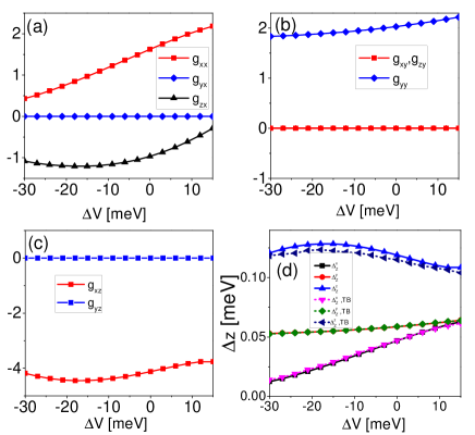
Figure 3: Effective g-factors of edge states and Zeeman energy gaps for edge states spectrum. The effective g-factor tensor elements of the edge states as function of $\Delta V$ for magnetic field along (a) $x$, (b) $y$, and (c) $z$ direction, respectively. (d) The energy gaps $\Delta_{Z}^{x,y,z}$ of edge states opened by three principal magnetic field of 0.5 T as functions of $\Delta V$. $V_{0}=-100$ meV is taken for all figures.

The response of the helical edge states to the magnetic fields can be examined by projecting the Zeeman term in the space spanned by the two helical edge states $|\psi_{0+}\rangle$ and $|\psi_{0-}\rangle$ at the $\Gamma$ point. Note that $|\psi_{0+}\rangle$ and $|\psi_{0-}\rangle$ are time-reversal to each other. The corresponding effective Zeeman coupling can be summarized as

$$\mathcal{H}_{\text{edge}}^{Z}=\dfrac{\mu_{B}}{2}\sum_{i,j=x,y,z}g_{ij}\sigma_{i}B_{j},$$ (31)

where the $g_{ij}$ is the effective g-factor tensor and $\sigma_{x,y,z}$ are the Pauli matrices for the edge states space. Reminding that the effective model for the helical edge states takes the form $\mathcal{H}_{\text{edge}}^{0}=\hbar v_{F}k_{x}\sigma_{z}$ where $v_{F}$ is the effective velocity.

The g-factor tensor is attributed to the the fact that the two helical edge states at the $\Gamma$ point are not the eigenstates of electron spin. Figures 3(a,b,c) plot the values of the g-factor elements $g_{ij}$ for different $\Delta V$, from which several points are worthy addressing. For a perpendicular magnetic field $B_{z}$, considering the contribution from the orbital angular momentum coupling to $B_{z}$, a large value of $g_{zz}$ is obtained. This large $g_{zz}$ just shifts the position of the degeneracy (Dirac) point of the helical edge states in the $k_{x}$ direction, whereas it does not open an energy gap (so we do not show it here). However, a non-zero $g_{xz}$ does open an energy gap. Here the Peierls substitution is performed as $t^{ij}\rightarrow t^{ij}\exp[\frac{2\pi i}{\phi_{0}}\int_{i}^{j}d{\bf\boldsymbol{\ell}}\cdot{\bf A}]$ where $\phi_{0}=h/e$ is the magnetic flux quantum, and $t^{ij}$ is the hopping integral between sites $i$ and $j$. For an in-plane field, the orbital contribution to g-factors is ignorable as electrons are confined in the quantum wells. $g_{xx}$ and $g_{yy}$ always take non-zero values, which indicates that an in-plane magnetic field also opens a gap in the edge states. These values of Zeeman gap calculated from the effective g-factor tensor of edge states match well with those obtained directly from the spectrum [see Fig. 3(d)]. Therefore the non-zero g-factors indicate an opened gap at the Dirac point of helical edge states under time-reversal symmetry breaking Yang et al. (2011), and the QSH effect is broken down. It is also interesting to find that the effective g-factors of edge states show an evident anisotropy. Especially for the in-plane magnetic fields, though both edge Zeeman gaps $\Delta_{\text{Z }}^{x,y}$ decay as decreasing $\Delta V$, $\Delta_{\text{Z }}^{x}$ decays much faster, which indicates that the anisotropy is enhanced for a small $\Delta V$. Finally, we note that $\Delta_{\text{Z }}^{x,y}$ can reach the order of 1 meV for a magnetic field of 10 T, which are experimentally measurable at low temperatures. However, these Zeeman gap $\Delta_{Z}^{x,y}$ could be hidden since the Dirac point would be hidden by the bulk valence bands after the anticrossing behavior at a small $\Delta V$.

VI Robustness of the quantum edge transport

Now let us address the robustness of the edge transport in the InAs/GaSb quantum wells in the inverted regime. It is known that the quantized two-terminal conductance $2e^{2}/h$ of a QSH insulator is a consequence of the helical edge states, which has been measured experimentally in the InAs/GaSb quantum wells. Unexpectedly under in-plane magnetic fields either along or normal to the boundary the quantized conductance value remains quantized for mesoscopic samples and persists up to 12 T Du et al. (2015). To understand the robustness of quantized conductance plateau, the evolution of the band structure subjected to an in-plane external magnetic field has been explored. The in-plane magnetic field effect can be included by considering that the InAs and GaSb layers are spatially separated Yang et al. (1997); Qu et al. (2015); Hu et al. (2016). An in-plane magnetic field applied along the open boundary $B_{y}$ will not only open an energy gap at the Dirac point of the edge states, but also tilt the bulk energy spectra and reduce the bulk gap Qu et al. (2015); Hu et al. (2016). Henceforth, there is no direct gap between the edge states and the valence bands if the Dirac point is buried in the bulk. Similar effect happens for the in-plane magnetic field $B_{x}$ normal to the open boundary.

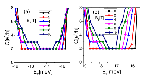
Figure 4: The two-terminal conductance $G$ of InAs/GaSb quantum wells in magnetic fields. (a) $G$ as a function of the Fermi energy $E_{F}$ in the presence of different magnetic field $B_{x}$ along the $x$ direction. (b) the same as (a) but with the magnetic fields applied along the $y$ direction. $\Delta V=-20$ meV and $V_{0}=-100$ meV are taken for both figures.

Consider a ribbon geometry of the InAs/GaSb quantum wells. The two-terminal conductance is calculated as a function of the Fermi energy $E_{F}$ under different in-plane magnetic fields by means of the Landauer-Büttiker formalism in a clean sample. The sample geometry considered consists of a rectangular central region (size $L_{x}\times L_{y}=200a\times 150a$) and two semi-infinite leads are connected to it as source and drain leads. With the help of recursive Green’s function technique Sancho et al. (1985); MacKinnon (1985), the conductance from the left terminal to the right terminal can be evaluated as

$$G=\frac{e^{2}}{h}\mathrm{Tr}\left[\Gamma_{L}G^{r}\Gamma_{R}G^{a}\right],$$ (32)

where $\Gamma_{L,R}$ are the line-width functions coupling to the left lead and the right lead respectively, and $G^{r}(G^{a})$ is the retarded (advanced) Green’s function of the central region Datta (1995).

In the absence of a magnetic field, the value of two-terminal conductance is exactly quantized at $G=2e^{2}/h$ as predicted theoretically for the QSH effect. The conductance remains nearly unchanged for different magnetic fields either along the boundary as shown in Fig. 4(a) or normal to the boundary as shown in Fig. 4(b), which can be attributed to the fact that the energy gap of edge states is buried in the bulk valence bands. This support that the picture of hidden Dirac point may account for the experimental observations on robust quantum edge transport in InAs/GaSb quantum wells Du et al. (2015). We also notice that a much stronger magnetic field makes the width of the conductance plateau narrower, which indicates that the system will be a semimetal under strong magnetic fields.

VII Discussions and conclusions

The gap opened in the edge states under an in-plane magnetic field can be measured explicitly by means of reciprocal spin Hall effect in a multi-terminal measurement Hankiewicz et al. (2005). The edge state transport could survive even if the edge states and the bulk electrons of valence bands co-exist, and can be checked in the non-local measurement. This provides a possible way to verify the existence of the edge states buried by the HH bands. However, the non-local transport will disappear if the Fermi level sweeps over the energy gap of the edge states in the presence of magnetic field if the bulk electrons in the HH bands are presented.

In short, we re-examine the band structure and construct a six-band effective model for InAs/GaSb quantum wells from the bulk Kane model. An energy gap for helical edge states opens under a magnetic field, which is well described by the effective g-factors of edge states. The edge transport remains robust even though the magnetic field has already broken time-reversal symmetry and opened an energy gap for the helical edge states. This robustness is attributed to the peculiar topological band structure that the Dirac point of the helical edge states is buried in the bulk valence band after the anticrossing behavior.

VIII Acknowledgments

C.L. and S.Z. thank Jia-Bin You, Jian Li and Lun-Hui Hu for helpful discussions. This work was supported by the Research Grants Council, University Grants Committee, Hong Kong under Grant No. 17304414 and C6026-16W. HKU ITS computing facilities supported by the Hong Kong UGC Special Equipment Grant (SEG HKU09).

References

- Hasan and Kane (2010) M. Z. Hasan and C. L. Kane, Rev. Mod. Phys. 82, 3045 (2010).
- Qi and Zhang (2011) X.-L. Qi and S.-C. Zhang, Rev. Mod. Phys. 83, 1057 (2011).
- Shen (2017) S.-Q. Shen, Topological Insultaors: Dirac Equation in Condensed Matter, 2nd ed. (Springer, 2017).
- Kane and Mele (2005) C. L. Kane and E. J. Mele, Phys. Rev. Lett. 95, 226801 (2005).
- Bernevig et al. (2006) B. A. Bernevig, T. L. Hughes, and S.-C. Zhang, Science 314, 1757 (2006).
- König et al. (2007) M. König, S. Wiedmann, C. Brüne, A. Roth, H. Buhmann, L. W. Molenkamp, X.-L. Qi, and S.-C. Zhang, Science 318, 766 (2007).
- Roth et al. (2009) A. Roth, C. Brüne, H. Buhmann, L. W. Molenkamp, J. Maciejko, X.-L. Qi, and S.-C. Zhang, Science 325, 294 (2009).
- Liu et al. (2008) C. Liu, T. L. Hughes, X.-L. Qi, K. Wang, and S.-C. Zhang, Phys. Rev. Lett. 100, 236601 (2008).
- Knez et al. (2011) I. Knez, R.-R. Du, and G. Sullivan, Phys. Rev. Lett. 107, 136603 (2011).
- Knez et al. (2010) I. Knez, R. R. Du, and G. Sullivan, Phys. Rev. B 81, 201301 (2010).
- Suzuki et al. (2013) K. Suzuki, Y. Harada, K. Onomitsu, and K. Muraki, Phys. Rev. B 87, 235311 (2013).
- Nichele et al. (2014) F. Nichele, A. N. Pal, P. Pietsch, T. Ihn, K. Ensslin, C. Charpentier, and W. Wegscheider, Phys. Rev. Lett. 112, 036802 (2014).
- Mueller et al. (2015) S. Mueller, A. N. Pal, M. Karalic, T. Tschirky, C. Charpentier, W. Wegscheider, K. Ensslin, and T. Ihn, Phys. Rev. B 92, 081303 (2015).
- Qu et al. (2015) F. Qu, A. J. A. Beukman, S. Nadj-Perge, M. Wimmer, B.-M. Nguyen, W. Yi, J. Thorp, M. Sokolich, A. A. Kiselev, M. J. Manfra, C. M. Marcus, and L. P. Kouwenhoven, Phys. Rev. Lett. 115, 036803 (2015).
- Nguyen et al. (2016) B.-M. Nguyen, A. A. Kiselev, R. Noah, W. Yi, F. Qu, A. J. A. Beukman, F. K. de Vries, J. van Veen, S. Nadj-Perge, L. P. Kouwenhoven, M. Kjaergaard, H. J. Suominen, F. Nichele, C. M. Marcus, M. J. Manfra, and M. Sokolich, Phys. Rev. Lett. 117, 077701 (2016).
- Karalic et al. (2016) M. Karalic, S. Mueller, C. Mittag, K. Pakrouski, Q. Wu, A. A. Soluyanov, M. Troyer, T. Tschirky, W. Wegscheider, K. Ensslin, and T. Ihn, Phys. Rev. B 94, 241402 (2016).
- Nichele et al. (2017) F. Nichele, M. Kjaergaard, H. J. Suominen, R. Skolasinski, M. Wimmer, B.-M. Nguyen, A. A. Kiselev, W. Yi, M. Sokolich, M. J. Manfra, F. Qu, A. J. A. Beukman, L. P. Kouwenhoven, and C. M. Marcus, Phys. Rev. Lett. 118, 016801 (2017).
- Du et al. (2015) L. Du, I. Knez, G. Sullivan, and R.-R. Du, Phys. Rev. Lett. 114, 096802 (2015).
- Ma et al. (2015) E. Y. Ma, M. R. Calvo, J. Wang, B. Lian, M. Mühlbauer, C. Brüne, Y.-T. Cui, K. Lai, W. Kundhikanjana, Y. Yang, M. Baenninger, M. König, C. Ames, H. Buhmann, P. Leubner, L. W. Molenkamp, S.-C. Zhang, D. Goldhaber-Gordon, M. A. Kelly, and Z.-X. Shen, Nat. Commun. 6, 7252 (2015).
- Pikulin et al. (2014) D. I. Pikulin, T. Hyart, S. Mi, J. Tworzydło, M. Wimmer, and C. W. J. Beenakker, Phys. Rev. B 89, 161403 (2014).
- Zhang et al. (2014) S.-B. Zhang, Y.-Y. Zhang, and S.-Q. Shen, Phys. Rev. B 90, 115305 (2014).
- Hu et al. (2016) L.-H. Hu, D.-H. Xu, F.-C. Zhang, and Y. Zhou, Phys. Rev. B 94, 085306 (2016).
- Altarelli (1983) M. Altarelli, Phys. Rev. B 28, 842 (1983).
- Yang et al. (1997) M. J. Yang, C. H. Yang, B. R. Bennett, and B. V. Shanabrook, Phys. Rev. Lett. 78, 4613 (1997).
- Naveh and Laikhtman (1995) Y. Naveh and B. Laikhtman, App. Phys. Lett. 66, 1980 (1995).
- Kane (1957) E. O. Kane, J. Phys. Chem. Solids 1, 249 (1957).
- Winkler (2003) R. Winkler, Spin-orbit Coupling in Two-Dimensional Electron and Hole Systems (Springer-Verlag, Berlin, 2003).
- Novik et al. (2005) E. G. Novik, A. Pfeuffer-Jeschke, T. Jungwirth, V. Latussek, C. R. Becker, G. Landwehr, H. Buhmann, and L. W. Molenkamp, Phys. Rev. B 72, 035321 (2005).
- Lawaetz (1971) P. Lawaetz, Phys. Rev. B 4, 3460 (1971).
- Halvorsen et al. (2000) E. Halvorsen, Y. Galperin, and K. A. Chao, Phys. Rev. B 61, 16743 (2000).
- Li et al. (2009) J. Li, W. Yang, and K. Chang, Phys. Rev. B 80, 035303 (2009).
- Hatsugai (1993) Y. Hatsugai, Phys. Rev. Lett. 71, 3697 (1993).
- Qi et al. (2006) X.-L. Qi, Y.-S. Wu, and S.-C. Zhang, Phys. Rev. B 74, 045125 (2006).
- Graf and Porta (2013) G. M. Graf and M. Porta, Commun. Math. Phys. 324, 851 (2013).
- Rothe et al. (2010) D. G. Rothe, R. W. Reinthaler, C.-X. Liu, L. W. Molenkamp, S.-C. Zhang, and E. M. Hankiewicz, New J. Phys. 12, 065012 (2010).
- Beugeling et al. (2012) W. Beugeling, C. X. Liu, E. G. Novik, L. W. Molenkamp, and C. Morais Smith, Phys. Rev. B 85, 195304 (2012).
- Zakharova et al. (2003) A. Zakharova, S. T. Yen, and K. A. Chao, Int. J. Nanosci. 02, 437 (2003).
- Mu et al. (2016) X. Mu, G. Sullivan, and R.-R. Du, App. Phys. Lett. 108, 012101 (2016).
- Yang et al. (2011) Y. Yang, Z. Xu, L. Sheng, B. Wang, D. Y. Xing, and D. N. Sheng, Phys. Rev. Lett. 107, 066602 (2011).
- Sancho et al. (1985) M. P. L. Sancho, J. M. L. Sancho, J. M. L. Sancho, and J. Rubio, Journal of Physics F: Metal Physics 15, 851 (1985).
- MacKinnon (1985) A. MacKinnon, Z. Phys. B Condensed Matter 59, 385 (1985).
- Datta (1995) S. Datta, Electronic Transport in Mesoscopic Systems (Cambridge University Press, 1995).
- Hankiewicz et al. (2005) E. M. Hankiewicz, J. Li, T. Jungwirth, Q. Niu, S.-Q. Shen, and J. Sinova, Phys. Rev. B 72, 155305 (2005).