A magic tilt angle for stabilizing two-dimensional solitons by dipole-dipole interactions

Abstract

In the framework of the Gross-Pitaevskii equation, we study the formation and stability of effectively two-dimensional solitons in dipolar Bose-Einstein condensates (BECs), with dipole moments polarized at an arbitrary angle $\theta$ relative to the direction normal to the system’s plane. Using numerical methods and the variational approximation, we demonstrate that unstable Townes solitons, created by the contact attractive interaction, may be completely stabilized (with an anisotropic shape) by the dipole-dipole interaction (DDI), in interval $\theta^{\text{cr}}<\theta\leq\pi/2$. The stability boundary, $\theta^{\text{cr}}$, weakly depends on the relative strength of DDI, remaining close to the “magic angle”, $\theta_{m}=\arccos\left(1/\sqrt{3}\right)$. The results suggest that DDIs provide a generic mechanism for the creation of stable BEC solitons in higher dimensions.

I Introduction

The collisional interaction of matter waves in Bose-Einstein condensates (BECs) resembles nonlinear interaction of optical waves in nonlinear dielectric media BEC . If solely the attractive short-range $s$-wave inter-atomic scattering is present in the BEC, which is tantamount to the Kerr (cubic) nonlinearity in optics in the framework of the man-field approximation, the two- and three-dimensional (2D and 3D) matter-wave solitons are subject to the collapse-driven instability BAMalomed ; Dum ; Specialtopics . In particular, the well-known instability of 2D Townes solitons Townes is induced by the critical collapse in the same setting Sulem ; Fibich .

Long-range interactions may give rise to effects quite different from those induced by the contact (local) cubic nonlinearity BEC-long . In particular, the experimental realization of BEC in gases of atoms carrying large permanent magnetic moments ($\sim$several Bohr magnetons), viz., ⁵²Cr  Pfau , ¹⁶⁴Dy (dy-gas, ), and ¹⁶⁸Er er-gas , has drawn a great deal of interest to effects of the dipole-dipole interactions (DDIs), which are intrinsically anisotropic and nonlocal Griesmaier ; DDI-review . Similar to the situation in nonlocal optical media nonlocal ; Assanto ; Conti ; WON , the long-range nonlocal nonlinearity may play a crucial role in the formation and stabilization of solitons. A wide range of novel solitonic structures were predicted to be supported by the nonlocal nonlinearities, such as discrete solitons Yaroslav ; mobile ; Belgrade ; Belgrade-2D , azimuthons LOPEZ , solitary vortices Briedis ; CARMEL ; Daniel , vector solitons YVK ; AMG ; lee , dark-in-bright solitons Adhikari , and other species of self-trapped modes.

Even though trapping potentials can be used to stabilize 3D or quasi-2D soliton condensates, dipolar BECs suffer from instabilities against spontaneous excitation of roton and phonon modes at high and low momenta, respectively d2d ; maxon ; bk ; sr ; phonon ; sc , which manifest themselves at large strengths of DDI 2D . For matter waves trapped in a cigar-shaped potential, existence of stable quasi-1D solitons was predicted for combinations of the DDI and local interactions 1D-competing-dbec-09 ; soliton-molecule ; TF-eq ; am ; Jiang ; tunable-s ; 2D-stability . The DDI anisotropy brings the roton instability to trapped dipolar gases in the 2D geometry, and drives the condensates into a biconcave density distribution rotons-stability ; roton-spectro . Stable strongly anisotropic quasi-2D solitons in the condensate with in-plane-oriented dipolar moments have been predicted too anisotropic-soliton ; Patrick .

In this work, we consider a general setting for the formation of 2D bright solitons supported by the contact interaction and DDI, with the dipoles aligned at an arbitrary tilt angle with respect to the direction normal to system’s plane. By reducing the 3D Gross-Pitaevskii equation (GPE) to an effective 2D equation for the “pancake” geometry, we establish conditions necessary for supporting matter-wave solitons in the dipolar BEC, at different values of the DDI strength, chemical potential, and tilt angle. In addition to the application of the well-known Vakhitov-Kolokolov stability criterion VK , the linear-stability analysis and variational approach are also used for the study of the stability of the 2D dipolar soliton solutions. Starting with a fixed strength of the attractive local interaction, our analysis reveals that the originally unstable 2D Townes solitons may be stabilized with the help of the DDI. It is thus found that 2D solitons are stable if the orientation angle of the dipoles, with respect to the direction normal to the pancake’s plane, exceeds a certain critical (“magic”) value, see Eq. (19) below, a similar “magic angle” for the sample’s spinning axis being known in the theory of the nuclear magnetic resonance  magic-1 ; magic-2 . Thus, the DDI in dipolar gases provides a generic mechanism for the soliton formation of stable 2D solitons.

The rest of the paper is structured as follows. In Sec. II, we outline the derivation of the effective 2D model for the dipolar BEC polarized at an arbitrary tilt angle, starting from the 3D Gross-Pitaevskii equation. Then, in subsection II.A, numerical solutions for 2D solitons, based on this effective equation, are produced for two different scenarios, which correspond to small and large DDI strengths. In subsection II.B, a variational solution is obtained by minimizing the corresponding Lagrangian, using a 2D asymmetric Gaussian ansatz. The variational approximation (VA) makes it also possible to predict the stability of the solitons on the basis of the Vakhitov-Kolokolov (VK) criterion, which is an essential result, as the stability is the critically important issue for the 2D solitons. Further, in Sec. III, we display a stability map for 2D soliton solutions in the parameter plane of the tilt angle and number of atoms, produced by an accurate numerical solution of the stability-eigenvalue problem for small perturbations. Comparison of the variational and numerical results demonstrates that the VA predicts the “magic angle”, as the stability boundary, quite accurately. In particular, while VA produces the single value of the “magic angle”, given by Eq. (19), which does not depend on the relative strength of the DDI, $g_{d}$, with respect to the local self-attraction, the numerical solution of the stability problem exhibits a very weak dependence on $g_{d}$. The paper is concluded by Sec. IV.

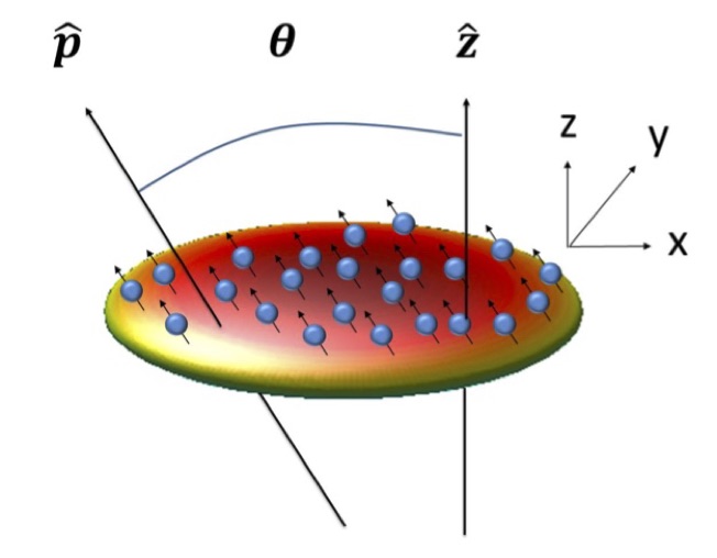
Figure 1: A dipolar BEC in the 2D “pancake” geometry, with the dipole moments $\mathbf{\hat{p}}$ oriented along the tilt angle defined, $\theta$, with respect to the normal axis, $\mathbf{\hat{z}}$.

II The effective 2D model

We consider an obliquely polarized dipolar BEC trapped in the pancake-shaped potential, as shown in Fig. 1. The oblique orientation of dipole moments is imposed by an external magnetic field, which makes the tilt angle, $\theta$, with the direction $\mathbf{\hat{z}}$ perpendicular to the pancake’s plane. The mean-field dynamics of the BEC at zero temperature is governed by by the GPE, which includes the integral term accounting for the DDI DDI-review :

$$i\hbar\frac{\partial\Psi(\mathbf{r},t)}{\partial t} = \left[-\frac{\hbar^{2}}{2m}\nabla^{2}+V(z)+g|\Psi(\mathbf{r},t)|^{2}\right.$$

$$+ \left.\left(\int d^{3}\mathbf{r}^{\prime}V_{d}(\mathbf{r}-\mathbf{r}^{\prime})|\Psi(\mathbf{r}^{\prime},t)|^{2}\right)\right]\Psi(\mathbf{r},t).$$

Here, $\Psi(\mathbf{r},t)$ is the wave function of condensate, $\mathbf{r}=(x,y,z)$ is the position vector, $m$ is the atomic mass, and $V(z)=m\omega_{z}^{2}{z}^{2}/2$ is the confining potential acting in the transverse direction. The anisotropic DDI kernel is

$$V_{d}(\mathbf{r})=g_{d}(1-3\cos^{2}\eta)/r^{3},$$ (2)

where the DDI strength is $g_{d}=\mu_{0}\mu_{m}^{2}/4\pi$, with the vacuum permeability $\mu_{0}$ and magnetic dipole moment $\mu_{m}$, while $\eta$ is the angle between vector $\mathbf{r}$ and the orientation of dipole moments $\mathbf{\hat{p}}$. Note that this kernel vanishes at $\eta=\arccos\left(1/\sqrt{3}\right)$, which coincides with the “magic angle” predicted by the VA as a boundary between stable and unstable solitons, see Eq. (19) below. The usual contact interaction is represented in Eq. (II) by the local cubic term with coefficient $g=4\pi\hbar^{2}a/m$, where $a$ is the $s$-wave scattering length $a$. The norm of the wave function is fixed by total number of atoms, $N=\int d^{3}\mathbf{r}|\Psi(\mathbf{r},t)|^{2}$.

The 3D GPE (II) can be reduced into an effective 2D equation, provided that the confinement in the $z$-direction is strong enough. To this end, we assume, as usual, that the 3D wave function is factorized, $\Psi(\mathbf{r})=\psi(\mathbf{\rho})\phi(z)\exp\left(-i\mu t/\hbar\right)$, with transverse coordinates $\mathbf{\rho}=(x,y)$ and chemical potential $\mu$ Luca ; Proukakis ; Luca2 . The transverse wave function is taken as the normalized ground state of the respective trapping potential, $\phi(z)=\left(\pi L_{z}^{2}\right)^{-1/4}\exp\left(-z^{2}/2L_{z}^{2}\right)$, with the characteristic length $L_{z}=\sqrt{\hbar/m\omega_{z}}$. Then, integrating Eq. (II) over the $z$-coordinate, the factorized ansatz leads one to the following effective 2D equation:

$$\left(\frac{\mu}{\hbar}-\frac{1}{2}\omega_{z}\right)\hbar\psi({\rho})=-\frac{\hbar^{2}}{2m}\nabla_{\perp}^{2}\psi(\rho)+\frac{g}{\sqrt{2\pi}L_{z}}|\psi(\rho)|^{2}\psi(\rho)$$

$$+\frac{g_{d}}{L_{z}}\left[\int\frac{d^{2}\mathbf{k}_{\rho}}{(2\pi)^{2}}\,n(\mathbf{k}_{\rho})V_{2d}\left(\frac{\mathbf{k}_{\rho}L_{z}}{\sqrt{2}}\right)\,e^{i\,\mathbf{k}_{\rho}\cdot\rho}\right]\psi(\rho),$$ (3)

where $\nabla_{\perp}^{2}\equiv\partial^{2}/\partial x^{2}+\partial^{2}/\partial y^{2}$, $n(\mathbf{k}_{\rho})\equiv\int d^{2}\rho\,|\psi(\rho)|^{2}\exp[-i\,\mathbf{k}_{\rho}\rho]$ is the Fourier transform of the 2D density, $|\psi(\rho)|^{2}$, and $k_{\rho}=(k_{x}^{2}+k_{y}^{2})^{1/2}$. Further, defining that the dipoles are polarized aligned in the $\left(x,z\right)$ plane, i.e., $\mathbf{\hat{p}}=(\sin\theta,0,\cos\theta)$ and $\cos\eta=\mathbf{\hat{p}}\cdot\hat{\mathbf{r}}$, in the momentum ($\mathbf{k}$-) space, the DDI kernel takes the form of

$$V_{2d}\left(\frac{\mathbf{k}_{\rho}L_{z}}{\sqrt{2}}\right)=-\frac{2\sqrt{2\pi}}{3}(1-3\cos^{2}\theta)$$ (4)

$$+\left[1-3\cos^{2}\theta+\cos(2\zeta)\sin^{2}\theta\right]\pi\mathbf{k}_{\rho}L_{z}\exp\left(\frac{\mathbf{k}_{\rho}^{2}L_{z}^{2}}{2}\right)$$

$$\times\text{erfc}\left(\frac{\mathbf{k}_{\rho}L_{z}}{\sqrt{2}}\right),$$

with $\cos\zeta\equiv k_{x}/k_{\rho}$ and the complementary error function erfc in the momentum space.

Rescaling Eq. (3) by $\mu\rightarrow\mu/\hbar\omega_{z}-1/2$, $\nabla_{\perp}\rightarrow\nabla_{\perp}L_{z}$, $\rho\rightarrow\rho/L_{z}$, $\mathbf{k}_{\rho}\rightarrow\mathbf{k}_{\rho}L_{z}$, $\psi(\rho)\rightarrow\psi(\rho)\sqrt{2(2\pi)^{1/2}|a|L_{z}}$, $g\rightarrow g/(4\pi\hbar\omega_{z}|a|L_{z}^{2})$, and $g_{d}\rightarrow g_{d}/(2\sqrt{2\pi}\hbar\omega_{z}|a|L_{z}^{2})$, we arrive at the following normalized 2D equation:

$$\mu\psi(\rho) = -\frac{1}{2}\nabla_{\perp}^{2}\psi(\rho)+g|\psi(\rho)|^{2}\psi(\rho)$$

$$+ g_{d}\left[\int\frac{d^{2}\mathbf{k}_{\rho}}{(2\pi)^{2}}\,n(\mathbf{k}_{\rho})V_{2d}\left(\frac{\mathbf{k}_{\rho}}{\sqrt{2}}\right)\,e^{i\,\mathbf{k}_{\rho}\cdot\rho}\right]\psi(\rho).$$

According to the rescaling, the norm of the 2D wave function, $N_{2}\equiv\int d^{2}\rho\,|\psi({\rho})|^{2}$, is related to the number of atoms: $N=N_{2}\times(L_{z}/(2\sqrt{2\pi}|a|)$.

Our model is based on Eq. (II). For example, in the case of the BECs of ⁵²Cr atoms, the atomic magnetic moment is $\mu_{m}=6$ $\mu_{\mathrm{Bohr}}$, and an experimentally relevant trapping frequency,

$$\omega_{z}=2\pi\times 800~{}\text{Hz}$$ (6)

Pfau-00 ; exp-Cr2 ; exp-Cr3 ; exp-Cr4 , corresponds to the characteristic transverse length $L_{z}=0.493$ $\mathrm{\mu}$m. With the same trapping frequency, for BECs of ¹⁶⁸Er atoms, we have $\mu_{m}=7$ $\mu_{\mathrm{Bohr}}$ and $m=2.8\times 10^{-25}$ gram, which corresponds to a characteristic transverse length $L_{z}=0.274$ $\mathrm{\mu}$m; while for ¹⁶²Dy atoms, we have $\mu_{m}=10$ $\mu_{\mathrm{Bohr}}$, $m=2.7\times 10^{-25}$ gram, and $L_{z}=0.279$ $\mathrm{\mu}$m, respectively.

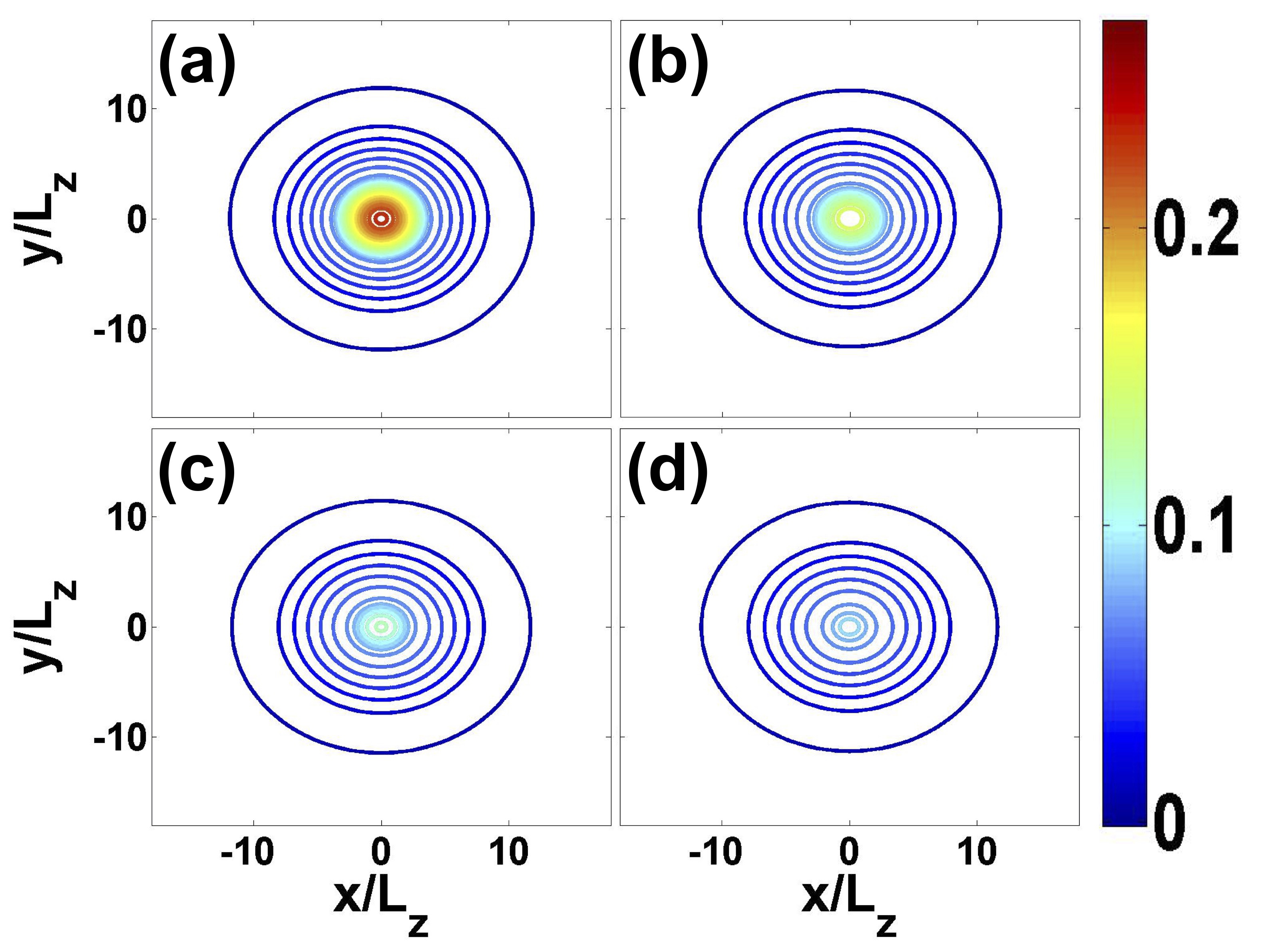
Figure 2: Transverse profiles of 2D solitons in the $x$-$y$ plane normalized to the characteristic transverse length $L_{z}$, by the produced by the numerical solution of Eq. (II), with chemical potential $\mu=-0.01$, fixed strength of contact attraction, $g=-1$, and a small DDI strength, $g_{d}=0.1$. The tilt angles are (a) $\theta=0$, (b) $\theta=0.73$ ($41.8^{\circ}$), (c) $\theta=\pi/3$, and (d) $\theta=\pi/2$. Here, the corresponding particle number $N_{2}$ are (a) $7.15$, (b) $6.23$, (c) $5.71$ and (d) $5.34$, respectively.

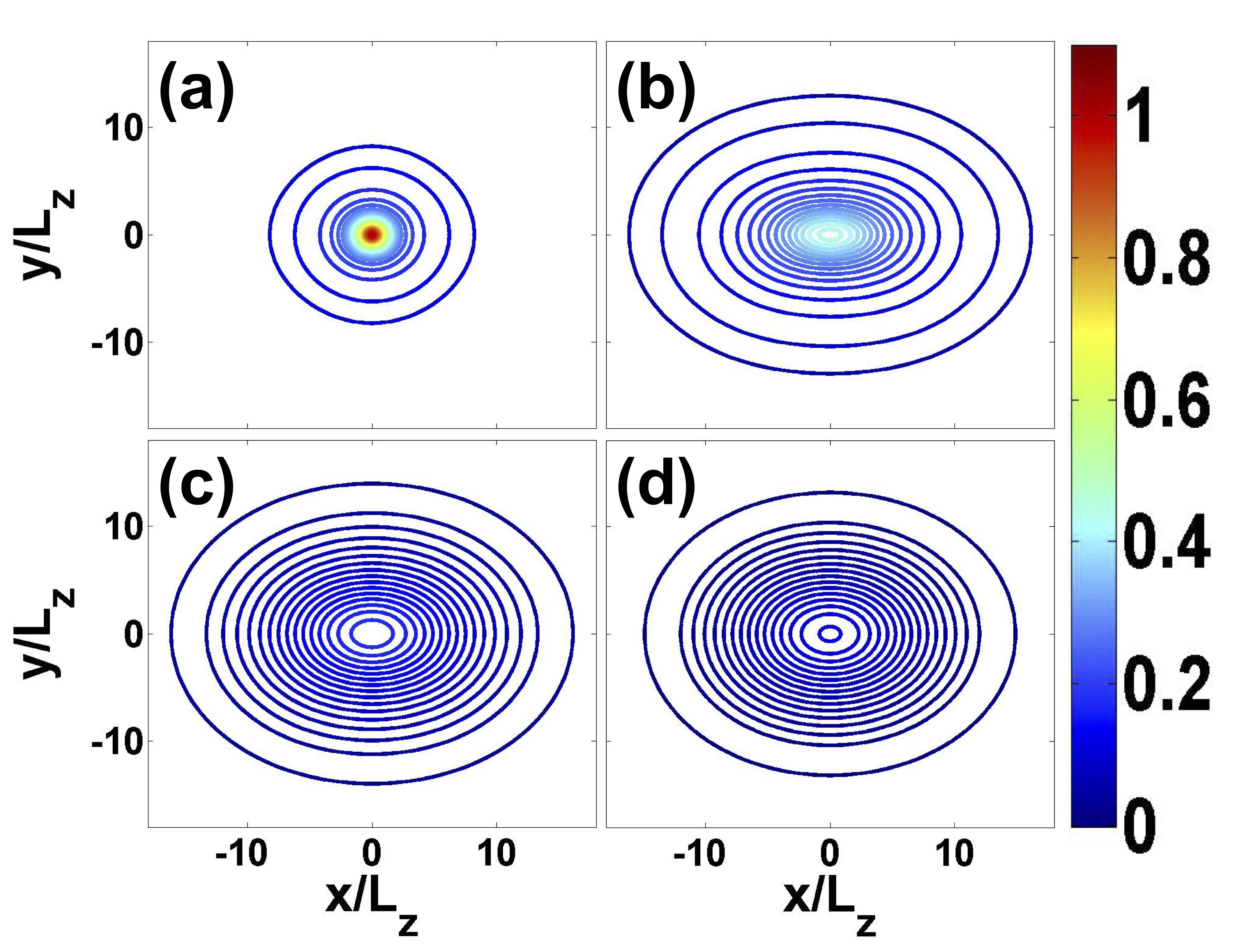
Figure 3: The same as in Fig. 2, but for stronger DDI, with $g_{d}=1.0$.Here, the corresponding particle number $N_{2}$ are (a) $4.69$, (b) $9.11$, (c) $4.53$, and (d) $2.86$, respectively.

II.1 2D numerical soliton solutions

In the absence of the DDI, $g_{d}=0$, solutions in the form of isotropic Townes solitons are supported by attractive contact interaction with $g<0$ Sulem ; Fibich ; soliton-book . Then, by fixing the strength of the contact attraction, $g=-1$, we introduce the DDI in Eq. (II) and seek for 2D bright-soliton solutions numerically, by varying the DDI strength, $g_{d}$, for different values of of the chemical potential, $\mu$. The validity of our effective 2D equation for the pancake geometry is ensured by checking that the transverse width of the 2D soliton solutions is larger than the transverse-confinement length, $L_{z}$ in the $z$-direction. This condition sets a constraint on the available range for the chemical potential, i.e., $|\mu|/\hbar\omega_{z}\ll 1$. In our simulations, the 2D effective equations remain valid in the range of

$$-0.1<\mu<-0.003.$$ (7)

The tilt angle of the dipoles in the $\left(x,z\right)$ plane was also varied, in the full interval of $0<\theta<\pi/2$. The DDI sign is fixed as $g_{d}>0$, which corresponds to the natural situation of the repulsion between the dipoles oriented perpendicular to the pancake’s plane, $\theta=0$. Thus, the DDI is isotropic but repulsive at $\theta=0$, being anisotropic at $\theta\neq 0$. Accordingly, the DDI tends to compete with the fixed-strength contact attraction.

Numerical solution of Eq. (II) produces 2D soliton profiles, typical examples of which are displayed in Figs. 2 and 3, for $\mu=-0.01$. With the fixed contact-interaction coefficient, $g=-1$, we find two different scenarios of the evolution of the shape of the 2D solitons. For weak DDI, such as with coefficient $g_{d}=0.1$, starting with the isotropic profile at $\theta=0$ [Fig. 2(a)], the transverse widths in $x$- and $y$-directions both expand, but at different rates, as the tilt angle increases, see Fig. 2(b-d) for $\theta=0.73$ ($41.8^{\circ}$) and $\pi/3$, respectively. The 2D solitons are wider along the $x$-direction and narrower along $y$ because the dipoles are tilted in the $\left(x,z\right)$ plane.

For a larger DDI strength, such as $g_{d}=1.0$, we still have an isotropic profile at $\theta=0$, as shown in Fig. 3(a). As the tilt angle increases, the transverse widths in $x$- and $y$-directions shrink just slightly, remaining nearly equal at $\theta=0.73$ ($41.8^{\circ}$), $\pi/3$, and $\pi/2$, as shown in Figs. 3(b-d). Note that, quite naturally, the radius of the isotropic profile, observed at $\theta=0$, is smaller in Fig. 2(a) than in Fig. 3(a), as in the latter case the dipole-dipole repulsion is much stronger than the competing contact attraction. Nevertheless, the increase of $\theta$ makes the expansion of the profiles and the growth of its anisotropy, which are effects of the DDI, more salient in Fig. 2, i.e., when the DDI is weaker. This counter-intuitive evolution of the shape may be explained by the fact that it is shown not for the fixed number of atoms, $N_{2}$, but for a fixed chemical potential, $\mu$. To keep the same $\mu$ in the case of the stronger DDI competing with the contact self-attraction (in Fig. 3), the system needs to increase $N_{2}$, which, in turn, helps the contact interaction to keep the compact nearly-isotropic shape of the soliton.

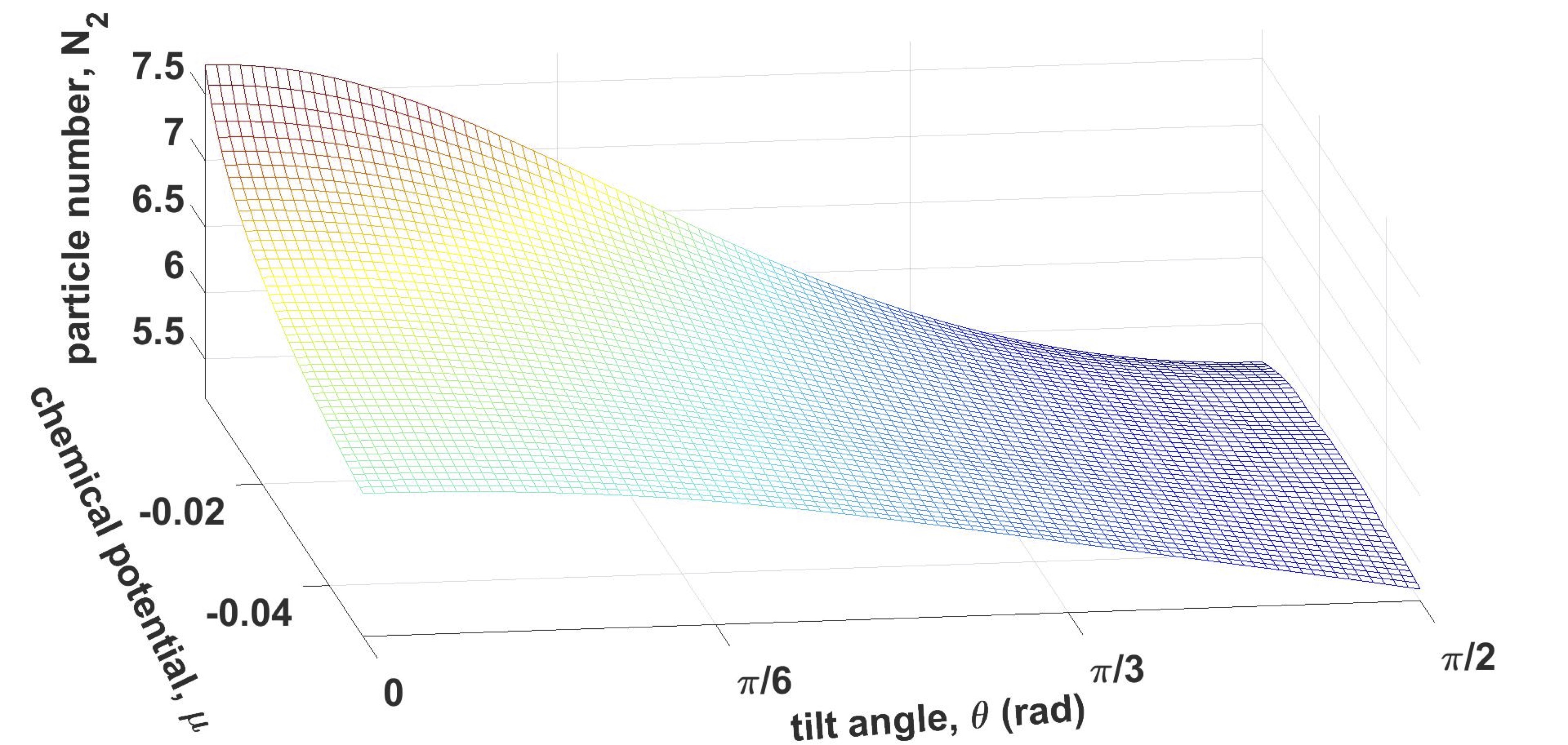
Figure 4: The scaled 2D particle number, $N_{2}$ in the soliton solutions,versus the tilt angle, $\theta$, and chemical potential, $\mu$, at the fixed strength of the contact interaction, $g=-1$, and a small DDI strength, $g_{d}=0.1$.

.

Figure 5: The same as in Fig. 4, but for a much stronger DDI, with $g_{d}=1.0$. In this case, $N_{2}$ attains ist maximum at $\theta\approx 0.73$ ($41.8^{\circ}$), irrespective of the value of $\mu$.

To present a clearer illustration on these trends, we display, in Figs. 4 and 5, $N_{2}$ as a function of $\theta$ and $\mu$, for the same small and large strengths of DDI, i.e., $g_{d}=0.1$ and $g_{d}=1.0$, respectively. In accordance with what is said above, $N_{2}$ decreases monotonously at $g_{d}=0.1$, as the tilt angle increases from $\theta=0$ to $\pi/2$, at all values of $\mu$. However, the stronger DDI strength (with $g_{d}=1.0$) produces a completely different picture (also in agreement with the above explanation): as $\theta$ increases from $0$, $N_{2}$ at first increases too, reaching a maximum at

$$\theta=\theta_{0}\approx 0.73~{}(\text{equivalent to }41.8^{\circ})$$ (8)

[note that this angle is smaller than the critical (“magic”) one, $\theta_{m}$, given below by Eq. (19), which is an approximate boundary between the stable and unstable solitons]. As mentioned above, the increase of $N_{2}$ is necessary to keep the same value of $\mu$ while the essentially repulsive DDI competes with the local self-attraction, at $\theta<\theta_{0}$. Then, $N_{2}$ decreases, as $\theta$ passes $\theta_{0}$ and approaches $\pi/2$. Indeed, in the latter case, the DDI becomes essentially attractive anisotropic-soliton , hence the local and nonlocal interaction act together, instead of competing, making it possible to keep the given value of $\mu$ with a smaller norm. Note that these trends are the same at different values of $\mu$, although the corresponding values of $N_{2}$ are, naturally, different. Below, we demonstrate that angle $\theta_{0}$ can be accurately predicted by the variational approximation, see Fig. 6(a).

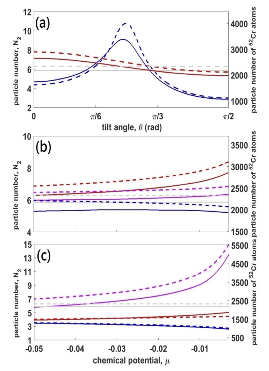
Figure 6: Comparison of the norm of the 2D wave function, $N_{2}$, as produced by tne numerical solution and variational approximation (solid and dashed lines, respectively). (a) $N_{2}(\theta)$ at fixed $\mu=-0.01$, for the weak and strong DDI, $g_{d}=0.1$ and $1$ (red and blue lines, respectively). Two other panels display $N_{2}(\mu)$ for the same fixed values of the DDI strength: $g_{d}=0.1$ (b) and $1.0$ (c). In these panels, fixed values of the tilt angle are $\theta=0$ (red lines), $\theta=\theta_{0}\approx 0.73$ [see Eq. (8); magenta], and $\theta=\pi/2$ (blue). In each panel we also show, by solid and dashed black horizontal lines, the constant value of $N_{2}$ for the Townes soliton (when the DDI is absent, $g_{d}=0$) and its variationally predicted counterpart (see the main text for details). For the condensate of ⁵²Cr atoms, the corresponding total numbers of atoms, for fixed values of other parameters [see Eq. (6)], are given on the right vertical axes, as a reference for a possible experiment.

II.2 The variational approximation (VA)

In addition to numerical solutions, we have developed the VA, following the lines of Refs. variation-1 ; variation and using the Lagrangian density corresponds to Eq. (II)

$$\mathcal{L} = -\mu|\psi|^{2}+\frac{1}{2}|\nabla_{\perp}\psi|^{2}+\frac{g}{2}|\psi|^{4}$$ (9)

$$+ \frac{g_{d}}{2}|\psi|^{2}\int d^{2}\rho^{\prime}\,V_{2d}\left(\rho-\rho^{\prime}\right)|\psi(\rho^{\prime})|^{2}.$$

The corresponding Gaussian ansatz is, naturally, anisotropic:

$$\psi_{\text{ans}}=\sqrt{\frac{N_{2}}{\pi w_{x}w_{y}}}\exp\left(-\frac{x^{2}}{2w_{x}^{2}}-\frac{y^{2}}{2w_{y}^{2}}\right)\,,$$ (10)

with the 2D norm $N_{2}$, and different transverse widths in $x$- and $y$-directions, $w_{x}$ and $w_{y}$. Then, the effective Lagrangian $L=\int dxdy\,\mathcal{L}$ is calculated:

$$L = -N_{2}\mu+\frac{N_{2}(w_{x}^{2}+w_{y}^{2})}{4w_{x}^{2}w_{y}^{2}}$$ (11)

$$+ \frac{gN_{2}^{2}}{4\pi w_{x}w_{y}}+\frac{g_{d}N_{2}^{2}}{8\pi^{2}}\left(f_{1}+f_{2}\right),$$

were we have introduced the short-hand notation:

$$f_{1}=-\frac{4\sqrt{2}\pi^{3/2}}{3w_{x}w_{y}}\left(1-3\cos^{2}\theta\right),$$

$$f_{2}=2\pi^{2}\int_{0}^{\infty}dk_{\rho}\,\left\{k_{\rho}^{2}\exp\left(\frac{2k_{\rho}^{2}-k_{\rho}^{2}(w_{x}^{2}+w_{y}^{2})}{4}\right)\right.$$

$$\times\text{erfc}\left(\frac{k_{\rho}}{\sqrt{2}}\right)\times\left[(1-3\cos^{2}\theta)\,I_{0}\left(\frac{k_{\rho}^{2}(w_{x}^{2}-w_{y}^{2})}{4}\right)\right.$$

$$\left.\left.-\left(\sin^{2}\theta\right)\,I_{1}\left(\frac{k_{\rho}^{2}(w_{x}^{2}-w_{y}^{2})}{4}\right)\right]\right\},$$ (12)

with the modified Bessel functions, $I_{0,1}\left(z\right)$. The Euler-Lagrange equations follow from Eq. (11) in the form of $\partial L/\partial\left(w_{x,y},N_{2}\right)=0$:

$$-\mu+\frac{w_{x}^{2}+w_{y}^{2}}{4w_{x}^{2}w_{y}^{2}}+\frac{gN_{2}}{2\pi w_{x}w_{y}}+\frac{g_{d}N_{2}(f_{1}+f_{2})}{4\pi^{2}}=0,$$ (13)

$$-\frac{1}{2w_{x}^{3}}-\frac{gN_{2}}{4\pi w_{x}^{2}w_{y}}+\frac{g_{d}N_{2}}{8\pi^{2}}\left(\frac{\partial{f_{1}}}{\partial{w_{x}}}+\frac{\partial{f_{2}}}{\partial{w_{x}}}\right)=0,$$ (14)

$$-\frac{1}{2w_{y}^{3}}-\frac{gN_{2}}{4\pi w_{x}w_{y}^{2}}+\frac{g_{d}N_{2}}{8\pi^{2}}\left(\frac{\partial{f_{1}}}{\partial{w_{y}}}+\frac{\partial{f_{2}}}{\partial{w_{y}}}\right)=0.$$ (15)

For small arguments, $0<|z|\ll\sqrt{\alpha+1}$, the modified Bessel function can be replaced by the first term of its expansion, $I_{\alpha}(z)\approx(z/2)^{\alpha}/\Gamma(\alpha+1)$, where $\Gamma$ is the Gamma-function. Such an approximation makes it possible to simplify Eqs. (13)-(15) in the case of

$$0<k_{\rho}^{2}(w_{x}^{2}-w_{y}^{2})/4\ll 1.$$ (16)

This condition implies that either the soliton is wide in comparison with the characteristic transverse-confinement width, $L_{z}$ (which may be naturally expected from the quasi-2D solitons), i.e., $k_{\rho}\ll 1$, or the profile is an almost symmetric one, with $\left|w_{x}^{2}-w_{y}^{2}\right|\ll w_{x,y}^{2}$. Further analysis makes it possible to expand, under condition (16) and to the first-order in $g_{d}$, the VA-predicted 2D norm of the wave function as

$$N_{2}(\mu)=2\pi-\frac{g_{d}\,\pi^{3/2}[1+3\cos(2\theta)]}{3(1+2\mu)^{2}\sqrt{\frac{-2}{\mu}-4}}\times$$ (17)

$$\left[(4+2\mu)(4\mu-1)\sqrt{\frac{-1}{\mu}-2}+9\sqrt{2}\arctan\sqrt{\frac{-1}{2\mu}-1}\right],$$

where $2\pi$ is the well-known VA prediction for the 2D norm of the Townes solitons variation-1 , which is obviously valid in the limit of $g_{d}=0$, while the term $\sim g_{d}$ in Eq. (17) is a small correction to it. The correction is a critically important one, as it lifts the degeneracy of the Townes solitons, whose norm does not depend on $\mu$ Townes ; Sulem ; Fibich , and thus makes it possible to check the VK criterion, which states that a necessary condition for the stability of any soliton family supported by self-attractive nonlinearity is $dN_{2}/d\mu<0$ VK ; vk1 ; vk2 ; vk3 . It originates from the condition that a soliton which may be stable should realize a minimum of the energy for a given value of the norm. Note also that condition $-1/2<\mu<0$, which is obviously necessary for the validity of Eq. (17), definitely holds in the range of $\mu$ given by Eq. (7), dealt with in the present work.

Applying the VK criterion to the $N_{2}(\mu)$ dependence given by Eq. (17), we obtain

$$\frac{d\,N_{2}}{d\,\mu}=-\frac{\,g_{d}\pi^{3/2}\left(1-3\cos^{2}\theta\right)}{\mu(1+2\mu)^{3}\sqrt{\frac{-2}{\mu}-4}}$$ (18)

$$\times\left[2\mu(4\mu-13)\sqrt{\frac{-1}{\mu}-2}+3\sqrt{2}(8\mu-1)\tan^{-1}\sqrt{\frac{-1}{2\mu}-1}\right].$$

It immediately follows from Eq. (18) that the VK criterion holds, i.e., the solitons may be stable (in the framework of the VA), if the dipoles are polarized under a sufficiently large angle $\theta$ with respect to the normal direction, i.e., the polarization is relatively close to the in-plane configuration (cf. Ref. anisotropic-soliton ):

$$\theta>\theta_{m}\equiv\cos^{-1}(1/\sqrt{3})\approx 0.955~{}(\text{tantamount to }54.74^{\circ}).$$ (19)

On the other hand, the solitons are predicted to be definitely unstable at $\theta<\theta_{m}$. The same critical (alias “magic”) angle is known, e.g., in the theory of the nuclear magnetic resonance, when a sample is spinning about a fixed axis magic-1 ; magic-2 . Note that, in the framework of the approximation based on Eqs. (17) and (18), at $\theta=\theta_{m}$ the 2D norm of the solitons coincides with that of the Townes solitons.

In the more general case, we have found the VA-predicted parameters $N_{2}$ and $w_{x,y}$ solving Eqs. (13)-(15) numerically. In Fig.. 6 we present the comparison of norm of $N_{2}$, as obtained from the full numerical solution of Eq. (II) and its counterpart predicted by the VA (solid and dashed curves, respectively). For the reference, we also show the constant value, $N_{2}^{(T)}\approx 5.85$ for the Townes solitons ($g_{d}=0$), and its above-mentioned VA-predicted counterpart, $N_{2}^{(T)}=2\pi$ variation-1 . In particular, Fig. 6(a) features the same trends in the dependence $N_{2}(\theta)$ at fixed $\mu$ as were identified, and qualitatively explained, above while addressing Figs. 4 and 5: in the case of the weak DDI, the dependence is monotonous, while the strong DDI gives rise to a well-pronounced maximum at point (8).

In Fig. 6, we also depict the 2D norm $N_{2}$ as a function of the chemical potential, $\mu$, for (b) weak and (c) strong DDI, i.e., $g_{d}=0.1$ and $1.0$, respectively, for three fixed tilt angles, namely, $\theta=0$ (the dipoles polarized perpendicular to the pancake), $\theta=\theta_{0}$ [the special value given by Eq. (8)], and $\theta=\pi/2$ (the in-plane polarization). In particular, it is seen that the slope of the $N_{2}\left(\mu\right)$ dependences, which determines the VK criterion, is definitely positive, slightly or strongly positive (for small or large DDI strength), and slightly negative, for $\theta=0$ (red curves), $\theta=\theta_{0}$ (magenta curves), and $\theta=\pi/2$ (blue curves), respectively. These conclusions, which pertain to the weak and strong DDI alike, agree with the prediction of Eq. (18), namely, $dN_{2}/d\mu<0$ for $\theta>\theta_{m}$, and $dN_{2}/d\mu>0$ for $\theta<\theta_{m}$.

Lastly, Figs. 6(b,c) also show, as a reference for possible experimental realization, the expected numbers of atoms in the solitons created in the ⁵²Cr condensate, transversely trapped under condition (6).

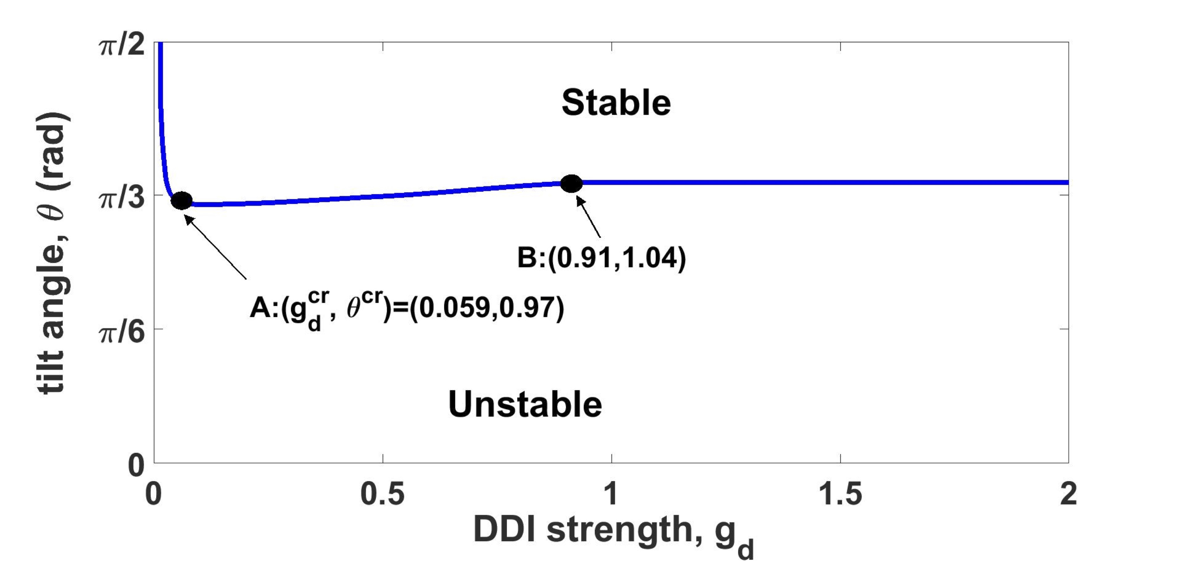
Figure 7: The stability map for 2D solitons in the plane of the DDI strength, $g_{d}$, and the tilt angle, $\theta$, as produced by the solution of the eigenvalue problem for small perturbations. The solitons are stable at $\theta^{\text{cr}}<\theta\leq\pi/2$, where $\theta^{\text{cr}}(g_{d})$ is shown by the blue line. As above, the strength of the contact interaction is fixed to be $g=-1$. Points A and B correspond, respectively, to the smallest and largest values of $\theta^{\text{cr}}$, respectively (the definition of the largest value excludes the narrow stripe of the quick decrease of $\theta^{\text{cr}}$ with the increase of $g_{d}$ from $0$ to point A). In fact, the difference between the largest and smallest values is small. The nearly flat shape of the stability boundary roughly agrees with the analytical prediction given by Eq. (19).

III Stability of the 2D solitons

As said above, stability is the critically important issue for 2D solitons, as the usual cubic local self-attraction creates Townes solitons which are subject to the subexponential instability against small perturbations BAMalomed ; Sulem ; Fibich . Originally, the perturbations grow with time algebraically, rather than exponentially, but eventually the solitons are quickly destroyed. The subexponential instability implies that, in terms if the above-mentioned VK criterion, the Townes solitons are, formally, neutrally stable, having $dN_{2}/d\mu=0$ [see the flat black lines in Figs. 6(b,c)].

As said above, Eq. (18) and Figs. 6(b,c) demonstrate that the addition of the DDI to the local self-attraction lifts the degeneracy (the independence of the norm of the Townes solitons on the chemical potential). The resulting sign of the slope, $dN_{2}/d\mu$, is the same for the numerical solutions and their counterparts predicted by the variational approximation. The sign is the same too for both the weak and strong DDI ($g_{d}=0.1$ and $g_{d}=1$). Equation (18) produces an important prediction, that, with the increase of the title angle from $\theta=0$ to $\pi/2$, the slope $dN_{2}/d\mu$ changes from positive (unstable) to negative (possibly stable) at the “magic angle” given by Eq. (19).

Because the VK criterion is only a necessary stability condition, and also because Eq. (18) was derived in approximately, under condition Eq. (16), it is necessary to develop the consistent linear stability analysis for our numerically generated soliton solutions. To this end, we introduce a perturbed solution as

$$\psi(\rho,t)=\{\psi_{0}(\rho)+\epsilon\left[p(\rho)e^{-i\delta t}+q(\rho)e^{i\delta^{\ast}t}\right]\}e^{-i\mu t}.$$ (20)

Here, the asterisk stands for the complex-conjugate value, $\psi_{0}(\rho)$ is the unperturbed solution, $\epsilon$ is an infinitesimal perturbation amplitude, while $p(\rho)$ and $q(\rho)$ are eigenmodes of the small perturbation, with the respective eigenvalue $\delta$. The instability occurs in the case when $\delta$ is not real. The unperturbed solution was classified as a stable one if the numerically found instability growth rate, $\left|\mathrm{Im}(\delta)\right|$, was smaller than $10^{-7}$.

Results of the stability analysis are summarized in Fig. 7, where the stability map for the soliton solutions is displayed in the plane of the DDI strength, $g_{d}$, and the tilt angle, $\theta$, the stability region being

$$\theta^{\mathrm{cr}}(g_{d})<\theta\leq\pi/2.$$ (21)

This map is found to be the same, up to the accuracy of the numerically collected data, for the entire interval (7) of values of the chemical potential in which the derivation of the effective 2D equation (II) is valid. This map shows that the originally unstable Townes solitons, corresponding to $g_{d}=0$, quickly attains the stability saturation, i.e., expansion of the stability interval (21) to its limits, $\theta^{\mathrm{cr}}\approx\theta_{m}<\theta\leq\pi/2$, at very small values of $g_{d}$. At $g_{d}=g_{d}^{\text{cr}}\approx 0.059$, the stability boundary attains its minimum value, $\theta^{\text{cr}}\approx 0.97$, as labeled by the point A in Fig. 7. With the increase of $g_{d}$, the critical tilt slightly increases to $\theta=1.04$ (tantamount to $59.59^{\circ}$), as labeled by point B, which corresponds to $g_{d}=0.91$. Comparing these numerically exact results with the analytical prediction given by Eq. (19), we conclude that the relative error is limited to $8.2\%$, and, although the VA fails to predict the dependence of $\theta^{\text{cr}}$ on $g_{d}$, the actual dependence is quite weak.

Lastly, it is relevant to stress that, setting $dN_{2}/d\mu=0$ to identify the VK-predicted stability boundary, we obtain results, from the full numerical solution, for both weak and strong DDI, with $g_{d}=0.1$ and $1.0$, respectively, which exactly coincide with the stability boundary identified above through the calculation of the linear-stability eigenvalues, i.e., $\theta^{\text{cr}}=0.97$ and $1.04$.

Before the conclusion, we discuss the possibility to stabilize dipolar BECs with quantum fluctuations. The stability boundary we reveal above is based on the mean-field theory. However, when the quantum fluctuations are taken into consideration, a repulsive, known as Lee-Huang-Yang (LHY), correction may stabilize an attractive Bose gas 65 . Recently, experimental observations on stable and ordered arrangement of droplets in an atomic dysprosium BEC illustrated the importance of LHY quantum fluctuations in stabilizing the system against collapse 66 ; 67 . LHY corrections have be shown to stabilize droplets in unstable Bose-Bose mixtures 68 , and self-bound filament-like droplets 69 . Relations on an arbitrary tilt angle to LHY corrections, and related stability of 2D solitons with DDI interaction deserve further study.

IV Conclusion

For the dipolar BEC confined to the pancake geometry, we have investigated the formation and stability of 2D soliton with the atomic magnetic moments polarized in an arbitrary direction. Fixing the strength of contact attractive interaction (which, by itself, would only create unstable Townes solitons), we demonstrate, by means of the numerical methods and VA (variational approximation), combined with the VK (Vakhitov-Kolokolov) criterion, that the 2D solitons can be completely stabilized by the DDI (dipole-dipole interaction) with relative strength $g_{d}$, which makes the solitons anisotropic. Both the VK criterion and numerically exact linear-stability analysis confirm that, there exists a “magic angle” of the polarization tilt, $\theta^{\text{cr}}$, such that the 2D solitons are stable at $\theta^{\mathrm{cr}}(g_{d})<\theta\leq\pi/2$. While the VA predicts $\theta^{\mathrm{cr}}=\arccos(1/\sqrt{3})$ which does not depend on $g_{d}$, the numerically exact results feature a weak dependence of $\theta^{\mathrm{cr}}$ on $g_{d}$, with the actual values of $\theta^{\mathrm{cr}}$ being quite close to the VA prediction. We also produce physical parameters for experiments in the condensate of ⁵²Cr atoms, which should make the creation of the stable 2D solitons possible.

References

- (1) C. J. Pethick and H. Smith, “Bose-Einstein Condensation in Dilute Gases,” (Cambridge University Press, 2008).
- (2) B.A. Malomed, D. Mihalache, F. Wise, and L. Torner, “Spatiotemporal optical solitons,” J. Opt. B: Quantum Semiclass. Opt. 7, R53 (2005); “Viewpoint: On multidimensional solitons and their legacy in contemporary Atomic, Molecular and Optical physics”, J. Phys. B: At. Mol. Opt. Phys. 49, 170502 (2016).
- (3) D. Mihalache, “Linear and nonlinear light bullets: Recent theoretical and experimental studies”, Rom. J. Phys. 57, 352-371 (2012).
- (4) B. A. Malomed, “Multidimensional solitons: Well-established results and novel findings”, Eur. Phys. J. Special Topics 225, 2507-2532 (2016).
- (5) R. Y. Chiao, E. Garmire, and C. H. Townes, “Self-Trapping of Optical Beams,” Phys. Rev. Lett. 13, 479 (1964).
- (6) C. Sulem and P. L. Sulem, The nonlinear Schrödinger equation: self-focusing and wave collapse (Springer: Berlin, 1999).
- (7) G. Fibich, The Nonlinear Schrödinger Equation: Singular Solutions and Optical Collapse (Springer, Heidelberg, 2015)
- (8) A. Posazhennikova, “Weakly interacting, dilute Bose gases in 2D,” Rev. Mod. Phys. 78, 1111 (2006).
- (9) A. Griesmaier, J. Werner, S. Hensler, J. Stuhler, and T. Pfau, “Bose-Einstein Condensation of Chromium,” Phys. Rev. Lett. 94, 160401 (2005).
- (10) M. Lu, N. Q. Burdick, S. H. Youn, and B. L. Lev, “Strongly Dipolar Bose-Einstein Condensate of Dysprosium,” Phys. Rev. Lett. 107, 190401 (2011).
- (11) K. Aikawa, A. Frish, M. Mark, S. Baier, A. Rietzler, R. Grimm, and F. Ferlaino “Bose-Einstein Condensation of Erbium,” Phys. Rev. Lett. 108, 210401 (2012).
- (12) A. Griesmaier, “Generation of a dipolar Bose–Einstein condensate”, J. Phys. B: At. Mol. Opt. Phys. 40, R91-R134 (2007).
- (13) T. Lahaye, C. Menotti, L. Santos, M. Lewenstein, and T. Pfau, “The physics of dipolar bosonic quantum gases”, Rep. Prog. Phys. 72, 126401 (2009).
- (14) A. W. Synder and D. J. Mitchell, “Accessible Solitons,” Science 276, 1538 (1997).
- (15) G. Assanto and M. Peccianti, “Spatial solitons in nematic liquid crystals”, IEEE J. Quant. Elect. 39, 13-21 (2003).
- (16) C. Conti, M. Peccianti, and G. Assanto, “Observation of optical spatial solitons in a highly nonlocal medium”, Phys. Rev. Lett. 92, 113902 (2004).
- (17) W. Krolikowski, O. Bang, N. I. Nikolov, D. Neshev, J. Wyller, J. J. Rasmussen, and D. Edmundson, “Modulational instability, solitons and beam propagation in spatially nonlocal nonlinear media,” J. Opt. B: Quantum. Semiclass. Opt. 6, S288 (2004).
- (18) Y. V. Kartashov, V. A. Vysloukh, and L. Torner, “Tunable soliton self-bending in optical lattices with nonlocal nonlinearity,” Phys. Rev. Lett. 93, 153903 (2004).
- (19) Z. Xu, Y. V. Kartashov, and L. Torner, “Soliton Mobility in Nonlocal Optical Lattices,” Phys. Rev. Lett. 95, 113901 (2005).
- (20) G. Gligorić, A. Maluckov, L. Hadžievski, and B. A. Malomed, “Bright solitons in the one-dimensional discrete Gross-Pitaevskii equation with dipole-dipole interactions”, Phys. Rev. A 78, 063615 (2008).
- (21) G. Gligorić, A. Maluckov, M. Stepić, L. Hadžievski, and B. A. Malomed, “Two-dimensional discrete solitons in dipolar Bose-Einstein condensates”, Phys. Rev. A 81, 013633 (2010).
- (22) S. Lopez-Aguayo, A. S. Desyatnikov, Yu. S. Kivshar, S. Skupin, W. Krolikowski, and O. Bang, “Stable rotating dipole solitons in nonlocal optical media,” Opt. Lett. 31, 1100 (2006).
- (23) D. Briedis, D. E. Petersen, D. Edmundson, W. Krolikowski, O. Bang, “Ring vortex solitons in nonlocal nonlinear media,” Opt. Exp. 13, 435 (2005).
- (24) C. Rotschild, O. Cohen, O. Manela, M. Segev, and T. Carmon, “Solitons in nonlinear media with an infinite range of nonlocality: First observation of coherent elliptic solitons and of vortex-ring solitons,” Phys. Rev. Lett. 95, 213904 (2005).
- (25) D. Buccoliero, A. S. Desyatnikov, W. Krolikowski, and Yu. S. Kivshar, “Laguerre and Hermite soliton clusters in nonlocal nonlinear media,” Phys. Rev. Lett. 98, 053901 (2007).
- (26) Y. V. Kartashov, L. Torner, V. A. Vysloukh, and D. Mihalache, “Multipole vector solitons in nonlocal nonlinear media,” Opt. Lett. 31, 1483 (2006).
- (27) A. Alberucci, M. Peccianti, G. Assanto, A. Dyadyusha, and M. Kaczmarek, “Two-color vector solitons in nonlocal media,” Phys. Rev. Lett. 97 153903 (2006).
- (28) Y. Lin, and R.-K. Lee, “Dark-bright soliton pairs in nonlocal nonlinear media,” Opt. Exp. 15, 8781 (2007).
- (29) S. K. Adhikari, “Stable, mobile, dark-in-bright, dipolar Bose-Einstein-condensate solitons,” Phys. Rev. A 89, 043615 (2014).
- (30) S. Yi and L. You, “Trapped condensates of atoms with dipole interactions,” Phys. Rev. A 63, 053607 (2001).
- (31) L. Santos, G. V. Shlyapnikov, and M. Lewenstein, “Roton-Maxon Spectrum and Stability of Trapped Dipolar Bose-Einstein Condensates,” Phys. Rev. Lett. 90, 250403 (2003).
- (32) R. Nath, P. Pedri, and L. Santos, “Phonon Instability with Respect to Soliton Formation in Two-Dimensional Dipolar Bose-Einstein Condensates,” Phys. Rev. Lett. 102, 050401 (2009).
- (33) A. D. Martin and P. B. Blakie, “Stability and structure of an anisotropically trapped dipolar Bose-Einstein condensate: Angular and linear rotons,” Phys. Rev. A 86, 053623 (2012).
- (34) R. K. Kumar, P. Muruganandam and B. A. Malomed, “Vortical and fundamental solitons in dipolar Bose-Einstein condensates trapped in isotropic and anisotropic nonlinear potentials,” J. Phys. B: At. Mol. Opt. Phys. 46, 175302 (2013).
- (35) C. Mishra and R. Nash, “Dipolar condensates with tilted dipoles in a pancake-shaped confinement,” Phys. Rev. A 94, 033633 (2016).
- (36) P. Pedri and L. Santos, “Two-dimensional bright solitons in dipolar Bose-Einstein condensates,” Phys. Rev. Lett. 95, 200404 (2005).
- (37) C. Eberlein, S. Giovanazzi, and D. H. J. O’Dell, “Exact solution of the Thomas-Fermi equation for a trapped Bose-Einstein condensate with dipole-dipole interactions,” Phys. Rev. A 71, 033618 (2005).
- (38) U. R. Fischer, Phys. Rev. A 73, “Stability of quasi-two-dimensional Bose-Einstein condensates with dominant dipole-dipole interactions,” 031602 (2006).
- (39) D. C. E. Bortolotti, S. Ronen, J. L. Bohn, and D. Blume, “Scattering Length Instability in Dipolar Bose-Einstein Condensates,” Phys. Rev. Lett. 97, 160402 (2006).
- (40) Y. Y. Lin, R.-K. Lee, Y.-M. Kao and T.-F. Jiang, “Band structures of a dipolar Bose-Einstein condensate in one-dimensional lattices,” Phys. Rev. A 78, 023629 (2008).
- (41) J. Cuevas, B. A. Malomed, P. G. Kevrekidis, and D. J. Frantzeskakis, “Solitons in quasi-one-dimensional Bose-Einstein condensates with competing dipolar and local interactions,” Phys. Rev. A 79, 053608 (2009).
- (42) K. Lakomy, R. Nath, and L. Santos, “Soliton molecules in dipolar Bose-Einstein condensates,” Phys. Rev. A 86, 013610 (2012).
- (43) A. J. Olson, D. L. Whitenack and Y. P. Chen, “Effects of magnetic dipole-dipole interactions in atomic Bose-Einstein condensates with tunable -wave interactions,” Phys. Rev. A 88, 043609 (2013).
- (44) S. Ronen, D. C. E. Bortolotti, and J. L. Bohn, “Radial and Angular Rotons in Trapped Dipolar Gases,” Phys. Rev. Lett. 98, 030406 (2007).
- (45) P. B. Blakie, D. Baillie, and R. N. Bisset, “Roton spectroscopy in a harmonically trapped dipolar Bose-Einstein condensate,” Phys. Rev. A 86, 021604 (2012).
- (46) I. Tikhonenkov, B. A. Malomed, and A. Vardi, “Anisotropic soliton in Dipolar Bose-Einstein Condensate,” Phys. Rev. Lett. 100, 090406 (2008).
- (47) P. Köberle, D. Zajec, G. Wunner, and B. A. Malomed, “Creating two-dimensional bright solitons in dipolar Bose-Einstein condensates”, Phys. Rev. A 85, 023630 (2012).
- (48) N. G. Vakhitov and A. A. Kolokolov, “Stationary solutions of the wave equation in the medium with nonlinearity saturation,” Radiophys. Quant. Electron. 16, 783 (1973).
- (49) E. R. Andrew, A. Bradbury, and R. G. Eades, “Nuclear magnetic resonance spectra from a crystal rotated at high speed,” Nature 182, 1659 (1958).
- (50) I. J. Lowe, “Free Induction Decays of Rotating Solids,” Phys. Rev. Lett. 2, 285 (1959).
- (51) L. Salasnich, A. Parola, and L. Reatto, “Condensate bright solitons under transverse confinement”, Phys. Rev. A 65, 043614 (2002), Phys. Rev. A 66, 043603 (2002).
- (52) U. Al Khawaja, J. O. Andersen, N. P. Proukakis, and H. T. C. Stoof, “Low dimensional Bose gases”, Phys. Rev. A 66, 013615 (2002).
- (53) L. Salasnich and B. A. Malomed, “Solitons and solitary vortices in pancake-shaped Bose-Einstein condensates”, Phys. Rev. A 79, 053620 (2009).
- (54) K. Goral, K. Rzazewski, and T. Pfau, “Bose-Einstein condensation with magnetic dipole-dipole forces,” Phys. Rev. A 61, 051601 (2000).
- (55) J. Werner, A. Griesmaier, S. Hensler, J. Stuhler, T. Pfau, A. Simoni and E. Tiesinga, “Observation of Feshbach Resonances in an Ultracold Gas of 52Cr,” Phys. Rev. Lett. 94, 183201 (2005).
- (56) J. Stuhler, A. Griesmaier, T. Koch, M. Fattori, T. Pfau, S. Giovanazzi, P. Pedri, and L. Santos, “Observation of Dipole-Dipole Interaction in a Degenerate Quantum Gas,” Phys. Rev. Lett. 95, 150406 (2005).
- (57) A. Griesmaier, J. Stuhler, and T. Pfau, “Production of a chromium Bose-Einstein condensate”, Appl. Phys. B 82, 211 (2006).
- (58) Yu. S. Kivshar and G. P. Agrawal, Optical Solitons: from Fibers to Photonic Crystals, (Academic: San Diego, 2003).
- (59) M. Desaix, D. Anderson, and M. Lisak, “Variational approach to collapse of optical pulses,” J. Opt. Soc. Am. B 8, 2082(1991).
- (60) B. A. Malomed, “Variational methods in nonlinear fiber optics and related fields,” in Progress in Optics, edited by E. Wolf (North-Holland, Amsterdam, 2002), Vol. 43, p. 71.
- (61) H. Sakaguchi and B. A. Malomed, “Stable two-dimensional solitons supported by radially inhomogeneous self-focusing nonlinearity,” Opt. Lett. 37, 1035 (2012).
- (62) Y. V. Kartashov, B. A. Malomed, V. A. Vysloukh, and L. Torner, “Two-dimensional solitons in nonlinear lattices,” Opt. Lett. 34, 770 (2009).
- (63) N. R. Quintero, F. G. Mertens, and A. R. Bishop, “Soliton stability criterion for generalized nonlinear Schrödinger equations,” Phys. Rev. E 91, 012905 (2015).
- (64) M. Abramowitz and I. A. Stegun, “Handbook of mathematical functions With Formulas, Graphs, and Mathematical Tables,” (National Bureau of Standards, 1964).
- (65) T. D. Lee, K. Huang, and C. N. Yang, “Eigenvalues and Eigenfunctions of a Bose System of Hard Spheres and Its Low-Temperature Properties,” Phys. Rev. 106, 1135 (1957).
- (66) H. Kadau, M. Schmitt, M. Wenzel, C. Wink, T. Maier, I. Ferrier-Barbut, T. Pfau, “Observing the Rosensweig instability of a quantum ferrofluid,” Nature 530, 194 (2016).
- (67) I. Ferrier-Barbut, H. Kadau, M. Schmitt, M. Wenzel, T. Pfau, “Observation of quantum droplets in a strongly dipolar Bose gas,” Phys. Rev. Lett. 116, 215301 (2016).
- (68) D. S. Petrov, “Quantum Mechanical Stabilization of a Collapsing Bose-Bose Mixture,” Phys. Rev. Lett. 115, 155302 (2015).
- (69) F. Wachtler and L. Santos, “Quantum filaments in dipolar Bose-Einstein condensates,” Phys. Rev. A 93, 061603(R) (2016).