Enriched Galerkin methods for two-phase flow in porous media with capillary pressure

Abstract

In this paper, we propose an enriched Galerkin (EG) approximation for a two-phase pressure saturation system with capillary pressure in heterogeneous porous media. The EG methods are locally conservative, have fewer degrees of freedom compared to discontinuous Galerkin (DG), and have an efficient pressure solver. To avoid non-physical oscillations, an entropy viscosity stabilization method is employed for high order saturation approximations. Entropy residuals are applied for dynamic mesh adaptivity to reduce the computational cost for larger computational domains. The iterative and sequential IMplicit Pressure and Explicit Saturation (IMPES) algorithms are treated in time. Numerical examples with different relative permeabilities and capillary pressures are included to verify and to demonstrate the capabilities of EG.

1 Introduction

We consider a two-phase flow system in porous media which has been widely employed in petroleum reservoir modeling and environmental engineering for the past several decades [7, 16, 22, 60, 62, 71]. The conventional two-phase flow system is formulated by coupling Darcy’s law for multiphase flow with the saturation transport equation [50, 73].

An incomplete list of numerical approximations such as finite difference, mixed finite elements, and finite volume methods [2, 4, 7, 19, 20, 22, 26, 27, 62, 65, 68, 69, 76] have been successfully utilized in multiphase flow reservoir simulators. Recent interest has centered on multiscale extensions to finite element methods [3, 23, 24, 34, 39, 42, 56, 63]. In all of these works, it was observed that local conservation was required for accurately solving the saturation transport equations [44, 70]. However, only several of these references considered capillary pressure effects for two-phase flow systems [5, 9, 25, 29, 41, 46, 67, 74]. For many problems such as CO₂ sequestration, the latter is crucial for realistic heterogeneous media.

In this paper, we focus on extensions of enriched Galerkin approximations (EG) to two-phase flow in porous media with capillary pressure. Our objective is to demonstrate that high order spatial approximations for saturations can be computed efficiently using EG. EG provides locally and globally conservative fluxes and preserves local mass balance for transport [51, 52, 55]. EG is constructed by enriching the conforming continuous Galerkin finite element method (CG) with piecewise constant functions [11, 72], with the same bilinear forms as the interior penalty DG schemes. However, EG has substantially fewer degrees of freedom in comparison with DG and a fast effective high order solver for pressure whose cost is roughly that of CG [51]. EG has been successfully employed to realistic multiscale and multi-physics applications [55, 53, 54]. An additional advantage of EG is that only those subdomains that require local conservation need be enriched with a treatment of high order non-matching grids.

Local conservation of the flux is crucial for flow and saturation stabilization is critical for avoiding overshooting, undershooting, and spurious oscillations [48]. Our high order EG transport system is coupled with an entropy viscosity residual stabilization method introduced in [38] to avoid spurious oscillations near the interface of saturation fronts. Instead of using limiters and non-oscillatory reconstructions, this method adds nonlinear dissipation to the numerical discretization [35, 36, 37]. The numerical diffusion is constructed by the local residual of an entropy residual. Moreover, the entropy residual is employed for dynamic adaptive mesh refinement to capture the moving interface between the immiscible fluids [43, 45]. It is shown in [1, 64] that the entropy residual can be used as an a posteriori error indicator.

To take advantage of high order in space, each time derivative in the flow and transport system is discretized by second order backward difference formula (BDF2) and extrapolations are employed. For the coupling solution algorithm, a sequential time-stepping scheme (IMPES) is applied for efficient computation [31]. First, we solve the pressure equation implicitly assuming saturation values are obtained by extrapolation in time and the transport equation is solved explicitly [17, 32, 46, 47, 58, 75]. In addition, we employ H(div) flux reconstruction to the incompressible flow to enhance the performance as applied for DG in [10, 30, 57].

2 Mathematical Model

In this section, a mathematical model for the slightly compressible two-phase Darcy flow and saturation system in a heterogeneous media is presented. Let $\Omega\subset{\rm I\!R}^{d}$ be a bounded polygon (for $d=2$) or polyhedron (for $d=3$) with Lipschitz boundary $\partial\Omega$, and $(0,\mathbb{T}]$ the computational time interval with $\mathbb{T}>0$. The mass conservation equation for saturation equation is defined by

$$\dfrac{\partial}{\partial t}(\phi\rho_{i}s_{i})+\nabla\cdot(\rho_{i}{\bf u}_{i})=\rho_{i}f_{i},\;i\in\{w,n\},$$ (1)

where $\phi$ is the porosity of the porous media, $\rho_{i}$ is the density, $s_{i}:\Omega\times(0,\mathbb{T}]\rightarrow\mathbb{R}$ is the saturation, and $i\in\{w,n\}$ indicates wetting$(w)$ or non-wetting$(n)$ phases, respectively. Here, $f_{i}:=\tilde{s}_{i}q_{i}$, where $\tilde{s}_{i},q_{i}$ are the saturation injection/production term and flow injection/production, respectively. If $q_{i}>0$, $\tilde{s}_{i}$ is the injected saturation of the fluid and if $q_{i}<0$, $\tilde{s}_{i}$ is the produced saturation. Here ${\bf u}_{i}:\Omega\times(0,\mathbb{T}]\rightarrow\mathbb{R}^{d}$ is the Darcy velocity for each phase i, given by

$${\bf u}_{i}:=-{\bf K}\dfrac{k_{i}}{\mu_{i}}\left(\nabla p_{i}-\rho_{i}{\bf g}\right),$$ (2)

in which $k_{i}$ is the relative permeability, ${\bf K}:={\bf K}({\bf x})$ is the absolute permeability tensor of the porous media, $\mu_{i}$ is the viscosity, $p_{i}:\Omega\times(0,\mathbb{T}]\rightarrow\mathbb{R}$ is the pressure for each phase, and ${\bf g}$ is the gravity acceleration. Relative permeability is a given function of saturation which is defined as

$$k_{i}:=k_{i}(s_{w}).$$ (3)

Here we define the capillary pressure,

$$p_{c}:=p_{c}(s_{w})=p_{n}-p_{w},$$ (4)

which is the pressure difference between the wetting and non-wetting phase [18]. Since, we assume that all pores are filled with fluid, we have

$$s_{w}+s_{n}=1\ \text{ and }\ \tilde{s}_{w}+\tilde{s}_{n}=1.$$ (5)

To derive a pressure equation, we sum the saturation equations (1) to get

$$\phi\dfrac{\partial}{\partial t}\left(\rho_{w}s_{w}+\rho_{n}s_{n}\right)+\nabla\cdot({\rho_{w}}{\bf u}_{w}+{\rho_{n}}{\bf u}_{n})=\rho_{w}f_{w}+\rho_{n}f_{n},$$ (6)

where we consider a slightly compressible fluid satisfying

$$\rho_{i}(p_{i})\approx\rho_{i}^{0}\exp^{c_{i}^{F}(p_{i}-p_{i}^{0})}\approx\rho_{i}^{0}(1+c_{i}^{F}(p_{i}-p_{i}^{0})),$$ (7)

with a small compressibility coefficient, $c_{i}^{F}\ll 1$. Here we assume the reference pressure $p_{i}^{0}$ is zero, and porosity $\phi$ and reference density $\rho_{i}^{0}$ are constants. Thus, we can rewrite (6) and obtain

$$\phi\dfrac{\partial}{\partial t}\left(c_{w}^{F}\rho_{w}^{0}p_{w}s_{w}+c_{n}^{F}\rho_{n}^{0}p_{n}s_{n}\right)+\nabla\cdot({\rho_{w}}{\bf u}_{w}+{\rho_{n}}{\bf u}_{n})=\rho_{w}f_{w}+\rho_{n}f_{n}.$$ (8)

For the incompressible case, we set $c_{i}^{F}=0$ and have

$$\nabla\cdot({\rho_{w}}{\bf u}_{w}+{\rho_{n}}{\bf u}_{n})=\rho_{w}f_{w}+\rho_{n}f_{n}.$$ (9)

2.1 Choice of primary variables

Throughout the paper, we set the wetting phase pressure $p_{w}$ and saturation $s_{w}$ as the primary variables. Different choices and effects are illustrated in [5]. We rewrite the incompressible flow equation by combining the relations (2), (4), (9), and continuity of phase fluxes to obtain

$$-\nabla\cdot({\bf K}\lambda_{t}(\nabla p_{w}-\rho_{w}{\bf g})+\lambda_{n}({\bf K}\nabla p_{c}+(\rho_{w}-\rho_{n}){\bf g}))=(\rho f)_{t},$$ (10)

which is equivalent with

$$-\nabla\cdot({\bf K}(\lambda_{t}\nabla p_{w}-(\rho\lambda)_{t}{\bf g})+{\bf K}\lambda_{n}\nabla p_{c})=(\rho f)_{t},$$ (11)

where

$$\lambda_{i} :=\lambda_{i}(s_{w})=\rho_{i}\dfrac{k_{i}(s_{w})}{\mu_{i}},\;\text{phase mobility}$$ (12)

$$\lambda_{t} :=\lambda_{t}(s_{w})=\lambda_{w}(s_{w})+\lambda_{n}(s_{w}),\;\text{total mobility}$$ (13)

$$(\rho\lambda)_{t} :=(\rho\lambda(s_{w}))_{t}=\rho_{w}\lambda_{w}(s_{w})+\rho_{n}\lambda_{n}(s_{w}),$$ (14)

$$(\rho f)_{t} :=\rho_{w}f_{w}+\rho_{n}f_{n}.$$ (15)

For the slightly compressible flow equations, we get the pressure equation

$$\phi\dfrac{\partial}{\partial t}\left(c_{w}^{F}\rho_{w}^{0}s_{w}p_{w}+c_{n}^{F}\rho_{n}^{0}(1-s_{w})p_{w}+c_{n}^{F}\rho_{n}^{0}(1-s_{w})p_{c}\right)-\nabla\cdot({\bf K}(\lambda_{t}\nabla p_{w}-(\rho^{0}\lambda)_{t}{\bf g})+{\bf K}\lambda_{n}\nabla p_{c})=(\rho^{0}f)_{t},$$ (16)

where

$$(\rho^{0}\lambda)_{t} :=\rho^{0}_{w}\lambda_{w}+\rho^{0}_{n}\lambda_{n},$$ (17)

$$(\rho^{0}f)_{t} :=\rho^{0}_{w}f_{w}+\rho^{0}_{n}f_{n}.$$ (18)

For the saturation equation, we solve

$$\dfrac{\partial}{\partial t}(\phi\rho^{0}_{w}s_{w})+\nabla\cdot({\rho^{0}_{w}}{\bf u}_{w})=\rho^{0}_{w}f_{w},$$ (19)

and $s_{w}+s_{n}=1$.

The boundary of $\Omega$ is decomposed into three disjoint sets $\Gamma_{\textsf{in}}$, $\Gamma_{\textsf{out}}$ and $\Gamma_{N}$ so that $\overline{\partial\Omega}=\overline{\Gamma}_{\textsf{in}}\cup\overline{\Gamma}_{\textsf{out}}\cup\overline{\Gamma}_{N}$ For the flow problem, we impose

$$p_{w}(\text{ or }p_{n})=p_{\textsf{in}}\mbox{ on }\Gamma_{\textsf{in}} \times(0,\mathbb{T}],\quad$$ (20)

$$p_{w}(\text{ or }p_{n})=p_{\textsf{out}}\mbox{ on }\Gamma_{\textsf{out}} \times(0,\mathbb{T}],\quad$$ (21)

$$({\bf u}_{w}+{\bf u}_{n})\cdot{\bf n}={\bf u}_{N}\mbox{ on }\Gamma_{N} \times(0,\mathbb{T}],$$ (22)

where $p_{\textsf{in}}\in L^{2}(\Gamma_{\textsf{in}})$, $p_{\textsf{out}}\in L^{2}(\Gamma_{\textsf{out}})$ and ${\bf u}_{N}\in L^{2}(\Gamma_{N})$ are the each Dirichlet and Neumann boundary conditions, respectively. Thus we define ${\Gamma}_{D}:=\Gamma_{\textsf{in}}\cup\Gamma_{\textsf{out}}$. Here inflow and outflow boundaries are defined as

$$\Gamma_{\rm in}:=\{{\bf x}\in\partial\Omega:{\bf u}_{w}\cdot{\bf n}<0\}\ \text{ and }\Gamma_{\rm out}:=\{{\bf x}\in\partial\Omega:{\bf u}_{w}\cdot{\bf n}>0\}.$$

For the saturation system, we impose

$$s_{w}(\text{ or }s_{n})=s_{\textsf{in}},\mbox{ on }\Gamma_{\textsf{in}}\times(0,\mathbb{T}]$$ (23)

where $s_{\textsf{in}}$ is a given boundary value for saturation. Finally, the above systems are supplemented by initial conditions

$$s_{w}({\bf x},0)=s_{w}^{0}({\bf x}),\mbox{ and }p_{w}({\bf x},0)=p_{w}^{0}({\bf x}),\quad\forall{\bf x}\in\Omega.$$

3 Numerical Method

Let $\mathcal{T}_{h}$ be the shape-regular (in the sense of Ciarlet) triangulation by a family of partitions of $\Omega$ into $d$-simplices $T$ (triangles/squares in $d=2$ or tetrahedra/cubes in $d=3$). We denote by $h_{T}$ the diameter of $T$ and we set $h=\max_{T\in\mathcal{T}_{h}}h_{T}$. Also we denote by ${{\mathcal{E}}_{h}}$ the set of all edges and by ${{\mathcal{E}}^{I}_{h}}$ and ${{\mathcal{E}}^{\partial}_{h}}$ the collection of all interior and boundary edges, respectively. In the following notation, we assume edges for two dimension but the results hold analogously for faces in three dimensional case. For the flow problem, the boundary edges ${{\mathcal{E}}^{\partial}_{h}}$ can be further decomposed into ${{\mathcal{E}}^{\partial}_{h}}=\mathcal{E}_{h}^{D,\partial}\cup\mathcal{E}_{h}^{N,\partial}$, where $\mathcal{E}_{h}^{D,\partial}$ is the collection of edges where the Dirichlet boundary condition is imposed (i.e $\mathcal{E}_{h}^{D,\partial}:=\mathcal{E}_{h}^{\textsf{in},\partial}\cup\mathcal{E}_{h}^{\textsf{out},\partial}$), while $\mathcal{E}_{h}^{N,\partial}$ is the collection of edges where the Neumann boundary condition is imposed. In addition, we let $\mathcal{E}_{h}^{1}:={{\mathcal{E}}^{I}_{h}}\cup\mathcal{E}_{h}^{D,\partial}$ and $\mathcal{E}_{h}^{2}:={{\mathcal{E}}^{I}_{h}}\cup\mathcal{E}_{h}^{N,\partial}$. For the transport problem, the boundary edges ${{\mathcal{E}}^{\partial}_{h}}$ decompose into ${{\mathcal{E}}^{\partial}_{h}}=\mathcal{E}_{h}^{\text{in}}\cup\mathcal{E}_{h}^{\text{out}}$, where $\mathcal{E}_{h}^{\text{in}}$ is the collection of edges where the inflow boundary condition is imposed, while $\mathcal{E}_{h}^{\text{out}}$ is the collection of edges where the outflow boundary condition is imposed.

The space $H^{s}(\mathcal{T}_{h})$ $(s\in{\rm I\!R})$ is the set of element-wise $H^{s}$ functions on $\mathcal{T}_{h}$, and $L^{2}({{\mathcal{E}}_{h}})$ refers to the set of functions whose traces on the elements of ${{\mathcal{E}}_{h}}$ are square integrable. Let $\mathbb{Q}_{l}(T)$ denote the space of polynomials of partial degree at most $l$. Regarding the time discretization, given an integer $N\geq 2$, we define a partition of the time interval $0=:t^{0}<t^{1}<\cdots<t^{N}:=\mathbb{T}$ and denote $\Delta t:=t^{k}-t^{k-1}$ for the uniform time step. Throughout the paper, we use the standard notation for Sobolev spaces and their norms. For example, let $E\subseteq\Omega$, then $\|\cdot\|_{1,E}$ and $|\cdot|_{1,E}$ denote the $H^{1}(E)$ norm and seminorm, respectively. For simplicity, we eliminate the subscripts on the norms if $E=\Omega$. For any vector space ${\bf X}$, ${\bf X}^{d}$ will denote the vector space of size d, whose components belong to ${\bf X}$ and ${\bf X}^{d\times d}$ will denote the $d\times d$ matrix whose components belong to ${\bf X}$.

We introduce the space of piecewise discontinuous polynomials of degree $l$ as

$$M^{l}(\mathcal{T}_{h}):=\left\{\psi\in L^{2}(\Omega)|\ \psi_{|_{T}}\in\mathbb{Q}_{l}(T),\ \forall T\in\mathcal{T}_{h}\right\},$$ (24)

and let $M_{0}^{l}(\mathcal{T}_{h})$ be the subspace of $M^{l}(\mathcal{T}_{h})$ consisting of continuous piecewise polynomials;

$$M_{0}^{l}(\mathcal{T}_{h})=M^{l}(\mathcal{T}_{h})\cap\mathbb{C}_{0}(\Omega).$$

The enriched Galerkin finite element space, denoted by $V_{h,l}^{\textsf{EG}}$ is defined as

$$V_{h,l}^{\textsf{EG}}(\mathcal{T}_{h}):=M^{l}_{0}(\mathcal{T}_{h})+M^{0}(\mathcal{T}_{h}),$$ (25)

where $l\geq 1$, also see [11, 51, 52, 55, 72] for more details.

Remark 1.

We remark that the degrees of freedom for $V_{h,l}^{\textsf{EG}}(\mathcal{T}_{h})$ when $l=1$, is approximately one half and one fourth the degrees of freedom of the linear DG space, in two and three space dimensions, respectively. See Figure 1.

Figure 1: A sketch of the degrees of freedom for enriched Galerkin in a two-dimensional Cartesian grid ($\mathbb{Q}$) with $l=1$. Four circles ($\circ$) are the degrees of freedom for continous Galerkin $(M^{l}(\mathcal{T}_{h}))$ and ($\triangle$) is the discontinuous constant $(M^{0}(\mathcal{T}_{h}))$.

We define the coefficient ${\boldsymbol{\kappa}}_{T}$ by

$${\boldsymbol{\kappa}}_{T}:={\boldsymbol{\kappa}}|_{T},\quad\forall T\in\mathcal{T}_{h}.$$ (26)

For any $e\in{{\mathcal{E}}^{I}_{h}}$, let $T^{+}$ and $T^{-}$ be two neighboring elements such that $e=\partial T^{+}\cap\partial T^{-}$. We denote by $h_{e}$ the length of the edge $e$. Let ${\bf n}^{+}$ and ${\bf n}^{-}$ be the outward normal unit vectors to $\partial T^{+}$ and $\partial T^{-}$, respectively (${\bf n}^{\pm}:={\bf n}_{|T^{\pm}}$). For any given function $\xi$ and vector function $\bf{\xi}$, defined on the triangulation $\mathcal{T}_{h}$, we denote $\xi^{\pm}$ and ${\boldsymbol{\xi}}^{\pm}$ by the restrictions of $\xi$ and ${\boldsymbol{\xi}}$ to $T^{\pm}$, respectively. We define the average $\{\!\!\{\cdot\}\!\!\}$ as follows: for $\zeta\in L^{2}(\mathcal{T}_{h})$ and ${\boldsymbol{\tau}}\in L^{2}(\mathcal{T}_{h})^{d}$,

$$\{\!\!\{\zeta\}\!\!\}:=\frac{1}{2}(\zeta^{+}+\zeta^{-})\quad\mbox{ and }\quad\{\!\!\{{\boldsymbol{\tau}}\}\!\!\}:=\frac{1}{2}({\boldsymbol{\tau}}^{+}+{\boldsymbol{\tau}}^{-})\quad\mbox{on }e\in{{\mathcal{E}}^{I}_{h}}.$$ (27)

On the other hand, for $e\in{{\mathcal{E}}^{\partial}_{h}}$, we set $\{\!\!\{\zeta\}\!\!\}:=\zeta$ and $\{\!\!\{{\boldsymbol{\tau}}\}\!\!\}:={\boldsymbol{\tau}}$. The jump across the interior edge will be defined as usual:

$$\left[\zeta\right]=\zeta^{+}{\bf n}^{+}+\zeta^{-}{\bf n}^{-}\quad\mbox{ and }\quad\left[{\boldsymbol{\tau}}\right]={\boldsymbol{\tau}}^{+}\cdot{\bf n}^{+}+{\boldsymbol{\tau}}^{-}\cdot{\bf n}^{-}\quad\mbox{on }e\in{{\mathcal{E}}^{I}_{h}}.$$

For inner products, we use the notations:

$$(v,w)_{\mathcal{T}_{h}}:=\displaystyle\sum_{T\in\mathcal{T}_{h}}\int_{T}v\,wdx,\quad\forall\,\,v,w\in L^{2}(\mathcal{T}_{h}),$$

$$\langle v,w\rangle_{{{\mathcal{E}}_{h}}}:=\displaystyle\sum_{e\in{{\mathcal{E}}_{h}}}\int_{e}v\,w\,d\gamma,\quad\forall\,v,w\in L^{2}({{\mathcal{E}}_{h}}).$$

For example, a function in $\psi_{\textsf{EG}}\in V_{h,l}^{\textsf{EG}}(\mathcal{T}_{h})$ can be decomposed into $\psi_{\textsf{EG}}=\psi_{\textsf{CG}}+\psi_{\textsf{DG}}$, where $\psi_{\textsf{CG}}\in M^{l}_{0}(\mathcal{T}_{h})$ and $\psi_{\textsf{DG}}\in M^{0}(\mathcal{T}_{h})$. Thus the inner product $(\psi_{\textsf{EG}},\psi_{\textsf{EG}})=(\psi_{\textsf{CG}},\psi_{\textsf{CG}})+(\psi_{\textsf{CG}},\psi_{\textsf{DG}})+(\psi_{\textsf{DG}},\psi_{\textsf{CG}})+(\psi_{\textsf{DG}},\psi_{\textsf{DG}})$ creates a matrix as

$$\begin{pmatrix}\psi_{\textsf{CG}}\psi_{\textsf{CG}}&\psi_{\textsf{CG}}\psi_{\textsf{DG}}\\ \psi_{\textsf{DG}}\psi_{\textsf{CG}}&\psi_{\textsf{DG}}\psi_{\textsf{DG}}\end{pmatrix}.$$

Finally, we introduce the interpolation operator $\Pi_{h}$ for the space $V_{h,l}^{\textsf{EG}}$ as

$$\Pi_{h}v=\Pi_{0}^{l}v+Q^{0}(v-\Pi_{0}^{l}v),$$ (28)

where $\Pi_{0}^{l}$ is a continuous interpolation operator onto the space $M_{0}^{l}(\mathcal{T}_{h})$, and $Q^{0}$ is the $L^{2}$ projection onto the space $M^{0}(\mathcal{T}_{h})$. See [51] for more details.

3.1 Temporal Approximation

The time discretization is carried out by choosing $N\in\mathbb{N}$, the number of time steps. To simplify the discussion, we assume uniform time steps, let $\Delta t=\mathbb{T}/N$. We set $t^{k}=k\Delta t$ and for a time dependent function we denote $\varphi^{k}=\varphi(t^{k})$. Over these sequences we define the operators

$${\textup{{BDF}}_{m}({\varphi^{k+1}})}:=\begin{cases}\frac{1}{\Delta t}(\varphi^{k+1}-\varphi^{k})&m=1,\\ \frac{1}{2\Delta t}\left(3\varphi^{k+1}-4\varphi^{k}+\varphi^{k-1}\right)&m=2,\end{cases}$$ (29)

for the backward Euler time discretization order 1 and order 2. In this paper, we employ BDF2 (second order backward difference formula) with $m=2$ to discretize the time derivatives.

Thus we obtain the following time discretized formulation

$$\phi c_{w}^{F}\rho_{w}^{0}{\textup{{BDF}}_{m}({s_{w}^{k+1}p^{k+1}_{w}})}-\nabla\cdot\left({\bf K}(\lambda_{t}(s_{w}^{k+1})\nabla p_{w}^{k+1}-(\rho^{0}\lambda(s_{w}^{k+1}))_{t}{\bf g})\right)\\ -\nabla\cdot\left({\bf K}\lambda_{n}(s_{w}^{k+1})\nabla p_{c}(s_{w}^{k+1})\right)=(\rho^{0}f^{k+1})_{t},$$ (30)

As frequently done in modeling slightly compressible two-phase flow, we neglect the terms involving small compressibility $c_{n}^{F}$ in (16) with the exception of $c_{w}^{F}$. Here $c_{w}^{F}$ is included as a regularization term for the solver.

Next, the saturation system is discretized by

$$\phi\rho^{0}_{w}{\textup{{BDF}}_{m}({s^{k+1}_{w}})}+\nabla\cdot\left(-\rho^{0}_{w}{\bf K}\dfrac{k_{w}(s_{w}^{k+1})}{\mu_{w}}(\nabla p_{w}^{k+1}-\rho_{w}{\bf g})\right)=\rho^{0}_{w}f_{w}^{k+1},$$ (31)

The above system is fully coupled and nonlinear. We propose the following iterative decoupled scheme.

3.1.1 Sequential IMPES algorithm

The implicit pressure and explicit saturation algorithm (IMPES) is frequently applied as an efficient algorithm for decoupling and sequentially solving the system [18]. For uniform time steps, to approximate the time dependent terms we define the extrapolation of $\varphi^{k+1,*}$ by

$$\varphi^{k+1,*}:=\varphi^{k}+(\varphi^{k}-\varphi^{k-1}).$$

The IMPES algorithm solves the system as follows:

1. Initial conditions at time $t^{k-1},t^{k}$ are given.

2. Solve $p^{k+1}_{w}$ at time $t^{k+1}$ by using the previous saturation to compute $\lambda_{i}(s_{w}^{k+1,*})$ and $p_{c}(s_{w}^{k+1,*})$.

   $$\phi c_{w}^{F}\rho_{w}^{0}{\textup{{BDF}}_{m}({s_{w}^{k+1,*}p^{k+1}_{w}})}-\nabla\cdot\left({\bf K}\lambda_{t}(s_{w}^{k+1,*})\nabla p_{w}^{k+1}\right)\\ =(\rho^{0}f)_{t}-\nabla\cdot\left({\bf K}(\rho^{0}\lambda(s_{w}^{k+1,*}))_{t}{\bf g})\right)+\nabla\cdot\left({\bf K}\lambda_{n}(s_{w}^{k+1,*})\nabla p_{c}(s_{w}^{k+1,*})\right)$$ (32)

3. Compute the velocity ${\bf u}_{w}^{k+1,*}$ by using $p_{w}^{k+1}$ and the saturation.

4. Compute $s_{w}^{k+1}$ using an explicit time stepping.

   $$\phi\rho^{0}_{w}{\textup{{BDF}}_{m}({s^{k+1}_{w}})}=\rho^{0}_{w}f_{w}^{k+1}+\nabla\cdot\left(\rho^{0}_{w}{\bf K}\dfrac{k_{w}(s_{w}^{k+1,*})}{\mu_{w}}\left(\nabla p_{w}^{k+1}-\rho^{0}_{w}{\bf g}\right)\right)$$ (33)

3.1.2 Iterative IMPES algorithm

An iterative IMPES algorithm is to solve the following equations sequentially for iterations $j=1,\cdots$ until it converges to a given tolerance or a fixed number of iterations has been reached. For example, at each time step $t^{k}$:

1. For $j=0$, set $s_{w}^{k+1,j}=s_{w}^{k}$ and $s_{w}^{k+1,j-1}=s_{w}^{k-1}$. Solve for $p_{w}^{k+1,j+1}$ satisfying

   $$\phi c_{w}^{F}\rho_{w}^{0}{\textup{{BDF}}_{m}({s_{w}^{k+1,*,j}p^{k+1}_{w}})}-\nabla\cdot\left({\bf K}\lambda_{t}(s_{w}^{k+1,*,j})\nabla p_{w}^{k+1,j+1}\right)\\ =(\rho^{0}f)_{t}-\nabla\cdot\left({\bf K}(\rho^{0}\lambda(s_{w}^{k+1,*,j}))_{t}{\bf g})\right)+\nabla\cdot\left({\bf K}\lambda_{n}(s_{w}^{k+1,*,j})\nabla p_{c}(s_{w}^{k+1,*,j})\right),$$ (34)

   where $s_{w}^{k+1,*,j}=s_{w}^{k+1,j}+(s_{w}^{k+1,j}-s_{w}^{k+1,j-1})$.

2. Given $s_{w}^{k+1,*,j}$ and $p_{w}^{k+1,j+1}$, solve for $s_{w}^{k+1,j+1}$ satisfying

   $$\phi\rho^{0}_{w}{\textup{{BDF}}_{m}({s^{k+1,j+1}_{w}})}=\rho^{0}_{w}f_{w}^{k+1}+\nabla\cdot\left(\rho^{0}_{w}{\bf K}\dfrac{k_{w}(s_{w}^{k+1,*,j})}{\mu_{w}}\left(\nabla p_{w}^{k+1,j+1}-\rho^{0}_{w}{\bf g}\right)\right).$$ (35)

3. Iteration continues until $\|s_{w}^{k+1,j+1}-s_{w}^{k+1,j}\|\leq\varepsilon_{I}$.

3.2 Spatial Approximation of the Pressure System

The locally conservative EG is selected for the space approximation of the pressure system (30). Here we apply the discontinuous Galerkin (DG) IIPG (incomplete interior penalty Galerkin) method for the flow problem to satisfy the discrete sum compatibility condition [21, 55, 70]. Mathematical stability and error convergence of EG for a single phase system is discussed in [51, 52, 55]

The EG finite element space approximation of the wetting phase pressure $p_{w}({\bf x},t)$ is denoted by $P_{w}({\bf x},t)\in V^{\textsf{EG}}_{h,l}(\mathcal{T}_{h})$ and we let $P_{w}^{k}:=P_{w}({\bf x},t^{k})$ for time discretization, $0\leq k\leq N$. We set an initial condition for the pressure as $P_{w}^{0}:=\Pi_{h}p_{w}(\cdot,0)$. Let $p_{\textsf{in}}^{k+1},p_{\textsf{out}}^{k+1},{\bf u}_{N}^{k+1}$ and $f^{k+1}$ are approximations of $p_{\textsf{in}}(\cdot,t^{k+1}),p_{\textsf{out}}(\cdot,t^{k+1}),{\bf u}_{N}(\cdot,t^{k+1})$ and $f(\cdot,t^{k+1})$ on $\Gamma_{D}$, $\Gamma_{N}$ and $\Omega$, respectively at time $t^{k+1}$. Assuming $s_{w}(\cdot,t^{k+1})$ is known, and employing time lagged/extrapolated values for simplicity, the time stepping algorithm reads as follows: Given $P_{w}^{k-1}$, $P_{w}^{k}$, find

$$P_{w}^{k+1}\in V_{h,l}^{\textsf{EG}}(\mathcal{T}_{h})\mbox{ such that }{\mathcal{S}}(P_{w}^{k+1},\omega)=\mathcal{F}(\omega),\quad\forall\,\omega\in V_{h,l}^{\textsf{EG}}(\mathcal{T}_{h}),\,$$ (36)

where ${\mathcal{S}}$ and $\mathcal{F}$ are the bilinear form and linear functional, respectively, are defined as

$${\mathcal{S}}(P_{w}^{k+1},\omega):=\left((\phi\rho_{w}^{0}c_{w}^{F}s_{w}^{k+1,*})\dfrac{3}{2\Delta t}P_{w}^{k+1},\omega\right)_{\mathcal{T}_{h}}+\left(\lambda_{t}(s_{w}^{k+1,*}){\bf K}\nabla P_{w}^{k+1},\nabla\omega\right)_{\mathcal{T}_{h}}\\ -\left\langle\{\!\!\{{\bf K}\lambda_{t}(s_{w}^{k+1,*})\nabla P_{w}^{k+1}\}\!\!\},\left[\omega\right]\right\rangle_{\mathcal{E}_{h}^{1}}+{\dfrac{\alpha}{h_{e}}}\{\!\!\{{\bf K}\lambda_{t}(s_{w}^{k+1,*})\}\!\!\}\left\langle\left[P_{w}^{k+1}\right],\left[\omega\right]\right\rangle_{\mathcal{E}_{h}^{1}},$$

and

$$\mathcal{F}(\omega):=\left((\phi\rho^{0}_{w}c^{F}_{w}s_{w}^{k})(\dfrac{2}{\Delta t}P_{w}^{k})-(\phi\rho^{0}_{w}c^{F}_{w}s_{w}^{k-1})(\dfrac{1}{2\Delta t}P_{w}^{k-1}),\omega\right)_{\mathcal{T}_{h}}+\left((\rho^{0}f^{k+1})_{t},\omega\right)_{\mathcal{T}_{h}}\\ -\left({\bf K}\lambda_{n}(s_{w}^{k+1,*})\nabla p_{c}(s_{w}^{k+1,*})-{\bf K}(\rho^{0}\lambda(s_{w}^{k+1,*}))_{t}{\bf g},\nabla\omega\right)_{\mathcal{T}_{h}}+\left<\{\!\!\{{\bf K}\lambda_{n}(s_{w}^{k+1,*})\nabla p_{c}(s_{w}^{k+1,*})-{\bf K}(\rho^{0}\lambda(s_{w}^{k+1,*}))_{t}{\bf g}\}\!\!\},\left[\omega\right]\right>_{\mathcal{E}_{h}^{1}}\\ {-\dfrac{\alpha_{c}}{h_{e}}\{\!\!\{{\bf K}\lambda_{n}(s_{w}^{k+1,*})\}\!\!\}\left\langle\left[p_{c}(s_{w}^{k+1,*})\right],\left[\omega\right]\right\rangle_{\mathcal{E}_{h}^{1}},}\\ +{\dfrac{\alpha}{h_{e}}}\{\!\!\{{\bf K}\lambda_{t}(s_{w}^{k+1,*})\}\!\!\}\left\langle p_{\textsf{in}}^{k+1},\left[\omega\right]\right\rangle_{\mathcal{E}_{h}^{{\textsf{in}},\partial}}+{\dfrac{\alpha}{h_{e}}}\{\!\!\{{\bf K}\lambda_{t}(s_{w}^{k+1,*})\}\!\!\}\left\langle p_{\textsf{out}}^{k+1},\left[\omega\right]\right\rangle_{\mathcal{E}_{h}^{{\textsf{out}},\partial}}-\left\langle{{{\bf u}}^{k+1}_{N}},\left[\omega\right]\right\rangle_{\mathcal{E}_{h}^{N,\partial}}.$$

Here $h_{e}$ denotes the maximum length of the edge $e\in{{\mathcal{E}}_{h}}$ and $\alpha,\alpha_{c}$ are penalty parameters for pressure and capillary pressure, respectively. For adaptive mesh refinement with hanging nodes, we make the usual assumption to set the $h_{e}=\min(h^{+},h^{-})$ for $e=\partial T^{+}\cap\partial T^{-}$ over the edges on a mesh $T$.

3.2.1 Locally conservative flux

Conservative flux variables are described in [51, 72] with details for convergence analyses. With slight modifications to the latter single phase case, we define the two-phase wetting phase velocity as ${\bf U}_{w}^{k+1,*}$ since it depends on the previous saturation value $s_{w}^{k+1,*}$. Let $P_{w}^{k+1}$ be the wetting phase solution to (36), then we define the globally and locally conservative flux variables ${\bf U}_{w}^{k+1,*}$ at time step $t^{k+1}$ by the following :

$${\bf U}_{w}^{k+1,*}|_{T} :=-{\bf K}\dfrac{k_{w}(s_{w}^{k+1,*})}{\mu_{w}}\left(\nabla P_{w}^{k+1}-\rho_{w}^{0}{\bf g}\right),\;\forall T\in\mathcal{T}_{h}\vspace*{0.2in}$$ (37)

$${\bf U}_{w}^{k+1,*}\cdot{\bf n}|_{e} :=-\{\!\!\{{\bf K}\dfrac{k_{w}(s_{w}^{k+1,*})}{\mu_{w}}\left(\nabla P_{w}^{k+1}-\rho_{w}^{0}{\bf g}\right)\}\!\!\}\cdot{\bf n}+\{\!\!\{\dfrac{\alpha}{h_{e}}{\bf K}\dfrac{k_{w}(s_{w}^{k+1,*})}{\mu_{w}}\}\!\!\}\left[P_{w}^{k+1}\right],\;\forall e\in\mathcal{E}_{h}^{I},$$ (38)

$${\bf U}_{w}^{k+1,*}\cdot{\bf n}|_{e} :={\bf u}_{Nw}^{k+1},\;\forall e\in\mathcal{E}_{h}^{N,\partial},$$ (39)

$${\bf U}_{w}^{k+1,*}\cdot{\bf n}|_{e} :=-{\bf K}\dfrac{k_{w}(s_{w}^{k+1,*})}{\mu_{w}}\left(\nabla P_{w}^{k+1}-\rho_{w}^{0}{\bf g}\right)\cdot{\bf n}+\{\!\!\{\dfrac{\alpha}{h_{e}}{\bf K}\dfrac{k_{w}(s_{w}^{k+1,*})}{\mu_{w}}\}\!\!\}\left(P_{w}^{k+1}-p_{\textsf{in/out}}^{k+1}\right),\;\forall e\in\mathcal{E}_{h_{e}}^{D,\partial},$$ (40)

where ${\bf n}$ is the unit normal vector of the boundary edge $e$ of $T$ and ${\bf u}_{Nw}^{k+1}:=({\bf u}_{N}^{k+1}-{\bf K}\lambda^{k+1}_{n}\nabla p_{c}^{k+1})(\lambda_{w}^{k+1}/(\lambda_{t}^{k+1}\rho^{0}_{w}))$.

3.2.2 H(div) reconstruction of the flux

For incompressible flow, it is frequently useful to project the velocity (flux) into a $H$(div) space for high order approximation to a transport system, see [5, 10, 28, 29, 30] for more details. We illustrate below, the reconstruction of the EG flux (37)-(40) in a $H$(div) space for quadrilateral elements [52, 57]. The flux is projected into the Raviart-Thomas (RT_l) space [12, 66],

$$\mathcal{H}:=\{v\in H(\text{div}):v|_{E}\in\mathbb{Q}_{l+l,l}(T)\times\mathbb{Q}_{l,l+1}(T),\ \forall T\in\mathcal{T}_{h}\},$$

where

$$\mathbb{Q}_{a,b}(T):=\left\{v\ :\ v({\bf x})=\sum_{i=0}^{a}\sum_{j=0}^{b}\omega_{i,j}{\bf x}_{1}^{i}{\bf x}_{2}^{j},\ {\bf x}\in T,\omega_{i,j}\in\mathbb{R}\right\}$$

with polynomial order $l$.

Let ${{\bf U}}^{div}\in\mathcal{H}$ be the reconstructed flux defined on each element $T$ as

$$({{\bf U}}^{div},v)_{T}=({\bf U},v)_{T},$$ (41)

where $v\in\mathbb{Q}_{l-1,l}(T)\times\mathbb{Q}_{l,l-1}(T)$ and

$$\langle{{\bf U}}^{div}\cdot{\bf n},w\rangle_{e}=\langle{\bf U}\cdot{\bf n},w\rangle_{e},\ \forall e\in\partial T,\ w\in\mathbb{P}_{l}(e).$$ (42)

We note that the polynomial order of the post-processed space $\mathcal{H}$ is chosen consistently with the order of the pressure space $l$. The performance of the projection is illustrated in [52].

3.3 Spatial Approximation of the Saturation System

The bilinear form of EG coupled with an entropy residual stabilization is employed for modeling the transport system (19) with high order approximations [55]. Here, again we apply DG IIPG method although other interior penalty methods can be utilized. Stability and error convergence analyses for the approximation are provided in [52].

The EG finite element space approximation of the wetting phase saturation $s_{w}({\bf x},t)$ is denoted by $S_{w}({\bf x},t)\in V^{\textsf{EG}}_{h,s}(\mathcal{T}_{h})$ and we let $S_{w}^{k}:=S_{w}({\bf x},t^{k})$ for time discretization, $0\leq k\leq N$. We set an initial condition for the saturation as $S_{w}^{0}:=\Pi_{h}s_{w}(\cdot,0)$. With $P_{w}^{k+1}$ computed by the system (36) and locally conservative fluxes (37), the time stepping algorithm reads as follows: Given $S_{w}^{k-1}$,$S_{w}^{k}$, find

$$S_{w}^{k+1}\in V_{h,{s}}^{\textsf{EG}}(\mathcal{T}_{h})\mbox{ such that }{\mathcal{M}}(S_{w}^{k+1},\psi)=\mathcal{G}(\psi),\quad\forall\,\psi\in V_{h,s}^{\textsf{EG}}(\mathcal{T}_{h}),\,$$ (43)

where,

$${\mathcal{M}}(S_{w}^{k+1},\psi)=\left(\phi\rho_{w}^{0}\dfrac{3}{2\Delta t}S_{w}^{k+1},\psi\right)_{\mathcal{T}_{h}}{-(\rho_{w}^{0}S_{w}^{k+1}(f_{w}^{k+1})^{-},\psi)_{\mathcal{T}_{h}}}$$ (44)

and

$$\mathcal{G}(\psi) =\left(\phi\dfrac{2\rho_{w}^{0}}{\Delta t}S_{w}^{k}-\phi\dfrac{\rho_{w}^{0}}{2\Delta t}S_{w}^{k-1},\psi\right)_{\mathcal{T}_{h}}{+(\rho_{w}^{0}(f^{k+1}_{w})^{+},\psi)_{\mathcal{T}_{h}}}-({\rho_{w}^{0}}\nabla\cdot{\bf U}_{w}^{k+1,*},\psi)_{\mathcal{T}_{h}}$$

$$=\left(\phi\dfrac{2\rho_{w}^{0}}{\Delta t}S_{w}^{k}-\phi\dfrac{\rho_{w}^{0}}{2\Delta t}S_{w}^{k-1},\psi\right)_{\mathcal{T}_{h}}+(\rho_{w}^{0}{(f^{k+1}_{w})^{+}},\psi)_{\mathcal{T}_{h}}+({\rho_{w}^{0}}{\bf U}_{w}^{k+1,*},\nabla\psi)_{\mathcal{T}_{h}}-\left<{\rho_{w}^{0}}{\bf U}_{w}^{k+1,*}\cdot{\bf n},\left[\psi\right]\right>_{{{\mathcal{E}}_{h}}}$$ (45)

The injection/production term $f_{w}^{k+1}:=\tilde{s}_{w}^{k+1}q^{k+1}_{w}$ splits by

$$(f_{w}^{k+1})^{+}=\max(0,f_{w}^{k+1})\quad\text{ and }\quad(f_{w}^{k+1})^{-}=\min(0,f_{w}^{k+1}).$$

Recall that $\tilde{s}_{w}^{k+1}$ is the injected saturation if $q_{w}^{k+1}>0$ and is the resident saturation if $q_{w}^{k+1}<0$. The computed locally conservative numerical fluxes in the section 3.2.1 are applied here.

3.3.1 Entropy residual stabilization

Elimination of spurious numerical oscillations due to sharp gradients in the solution requires stabilizations for the high order approximation to the transport system ($s\geq 1$). In this section, we describe an entropy viscosity stabilization technique to avoid oscillations in the EG formulation (43). This method was introduced in [38] and mathematical stability properties are discussed in [14] for CG and in [77] for DG. Recently, it was employed for EG single phase miscible displacement problems [55] by the authors. Here, we provide an extension to two-phase flow saturation equation.

We redefine the velocity term for the two-phase flow system by separating the relative permeability which is a function of saturation, as is frequently referred to as expanded mixed form [6]. We let

$${\bf u}_{i} =-{\bf K}\dfrac{k_{i}(s_{w})}{\mu_{i}}\left(\nabla p_{i}-\rho_{i}{\bf g}\right)$$ (46)

$$=k_{i}(s_{w})\hat{{\bf u}}_{i},$$ (47)

where

$$\hat{{\bf u}}_{i}:=-\dfrac{{\bf K}}{\mu_{i}}\left(\nabla p_{i}-\rho_{i}{\bf g}\right),\;\;i\in\{n,w\}.$$ (48)

Now, we introduce a numerical dissipation term ${\mathcal{E}}(S_{w}^{k+1},\psi)$ in (43) to obtain,

$$\mathcal{M}(S_{w}^{k+1},\psi)+\mathcal{E}(S_{w}^{k+1},\psi)={\mathcal{G}}(\psi),\quad\forall\psi\in V_{h,s}^{\textsf{EG}}(\mathcal{T}_{h}),$$ (49)

where

$${\mathcal{E}}(S_{w}^{k+1},\psi):=\left({\rho^{0}_{w}}{\mu}^{k+1}_{\text{Stab}}(S_{w},\hat{{\bf U}}_{i})_{|T}\nabla S_{w}^{k+1},\nabla\psi\right)_{\mathcal{T}_{h}}\\ -\left\langle\{\!\!\{\rho^{0}_{w}{\mu}^{k+1}_{\text{Stab}}(S_{w},\hat{{\bf U}}_{i})_{|T}\nabla S_{w}^{k+1}\}\!\!\},\left[\psi\right]\right\rangle_{\mathcal{E}_{h}^{I}}+\left\langle\{\!\!\{\dfrac{\alpha_{T}}{h_{e}}\rho^{0}_{w}{\mu}^{k+1}_{\text{Stab}}(S_{w},\hat{{\bf U}}_{i})_{|T}\}\!\!\}\left[S_{w}^{k+1}\right],\left[\psi\right]\right\rangle_{\mathcal{E}_{h}^{I}},$$ (50)

and $\alpha_{T}$ is a penalty parameter.

Here ${\mu}^{k+1}_{\text{Stab}}(S_{w},\hat{{\bf U}}_{i})_{|T}:\Omega\times[0,\mathbb{T}]\rightarrow\mathbb{R}$ is the stabilization coefficient, which is piecewise constant over the mesh $T$. It is defined on each $T\in\mathcal{T}_{h}$ by

$$\rho^{0}_{w}{\mu}^{k+1}_{\text{Stab}}(S_{w},\hat{{\bf U}}_{i})_{|T}:=\min(\rho^{0}_{w}\mu^{k+1}_{{\textsf{Lin}}}(S_{w},\hat{{\bf U}}_{i})_{|T},\rho^{0}_{w}\mu^{k+1}_{{\textsf{Ent}}}(S_{w},\hat{{\bf U}}_{w})_{|T}).$$ (51)

The main idea of the entropy residual stabilization is to split the stabilization terms into $\mu^{k+1}_{{\textsf{Lin}}}$ and $\mu^{k+1}_{{\textsf{Ent}}}$. If $S_{w}(\cdot,t)$ is smooth, the entropy viscosity stabilization $\mu^{k+1}_{{\textsf{Ent}}}(S_{w},\hat{{\bf U}}_{w})_{|T}$ will be activated, since $\mu^{k+1}_{{\textsf{Ent}}}$ is small. However, the linear viscosity ${\mu}^{k+1}_{{\textsf{Lin}}}(S_{w},\hat{{\bf U}}_{i})_{|T}$ is activated where $S_{w}(\cdot,t)$ is not smooth. The first order linear viscosity is defined by,

$${\mu}^{k+1}_{{\textsf{Lin}}}(S_{w},\hat{{\bf U}}_{w})_{|T}:=\lambda_{{\textsf{Lin}}}h_{T}\|\max_{i\in\{n,w\}}(k^{\prime}_{i}({S^{k+1,*}_{w}})\ \hat{{\bf U}}_{i}^{k+1})\|_{L^{\infty}(T)},\quad\forall T\in\mathcal{T}_{h},$$ (52)

where $h_{T}$ is the mesh size and $\lambda_{{\textsf{Lin}}}$ is a positive constant. We note that $s_{w}$ is transported by $\hat{{\bf u}}_{w}$ and $s_{n}=1-s_{w}$ is transported by $\hat{{\bf u}}_{n}$.

Next, we describe the entropy viscosity stabilization. Recall that it is known that the scalar-valued conservation equation

$${\partial_{t}}(\phi\rho_{w}s_{w})+\nabla\cdot{\boldsymbol{v}}(s_{w})=\rho_{w}{f_{w}}$$ (53)

may have one weak solution in the sense of distributions satisfying the additional inequality

$${\partial_{t}}(\phi\rho_{w}E(s_{w}))+\nabla\cdot{\boldsymbol{F}}(s_{w})-E^{\prime}(s_{w})\rho_{w}{f_{w}}\leq 0,$$ (54)

for any convex function $E\in\mathcal{C}^{0}(\Omega;\mathbb{R})$ which is called entropy and ${\boldsymbol{F}}^{\prime}(s_{w}):=E^{\prime}(s_{w}){\boldsymbol{v}}^{\prime}(s_{w})$, the associated entropy flux [49, 61]. The equality holds for smooth solutions.

For the two-phase flow system, we redefined the velocity in (48) to split the relative permeability. Thus, we set ${\boldsymbol{v}}(s_{w}):={\rho^{0}_{w}}k_{w}(s_{w})\hat{{\bf u}}_{w}$. Then we obtain ${\boldsymbol{F}}^{\prime}(s_{w})=({\rho^{0}_{w}}k_{w}^{\prime}(s_{w})\hat{{\bf u}}_{w})\cdot E^{\prime}(s_{w})$ and $\nabla\cdot{\boldsymbol{F}}(s_{w})={\boldsymbol{F}}^{\prime}(s_{w})\cdot\nabla s_{w}$. Note that we can rewrite $\nabla E(s_{w})=E^{\prime}(s_{w})\nabla s_{w}$. We define the entropy residual which is a reliable indicator of the regularity of $s_{w}$ as

$$R_{\textsf{Ent}}^{k+1}(S_{w},\hat{{\bf U}}_{w}):={\textup{{BDF}}_{m}({\phi\rho_{w}E(S_{w}^{k})})}+{\rho^{0}_{w}}k_{w}^{\prime}({S_{w}^{k+1,*}}){\hat{{\bf U}}_{w}^{k+1}}E^{\prime}(S_{w}^{k+1,*})\nabla(S_{w}^{k+1,*})-E^{\prime}(S_{w}^{k+1,*})\rho_{w}f_{w},$$ (55)

which is large when $S_{w}$ is not smooth. In this paper, we chose

$$E(S_{w}^{k+1,*})=\dfrac{1}{b}|S_{w}^{k+1,*}|^{b},\ b\text{ is a positive even number}$$ (56)

with $b=10$ or

$$E(S_{w}^{k+1,*})=-\log(|S_{w}^{k+1,*}(1-S_{w}^{k+1,*})|+\varepsilon)$$ (57)

with $\varepsilon<1$ as chosen in [13, 36, 55]. Finally, the local entropy viscosity for each step is defined as

$$\mu^{k+1}_{{\textsf{Ent}}}(S_{w},\hat{{\bf U}}_{w})_{|T}:=\lambda_{\textsf{Ent}}h_{T}^{2}\dfrac{{ER_{\textsf{Ent}}^{k+1}}_{|T}}{\|E(S_{w}^{k+1,*})-\bar{E}^{k+1,*}\|_{L^{\infty}(\Omega)}},\quad\forall T\in\mathcal{T}_{h},$$ (58)

where

$${ER_{\textsf{Ent}}^{k+1}}_{|T}:=\max(\|R_{\textsf{Ent}}^{k+1}\|_{L^{\infty}(T)},\|J_{\textsf{Ent}}^{k+1}\|_{L^{\infty}(\partial T)}).$$ (59)

Here $\lambda_{\textsf{Ent}}$ is a positive constant to be chosen with the average $\bar{E}^{k+1,*}:=\frac{1}{|\Omega|}\int_{\Omega}E(S_{w}^{k+1,*})\ d{\bf x}$. We define the residual term calculated on the faces by

$$J_{\textsf{Ent}}^{k+1}(S_{w},\hat{{\bf U}}_{w}):=h^{-1}_{T}\{\!\!\{\hat{{\bf U}}_{w}^{k+1}\}\!\!\}\cdot\left[E(S_{w}^{k+1,*})\right].$$ (60)

The entropy stability with above residuals for discontinuous case is given with more details in [77]. Also, readers are referred to [38] for tuning the constants ($\lambda_{\textsf{Ent}},\lambda_{\textsf{Lin}}$).

3.4 Adaptive Mesh Refinement

In this section, we propose a refinement strategy by increasing the mesh resolution in the cells where the entropy residual values (59) are locally larger than others. It is shown in [1, 64] that the entropy residual can be used as a posteriori error indicator. The general residual of the system (43) could also be utilized as an error indicator, but this residual goes to zero as $h\rightarrow 0$ due to consistency. However, as discussed in [38], the entropy residual (59) converges to a Dirac measure supported in the neighborhood of shocks. In this sense, the entropy residual is a robust indicator and also efficient since it is been computed for a stabilization.

Figure 2: Adaptive mesh refinement levels. $\textsf{Ref}_{T}$ is the refinement level and $\circ$ denotes the hanging nodes. The mesh refines until $\textsf{Ref}_{T}<R_{\max}$.

We denote the refinement level, $\textsf{Ref}_{T}$ (see Figure 2), to be the number of times a cell($T$) from the initial subdivision has been refined to produce the current cell. Here, a cell $T$ is refined if its corresponding $\textsf{Ref}_{T}$ is smaller than a given number $R_{\max}$ and if

$$|{ER_{\textsf{Ent}}^{k+1}}_{|T}({\bf x}_{T},t)|\geq C_{R}\max_{T\in\mathcal{T}_{h}}|{ER_{\textsf{Ent}}^{k+1}}_{|T}({\bf x}_{T},t)|,$$ (61)

where ${\bf x}_{T}$ is the barycenter of $T$ and $C_{R}\in[0,1]$. The purpose of the parameter $R_{\max}$ is to control the total number of cells, which is set to be two more than the initial $\textsf{Ref}_{T}$. A cell $T$ is coarsened if

$$|{ER_{\textsf{Ent}}^{k+1}}_{|T}({\bf x}_{T},t)|\leq C_{C}\max_{T\in\mathcal{T}_{h}}|{ER_{\textsf{Ent}}^{k+1}}_{|T}({\bf x}_{T},t)|,$$ (62)

where $C_{C}\in[0,1]$. However, a cell is not coarsened if the $\textsf{Ref}_{T}$ is smaller than a given number $R_{\min}$. Here $R_{\min}$ is set to be two less than the initial $\textsf{Ref}_{T}$. In addition, a cell is not refined more if the total number of cells are more than $\textsf{Cell}_{\max}$. The subdivisions are accomplished with at most one hanging node per face. During mesh refinement, to initialize or remove nodal values, standard interpolations and restrictions are employed, respectively. We take advantage of the dynamic mesh adaptivity feature with hanging nodes in deal.II [8] in which subdivision and mesh distribution are implemented using the p4est library [15].

3.5 Global Algorithm and Solvers

Figure 3: Flowchart of global solution algorithm.

We present our global algorithm in Figure 3 for modeling the two-phase flow problem. An efficient solver developed in [51] is applied to solve the EG pressure and saturation system separately. The current solver is GMRES Algebraic Multigrid(AMG) block diagonal preconditioner. $H$(div) projection is activated only for incompressible cases. The entropy residuals are employed when solving the transport system as well as refining the mesh. The authors created the EG two-phase flow code to compute the following numerical examples based on the open-source finite element package deal.II [8] which is coupled with the parallel MPI library [33] and Trilinos solver [40].

4 Numerical Examples

This section verifies and demonstrates the performance of our proposed EG algorithm. First, the convergence of the spatial errors are shown for the two-phase EG flow system for decoupled, sequential and iterative IMPES. Next, several numerical examples with capillary pressure, gravity and dynamic mesh adaptivity including a benchmark test are provided.

4.1 Example 1. Convergence Tests - decoupled case with entropy residual stabilization.

Here we consider the two-phase flow problem with exact solution given by

$$p_{w}=\cos(t+x-y),\;\;\;s_{w}=\sin(t+x-y+1)$$ (63)

in the domain $\Omega=(0,$1\text{\,}\mathrm{m}$)^{2}$. A Dirichlet boundary condition is applied for the pressure system.

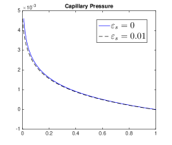
(a) Capillary pressure with epsilon

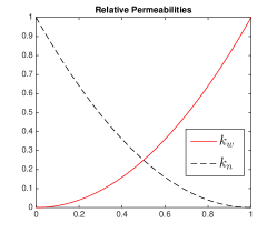
(b) Relative permeabilities

Figure 4: Example 1. Given capillary pressure (64) values and relative permeabilities (65).

The capillary pressure is defined as

$$p_{c}(s_{w}):=\dfrac{B_{c}}{\sqrt{K}}\log({s}_{w}+\varepsilon_{s}),$$ (64)

where $K$ is the absolute permeability in Darcy scale (i.e $$1\text{\,}\mathrm{D}$=$9.869\,233\text{\times}{10}^{-13}\text{\,}\mathrm{m}^{2}$)$ and $K=K_{D}I$ with $K_{D}=${10}^{-5}\text{\,}\mathrm{D}$$, where $I$ is an identity matrix, $B_{c}=-{0.0001}$ and $\varepsilon_{s}=0.01$ to avoid zero singularity (see Figure 4a ). If $s_{w}+\varepsilon_{s}\geq 1$ then we set to $s_{w}+\varepsilon_{s}=1$. Relative permeabilities are given as a function of the wetting phase saturation,

$$k_{w}(s_{w}):=s_{w}^{2},\ \text{ and }\ k_{n}(s_{w}):=(1-s_{w})^{2};$$ (65)

see Figure 4b for more details. In addition, we define following the parameters: $\mu_{w}=$1\text{\,}\mathrm{c}\mathrm{p}$$, $\mu_{n}=$2\text{\,}\mathrm{c}\mathrm{p}$$, $\rho_{w}=\rho_{n}=$1000\text{\,}\mathrm{k}\mathrm{g}\mathrm{/}\mathrm{m}^{3}$$, ${\bf g}=[0,$-9.8\text{\,}\mathrm{m}\mathrm{/}\mathrm{s}^{2}$]/101325$ (scaling with pressure (atm) $$1\text{\,}\mathrm{a}\mathrm{t}\mathrm{m}$=$101\,325\text{\,}\mathrm{Pa}$$), $c_{w}^{F}=${10}^{-12}$$, and $\phi=0.8$.

We illustrate the convergence of EG flow (36) and EG saturation (43), separately for the two-phase flow system with capillary pressure. In this case, exact values of $s_{w}(t^{k})$ and $s_{w}(t^{k-1})$ are provided to compute $P_{w}^{k+1}$, and exact values of $p_{w}(t^{k})$ and $p_{w}(t^{k-1})$ are provided to compute each $S_{w}^{k+1}$. The entropy residual stabilization term (49) discussed in Section 3.3.1 is included with $\lambda_{\textsf{Ent}}=\lambda_{\textsf{Lin}}=${10}^{-2}$$ and entropy function (57) chosen with $\varepsilon=${10}^{-4}$$. The penalty coefficients are set as $\alpha=100$ and $\alpha_{T}=0.01$. For each of the flow and transport equations, respectively, five computations on uniform meshes were computed where the mesh size $h$ is divided by two for each cycle. The time discretization is chosen fine enough not to influence the spatial errors and the time step $\Delta t$ is divided by two for each cycle. Each cycle has $100,200,400,800$ and $1600$ time steps and the errors are computed at the final time $\mathbb{T}=0.1$.

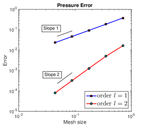
(a) Pressure Error

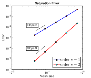
(b) Saturation Error

Figure 5: Example 1. Decoupled case. Error convergence rates for pressure and saturation in semi-$H^{1}$ norm and $L^{2}$ norm, respectively. Optimal order of convergences are observed for both linear and quadratic order cases.

The behavior of the $H^{1}(\Omega)$ semi norm errors for the approximated pressure solution versus the mesh size $h$ are depicted in Figure 5a. Next, the $L^{2}(\Omega)$ error for the approximated saturation solutions versus the mesh size is illustrated in Figure 5b. Both linear and quadratic orders ($l,s=1,2$) were tested and the optimal order of convergences as discussed in [51] are observed.

4.2 Example 2. Convergence Tests - coupled case

In this section, we solve the same problem as in the previous example but with a pressure and saturation system coupled. Here, two different algorithms were tested and compared: sequential IMPES (Section 3.1.1) and iterative IMPES (Section 3.1.2). The convergences of the errors for the pressure and the saturation are provided in Figures 6 and 7. We observed that the optimal rates of convergence for the high order cases ($l=2,s=2$) are obtained for both the sequential and iterative IMPES scheme. Here the tolerance was set to $\varepsilon_{I}=${10}^{-10}$$ and 3-4 iterations were required for the convergence at each time step for iterative IMPES.

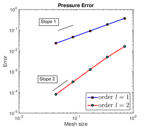
(a) Pressure Error

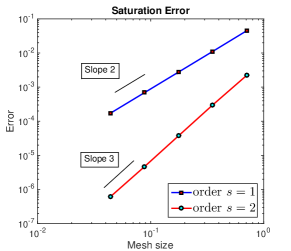
(b) Saturation Error

Figure 6: Example 2. Coupled case (sequential IMPES). Error convergence rates for pressure and saturation in semi-$H^{1}$ norm and $L^{2}$ norm, respectively.

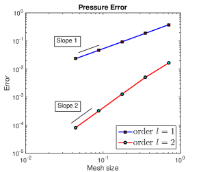
(a) Pressure Error

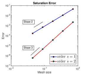
(b) Saturation Error

Figure 7: Example 2. Coupled case (iterative IMPES). Error convergence rates for pressure and saturation in $H^{1}$ semi norm and $L^{2}$ norm, respectively.

4.3 Example 3. A homogeneous channel.

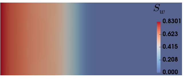
(a) $s_{w}$ value.

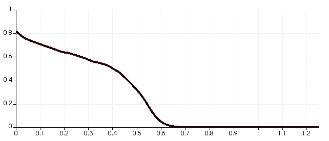
(b) $S_{w}$ value over line $y=0.25$.

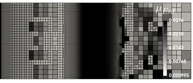
(c) $\mu_{{\textsf{Ent}}}(S_{w},\hat{{\bf U}}_{w})_{|T}$ values.

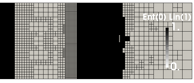
(d) Choices of the stabilization coefficient.

Figure 8: Example 3. Numerical results at time step number $k=50$. (a) wetting phase saturation value. (b) values at (a) are plotted over the fixed line $y=0.25$. (c) entropy residual viscosity values for each cell. (d) choices of viscosities; linear viscosity is chosen where the entropy residual values are larger.

In this example, we illustrate the computational features of our algorithms including entropy viscosity stabilization and dynamic mesh adaptivity with zero capillary pressure. The computational domain is $\Omega=({0},$0\text{\,}\mathrm{m}$)\times($1.25\text{\,}\mathrm{m}$,$0.5\text{\,}\mathrm{m}$)$ and the domain is saturated with a non-wetting phase, residing fluid ($s^{0}_{n}=1$ and $s^{0}_{w}=0$). A wetting phase fluid is injected at the left-hand side of the domain, thus

$$p_{w,\textsf{in}}=$1\text{\,}\mathrm{a}\mathrm{t}\mathrm{m}$,\ s_{w,\textsf{in}}=1\ \text{ on }\ x=$0\text{\,}\mathrm{m}$.$$

On the right hand side, we impose

$$p_{w,\textsf{out}}=$0\text{\,}\mathrm{a}\mathrm{t}\mathrm{m}$\ \text{ on }\ x=$1.25\text{\,}\mathrm{m}$,$$

and no-flow boundary conditions on the top and the bottom of the domain. Fluid and rock properties are given as $\mu_{w}=$1\text{\,}\mathrm{c}\mathrm{P}$$, $\mu_{n}=$3\text{\,}\mathrm{c}\mathrm{P}$$, $\rho_{w}=$1000\text{\,}\mathrm{k}\mathrm{g}\mathrm{/}\mathrm{m}^{3}$$, $\rho_{n}=$830\text{\,}\mathrm{k}\mathrm{g}\mathrm{/}\mathrm{m}^{3}$$, $K_{D}=$1\text{\,}\mathrm{D}$$, $c_{w}^{F}=${10}^{-8}$$ and $\phi=0.2$. Relative permeabilities are given as a function of the wetting phase saturation (65), and the capillary pressure is set to zero for this case. The penalty coefficients are set as $\alpha=100$ and $\alpha_{T}=100$.

Figure 8 illustrates the wetting phase saturation ($s_{w}$) at the time step number $k=50$ with the entropy stabilization coefficients ($\lambda_{\textsf{Ent}}=0.1$, $\lambda_{\textsf{Lin}}=1$) and entropy function (57) chosen with $\varepsilon=${10}^{-4}$$. Dynamic mesh adaptivity is employed with initial refinement level $\textsf{Ref}_{T}=4$, maximum refinement level $R_{\max}=6$ and minimum refinement level $R_{\min}=2$. Here $C_{R}$ is chosen to mark and refine the cells which represent the top 20$\%$ of the values (59) over the domain and $C_{C}$ is chosen to mark and coarsen the cells which represent the bottom 5$\%$ of the values (59) over the domain. The initial number of cells was approximately $2000$ and maximum cell number was approximately $6000$ with a minimum mesh size $h_{\min}=$1.1\text{\times}{10}^{-02}$$. The uniform time step size was chosen as $\Delta t=$5\text{\times}{10}^{-3}$$ (CFL constant around $0.5$). Figure 8b plots the values of $S_{w}$ over the fixed line $y=$0.25\text{\,}\mathrm{m}$$. We observe a saturation front without any spurious oscillations. In addition, Figure 8c presents the adaptive mesh refinements and entropy residual values (58) at the time step number $k=50$. This choice of stabilization (51) performs as expected; see Figure 8d. We note that the linear viscosity (52) is chosen where the entropy residual values are larger.

4.4 Example 4. A layered three dimensional domain

This example presents a three dimensional computation in $\Omega=(0,$1\text{\,}\mathrm{m}$)^{3}$ with a given heterogeneous domain, see Figure 9 for details and boundary conditions. Permeabilities are defined as $K_{D}=\max(\exp(-d_{1}^{2}/0.01),0.01)$, where $d_{1}=|y-0.75-0.1*\sin(10x)|$ for $y>0.5$ and $K_{D}=\max(\exp(-d_{2}^{2}/0.01),0.01)$, where $d_{2}=|y-0.25-0.2*\sin(x)|$ for $y<0.5$. All other physical parameters are the same as in the previous example.

Figure 9: Example 4. Setup with a given permeability ($K_{D}$ values).

Figure 10 illustrates the wetting phase saturation ($S_{w}$) at the time step number $k=10,50,200,$ and $300$ with the entropy stabilization coefficients ($\lambda_{\textsf{Ent}}=0.25$, $\lambda_{\textsf{Lin}}=0.5$) and entropy function (57) chosen with $\varepsilon=${10}^{-3}$$. Dynamic mesh adaptivity is employed with $\textsf{Ref}_{T}=4$, $R_{\max}=6$ and $R_{\min}=2$. The number of cells at $k=300$ is around $262\,100$ and the minimum mesh size is $h_{\min}=$0.027$$ with a time step size $\Delta t=0.006$ (CFL constant is 1). See figures 10b-10d for adaptive mesh refinements for different time steps. The adaptive mesh refinement strategy becomes very efficient for large-scale three dimensional problems using parallelization.

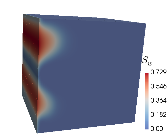
(a) $k=10$

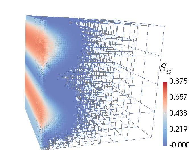
(b) $k=10$ with mesh

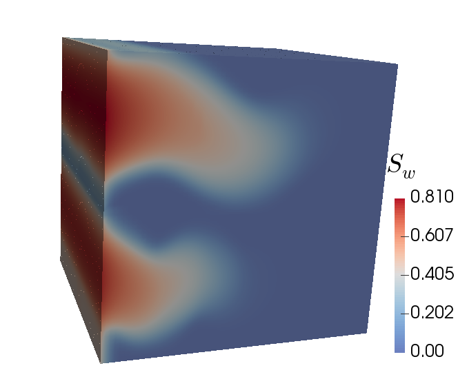
(c) $k=50$

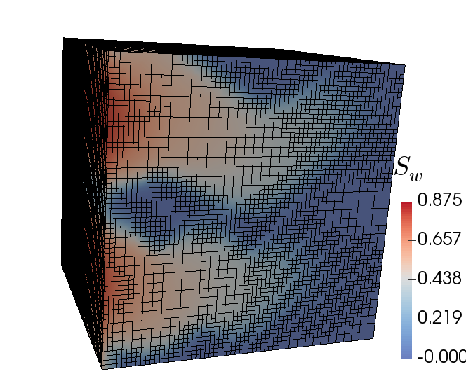
(d) $k=100$ with mesh

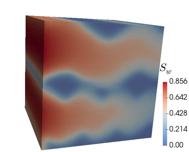
(e) $k=200$

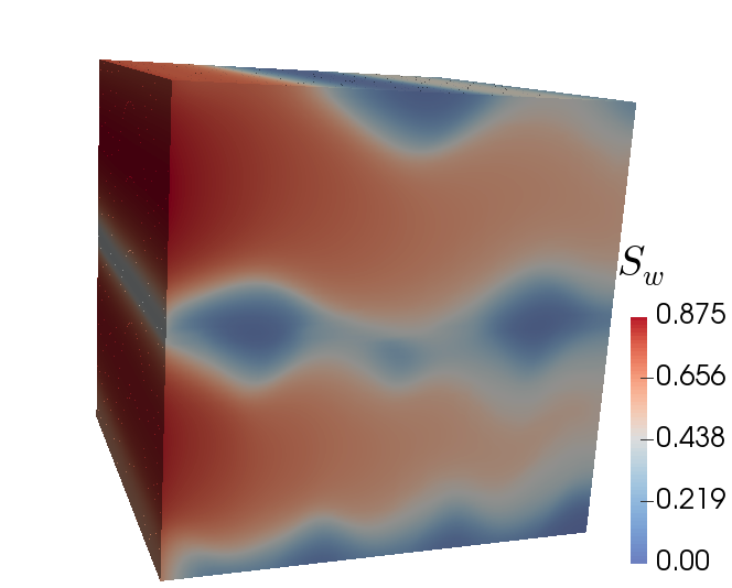
(f) $k=300$

Figure 10: Example 4. The wetting phase saturation ($S_{w}$) at each time step number with adaptive mesh refinements.

4.5 Example 5. A benchmark: effects of capillary pressure

In this example, we emphasize the effects of capillary pressure in a heterogeneous media as shown in [41, 74]. Here, we impose layers of different permeabilities in the computational domain $\Omega=($0\text{\,}\mathrm{m}$,$0\text{\,}\mathrm{m}$)\times($1.25\text{\,}\mathrm{m}$,$0.875\text{\,}\mathrm{m}$)$. See Figure 11.

Figure 11: Example 5. Two dimensional domain with heterogeneous permeabilities. Layered setup to test the effect of the capillary pressure. Permeabilities are defined as $K_{D}=$0.01\text{\,}\mathrm{D}$$ for the dark region and $K_{D}=$1\text{\,}\mathrm{D}$$ for the white region.

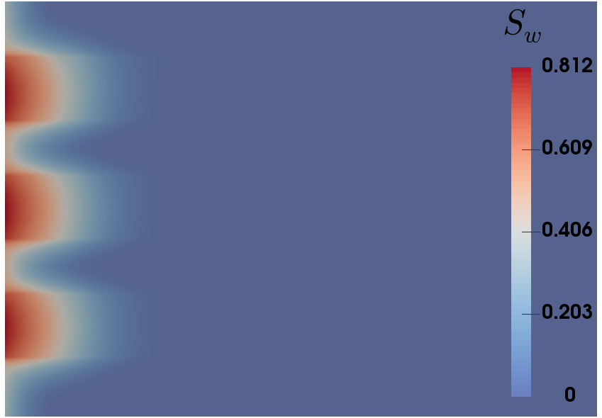
(a) $k=125$

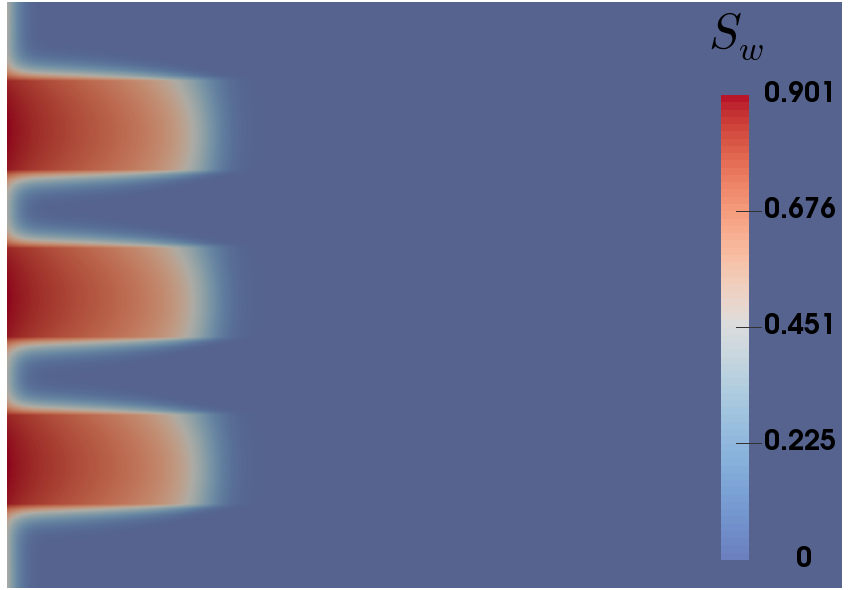
(b) $k=125$

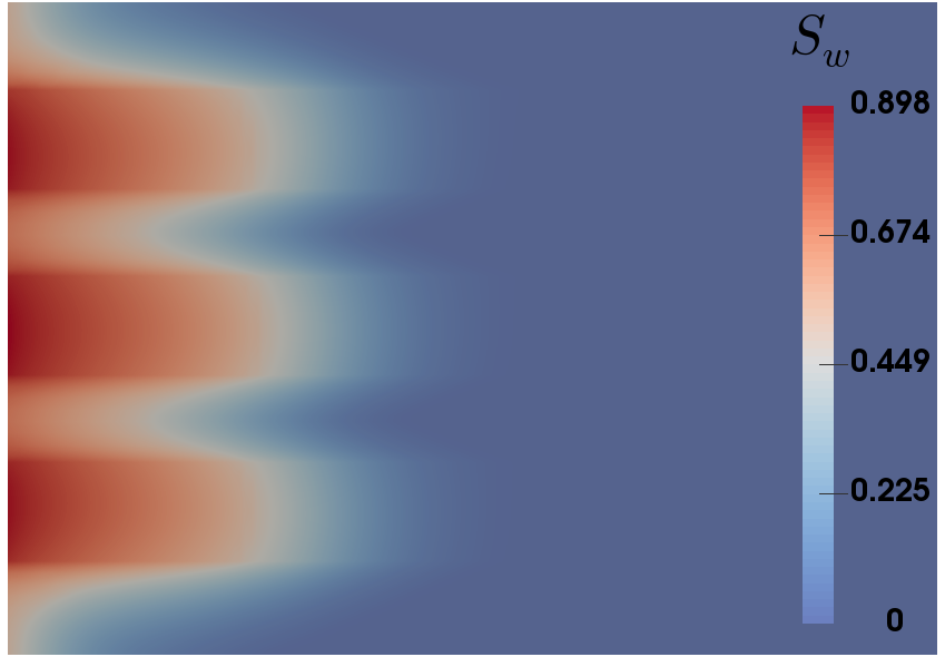
(c) $k=375$

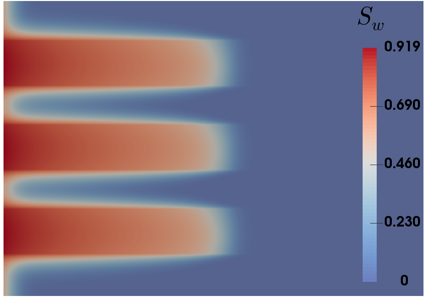
(d) $k=375$

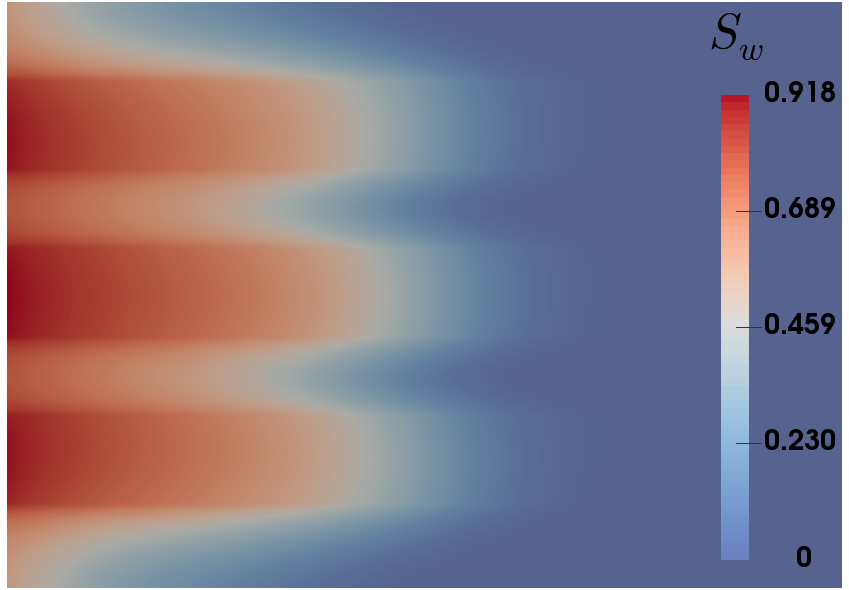
(e) $k=625$

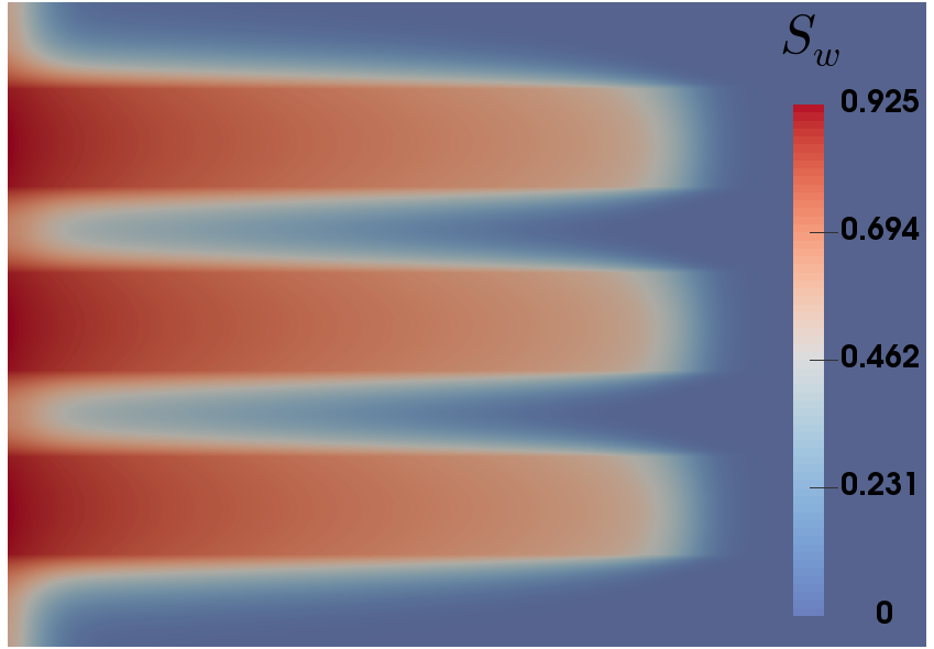
(f) $k=625$

Figure 12: Example 5. Wetting phase saturation values at each time step number. The left column (a),(c), and (e) are the values with the capillary pressure and the right column (b),(d), and (f) are the values without the capillary pressure.

The domain is saturated with a non-wetting phase (oil), i.e $s^{0}_{n}=1$ and $s^{0}_{w}=0$. A wetting phase fluid is injected at the left-hand side of the domain, thus

$$p_{w,\textsf{in}}=$0.1\text{\,}\mathrm{a}\mathrm{t}\mathrm{m}$,\ s_{w,\textsf{in}}=1\ \text{ on }\ x=$0\text{\,}\mathrm{m}$.$$

On the right hand side, we impose

$$p_{w,\textsf{out}}=$0\text{\,}\mathrm{a}\mathrm{t}\mathrm{m}$\ \text{ on }\ x=$1.25\text{\,}\mathrm{m}$,$$

and no-flow boundary conditions on the top and the bottom of the domain. Fluid properties are set as $\mu_{w}=$1\text{\,}\mathrm{c}\mathrm{P}$$, $\mu_{n}=$0.45\text{\,}\mathrm{c}\mathrm{P}$$, $\rho_{w}=$1000\text{\,}\mathrm{k}\mathrm{g}\mathrm{/}\mathrm{m}^{3}$$, $\rho_{n}=$660\text{\,}\mathrm{k}\mathrm{g}\mathrm{/}\mathrm{m}^{3}$$, $c_{w}^{F}=${10}^{-8}$$, $\phi=0.2$, and $K_{D}=$1\text{\,}\mathrm{D}$$ or $K_{D}=$0.01\text{\,}\mathrm{D}$$ as illustrated in Figure 11. Relative permeabilities are given as a function of the wetting phase saturation (65), and the penalty coefficients are set as $\alpha=1$, $\alpha_{c}=1$ and $\alpha_{T}=1000$. The entropy stabilization coefficients are $\lambda_{\textsf{Ent}}=1$ and $\lambda_{\textsf{Lin}}=1$. Dynamic mesh adaptivity is employed as same as the example 3 and the minimum mesh size is $h_{\min}=$0.0027$$. The uniform time step size is taken as $\Delta t=$0.005$$. The capillary pressure (64) is given with $B_{c}=-0.01$ and $\varepsilon_{s}=0.1$.

Here two tests are performed, one with the capillary pressure ($B_{c}=-0.01$) and a second with zero capillary pressure ($B_{c}=0$). The differences and effects of capillary pressure are depicted at Figure 12 for different time steps. The injected wetting phase water flows faster in the high permeability layers but is more diffused in the case with capillary pressure as shown in previous results [41, 74]. One can observe the capillary pressure is a non-linear diffusion source term for the residing non-wetting phase. This causes more uniformed movement of the injected fluid.

4.6 Example 6. A random heterogeneous domain with different relative permeability

This example considers well injection and production in a random heterogeneous domain $\Omega=($0\text{\,}\mathrm{,}$$1\text{\,}\mathrm{m}$)^{2}$. Wells are specified at the corners with injection at $(0,0)$ and production at $($1\text{\,}\mathrm{m}$,$1\text{\,}\mathrm{m}$)$. See Figure 13a for the setup. We test and compare two different non-wetting phase relative permeabilities such as

$$\text{i) }k^{1}_{n}(s_{w}):={(1-s_{w})^{2}}\ \text{ and }\ \text{ii) }k^{2}_{n}(s_{w}):=\dfrac{(1-s_{w})^{2}}{f_{w}},$$ (66)

where the latter is often referred as the case with foam in a porous media [59]. Here, $f_{w}:=1+R(0.5+\dfrac{1}{\pi}\arctan(\kappa(s_{w}-s_{w}^{*})))$ is a mobility reduction factor with a constant positive parameters set to $R=10$, $\kappa=100$, and a limiting water saturation $S_{w}^{*}=0.3$. Figure 13b illustrates two different non-wetting phase relative permeabilities ($k^{1}_{n},k^{2}_{n}$). The wetting phase relative permeability ($k_{w}$) is identical with the previous examples.

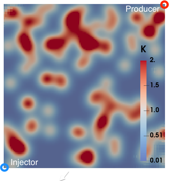
(a) Permeability $K$ values

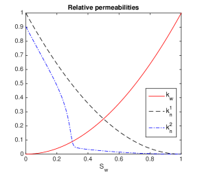
(b) Relative permeabilities

Figure 13: Example 6. Setup with a random absolute permeabilities, wetting phase relative permeability $(k_{w})$, and two different non-wetting phase relative permeabilities ($k^{1}_{n},k^{2}_{n}$). We note $k^{2}_{n}$ represents rough relative permeability which often referred as the case with foam in a porous media [59].

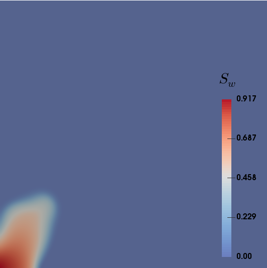
(a) $t=0.76s$

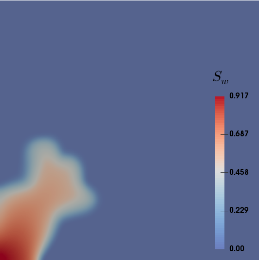
(b) $t=1.9s$

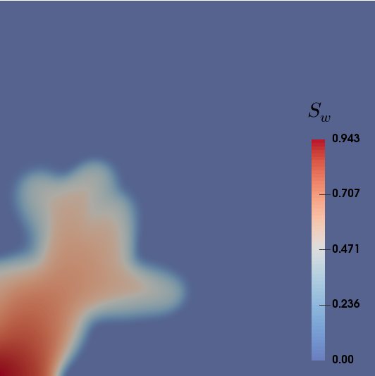
(c) $t=3.04s$

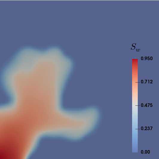
(d) $t=5s$

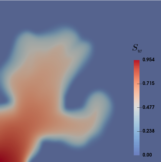
(e) $t=6.84s$

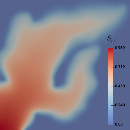
(f) $t=10.64s$

Figure 14: Example 6. $S_{w}$ values for each time in a heterogeneous media with a non-wetting phase relative permeability $k^{1}_{n}(s_{w})$.

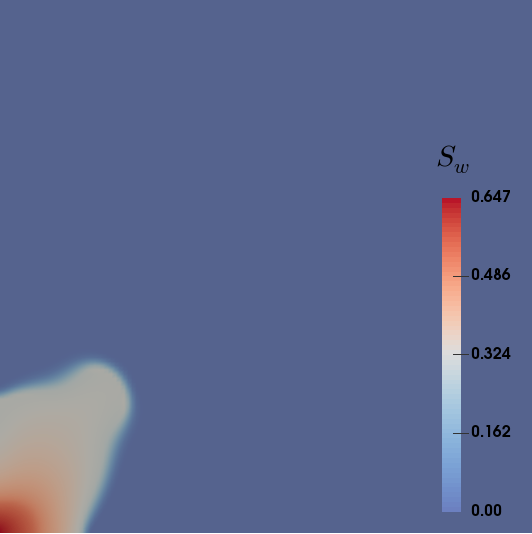
(a) $t=0.765$

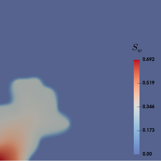
(b) $t=2s$

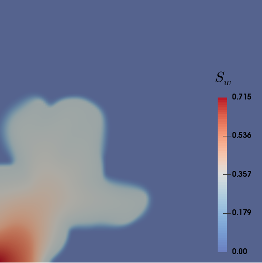
(c) $t=3s$

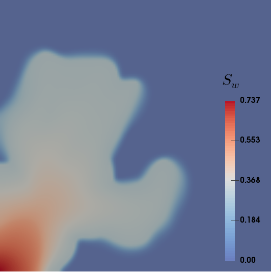
(d) $t=5s$

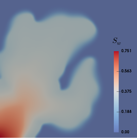
(e) $t=6.8s$

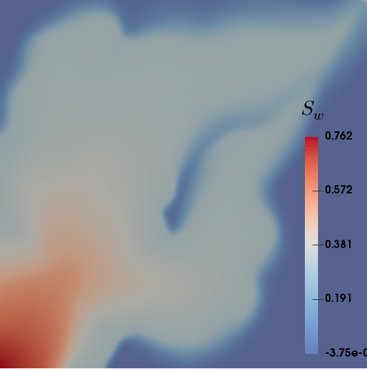
(f) $t=10s$

Figure 15: Example 6. $S_{w}$ values for each time in a heterogeneous media with a non-wetting phase relative permeability $k^{2}_{n}(s_{w})$.

We assume the domain is saturated with a non-wetting phase, i.e $s^{0}_{n}=1$ and $s^{0}_{w}=0$ and a wetting phase fluid is injected. Fluid and rock properties are given as $\mu_{w}=$1\text{\,}\mathrm{c}\mathrm{P}$$, $\mu_{n}=$3\text{\,}\mathrm{c}\mathrm{P}$$, $\rho_{w}=$1000\text{\,}\mathrm{k}\mathrm{g}\mathrm{/}\mathrm{m}^{3}$$, $\rho_{n}=$830\text{\,}\mathrm{k}\mathrm{g}\mathrm{/}\mathrm{m}^{3}$$, $c_{w}^{F}=${10}^{-10}$$, $f_{w}^{+}=$100\text{\,}\mathrm{m}\mathrm{/}\mathrm{s}$$, $f_{w}^{-}=-$100\text{\,}\mathrm{m}\mathrm{/}\mathrm{s}$$, $f_{n}=0$, and $\phi=0.2$. The capillary pressure and the gravity is neglected to emphasize the effects of heterogeneity and different non-wetting phase relative permeability. Here the numerical parameters are chosen as $h_{\min}=$1.1\text{\times}{10}^{-02}$$ and $\Delta t=$3.8\text{\times}{10}^{-03}$$. Due to the dynamic mesh refinement ($\textsf{R}_{\max}=7$ and $\textsf{R}_{\min}=2$), the number of degrees of freedom for EG transport and the maximum number of cells are $32158$, $15934$, respectively at the final time $\mathbb{T}=15$. The entropy stabilization coefficients are set to $\lambda_{\textsf{Ent}}=0.1$ and $\lambda_{\textsf{Lin}}=0.25$, where the entropy function (57) is chosen with $\varepsilon=${10}^{-3}$$. The penalty coefficients are set as $\alpha=1$ and $\alpha_{T}=1000$.

Figure 14 illustrates the EG-${\mathbb{Q}}_{1}$ solution of $S_{w}$ values for each time in a heterogeneous media with a non-wetting phase relative permeability $k^{1}_{n}(s_{w})$. Next, Figure 15 is the case with $k^{2}_{n}(s_{w})$. We note that wetting phase saturation values above $S_{w}^{*}$ are restricted for the latter case due to the relative permeability, $k^{2}_{n}(s_{w})$.

4.7 Example 7. A three dimensional random heterogeneous domain

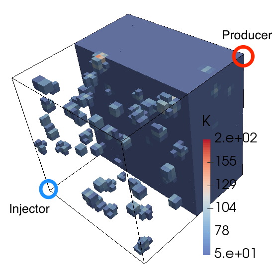
Figure 16: Example 7. Setup with a random absolute permeabilities in a three dimensional domain.

In this example, we simply extend the previous example to a three dimensional domain $\Omega=($0\text{\,}\mathrm{,}$$1\text{\,}\mathrm{m}$)^{3}$ with absolute permeabilities given as figure 16. Wells are specified at the corners with injection at $(0,0,0)$ and production at $($1\text{\,}\mathrm{m}$,$1\text{\,}\mathrm{m}$,$1\text{\,}\mathrm{m}$)$. The numerical parameters are chosen as $h_{\min}=$5.4\text{\times}{10}^{-02}$$ and $\Delta t=$3.4\text{\times}{10}^{-03}$$. All the other physical parameters and boundary conditions are the same as in the previous example.

Figure 17 illustrates the contour value of $S_{w}=0.3$ for each time step. Here the maximum EG-${\mathbb{Q}}_{1}$ degrees of freedom for wetting phase saturation at the final time step is around $70,000$ and this example is computed by employing four multiple parallel processors (MPI).

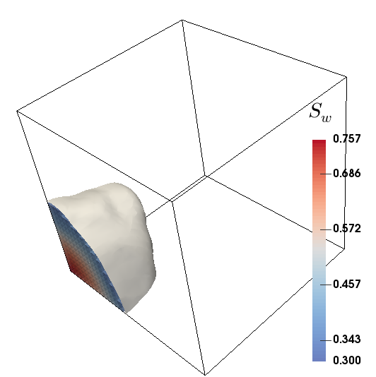
(a) $k=110$

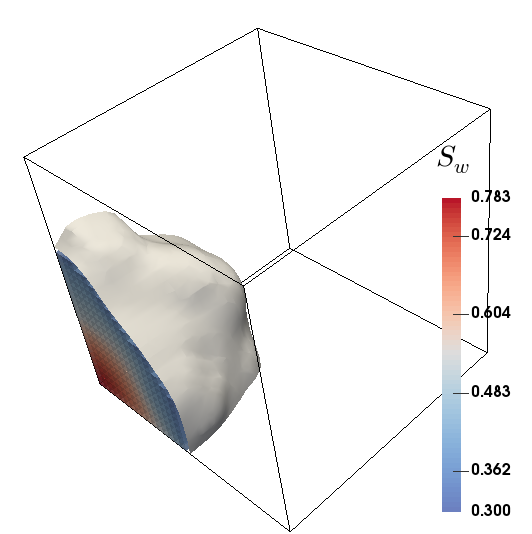
(b) $k=210$

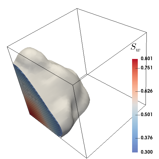
(c) $k=360$

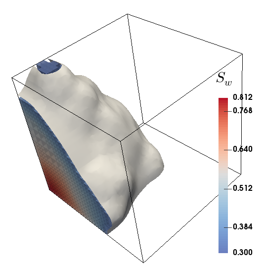
(d) $k=510$

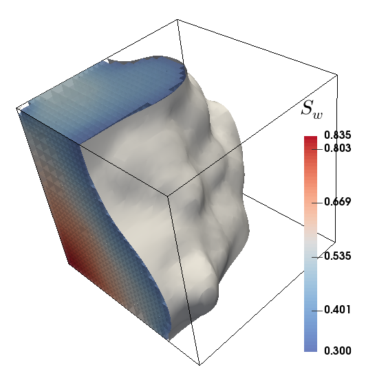
(e) $k=1010$

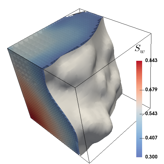
(f) $k=1290$

Figure 17: Example 7. Contour value $S_{w}=0.3$ for each time step.

4.8 Example 8. Well injections with gravity and a capillary pressure

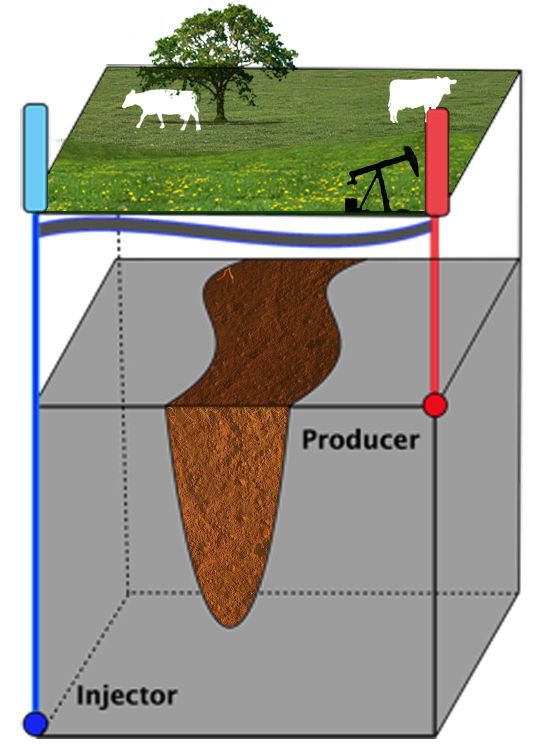
(a) Setup

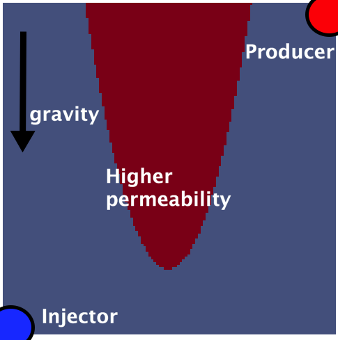
(b) A domain

Figure 18: Example 6. Setup with the domain and the boundary conditions. (b) Two dimensional computational domain is defined by slicing the three dimensional domain (a) vertically. Bottom blue is the injection well and top red is the production well in the reservoir. Higher permeability zone is in the middle due to long sediments.

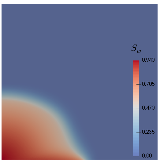
(a) t=145s

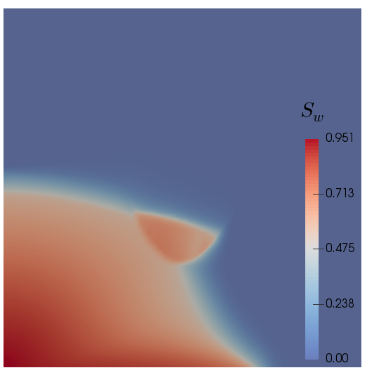
(b) t=250s

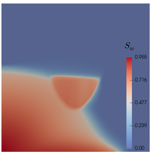
(c) t=325s

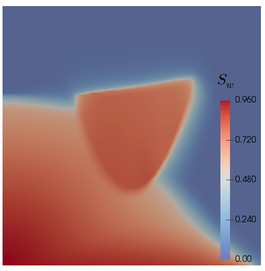
(d) t=500s

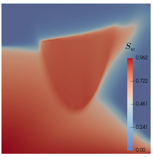
(e) t=685s

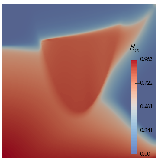
(f) t=720s

Figure 19: Example 6. The wetting phase saturation ($S_{w}$) at each time.

Figure 18a illustrates an example of an existing reservoir where we have sliced a computational domain vertically, $\Omega=($0\text{\,}\mathrm{m}$,$50\text{\,}\mathrm{m}$)^{2}$ as shown in Figure 18b. Wells are rate specified at the corners with injection at $(0,0)$ and production at $($50\text{\,}\mathrm{m}$,$50\text{\,}\mathrm{m}$)$. A high permeability zone representing long sediments is located at ($y\geq 0.16x^{2}-7.78x+112.22$), where $K_{D}=$10\text{\,}\mathrm{D}$$ and $K_{D}=$1\text{\,}\mathrm{D}$$ otherwise. We assume the domain is saturated with a non-wetting phase, i.e $s^{0}_{n}=1$ and $s^{0}_{w}=0$ and a wetting phase fluid is injected. Fluid and rock properties are given as $\mu_{w}=$1\text{\,}\mathrm{c}\mathrm{P}$$, $\mu_{n}=$3\text{\,}\mathrm{c}\mathrm{P}$$, $\rho_{w}=$1000\text{\,}\mathrm{k}\mathrm{g}\mathrm{/}\mathrm{m}^{3}$$, $\rho_{n}=$830\text{\,}\mathrm{k}\mathrm{g}\mathrm{/}\mathrm{m}^{3}$$, $c_{w}^{F}=${10}^{-10}$$, $f_{w}^{+}=$2.5\text{\,}\mathrm{m}\mathrm{/}\mathrm{s}$$, $f_{w}^{-}=-$2.5\text{\,}\mathrm{m}\mathrm{/}\mathrm{s}$$, $f_{n}=0$, and $\phi=0.2$. Relative permeabilities are given as functions of the wetting phase saturation (65), and the capillary pressure is set with $B_{c}=-0.001$ and $\varepsilon_{s}=0.1$. The penalty coefficients are set as $\alpha=1$, $\alpha_{c}=1$ and $\alpha_{T}=1000$ and the time step is set by $\Delta t=$0.18$$. Here, we employ the gravity ${\bf g}=[0,$-9.8\text{\,}\mathrm{m}\mathrm{/}\mathrm{s}^{2}$$], and for the same scaling with pressure (atm), we divide it by ${101325}$ ($$1\text{\,}\mathrm{a}\mathrm{t}\mathrm{m}$=$101\,325\text{\,}\mathrm{Pa}$$). Figure 19 illustrates the injected wetting phase saturation values for each time step number. We observe the effect of the gravity.

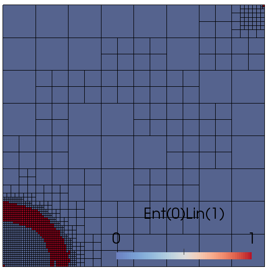
(a) $t=$14.5\text{\,}\mathrm{s}$$

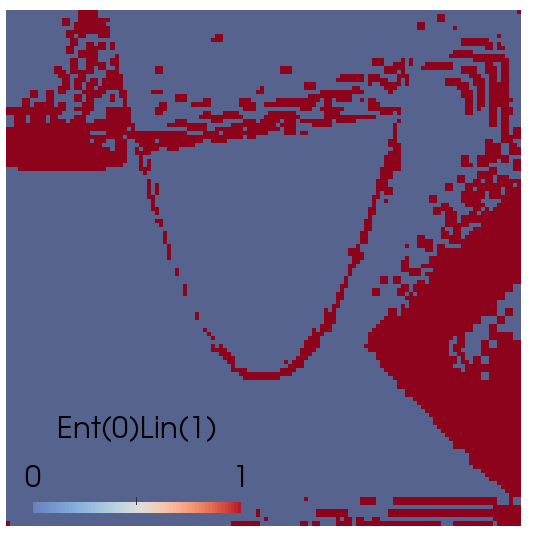
(b) $t=$650\text{\,}\mathrm{s}$$

Figure 20: Example 6. Entropy choices for early and later time.

The entropy stabilization coefficients are set as $\lambda_{\textsf{Ent}}=40$ and $\lambda_{\textsf{Lin}}=1$, where the entropy function (57) is chosen with $\varepsilon=${10}^{-3}$$. Figure 20 illustrates the choice for stabilization. Dynamic mesh adaptivity is employed with initial refinement level $\textsf{Ref}_{T}=4$, $R_{\max}=7$ and $R_{\min}=3$ with a minimum mesh size is $h_{\min}=$0.4$$. In addition, Figure 21 presents the production data. The oil saturation values (non-wetting phase $S_{n}$) over the time are plotted with the accumulative oil production rate ($\sum_{k=0}^{\mathbb{T}}|S_{n}{f}^{-}|$).

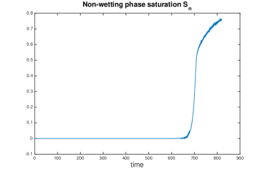
(a) $S_{n}$ values in time

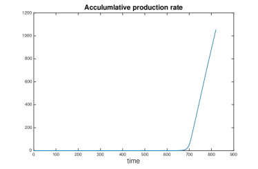
(b) Accumulative oil production rate ($\sum f\times S_{n}$)

Figure 21: Example 6. Production data

5 Conclusion

In this paper, we present enriched Galerkin (EG) approximations for two-phase flow problems in porous media with capillary pressure. EG preserves local and global conservation for fluxes and has fewer degrees of freedom compared to DG. For a high order EG transport system, entropy residual stabilization is applied to avoid spurious oscillations. In addition, dynamic mesh adaptivity employing entropy residual as an error indicator reduces computational costs for large-scale computations. Several examples in two and three dimensions including error convergences and a well known capillary pressure benchmark problem are shown in order to verify and demonstrate the performance of the algorithm. Additional challenging effects arising from gravity and rough relative permeabilities for foam are presented.

References

- [1] Andrews, J., Morton, K.: A posteriori error estimation based on discrepancies in an entropy variable. International Journal of Computational Fluid Dynamics 10(3), 183–198 (1998)
- [2] Arbogast, T.: The existence of weak solutions to single porosity and simple dual-porosity models of two-phase incompressible flow. Nonlinear Analysis: Theory, Methods & Applications 19(11), 1009–1031 (1992)
- [3] Arbogast, T.: Numerical subgrid upscaling of two-phase flow in porous media. In: Numerical treatment of multiphase flows in porous media, pp. 35–49. Springer (2000)
- [4] Arbogast, T.: Implementation of a locally conservative numerical subgrid upscaling scheme for two-phase darcy flow. Computational Geosciences 6(3-4), 453–481 (2002)
- [5] Arbogast, T., Juntunen, M., Pool, J., Wheeler, M.F.: A discontinuous Galerkin method for two-phase flow in a porous medium enforcing H (div) velocity and continuous capillary pressure. Computational Geosciences 17(6), 1055–1078 (2013)
- [6] Arbogast, T., Wheeler, M.F., Yotov, I.: Mixed finite elements for elliptic problems with tensor coefficients as cell-centered finite differences. SIAM Journal on Numerical Analysis 34(2), 828–852 (1997)
- [7] Aziz, K., Settari, A.: Petroleum reservoir simulation. Chapman & Hall (1979)
- [8] Bangerth, W., Davydov, D., Heister, T., Heltai, L., Kanschat, G., Kronbichler, M., Maier, M., Turcksin, B., Wells, D.: The deal.II library, version 8.4. Journal of Numerical Mathematics 24(3), 135–141 (2016). DOI 10.1515/jnma-2016-1045
- [9] Bastian, P.: A fully-coupled discontinuous galerkin method for two-phase flow in porous media with discontinuous capillary pressure. Computational Geosciences 18(5), 779–796 (2014)
- [10] Bastian, P., Rivière, B.: Superconvergence and H-(div) projection for discontinuous galerkin methods. International journal for numerical methods in fluids 42(10), 1043–1057 (2003)
- [11] Becker, R., Burman, E., Hansbo, P., Larson, M.G.: A reduced P1-discontinuous Galerkin method. Chalmers Finite Element Center Preprint 2003-13 (2003)
- [12] Boffi, D., Brezzi, F., Fortin, M., et al.: Mixed finite element methods and applications, vol. 44. Springer (2013)
- [13] Bonito, A., Guermond, J.L., Lee, S.: Numerical simulations of bouncing jets. International Journal for Numerical Methods in Fluids 80(1), 53–75 (2016). DOI 10.1002/fld.4071. Fld.4071
- [14] Bonito, A., Guermond, J.L., Popov, B.: Stability analysis of explicit entropy viscosity methods for non-linear scalar conservation equations. Math. Comp. 83(287), 1039–1062 (2014)
- [15] Burstedde, C., Wilcox, L.C., Ghattas, O.: p4est: Scalable algorithms for parallel adaptive mesh refinement on forests of octrees. SIAM Journal on Scientific Computing 33(3), 1103–1133 (2011)
- [16] Chavent, G., Jaffré, J.: Mathematical models and finite elements for reservoir simulation: single phase, multiphase and multicomponent flows through porous media, vol. 17. Elsevier (1986)
- [17] Chen, Z., Huan, G., Li, B.: An improved impes method for two-phase flow in porous media. Transport in Porous Media 54(3), 361–376 (2004)
- [18] Chen, Z., Huan, G., Ma, Y.: Computational Methods for Multiphase Flows in Porous Media. Society for Industrial and Applied Mathematics (2006)
- [19] Coats, K., et al.: Reservoir simulation: State of the art (includes associated papers 11927 and 12290). Journal of Petroleum Technology 34(08), 1–633 (1982)
- [20] Coats, K.H., et al.: A note on IMPES and some IMPES-based simulation models. SPE Journal 5(03), 245–251 (2000)
- [21] Dawson, C., Sun, S., Wheeler, M.F.: Compatible algorithms for coupled flow and transport. Comput. Methods Appl. Mech. Engrg. 193(23-26), 2565–2580 (2004)
- [22] Douglas, J.J., Darlow, B.L., Wheeler, M., Kendall, R.P.: Self-Adaptive Galerkin Methods For One-Dimensional, Two-Phase Immiscible Flow. Society of Petroleum Engineers (1979)
- [23] Efendiev, Y., Ginting, V., Hou, T., Ewing, R.: Accurate multiscale finite element methods for two-phase flow simulations. Journal of Computational Physics 220(1), 155–174 (2006)
- [24] Efendiev, Y.R., Durlofsky, L.J., et al.: Accurate subgrid models for two-phase flow in heterogeneous reservoirs. In: SPE Reservoir Simulation Symposium. Society of Petroleum Engineers (2003)
- [25] El-Amin, M.F., Kou, J., Sun, S., Salama, A.: An iterative implicit scheme for nanoparticles transport with two-phase flow in porous media. Procedia Computer Science 80, 1344 – 1353 (2016)
- [26] Epshteyn, Y., Riviere, B.: Fully implicit discontinuous finite element methods for two-phase flow. Applied Numerical Mathematics 57, 383–401 (2007)
- [27] Epshteyn, Y., Riviere, B.: Analysis of hp discontinuous Galerkin methods for incompressible two-phase flow. Journal of Computational and Applied Mathematics 225, 487–509 (2009)
- [28] Ern, A., Mozolevski, I., Schuh, L.: Accurate velocity reconstruction for discontinuous Galerkin approximations of two-phase porous media flows. Comptes Rendus Mathematique 347(9), 551–554 (2009)
- [29] Ern, A., Mozolevski, I., Schuh, L.: Discontinuous Galerkin approximation of two-phase flows in heterogeneous porous media with discontinuous capillary pressures. Computer Methods in Applied Mechanics and Engineering 199(23-24), 1491–1501 (2010)
- [30] Ern, A., Nicaise, S., Vohralík, M.: An accurate H (div) flux reconstruction for discontinuous Galerkin approximations of elliptic problems. Comptes Rendus Mathematique 345(12), 709–712 (2007)
- [31] Ewing, R., Russell, T., Wheeler, M.F.: Simulation of miscible displacement using mixed methods and a modified method of characteristics. In: SPE Reservoir Simulation Symposium. Society of Petroleum Engineers (1983)
- [32] Fagin, R., Stewart Jr, C., et al.: A new approach to the two-dimensional multiphase reservoir simulator. Society of Petroleum Engineers Journal 6(02), 175–182 (1966)
- [33] Gabriel, E., Fagg, G.E., Bosilca, G., Angskun, T., Dongarra, J.J., Squyres, J.M., Sahay, V., Kambadur, P., Barrett, B., Lumsdaine, A., Castain, R.H., Daniel, D.J., Graham, R.L., Woodall, T.S.: Open MPI: Goals, concept, and design of a next generation MPI implementation. In: Proceedings, 11th European PVM/MPI Users’ Group Meeting, pp. 97–104. Budapest, Hungary (2004)
- [34] Ganis, B., Kumar, K., Pencheva, G., Wheeler, M.F., Yotov, I.: A global Jacobian method for mortar discretizations of a fully implicit two-phase flow model. Multiscale Modeling & Simulation 12(4), 1401–1423 (2014)
- [35] Guermond, J.L., Larios, A., Thompson, T.: Direct and Large-Eddy Simulation IX, chap. Validation of an Entropy-Viscosity Model for Large Eddy Simulation, pp. 43–48. Springer International Publishing, Cham (2015). DOI 10.1007/978-3-319-14448-1$“˙$6
- [36] Guermond, J.L., de Luna, M.Q., Thompson, T.: An conservative anti-diffusion technique for the level set method. Journal of Computational and Applied Mathematics 321, 448 – 468 (2017)
- [37] Guermond, J.L., Pasquetti, R.: Entropy Viscosity Method for High-Order Approximations of Conservation Laws, pp. 411–418. Springer Berlin Heidelberg, Berlin, Heidelberg (2011)
- [38] Guermond, J.L., Pasquetti, R., Popov, B.: Entropy viscosity method for nonlinear conservation laws. Journal of Computational Physics 230(11), 4248–4267 (2011)
- [39] Hajibeygi, H., Jenny, P.: Multiscale finite-volume method for parabolic problems arising from compressible multiphase flow in porous media. Journal of Computational Physics 228(14), 5129 – 5147 (2009)
- [40] Heroux, M., Bartlett, R., Hoekstra, V.H.R., Hu, J., Kolda, T., Lehoucq, R., Long, K., Pawlowski, R., Phipps, E., Salinger, A., Thornquist, H., Tuminaro, R., Willenbring, J., Williams, A.: An Overview of Trilinos. Tech. Rep. SAND2003-2927, Sandia National Laboratories (2003)
- [41] Hoteit, H., Firoozabadi, A.: Numerical modeling of two-phase flow in heterogeneous permeable media with different capillarity pressures. Advances in Water Resources 31(1), 56–73 (2008)
- [42] Jenny, P., Lee, S., Tchelepi, H.: Multi-scale finite-volume method for elliptic problems in subsurface flow simulation. Journal of Computational Physics 187(1), 47–67 (2003)
- [43] Jenny, P., Lee, S.H., Tchelepi, H.A.: Adaptive multiscale finite-volume method for multiphase flow and transport in porous media. Multiscale Modeling & Simulation 3(1), 50–64 (2005)
- [44] Kaasschieter, E.: Mixed finite elements for accurate particle tracking in saturated groundwater flow. Advances in Water Resources 18(5), 277 – 294 (1995)
- [45] Klieber, W., Riviere, B.: Adaptive simulations of two-phase flow by discontinuous Galerkin methods. Computer Methods in Applied Mechanics and Engineering 196, 404–419 (2006)
- [46] Kou, J., Sun, S.: A new treatment of capillarity to improve the stability of impes two-phase flow formulation. Computers & Fluids 39(10), 1923–1931 (2010)
- [47] Kou, J., Sun, S.: On iterative impes formulation for two phase flow with capillarity in heterogeneous porous media. International Journal of Numerical Analysis and Modeling. Series B 1(1), 20–40 (2010)
- [48] Kou, J., Sun, S.: Convergence of discontinuous Galerkin methods for incompressible two-phase flow in heterogeneous media. SIAM Journal on Numerical Analysis 51(6), 3280–3306 (2013)
- [49] Kruz̆kov, S.N.: First order quasilinear equations in several independent variables. Mathematics of the USSR-Sbornik 10(2), 217 (1970)
- [50] Kueper, B.H., Frind, E.O.: Two-phase flow in heterogeneous porous media: 1. model development. Water Resources Research 27(6), 1049–1057 (1991)
- [51] Lee, S., Lee, Y.J., Wheeler, M.F.: A locally conservative enriched Galerkin approximation and efficient solver for elliptic and parabolic problems. SIAM Journal on Scientific Computing 38(3), A1404–A1429 (2016). DOI 10.1137/15M1041109
- [52] Lee, S., Lee, Y.J., Wheeler, M.F.: Enriched Galerkin approximations for coupled flow and transport system (2017). Submitted
- [53] Lee, S., Mikelić, A., Wheeler, M., Wick, T.: Phase-field modeling of two-phase fluid-filled fractures in a poroelastic medium (2017). Submitted
- [54] Lee, S., Mikelić, A., Wheeler, M.F., Wick, T.: Phase-field modeling of proppant-filled fractures in a poroelastic medium. Computer Methods in Applied Mechanics and Engineering 312, 509 – 541 (2016). DOI http://dx.doi.org/10.1016/j.cma.2016.02.008. Phase Field Approaches to Fracture
- [55] Lee, S., Wheeler, M.F.: Adaptive enriched Galerkin methods for miscible displacement problems with entropy residual stabilization. Journal of Computational Physics 331, 19 – 37 (2017)
- [56] Lee, S., Wolfsteiner, C., Tchelepi, H.: Multiscale finite-volume formulation for multiphase flow in porous media: black oil formulation of compressible, three-phase flow with gravity. Computational Geosciences 12(3), 351–366 (2008)
- [57] Li, J., Rivière, B.: High order discontinuous Galerkin method for simulating miscible flooding in porous media. Computational Geosciences pp. 1–18 (2015)
- [58] Lu, B., Wheeler, M.F.: Iterative coupling reservoir simulation on high performance computers. Petroleum Science 6(1), 43–50 (2009)
- [59] van der Meer, J., Farajzadeh, R., Jansen, J., et al.: Influence of foam on the stability characteristics of immiscible flow in porous media. In: SPE Reservoir Simulation Conference. Society of Petroleum Engineers (2017)
- [60] Morel-Seytoux, H.: Two-phase flows in porous media. Advances in Hydroscience 9, 119–202 (1973)
- [61] Panov, E.Y.: Uniqueness of the solution of the cauchy problem for a first order quasilinear equation with one admissible strictly convex entropy. Mathematical Notes 55(5), 517–525 (1994)
- [62] Peaceman, D.: Fundamentals of Numerical Reservoir Simulation. Developments in Petroleum Science. Elsevier Science (2000). URL https://books.google.com/books?id=-DujQRDF4kwC
- [63] Peszyńska, M., Wheeler, M.F., Yotov, I.: Mortar upscaling for multiphase flow in porous media. Computational Geosciences 6(1), 73–100 (2002)
- [64] Puppo, G.: Numerical entropy production for central schemes. SIAM Journal on Scientific Computing 25(4), 1382–1415 (2004)
- [65] Radu, F.A., Nordbotten, J.M., Pop, I.S., Kumar, K.: A robust linearization scheme for finite volume based discretizations for simulation of two-phase flow in porous media. Journal of Computational and Applied Mathematics 289, 134–141 (2015)
- [66] Raviart, P.A., Thomas, J.M.: A mixed finite element method for 2-nd order elliptic problems, pp. 292–315. Springer Berlin Heidelberg, Berlin, Heidelberg (1977)
- [67] Riaz, A., Tchelepi, H.A.: Linear stability analysis of immiscible two-phase flow in porous media with capillary dispersion and density variation. Physics of Fluids 16(12), 4727–4737 (2004)
- [68] Riaz, A., Tchelepi, H.A.: Numerical simulation of immiscible two-phase flow in porous media. Physics of Fluids 18(1), 014,104 (2006)
- [69] Schmid, K., Geiger, S., Sorbie, K.: Higher order FE-FV method on unstructured grids for transport and two-phase flow with variable viscosity in heterogeneous porous media. Journal of Computational Physics 241, 416 – 444 (2013)
- [70] Scovazzi, G., Wheeler, M.F., Mikelić, A., Lee, S.: Analytical and variational numerical methods for unstable miscible displacement flows in porous media. Journal of Computational Physics 335, 444 – 496 (2017)
- [71] Slattery, J.C.: Two-phase flow through porous media. AIChE Journal 16(3), 345–352 (1970)
- [72] Sun, S., Liu, J.: A Locally Conservative Finite Element Method based on piecewise constant enrichment of the continuous Galerkin method. SIAM J. Sci. Comput. 31, 2528–2548 (2009)
- [73] Whitaker, S.: Flow in porous media ii: The governing equations for immiscible, two-phase flow. Transport in porous media 1(2), 105–125 (1986)
- [74] Yang, H., Sun, S., Yang, C.: Nonlinearly preconditioned semismooth newton methods for variational inequality solution of two-phase flow in porous media. Journal of Computational Physics 332, 1–20 (2017)
- [75] Young, L.C., Stephenson, R.E., et al.: A generalized compositional approach for reservoir simulation. Society of Petroleum Engineers Journal 23(05), 727–742 (1983)
- [76] Zhang, N., Huang, Z., Yao, J.: Locally conservative Galerkin and finite volume methods for two-phase flow in porous media. Journal of Computational Physics 254, 39 – 51 (2013)
- [77] Zingan, V., Guermond, J.L., Morel, J., Popov, B.: Implementation of the entropy viscosity method with the discontinuous Galerkin method. Computer Methods in Applied Mechanics and Engineering 253, 479–490 (2013)