The impact of the injection protocol on an impurity’s stationary state

Abstract

We examine stationary state properties of an impurity particle injected into a one-dimensional quantum gas. We show that the value of the impurity’s end velocity lies between zero and the speed of sound in the gas, and is determined by the injection protocol. This way, the impurity’s constant motion is a dynamically emergent phenomenon whose description goes beyond accounting for the kinematic constraints of Landau approach to superfluidity. We provide exact analytic results in the thermodynamic limit, and perform finite-size numerical simulations to demonstrate that the predicted phenomena are within the reach of the existing ultracold gases experiments.

Understanding and controlling the propagation of a particle in a medium is a basic problem of physics, with applications ranging from neutron moderation to the design of semiconductor heterostructures C. G. Kuper and G. D. Whitfield (1963) (eds); Prokof’ev (1993); Devreese and Alexandrov (2009). Experimental realizations of two-component mixtures of ultracold atomic gases with large concentration imbalance offer new perspectives for this problem. In particular, they give access to systems with reduced spatial dimensions, in the continuum Palzer et al. (2009); Catani et al. (2012); Meinert et al. (2016) as well as on a lattice Fukuhara et al. (2013). Cooled down to virtually zero temperature, such systems demonstrate a remarkably non-trivial interplay of the effects due to quantum statistics and strong correlations. In particular, it was predicted recently that the velocity of an impurity injected into the gas may experience underdamped oscillations around some stationary-state value, a phenomenon called the quantum flutter Mathy et al. (2012); Knap et al. (2014). A possibility of the impurity’s constant motion could be explained within Landau approach to superfluidity, based on the kinematic restrictions for the possible outcomes of the impurity-gas scattering Lychkovskiy (2014, 2015). It can also be seen by solving a quantum Boltzmann equation obtained from perturbation theory for a small impurity-gas interaction strength Burovski et al. (2014); Gamayun et al. (2014); Gamayun (2014).

In order to characterize the impurity stationary state properties under realistic experimental conditions, two challenging problems have to be resolved on the theory side. First, one has to learn how to deal with a finite impurity-gas interaction which is strong enough to render any existing perturbation and quantum Boltzmann theory inapplicable . Second, one has to identify the dependence of the stationary state properties on how the system is prepared; in particular, on the rate the impurity-gas interaction is turned on. One commonly used approach to these theoretical problems is to simulate real-time dynamics numerically. This has been done by either using a selected subset of the exact eigenstates known from the Bethe ansatz Mathy et al. (2012); Robinson et al. (2016) or by using the time-dependent density-matrix renormalization group Peotta et al. (2013); Massel et al. (2013); Knap et al. (2014). Such simulations are limited to a finite time domain, and a few tens of particles. However, the effects from the finite particle number can be very significant Altland and Gurarie (2008); Altland et al. (2009), and the time to reach the stationary state may not be numerically accessible. An analytic solution could be largely simplified by a polaron approximation, whose drawback is a limited applicability range Catani et al. (2012); Peotta et al. (2013); Bonart and Cugliandolo (2013); Massel et al. (2013).

In this Letter, we investigate stationary state properties of an impurity particle injected with some initial velocity $v_{0}$ into a one-dimensional Fermi gas. We characterize the impurity injection protocol by the rate at which the impurity-gas interaction constant $\gamma$ is turned on. We identify three protocols. First, instant injection, corresponds to ramp-ups of $\gamma$ much larger than the Fermi energy $E_{F}$. Second, microscopically adiabatic injection, is an opposite limit of the instant one. It corresponds to ramp-ups much smaller than the level spacing at a given energy. This condition gets more restrictive as the number of particles in the gas increases. Third, thermodynamically adiabatic injection, is an intermediate case, corresponding to ramp-ups much larger than the level spacing but much smaller than $E_{F}$. These protocols lead to qualitatively different behavior of the impurity’s end velocity. In particular, in the case of the instant protocol the end velocity is non-zero for any $v_{0}$; in the case of the microscopically adiabatic one the end velocity vanishes for any $v_{0}$ larger than the Fermi velocity $v_{F}$; and finally, in the case of the thermodynamically adiabatic one the end velocity vanishes only at $v_{0}=v_{F}$. We illustrate the end velocity of the impurity in Fig. 1, derived from our exact analytic solution in the thermodynamic limit. We perform large-scale stochastic Monte Carlo simulations to show that there is no visible deviation from our predictions due to finite-size effects for experimentally relevant parameters of ultracold atomic gases.

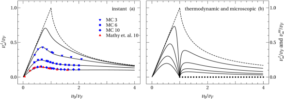
Figure 1: (Color online) Impurity’s end velocity shown as a function of the impurity’s initial velocity $v_{0}$. Left panel is for the instant injection protocol. Solid curves illustrate our analytic results for the impurity-gas interaction strength $\gamma=1,$ $3,$ $6,$ and $10$ (top to bottom). Blue down-triangles, boxes, and diamonds come from the stochastic Monte-Carlo simulations for $\gamma=3,$ $6,$ and $10$, respectively. Red up-triangles are the results for $\gamma=10$ obtained by combining Bethe ansatz and numerics in Ref. Mathy et al. (2012). Dashed curve corresponds to $v_{\infty}^{i}$ in the $\gamma\to 0$ limit. All curves converge to the $\gamma$-independent asymptotic form $v_{\infty}^{i}=2v_{F}^{2}/(3v_{0})$ in the large $v_{0}$ limit. Right panel is for the two adiabatic injection protocols: thermodynamic ($v_{\infty}^{t}$, solid lines) and microscopic ($v_{\infty}^{m}$, dotted lines). The values of $\gamma$ are the same as on the left panel. These two protocols lead to the same value of the end velocity of the impurity, $v_{\infty}^{t}=v_{\infty}^{m}$, for $v_{0}<v_{F}$, and therefore dotted lines are not plotted on top of the solid ones. However, $v_{\infty}^{t}$ is different from $v_{\infty}^{m}$ for $v_{0}>v_{F}$, where $v_{\infty}^{m}=0$ for all values of $\gamma$. The $\gamma\to 0$ limit of $v_{\infty}^{t}$ tends to the same dashed curve as in the left panel for all $v_{0}\neq v_{F}$, and $v^{t}_{\infty}=0$ for $v_{0}=v_{F}$. The units are set by the Fermi velocity $v_{F}=\pi\rho/m$.

The Hamiltonian of our system, consisting of an impurity of mass $m$ interacting with the gas particles of the same mass via a repulsive $\delta$-function potential reads

$$H=\sum_{j=1}^{N}\frac{P_{j}^{2}}{2m}+\frac{P_{\mathrm{imp}}^{2}}{2m}+\frac{\gamma\rho}{m}\sum_{j=1}^{N}\delta(x_{j}-x_{\mathrm{imp}}).$$ (1)

Here, $x_{j}$ ($P_{j}$) is the coordinate (momentum) of the $j$th gas particle, $j=1,\ldots,N,$ and $x_{\mathrm{imp}}$ ($P_{\mathrm{imp}}$) is that of the impurity. Planck’s constant $\hbar=1$ in our units, $\gamma$ represents the dimensionless strength of the impurity-gas repulsion, $\rho=N/L$ is the gas density, and $L$ is the system size. Our analytic results are obtained in the thermodynamic limit of large $N$ and $L$ at a fixed $\rho$ and zero temperature. We start the system out in the state

$$|\mathrm{FS},Q\rangle=c^{\dagger}_{\mathrm{imp}}(Q)|0\rangle\otimes|\mathrm{FS}\rangle,$$ (2)

where $c^{\dagger}_{\mathrm{imp}}(Q)$ creates an impurity plane wave with momentum $Q=mv_{0}$ from the vacuum $|0\rangle$, and a free spinless Fermi gas is in the Fermi sea ground state $|\mathrm{FS}\rangle$. We are interested in the impurity’s velocity at infinite time

$$v_{\infty}=\frac{1}{m}\lim_{t\to\infty}\langle\mathrm{FS},Q|P_{\mathrm{imp}}(t)|\mathrm{FS},Q\rangle,$$ (3)

where $P_{\mathrm{imp}}(t)$ is the impurity momentum operator in the Heisenberg representation.

We begin by considering an instant quench of the impurity-gas interaction. The time evolution of $P_{\mathrm{imp}}$ is determined by the Hamiltonian (1) with a given interaction strength $\gamma$:

$$v^{i}(t)=\frac{1}{m}\sum_{f_{\gamma},f^{\prime}_{\gamma}}e^{-it(E_{f_{\gamma}}-E_{f^{\prime}_{\gamma}})}\\ \times\langle f^{\prime}_{\gamma}|P_{\mathrm{imp}}|f_{\gamma}\rangle\langle\mathrm{FS},Q|f^{\prime}_{\gamma}\rangle\langle f_{\gamma}|\mathrm{FS},Q\rangle.$$ (4)

The double sum runs over complete sets of the eigenfunctions $|f_{\gamma}\rangle$ and $|f^{\prime}_{\gamma}\rangle$ of the Hamiltonian (1) having total momentum $Q$; $E_{f_{\gamma}}$ and $E_{f^{\prime}_{\gamma}}$ stand for the energies of these states. We denote the velocity from Eq. (3) obtained for the instant injection protocol as $v_{\infty}^{i}$. We have

$$v_{\infty}^{i}=\lim_{t\to\infty}v^{i}(t)=\frac{1}{m}\sum_{f_{\gamma}}\langle f_{\gamma}|P_{\mathrm{imp}}|f_{\gamma}\rangle|\langle f_{\gamma}|\mathrm{FS},Q\rangle|^{2}.$$ (5)

Here, we reduced the double sum from Eq. (4) to the single sum by assuming that only the terms with $E_{f_{\gamma}}=E_{f^{\prime}_{\gamma}}$ are relevant in the $t\to\infty$ limit. The states $|f_{\gamma}\rangle$ are found exactly by the Bethe ansatz technique for any finite $N$ and periodic boundary conditions McGuire (1965). Note that Eq. (1) is a particular case of the Gaudin-Yang model Gaudin (1967); Yang (1967). Evaluating the sum in Eq. (5) poses a separate challenge. We do this following the summation procedure developed in Refs. Gamayun et al. (2015, 2016), aiming at the thermodynamic limit, where boundary conditions play no role. The matrix elements $\langle f_{\gamma}|P_{\mathrm{imp}}|f_{\gamma}\rangle$ turn into an analytic function $\mathcal{P}(\Lambda)$ of a single argument $\Lambda$ in the thermodynamic limit. This way the sum in Eq. (5) is expressed as the double integral See Supplemental Material ,

$$\frac{v_{\infty}^{i}}{v_{F}}=-i\int_{-\infty}^{\infty}\frac{d\Lambda}{\pi}\mathcal{P}(\Lambda)\int_{0}^{\infty}dx\,\sin(xv_{0}/v_{F})F(\Lambda,x).$$ (6)

Here,

$$\mathcal{P}(\Lambda)=\frac{\Lambda}{\alpha}+\frac{1}{2\alpha}\frac{\ln\frac{1+(\alpha-\Lambda)^{2}}{1+(\alpha+\Lambda)^{2}}}{\arctan(\alpha-\Lambda)+\arctan(\alpha+\Lambda)},$$ (7)

where $\alpha=2\pi/\gamma$, and $k_{F}=\pi\rho$ and $v_{F}=k_{F}/m$ stands for the Fermi momentum and velocity, respectively. The function $F$ reads

$$F(\Lambda,x)=(h-1)\det(\hat{I}+\hat{V})+\det(\hat{I}+\hat{V}-\hat{W}).$$ (8)

The “det” symbol stands for the Fredholm determinant of the linear integral operators $\hat{V}$ and $\hat{W}$ defined on the domain $[-1,1]\times[-1,1]$ with the following kernels:

$$V(q,q^{\prime})=\frac{e_{+}(q)e_{-}(q^{\prime})-e_{-}(q)e_{+}(q^{\prime})}{q-q^{\prime}}$$ (9)

and

$$W(q,q^{\prime})=e_{+}(q)e_{+}(q^{\prime}).$$ (10)

The functions $e_{\pm}$ are defined as

$$e_{+}(q)=\frac{e(q)e^{-ixq/2}}{\sqrt{\pi}},\quad e_{-}(q)=\frac{e^{-ixq/2}}{\sqrt{\pi}},$$ (11)

where

$$e(q)=-\frac{e^{iqx}-\alpha h}{\Lambda+i-\alpha q},\quad h=\frac{1}{\alpha}e^{ix(\Lambda+i)/\alpha}.$$ (12)

Let us discuss the impurity’s stationary state in the $\gamma\to 0$ limit. Equation (6) implies See Supplemental Material

$$v_{\infty}^{i}=v_{0}-\theta(v_{0}-v_{F})\frac{v_{0}^{2}-v_{F}^{2}}{2v_{F}}\ln\frac{v_{0}+v_{F}}{v_{0}-v_{F}},\quad\gamma\to 0.$$ (13)

Here, $\theta$ is the Heaviside step function. This expression, shown with the dashed line in Fig. 1, has already been obtained in Ref. Burovski et al. (2014), by evaluating the sum in Eq. (5) with a technique special to the $\gamma\to 0$ limit. We stress that this limit is taken assuming the stationary state is already reached, which probably takes very long time. Thus, however small but finite $\gamma$ leads to impurity-gas scattering processes significantly modifying the stationary state of the impurity compared to the initial state (2) if $v_{0}>v_{F}$, and this does not happen for $v_{0}<v_{F}$. The density matrix $\varrho_{\infty}^{i}$ characterizing the impurity in the stationary state has not been found yet even in the $\gamma\to 0$ limit. We assume that the properties of this matrix are not affected by excitations in the gas caused by the equilibration process. Exploiting this assumption, we take $\varrho_{\infty}^{i}$ as a statistical mixture of the minimal energy states, which are given by $|\mathrm{FS},k\rangle$ with the total momentum lying in the interval $-k_{F}<k<k_{F}$:

$$\varrho_{\infty}^{i}=\sum_{|k|<k_{F}}n_{k}(Q)|\mathrm{FS},k\rangle\langle\mathrm{FS},k|,\quad\gamma\to 0.$$ (14)

The coefficients $n_{k}$ determine the impurity’s momentum distribution; they can be taken from Ref. Gamayun (2014):

$$n_{k}(Q)=\delta_{k,Q}+\frac{2\pi}{L}\frac{Q^{2}-k_{F}^{2}}{2k_{F}}\frac{\theta(Q-k_{F})}{(k-Q)^{2}}$$ (15)

for $-k_{F}\leq k\leq k_{F}$, and vanish outside this interval. Thus, Eq. (14) bridges exact many-body quantum mechanics and statistical physics, the latter not requiring full knowledge of the system’s dynamics for a description of a local microscopic object. We later use this equation to characterize the impurity injected adiabatically slow.

We now further examine the dependence of $v_{\infty}^{i}$ on the initial velocity. The large $v_{0}$ limit of Eq. (6) reads See Supplemental Material

$$v_{\infty}^{i}=\frac{2}{3}\frac{v_{F}^{2}}{v_{0}},\qquad v_{0}\gg v_{F}.$$ (16)

One can see from this expression that $v_{\infty}^{i}$ decays with increasing $v_{0}$, which may seem paradoxical. To understand such a behavior recall that a single scattering event of an impurity with momentum $Q$ and a gas particle with momentum $k$ yields the impurity’s reflection probability $R(k)=\gamma^{2}\rho^{2}/[(k-Q)^{2}+\gamma^{2}\rho^{2}]$. A toy model accounting for a single collision with gas particles having the Fermi sea momentum distribution, and ignoring that the time until such a collision takes place depends on the gas particle’s momentum, gives for the average impurity’s velocity

$$\tilde{v}^{i}=\frac{1}{m}\frac{\int_{-k_{F}}^{k_{F}}dk\,kR(k)}{\int_{-k_{F}}^{k_{F}}dk\,R(k)}.$$ (17)

This formula correctly reproduces Eqs. (13) and (16), illustrating that the dependence of the impurity’s end velocity on the initial one is non-monotonous.

For the intermediate values of $v_{0}$ and $\gamma$ we evaluate the Fredholm determinants entering Eq. (6) numerically See Supplemental Material using very efficient numerical procedure described in Ref. Bornemann (2010). The resulting plots are shown in Fig. 1(a) with the solid lines. We then verify that the time-dependent impurity velocity (4) found for a finite particle number $N$ numerically converges to $v_{\infty}^{i}$ given by Eq. (6) with increasing $t$ and $N$. We tackle the sum in Eq. (4) by the stochastic enumeration method Burovski et al. (2014); Malcomson (2016). It constructs a random walk in the space of the Bethe ansatz states $|f_{\gamma}\rangle$ based on the Metropolis algorithm Metropolis et al. (1953) with the Monte Carlo weight given by $|\langle f_{\gamma}|\mathrm{FS},Q\rangle|^{2}$, thus finding the most relevant states automatically. The results shown with the blue down-triangles, boxes, and diamonds in Fig. 1(a) are for $N=99$. The error bars are smaller than the size of the symbols; the positions of the symbols do not visibly change with further increase of $N$ . The deterministic truncation of the sum in Eq. (4) only retaining terms with up to three quasi-particle-hole excitations, employed in Ref. Mathy et al. (2012), leads to the results shown with the red up-triangles.

We now discuss the adiabatic injection protocols mentioned in the introduction. An important feature of the initial state (2) is its overlap with an eigenstate $|\tilde{f}_{\gamma}\rangle$ of the Hamiltonian (1) at a given total momentum $Q$ See Supplemental Material :

$$\langle\mathrm{FS},Q|\tilde{f}_{\gamma}\rangle\to 1,\quad N\to\infty\text{ after }\gamma\to 0.$$ (18)

Assuming that the ramp-up of $\gamma$ is sufficiently small for the system to stay close to $|\tilde{f}_{\gamma}\rangle$ at all times, we get for Eq. (3)

$$v_{\infty}^{m}=\frac{1}{m}\langle\tilde{f}_{\gamma}|P_{\mathrm{imp}}|\tilde{f}_{\gamma}\rangle.$$ (19)

The superscript “$m$” stands for microscopic, indicating that the above assumption exploits the structure of the excitation spectrum at the microscopic level. Using the Hellmann-Feynman theorem as explained in Ref. Knap et al. (2014) we get for Eq. (19)

$$v_{\infty}^{m}(Q)=\frac{\partial E_{\tilde{f}_{\gamma}}(Q)}{\partial Q},$$ (20)

where $E_{\tilde{f}_{\gamma}}(Q)$ is the energy of the state $|\tilde{f}_{\gamma}\rangle$.

In the case $v_{0}<v_{F}$ the state $|\tilde{f}_{\gamma}\rangle$ minimizes the Hamiltonian (1) at a given $Q$, and is non-degenerate. Hence, Eq. (18) holds for arbitrary $N$. The energy $E_{\tilde{f}_{\gamma}}$, denoted as $E_{\mathrm{min}}$, is shown with thick solid lines in Fig. 2(a) for several values of $\gamma$. This energy is quadratic for small $Q$, and $v_{\infty}^{m}=v_{0}m/m_{*}$ is the velocity of a particle-like excitation, a polaron with an effective mass $m_{*}$. We then compare $v_{\infty}^{i}$ and $v_{\infty}^{m}$ as $v_{0}\to 0$ and demonstrate in Fig. 2(b) that $v_{\infty}^{i}<v_{\infty}^{m}<v_{0}$ for any $\gamma>0$ See Supplemental Material . Thus, the stationary state formed past an instant injection with $v_{0}\to 0$ can not be described within the polaron theory approach suitable for the state formed past an adiabatic injection.

Figure 2: (a) The minimum of the excitation spectrum $E_{\mathrm{min}}(k)$ relative to $E_{\mathrm{min}}(0)$ for the impurity-gas interaction strength $\gamma=1,$ $3,$ $6,$ and $10$ (thick solid lines, in the order of decreasing magnitude). Dashed line corresponds to $E_{\mathrm{min}}(k)$ for $0\leq k\leq k_{F}$ at $\gamma=0$, which is the impurity’s kinetic energy. Thin solid line represents the minimum of the excitation spectrum of the free Fermi gas. (b) $v_{\infty}^{i}/v_{0}$ (dotted line) and $v_{\infty}^{i}/v_{\infty}^{m}$ (solid line) in the $v_{0}\to 0$ limit. Dashed horizontal line indicates $v_{\infty}^{i}/v_{\infty}^{m}=0.364\ldots$ in the $\gamma\to\infty$ limit.

In the case $v_{0}>v_{F}$ the initial state (2) is a degenerate non-minimal eigenstate of the Hamiltonian (1) at $\gamma=0$, and Eq. (18) holds only in the $N\to\infty$ limit. We identify $|\tilde{f}_{\gamma}\rangle$ rigorously by examining the Bethe ansatz solution, and Eq. (20) gives See Supplemental Material

$$v_{\infty}^{m}=0,\quad v_{0}>v_{F}$$ (21)

regardless of the value of $\gamma$. We thus found that sufficiently slow ramp-ups of the interaction lead to a complete stop of the impurity initiated in the state (2) whose energy is above the minimal excitation energy of a free Fermi gas by a finite amount.

The thermodynamically large system has vanishing level spacing. This poses the problem of the validity of Eq. (19) since arbitrarily slow ramp-up of the interaction strength could possibly drive the system away from the state $|\tilde{f}_{\gamma}\rangle$. Let us impose a thermodynamic adiabaticity condition, more relaxed than the microscopic one. It is realized if the rate of change of the interaction constant $\gamma$ is smaller than the macroscopic energy scales of the system. We then exploit an assumption of separation of time-scales. The change of $\gamma$ from zero to a small finite value is viewed as an instant quench driving the system away from the state $|\tilde{f}_{\gamma=0}\rangle$, though being slow enough to let the impurity reach the stationary state given by the density matrix (14). Each term of $\varrho_{\infty}^{i}$ is the projector onto a state given by Eq. (2), with the momentum $|k|<k_{F}$. A subsequent slow change of $\gamma$ is assumed to make each of those states follow its own path of the microscopic adiabatic evolution, and we get for the end velocity of the impurity in the thermodynamically adiabatic injection protocol

$$v_{\infty}^{t}(Q)=\sum_{|k|<k_{F}}n_{k}(Q)v_{\infty}^{m}(k),$$ (22)

where $n_{k}$ is given by Eq. (15), and $v_{\infty}^{m}$ by Eq. (20). One can see that $v_{\infty}^{t}$ and $v_{\infty}^{i}$, illustrated in Fig. 1, only coincide in the $\gamma\to 0$ and $\gamma\to\infty$ limits. Note also, that for any $v_{0}$, $v_{\infty}^{i}$ is smaller than the maximum of $v_{\infty}^{t}$ with respect to $Q$. This proves a cojecture from Ref. Knap et al. (2014).

We recapitulate that the difference between the microscopically and thermodynamically adiabatic injection protocols can be seen by comparing $v_{\infty}^{m}$ and $v_{\infty}^{t}$, given by Eqs. (19) and (22), respectively. Such a difference arises for $v_{0}>v_{F}$, in which case $v_{\infty}^{m}$ vanishes, Eq. (21), and $v_{\infty}^{t}$ is non-zero, as shown in Fig. 1(b). Determining the rate of change of $\gamma$ for which a transition from $v_{\infty}^{m}$ to $v_{\infty}^{t}$ happens in a large but finite system is a challenging open problem. The density of states of a free Fermi gas grows exponentially with $N$ for any value of the energy that is above the minimum of the excitation spectrum by a finite amount Bohr and Mottelson (1998). Given such a rapid growth, this rate probably diminishes very fast with $N$. However, existing quantitative theories of adiabaticity breaking are not based on the properties of the density of states Lychkovskiy et al. (2016, 2017), and their implementation for our problem requires a separate study.

In summary, we performed a quantitative study of the impurity’s stationary state for one-dimensional Fermi gas (the results for the Tonks-Girardeau gas of strongly repulsive bosons will be identical Mathy et al. (2012)). Our analysis shows that (i) The stationary state of an impurity moving through the gas is not completely determined by the kinematic constraints of Landau approach to superfluidity. In particular, the value of the impurity’s end velocity depends on the initial velocity $v_{0}$, as well as on how the impurity-gas interaction strength $\gamma$ is ramped up with time. We demonstrated that a quantitative study is necessary to understand when this value is zero. In other words, neither zero nor non-zero value of the impurity’s end velocity seem to be protected by symmetry or kinematic constraints in case of a general injection protocol. Note that our results are consistent with the assumption that the Landau critical velocity (that is, the velocity of sound, equal to $v_{F}$ for our model) is an upper bound for the impurity’s end velocity. (ii) If the impurity’s initial kinetic energy is above the minimum of the excitation spectrum of the Fermi gas, that is $v_{0}>v_{F}$, the microscopic adiabaticity condition (the ramp-up of $\gamma$ is smaller than the level spacing) and the thermodynamic one (the ramp-up of $\gamma$ is larger than the level spacing but smaller than the Fermi energy) lead to different impurity’s steady states and end velocities. Since (i) and (ii) are qualitative statements, they hold for one-dimensional gases with arbitrary interactions. Finally, our numerical simulations for systems having up to $100$ particles suggest that the effects we discuss should be observable in existing ultracold gas experiments. For example, the setup of Meinert et al. (2016) consists of a few (between one and three) impurities and about $60$ host atoms of cesium confined in a one-dimensional trap. The final state of the impurity accelerated by a constant external force has been measured. A modification of this setup in which the external force can be switched on and off would make the phenomena discussed in this Letter experimentally accessible.