$B^{\ast}$ ${\to}$ $\overline{D}D$ decays with perturbative QCD approach

Abstract

The nonleptonic two-body $B^{\ast}$ ${\to}$ $\overline{D}D$ weak decays are studied phenomenologically with the perturbative QCD factorization approach. It is found that the $B_{s}^{{\ast}0}$ ${\to}$ $D_{s}^{-}D_{s}^{+}$, $B_{d}^{{\ast}0}$ ${\to}$ $D_{d}^{-}D_{s}^{+}$, and $B_{u}^{{\ast}+}$ ${\to}$ $\overline{D}_{u}^{0}D_{s}^{+}$ decays have branching ratios ${\gtrsim}$ $10^{-9}$, and might be promisingly measurable at the running LHC and forthcoming SuperKEKB experiments in the future.

I Introduction

The $B_{q}^{\ast}$ mesons, consisting of $\bar{b}q$ pair with $q$ $=$ $u$, $d$ and $s$, are spin-triplet ground vector states with definite spin-parity quantum numbers of $J^{P}$ $=$ $1^{-}$ pdg . Because the mass splittings $m_{B_{q}^{\ast}}$ $-$ $m_{B_{q}}$ ${\lesssim}$ 50 MeV pdg are much smaller than the mass of the lightest pion meson, the $B_{q}^{\ast}$ meson decays dominantly into the ground pseudoscalar $B_{q}$ meson through the electromagnetic interaction. Besides, the $B_{q}^{\ast}$ mesons can also decay via the bottom-changing transition induced by the weak interaction within the standard model (SM). Because of the strong phase-space suppression from their dominant magnetic dipole (M1) transition $B_{q}^{\ast}$ ${\to}$ $B_{q}{\gamma}$, the lifetime of the $B_{q}^{\ast}$ meson is of the order of $10^{-17}$ second or less, which, in general, is too short to enable the $B_{q}^{\ast}$ meson to experience the weak disintegration 1509.05049 . The $B_{q}^{\ast}$ weak decays have not actually attracted much attention yet. Until now, there has been no experimental report and few theoretical works concentrating on the $B_{q}^{\ast}$ weak decay, subject to the relatively inadequate statistics on the $B_{q}^{\ast}$ mesons. Fortunately, the high luminosities and large production rates at LHC and the forthcoming SuperKEKB are promising, and the rapid accumulation of more and more $B_{q}^{\ast}$ data samples is expected to be possible. Some $B_{q}^{\ast}$ weak decay modes might be detected and investigated in the future, which undoubtedly makes the $B_{q}^{\ast}$ mesons another a vibrant arena for testing the Cabibbo-Kabayashi-Maskawa (CKM) picture for $CP$-violating phenomena, examining our comprehension of the underlying dynamical factorization mechanism, and so on. In addition, heavy quark symmetry relates hadronic transition matrix elements (HTME) of the $B_{q}^{\ast}$ and $B_{q}$ weak decays. The interplay between the $B_{q}^{\ast}$ and $B_{q}$ weak decays could prove useful information to overconstraint parameters in the SM, and might shed some fresh light on various anomalies in $B$ decays.

The purely leptonic decays $B_{q}^{\ast}$ ${\to}$ ${\ell}^{+}{\ell}^{-}$ induced by the flavor-changing neutral currents have been studied recently in the SM 1509.05049 ; 1601.03386 . The semileptonic and nonleptonic $B_{q}^{\ast}$ decays have been investigated also in the SM 1605.01630 ; 1605.01629 ; 1605.01631 ; 1606.09071 , where the transition form factors are evaluated with the Wirbel-Stech-Bauer approach zpc29 , and the nonfactorizable corrections to HTME are considered 1605.01629 ; 1605.01631 based on the collinear-based and QCD-improved factorization (QCDF) approach qcdf1 ; qcdf2 ; qcdf3 ; plb.509.263 ; prd64.014036 . In this paper, we will study the nonleptonic $B_{q}^{\ast}$ decay into the pseudoscalar charmed-meson pair $\overline{D}D$ with the perturbative QCD factorization (pQCD) approach pqcd1 ; pqcd2 ; pqcd3 , just to provide a ready reference for the future experimental research. In addition, as is well known, the production ratio for the $B_{q}^{\ast}$ meson is comparable with that for the $B_{q}$ meson (see Table 3), the $B_{q}^{\ast}$ and $B_{q}$ mesons have nearly equal mass. Hence, the study of the $B_{q}^{\ast}$ ${\to}$ $\overline{D}D$ decays will undoubtedly be helpful to the experimental background analysis on the $B_{q}$ ${\to}$ $\overline{D}D$ decays.

This paper is organized as follows. The theoretical framework and amplitudes for $B_{q}^{\ast}$ ${\to}$ $\overline{D}D$ decays with pQCD approach are given in section II. Section III is devoted to numerical results and discussion. The final section is a summary.

II theoretical framework

II.1 The effective Hamiltonian

The effective Hamiltonian describing the $B_{q}^{\ast}$ ${\to}$ $\overline{D}D$ weak decay is written as 9512380

$${\cal H}_{\rm eff}\,=\,\frac{G_{F}}{\sqrt{2}}\sum\limits_{q=d,s}\Big{\{}\sum\limits_{p=u,c}V_{pb}^{\ast}V_{pq}\sum\limits_{i=1}^{2}C_{i}({\mu})\,Q_{i}({\mu})-V_{tb}^{\ast}V_{tq}\,\sum\limits_{k=3}^{10}C_{k}({\mu})\,Q_{k}({\mu})\Big{\}}+{\rm h.c.},$$ (1)

where the Fermi coupling constant $G_{F}$ ${\simeq}$ $1.166{\times}10^{-5}\,{\rm GeV}^{-2}$ pdg ; $V_{pb}^{\ast}V_{pq}$ and $V_{tb}^{\ast}V_{tq}$ are the CKM factors; The scale ${\mu}$ factorizes the physical contributions into two parts: the Wilson coefficients $C_{i}$ and the local four-fermion operators $Q_{i}$. The operators are defined as follows.

$$Q_{1} = (\bar{b}_{\alpha}\,p_{\alpha})_{V-A}\,(\bar{p}_{\beta}\,q_{\beta})_{V-A},\qquad\qquad\quad\ \ Q_{2}\ =\ (\bar{b}_{\alpha}\,p_{\beta})_{V-A}\,(\bar{p}_{\beta}\,q_{\alpha})_{V-A},$$ (2)

$$Q_{3} = \sum\limits_{q^{\prime}}\,(\bar{b}_{\alpha}\,q_{\alpha})_{V-A}\,(\bar{q}^{\prime}_{\beta}\,q^{\prime}_{\beta})_{V-A},\qquad\qquad Q_{4}\ =\ \sum\limits_{q^{\prime}}\,(\bar{b}_{\alpha}\,q_{\beta})_{V-A}\,(\bar{q}^{\prime}_{\beta}\,q^{\prime}_{\alpha})_{V-A},$$ (3)

$$Q_{5} = \sum\limits_{q^{\prime}}\,(\bar{b}_{\alpha}\,q_{\alpha})_{V-A}\,(\bar{q}^{\prime}_{\beta}\,q^{\prime}_{\beta})_{V+A},\qquad\qquad Q_{6}\ =\ \sum\limits_{q^{\prime}}\,(\bar{b}_{\alpha}\,q_{\beta})_{V-A}\,(\bar{q}^{\prime}_{\beta}\,q^{\prime}_{\alpha})_{V+A},$$ (4)

$$Q_{7} = \sum\limits_{q^{\prime}}\,\frac{3}{2}\,Q_{q^{\prime}}\,(\bar{b}_{\alpha}\,q_{\alpha})_{V-A}\,(\bar{q}^{\prime}_{\beta}\,q^{\prime}_{\beta})_{V+A},\quad\ Q_{8}\ =\ \sum\limits_{q^{\prime}}\,\frac{3}{2}\,Q_{q^{\prime}}\,(\bar{b}_{\alpha}\,q_{\beta})_{V-A}\,(\bar{q}^{\prime}_{\beta}\,q^{\prime}_{\alpha})_{V+A},$$ (5)

$$Q_{9} = \sum\limits_{q^{\prime}}\,\frac{3}{2}\,Q_{q^{\prime}}\,(\bar{b}_{\alpha}\,q_{\alpha})_{V-A}\,(\bar{q}^{\prime}_{\beta}\,q^{\prime}_{\beta})_{V-A},\quad Q_{10}\ =\ \sum\limits_{q^{\prime}}\,\frac{3}{2}\,Q_{q^{\prime}}\,(\bar{b}_{\alpha}\,q_{\beta})_{V-A}\,(\bar{q}^{\prime}_{\beta}\,q^{\prime}_{\alpha})_{V-A},$$ (6)

where $Q_{1,2}$ are tree operators arising from the $W$-boson exchange; $Q_{3,{\cdots},6}$ and $Q_{7,{\cdots},10}$ are called the QCD and electroweak penguin operators, respectively; $(\bar{q}_{1}\,q_{2})_{V{\pm}A}$ ${\equiv}$ $\bar{q}_{1}\,{\gamma}_{\mu}(1{\pm}{\gamma}_{5})\,q_{2}$; ${\alpha}$ and ${\beta}$ are color indices; $q^{\prime}$ denotes all the active quarks at the scale of ${\cal O}(m_{b})$, i.e., $q^{\prime}$ $=$ $u$, $d$, $c$, $s$, $b$; and $Q_{q^{\prime}}$ is the electric charge of quark $q^{\prime}$ in the unit of ${|}e{|}$.

The Wilson coefficients $C_{i}(\mu)$, which summarize the physical contributions above the scale of ${\mu}$, have been properly calculated at the next-to-leading order with the renormalization group equation assisted perturbation theory 9512380 . Due to the presence of long-distance QCD effects and the entanglement of nonperturbative and perturbative shares, the main obstacle to evaluate the $B_{q}^{(\ast)}$ weak decays is the treatment of physical contributions below the scale of ${\mu}$ which are included in the HTME of local operators.

II.2 Hadronic matrix elements

Some phenomenological models have recently been developed to improve the sketchy treatment with naive factorization scheme npb133 ; zpc34 . These models are generally based on the Lepage-Brodsky approach prd22 and some power counting rules in parameters of ${\alpha}_{s}$ and ${\Lambda}_{\rm QCD}/m_{Q}$ (where ${\alpha}_{s}$ is the strong coupling, ${\Lambda}_{\rm QCD}$ is the QCD characteristic scale, and $m_{Q}$ is the mass of a heavy quark), and express the HTME as a convolution integral of universal wave functions and hard scattering subamplitudes, such as the QCDF approach qcdf1 ; qcdf2 ; qcdf3 , pQCD approach pqcd1 ; pqcd2 ; pqcd3 , the soft and collinear effective theory scet1 ; scet2 ; scet3 ; scet4 , and so on, which have been extensively employed in the interpretation of the $B$ weak decays. To wipe out the endpoint singularities appearing in the collinear approximation qcdf1 ; qcdf2 ; qcdf3 , it is suggested by the pQCD approach pqcd1 ; pqcd2 ; pqcd3 that the transverse momentum $k_{T}$ of valence quarks should be retaken, and a Sudakov factor should be introduced for each wave function to further suppress the soft contributions and make the hard scattering more perturbative. Finally, a decay amplitude is written as a multidimensional integral of many parts pqcd2 ; pqcd3 , including the Wilson coefficients $C_{i}$, the heavy quark decay subamplitudes ${\cal H}$, and the universal wave functions ${\Phi}$,

$${\cal A}\,{\sim}\,\sum_{i}{\int}{\prod_{j}}dk_{j}\,C_{i}(t)\,{\cal H}_{i}(t,k_{j})\,{\Phi}_{j}(k_{j})\,e^{-S_{j}},$$ (7)

where $t$ is a typical scale; $k_{j}$ is the momentum of a valence quark; $e^{-S_{j}}$ is a Sudakov factor.

II.3 Kinematic variables

The light-cone variables in the rest frame of the $B^{\ast}$ meson are defined as follows.

$$p_{B^{\ast}}\,=\,p_{1}\,=\,\frac{m_{1}}{\sqrt{2}}(1,1,0),$$ (8)

$$p_{\overline{D}}\,=\,p_{2}\,=\,(p_{2}^{+},p_{2}^{-},0),$$ (9)

$$p_{D}\,=\,p_{3}\,=\,(p_{3}^{-},p_{3}^{+},0),$$ (10)

$$k_{i}\,=\,x_{i}\,p_{i}+(0,0,\vec{k}_{i{T}}),$$ (11)

$$p_{i}^{\pm}\,=\,(E_{i}\,{\pm}\,p)/\sqrt{2},$$ (12)

$${\epsilon}_{B^{\ast}}^{{\parallel}}\,=\,\frac{1}{\sqrt{2}}(-1,1,0),$$ (13)

$$s\,=\,2\,p_{2}{\cdot}p_{3},$$ (14)

$$t\,=\,2\,p_{1}{\cdot}p_{2}\,=\ 2\,m_{1}\,E_{2},$$ (15)

$$u\,=\,2\,p_{1}{\cdot}p_{3}\,=\ 2\,m_{1}\,E_{3},$$ (16)

$$s\,t+s\,u-t\,u-4\,m_{1}^{2}\,p^{2}\ =\ 0,$$ (17)

where the subscripts $i$ $=$ $1$, $2$, $3$ of variables (energy $E_{i}$, momentum $p_{i}$ and mass $m_{i}$) correspond to $B^{\ast}$, $\overline{D}$ and $D$ mesons, respectively; $k_{i}$ is the momentum of the valence quark with the longitudinal momentum fraction $x_{i}$ and the transverse momentum $\vec{k}_{iT}$; ${\epsilon}_{B^{\ast}}^{{\parallel}}$ is the longitudinal polarization vector; $p$ is the momentum of the final states; $s$, $t$ and $u$ are the Lorentz invariant parameters. The notation is displayed in Fig.2.

II.4 Wave functions

Wave functions are the basic input parameters with the pQCD approach. Although wave functions contain soft and nonperturbative contributions, they are universal, i.e., process independent. Wave functions and/or distribution amplitudes (DAs) determined by nonperturbative methods or extracted from data, can be employed here to make predictions.

Following the notations in Refs. npb529 ; prd65 ; plb752sun ; ijmpa31yang , HTME of the diquark operators is defined as

$${\langle}0{|}\bar{b}_{i}(0)q_{j}(z){|}B^{\ast}(p,{\epsilon}^{\parallel}){\rangle}\,=\,\frac{f_{B^{\ast}}}{4}{\int}d^{4}k\,e^{-ik{\cdot}z}\Big{\{}\!\!\not{\!\epsilon}^{\parallel}\,\Big{[}m_{B^{\ast}}\,{\Phi}_{B^{\ast}}^{v}(k)-\!\!\not{p}\,{\Phi}_{B^{\ast}}^{t}(k)\Big{]}\Big{\}}_{ji},$$ (18)

$${\langle}\overline{D}(p){|}c_{i}(0)\bar{q}_{j}(z){|}0{\rangle}\,=\,\frac{i\,f_{D}}{4}{\int}d^{4}k\,e^{+ik{\cdot}z}\,\Big{\{}{\gamma}_{5}\,\Big{[}\!\!\not{p}\,{\Phi}_{\bar{D}}^{a}(k)+m_{\bar{D}}\,{\Phi}_{\bar{D}}^{p}(k)\Big{]}\Big{\}}_{ji},$$ (19)

where $f_{B^{\ast}}$ and $f_{D}$ are decay constants; the wave functions ${\Phi}_{B^{\ast}}^{v}$ and ${\Phi}_{\bar{D}}^{a}$ are twist-2; and ${\Phi}_{B^{\ast}}^{t}$ and ${\Phi}_{\bar{D}}^{p}$ are twist-3. Due to the kinematic relation ${\epsilon}_{B^{\ast}}^{\perp}{\cdot}p_{i}$ $=$ $0$, the transversely polarized $B^{\ast}$ meson contributes nothing to the amplitudes for the $B^{\ast}$ ${\to}$ $\overline{D}D$ decays. The expressions for DAs of the $B^{\ast}$ and $D$ mesons are plb752sun ; ijmpa31yang

$${\phi}_{B^{\ast}}^{v}(x)=A\,x\,\bar{x}\,{\exp}\Big{\{}-\frac{\bar{x}\,m_{q}^{2}+x\,m_{b}^{2}}{8\,{\omega}_{1}^{2}\,x\,\bar{x}}\Big{\}},$$ (20)

$${\phi}_{B^{\ast}}^{t}(x)=B\,(\bar{x}-x)^{2}\,{\exp}\Big{\{}-\frac{\bar{x}\,m_{q}^{2}+x\,m_{b}^{2}}{8\,{\omega}_{1}^{2}\,x\,\bar{x}}\Big{\}},$$ (21)

$${\phi}_{\bar{D}}^{a}(x)=C\,x\,\bar{x}\,{\exp}\Big{\{}-\frac{\bar{x}\,m_{q}^{2}+x\,m_{c}^{2}}{8\,{\omega}_{2}^{2}\,x\,\bar{x}}\Big{\}},$$ (22)

$${\phi}_{\bar{D}}^{p}(x)=D\,{\exp}\Big{\{}-\frac{\bar{x}\,m_{q}^{2}+x\,m_{c}^{2}}{8\,{\omega}_{2}^{2}\,x\,\bar{x}}\Big{\}},$$ (23)

where $x$ and $\bar{x}$ (${\equiv}$ $1$ $-$ $x$) are the parton momentum fractions; ${\omega}_{i}$ determines the average transverse momentum of partons and ${\omega}_{i}$ ${\simeq}$ $m_{i}\,{\alpha}_{s}(m_{i})$; parameters $A$, $B$, $C$, $D$ are the normalization coefficients satisfying the conditions

$${\int}_{0}^{1}dx\,{\phi}_{B^{\ast}}^{v,t}(x)=1,$$ (24)

$${\int}_{0}^{1}dx\,{\phi}_{\bar{D}}^{a,p}(x)=1.$$ (25)

In fact, there are many phenomenological models of DAs for the charmed meson, for example, some of them have been listed by Eq.(30) in Ref.prd78.014018 . One of the favorable models from the experimental data within the pQCD framework has the expression prd78.014018

$${\phi}_{D}(x)=6\,x\bar{x}\,\big{\{}1+C_{D}(1-2x)\big{\}},$$ (26)

where parameter $C_{D}$ $=$ $0.5$ for the $D_{u,d}$ meson, and $C_{D}$ $=$ $0.4$ for the $D_{s}$ meson. In the actual calculation prd78.014018 ; prd81.034006 ; jpg31.273 ; jpg37 , there is no distinction between twist-2 and twist-3 DAs.

The shape lines of the normalized DAs ${\phi}_{B^{\ast}}^{v,t}(x)$ and ${\phi}_{D}^{a,p}(x)$ are illustrated in Fig.1. It is clearly seen from Fig.1 that (1) the shape lines of DAs in Eqs.(20)-(23) have a broad peak in the small $x$ regions, which is generally consistent with an ansatz in which a light quark carries fewer parton momentum fractions than a heavy quark in a heavy-light system. (2) Due to the suppression from exponential functions, the DAs of Eqs.(20)-(23) converge quickly to zero at endpoint $x$, $\bar{x}$ ${\to}$ $0$, which supplies the soft contributions with an effective cutoff. (3) The flavor symmetry breaking effects, and especially the distinction between different the twist DAs, are highlighted, compared with the nearly symmetric distribution Eq.(26).

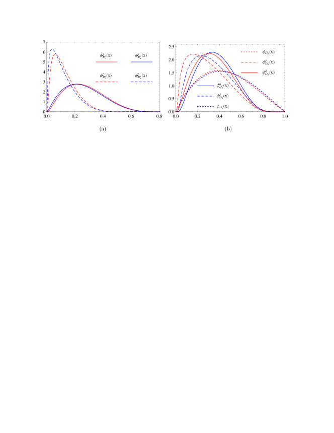
Figure 1: The distributions of DAs ${\phi}_{B^{\ast}}^{v,t}(x)$ [Eqs.(20,21)], ${\phi}_{D}^{a,p}(x)$ [Eqs.(22,23)], and ${\phi}_{D}(x)$ [Eq.(26)].

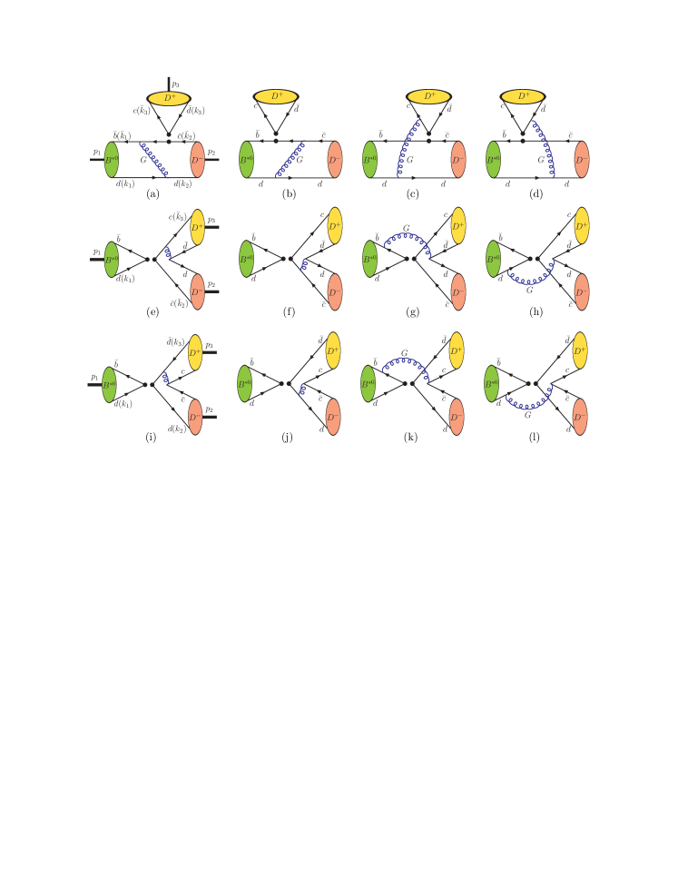
Figure 2: Feynman diagrams for $B^{{\ast}0}$ ${\to}$ $D^{+}D^{-}$ decay, where (a,b) are the factorizable emission topologies, (c,d) are the nonfactorizable emission topologies, (e,f,i,j) are the factorizable annihilation topologies, and (g,h,k,l) are the nonfactorizable annihilation topologies.

II.5 Decay amplitudes

The Feynman diagrams for the $B^{{\ast}0}$ ${\to}$ $D^{+}D^{-}$ decay with the pQCD approach are shown in Fig.2, including the factorizable emission topologies (a,b) where one gluon links with the initial and the recoiled states, the nonfactorizable emission topologies (c,d) where one gluon is exchanged between the spectator quark and the emitted states, the factorizable annihilation topologies (e,f,i,j) where one gluon is conjoined with the final states, and the nonfactorizable annihilation topologies (g,h,k,l) where one gluon is transmitted between the initial and the final states.

Generally, the amplitudes for the factorizable emission topologies in Fig.2(a,b) can be written as the $D$ meson decay constant and the space-like $B^{\ast}$ ${\to}$ $D$ transition form factor, and the amplitudes for the factorizable annihilation topologies in Fig.2(e,f,i,j) can be written as the $B^{\ast}$ meson decay constant and the time-like transition form factor between two charmed mesons. The amplitudes for the nonfactorizable topologies have more complicated structures, and can be written as the convolution integral of all participating meson wave functions. Compared with the contributions of the emission topologies in Fig.2(a-d), the contributions of the annihilation topologies in Fig.2(e-l) are assumed to be power suppressed, as stated in Ref.qcdf2 . In addition, different topologies have different scales. The gluons of the emission topologies in Fig.2(a-d) are time-like, while the gluons of the annihilation topologies in Fig.2(e-l) are space-like. The gluon virtuality of creating a pair of heavy charm quarks from the vacuum for the annihilation topologies in Fig.2(i-l), $k_{g}^{2}$ ${\geq}$ $(2m_{c})^{2}$, should be much larger than that of producing a pair of light quarks for the annihilation topologies in Fig.2(e-h). Thus, it is not hard to figure out that the contributions of the annihilation topologies in Fig.2(i-l) might be very small relative to the others, because of the nature of the asymptotic freedom of the QCD at the unltrahigh energy.

After a straightforward calculation, the amplitudes for the $B_{q}^{\ast}$ ${\to}$ $\overline{D}D$ decays are expressed as below.

$${\cal A}(B^{{\ast}+}{\to}\overline{D}^{0}D_{q}^{+})$$ (27)

$$= {\cal F}\,\Big{\{}V_{cb}^{\ast}\,V_{cq}\,\Big{[}a_{1}\,{\cal A}_{a+b}^{LL}+C_{2}\,{\cal A}_{c+d}^{LL}\Big{]}+V_{ub}^{\ast}\,V_{uq}\,\Big{[}a_{1}\,{\cal A}_{i+j}^{LL}+C_{2}\,{\cal A}_{k+l}^{LL}\Big{]}$$

$$\quad-V_{tb}^{\ast}\,V_{tq}\,\Big{[}(a_{4}+a_{10})\,{\cal A}_{a+b+i+j}^{LL}+(a_{6}+a_{8})\,{\cal A}_{a+b}^{SP}$$

$$\qquad\qquad+\ (C_{3}+C_{9})\,{\cal A}_{c+d+k+l}^{LL}+(C_{5}+C_{7})\,{\cal A}_{c+d+k+l}^{SP}\Big{]}\Big{\}},$$

$${\cal A}(B_{q}^{{\ast}0}{\to}\overline{D}^{0}D^{0})$$ (28)

$$= {\cal F}\,\Big{\{}V_{cb}^{\ast}\,V_{cq}\,\Big{[}a_{2}\,{\cal A}_{e+f}^{LL}+C_{1}\,{\cal A}_{g+h}^{LL}\Big{]}+V_{ub}^{\ast}\,V_{uq}\,\Big{[}a_{2}\,{\cal A}_{i+j}^{LL}+C_{1}\,{\cal A}_{k+l}^{LL}\Big{]}$$

$$\quad-V_{tb}^{\ast}\,V_{tq}\,\Big{[}(a_{3}+a_{9})\,{\cal A}_{e+f+i+j}^{LL}+(a_{5}+a_{7})\,{\cal A}_{e+f+i+j}^{LR}$$

$$\qquad\ \ \quad+\ (C_{4}+C_{10})\,{\cal A}_{g+h+k+l}^{LL}+(C_{6}+C_{8})\,{\cal A}_{g+h+k+l}^{LR}\Big{]}\Big{\}},$$

$${\cal A}(B_{q}^{{\ast}0}{\to}D_{q}^{-}D_{q}^{+})$$ (29)

$$= {\cal F}\,\Big{\{}V_{cb}^{\ast}\,V_{cq}\,\Big{[}a_{1}\,{\cal A}_{a+b}^{LL}+C_{2}\,{\cal A}_{c+d}^{LL}+a_{2}\,{\cal A}_{e+f}^{LL}+C_{1}\,{\cal A}_{g+h}^{LL}\Big{]}$$

$$\quad-V_{tb}^{\ast}\,V_{tq}\,\Big{[}(a_{4}+a_{10})\,{\cal A}_{a+b}^{LL}+(a_{6}+a_{8})\,{\cal A}_{a+b}^{SP}+(a_{3}+a_{9})\,{\cal A}_{e+f}^{LL}$$

$$\quad+\ (C_{3}+C_{9})\,{\cal A}_{c+d}^{LL}+(C_{5}+C_{7})\,{\cal A}_{c+d}^{SP}+(C_{4}+C_{10})\,{\cal A}_{g+h}^{LL}$$

$$\quad+\ (a_{5}-\frac{1}{2}\,a_{7})\,{\cal A}_{i+j}^{LR}+(C_{5}-\frac{1}{2}\,C_{7})\,{\cal A}_{k+l}^{SP}+(C_{6}-\frac{1}{2}\,C_{8})\,{\cal A}_{k+l}^{LR}$$

$$\quad+\ (a_{5}+a_{7})\,{\cal A}_{e+f}^{LR}+(a_{3}+a_{4}-\frac{1}{2}\,a_{9}-\frac{1}{2}\,a_{10})\,{\cal A}_{i+j}^{LL}$$

$$\quad+\ (C_{6}+C_{8})\,{\cal A}_{g+h}^{LR}+(C_{3}+C_{4}-\frac{1}{2}\,C_{9}-\frac{1}{2}\,C_{10})\,{\cal A}_{k+l}^{LL}\Big{]}\Big{\}},$$

$${\cal A}(B_{d}^{{\ast}0}{\to}D^{-}D_{s}^{+})$$ (30)

$$= {\cal F}\,\Big{\{}V_{cb}^{\ast}\,V_{cs}\,\Big{[}a_{1}\,{\cal A}_{a+b}^{LL}+C_{2}\,{\cal A}_{c+d}^{LL}\Big{]}-V_{tb}^{\ast}\,V_{ts}\,\Big{[}(a_{4}+a_{10})\,{\cal A}_{a+b}^{LL}$$

$$\quad+\ (a_{4}-\frac{1}{2}\,a_{10})\,{\cal A}_{i+j}^{LL}+(C_{3}-\frac{1}{2}\,C_{9})\,{\cal A}_{k+l}^{LL}+(C_{5}-\frac{1}{2}\,C_{7})\,{\cal A}_{k+l}^{SP}$$

$$\quad+\ (a_{6}+a_{8})\,{\cal A}_{a+b}^{SP}+(C_{3}+C_{9})\,{\cal A}_{c+d}^{LL}+(C_{5}+C_{7})\,{\cal A}_{c+d}^{SP}\Big{]}\Big{\}},$$

$${\cal A}(B_{s}^{{\ast}0}{\to}D_{s}^{-}D^{+})$$ (31)

$$= {\cal F}\,\Big{\{}V_{cb}^{\ast}\,V_{cd}\,\Big{[}a_{1}\,{\cal A}_{a+b}^{LL}+C_{2}\,{\cal A}_{c+d}^{LL}\Big{]}-V_{tb}^{\ast}\,V_{td}\,\Big{[}(a_{4}+a_{10})\,{\cal A}_{a+b}^{LL}$$

$$\quad+\ (a_{4}-\frac{1}{2}\,a_{10})\,{\cal A}_{i+j}^{LL}+(C_{3}-\frac{1}{2}\,C_{9})\,{\cal A}_{k+l}^{LL}+(C_{5}-\frac{1}{2}\,C_{7})\,{\cal A}_{k+l}^{SP}$$

$$\quad+\ (a_{6}+a_{8})\,{\cal A}_{a+b}^{SP}+(C_{3}+C_{9})\,{\cal A}_{c+d}^{LL}+(C_{5}+C_{7})\,{\cal A}_{c+d}^{SP}\Big{]}\Big{\}},$$

$${\cal A}(B_{d}^{{\ast}0}{\to}D_{s}^{-}D_{s}^{+})$$ (32)

$$= {\cal F}\,\Big{\{}V_{cb}^{\ast}\,V_{cd}\,\Big{[}a_{2}\,{\cal A}_{e+f}^{LL}+C_{1}\,{\cal A}_{g+h}^{LL}\Big{]}-V_{tb}^{\ast}\,V_{td}\,\Big{[}(a_{3}+a_{9})\,{\cal A}_{e+f}^{LL}$$

$$\quad+\ (a_{5}+a_{7})\,{\cal A}_{e+f}^{LR}+(C_{4}+C_{10})\,{\cal A}_{g+h}^{LL}+(C_{6}+C_{8})\,{\cal A}_{g+h}^{LR}$$

$$\quad+\ (a_{3}-\frac{1}{2}\,a_{9})\,{\cal A}_{i+j}^{LL}+(C_{4}-\frac{1}{2}\,C_{10})\,{\cal A}_{k+l}^{LL}$$

$$\quad+\ (a_{5}-\frac{1}{2}\,a_{7})\,{\cal A}_{i+j}^{LR}+(C_{6}-\frac{1}{2}\,C_{8})\,{\cal A}_{k+l}^{LR}\Big{]}\Big{\}},$$

$${\cal A}(B_{s}^{{\ast}0}{\to}D^{-}D^{+})$$ (33)

$$= {\cal F}\,\Big{\{}V_{cb}^{\ast}\,V_{cs}\,\Big{[}a_{2}\,{\cal A}_{e+f}^{LL}+C_{1}\,{\cal A}_{g+h}^{LL}\Big{]}-V_{tb}^{\ast}\,V_{ts}\,\Big{[}(a_{3}+a_{9})\,{\cal A}_{e+f}^{LL}$$

$$\quad+\ (a_{5}+a_{7})\,{\cal A}_{e+f}^{LR}+(C_{4}+C_{10})\,{\cal A}_{g+h}^{LL}+(C_{6}+C_{8})\,{\cal A}_{g+h}^{LR}$$

$$\quad+\ (a_{3}-\frac{1}{2}\,a_{9})\,{\cal A}_{i+j}^{LL}+(C_{4}-\frac{1}{2}\,C_{10})\,{\cal A}_{k+l}^{LL}$$

$$\quad+\ (a_{5}-\frac{1}{2}\,a_{7})\,{\cal A}_{i+j}^{LR}+(C_{6}-\frac{1}{2}\,C_{8})\,{\cal A}_{k+l}^{LR}\Big{]}\Big{\}},$$

$${\cal F}\,=\,\sqrt{2}\,G_{F}\,\frac{{\pi}\,C_{F}}{N_{c}}\,f_{B_{q}^{\ast}}\,f_{\bar{D}}\,f_{D}\,m_{1}\,({\epsilon}_{B_{q}^{\ast}}{\cdot}p_{\bar{D}}),$$ (34)

where $C_{i}$ is the Wilson coefficient; the parameter $a_{i}$ is defined as

$$a_{i}=\left\{\begin{array}[]{l}C_{i}+C_{i+1}/N_{c}\quad\text{for odd $i$};\\ C_{i}+C_{i-1}/N_{c}\quad\text{for even $i$},\end{array}\right.$$ (35)

and ${\cal A}_{m_{1}+m_{2}+{\cdots}}^{n}$ is an abbreviation for ${\cal A}_{m_{1}}^{n}$ $+$ ${\cal A}_{m_{2}}^{n}$ $+$ ${\cdots}$, where the subscript $m_{i}$ corresponds to one of indices of Fig.2; the superscript $n$ refers to three possible Dirac structures ${\Gamma}_{1}{\otimes}{\Gamma}_{2}$ of the operators $(\bar{q}_{1}q_{2})_{{\Gamma}_{1}}(\bar{q}_{3}q_{4})_{{\Gamma}_{2}}$, namely $n$ $=$ $LL$ for $(V-A){\otimes}(V-A)$, $n$ $=$ $LR$ for $(V-A){\otimes}(V+A)$, and $n$ $=$ $SP$ for $-2(S-P){\otimes}(S+P)$. The explicit expressions of the building blocks ${\cal A}_{m_{i}}^{n}$ are collected in Appendix.

III Numerical results and discussion

In the rest frame of the $B_{q}^{\ast}$ meson, the branching ratio is defined as

$${\cal B}r\ =\ \frac{1}{24{\pi}}\,\frac{p}{m_{B^{\ast}}^{2}{\Gamma}_{B_{q}^{\ast}}}\,{|}{\cal A}(B^{\ast}{\to}\overline{D}D){|}^{2},$$ (36)

where ${\Gamma}_{B_{q}^{\ast}}$ is the full decay width of the $B_{q}^{\ast}$ meson.

Table 1: The numerical values of the input parameters.

CKM parameter pdg
${\lambda}$ $=$ $0.22506{\pm}0.00050$,   $A$ $=$ $0.811{\pm}0.026$,   $\bar{\rho}$ $=$ $0.124^{+0.019}_{-0.018}$,   $\bar{\eta}$ $=$ $0.356{\pm}0.011$;
mass and decay constant
$m_{B_{s}^{\ast}}$ $=$ $5415.4^{+1.8}_{-1.5}$ MeV pdg ,	$f_{B_{s}^{\ast}}$ $=$ $213{\pm}7$ MeV prd91.114509 ,	${\Lambda}^{(5)}_{\rm QCD}$ $=$ $210{\pm}14$ MeV pdg ,
$m_{B_{u,d}^{\ast}}$ $=$ $5324.65{\pm}0.25$ MeV pdg ,	$f_{B_{u,d}^{\ast}}$ $=$ $175{\pm}6$ MeV prd91.114509 ,	${\Lambda}^{(4)}_{\rm QCD}$ $=$ $292{\pm}16$ MeV pdg ,
$m_{D_{s}}$ $=$ $1968.27{\pm}0.10$ MeV pdg ,	$f_{D_{s}}$ $=$ $249.0{\pm}1.2$ MeV pdg ,	$m_{b}$ $=$ $4.78{\pm}0.06$ GeV pdg ,
$m_{D_{d}}$ $=$ $1869.58{\pm}0.09$ MeV pdg ,	$f_{D_{u,d}}$ $=$ $211.9{\pm}1.1$ MeV pdg ,	$m_{c}$ $=$ $1.67{\pm}0.07$ GeV pdg ,
$m_{D_{u}}$ $=$ $1864.83{\pm}0.05$ MeV pdg ,	$m_{u,d}$ ${\simeq}$ $0.31$ GeV uds ,	$m_{s}$ ${\simeq}$ $0.51$ GeV uds .

The numerical values of some input parameters are listed in Table 1, where if it is not specified explicitly, their central values will be fixed as the default inputs. Besides, the full decay width of the $B_{q}^{\ast}$ meson, ${\Gamma}_{B_{q}^{\ast}}$, is also an essential parameter. Unfortunately, an experimental measurement on ${\Gamma}_{B_{q}^{\ast}}$ is unavailable now, because the soft photon from the $B_{q}^{\ast}$ ${\to}$ $B_{q}{\gamma}$ process is usually beyond the detection capability of electromagnetic calorimeters sitting at existing high energy colliders. It is well known that the electromagnetic radiation process $B_{q}^{\ast}$ ${\to}$ $B_{q}{\gamma}$ dominates the decay of the $B_{q}^{\ast}$ meson. So, for the time being, the full decay width will be approximated by the radiative partial width, i.e., ${\Gamma}_{B_{q}^{\ast}}$ ${\simeq}$ ${\Gamma}(B_{q}^{\ast}{\to}B_{q}{\gamma})$. At present, the information on ${\Gamma}(B_{q}^{\ast}{\to}B_{q}{\gamma})$ comes mainly from theoretical estimation. Theoretically, the partial decay width of the M1 transition (spin-flip) process has the expression jhep1404.177 ; epja52.90

$${\Gamma}(B_{q}^{\ast}{\to}B_{q}{\gamma})\ =\ \frac{4}{3}\,{\alpha}\,k_{\gamma}^{3}\,{\mu}^{2}_{h},$$ (37)

where ${\alpha}$ is the fine structure constant; $k_{\gamma}$ $=$ $(m_{B_{q}^{\ast}}^{2}-m_{B_{q}}^{2})/2m_{B_{q}^{\ast}}$ is the photon momentum in the rest frame of the $B_{q}^{\ast}$ meson; ${\mu}_{h}$ is the M1 moment of the $B_{q}^{\ast}$ meson. There are plenty of theoretical predictions on ${\Gamma}(B_{q}^{\ast}{\to}B_{q}{\gamma})$, for example, the numbers in Table 7 in Ref.jhep1404.177 and Tables 3 and 4 in Ref.epja52.90 , but these estimation suffer from large uncertainties due to our insufficient understanding on the M1 moments of mesons. In principle, the M1 moment of a meson should be a combination of the M1 moments of the constituent quark and antiquark. For a heavy-light meson, the M1 moment of a heavy quark might be negligible relative to the M1 moment of a light quark, because it is widely assumed that the mass of a heavy quark is usually much larger than the mass of a light quark, and that the M1 moment is inversely proportional to the mass of a charged particle. With the M1 moment relations among light $u$, $d$, $s$ quarks, ${|}{\mu}_{u}{|}$ $>$ ${|}{\mu}_{d}{|}$ $>$ ${|}{\mu}_{s}{|}$ uds , one could expect to have ${\Gamma}(B_{u}^{\ast}{\to}B_{u}{\gamma})$ $>$ ${\Gamma}(B_{d}^{\ast}{\to}B_{d}{\gamma})$ $>$ ${\Gamma}(B_{s}^{\ast}{\to}B_{s}{\gamma})$, and so ${\Gamma}_{B_{u}^{\ast}}$ $>$ ${\Gamma}_{B_{d}^{\ast}}$ $>$ ${\Gamma}_{B_{s}^{\ast}}$. Of course, more details about the width ${\Gamma}_{B_{q}^{\ast}}$ is beyond the scope of this paper. In our calculation, in order to give a quantitative estimation of the branching ratios for the $B^{\ast}$ ${\to}$ $\overline{D}D$ decays, we will fix

$${\Gamma}_{B_{u}^{\ast}}\ {\sim}\ {\Gamma}(B_{u}^{\ast}{\to}B_{u}{\gamma})\ {\sim}\ 450\,\text{eV},$$ (38)

$${\Gamma}_{B_{d}^{\ast}}\ {\sim}\ {\Gamma}(B_{d}^{\ast}{\to}B_{d}{\gamma})\ {\sim}\ 150\,\text{eV},$$ (39)

$${\Gamma}_{B_{s}^{\ast}}\ {\sim}\ {\Gamma}(B_{s}^{\ast}{\to}B_{s}{\gamma})\ {\sim}\ 100\,\text{eV},$$ (40)

which is basically consistent with the recent results in Refs.jhep1404.177 ; epja52.90 .

In order to investigate the effects from different DA models, we explore three scenarios,

• Scenario I: ${\phi}_{B^{\ast}}^{v}$ $=$ Eq.(20), ${\phi}_{B^{\ast}}^{t}$ $=$ Eq.(21), ${\phi}_{\bar{D},D}^{a}$ $=$ Eq.(22) and ${\phi}_{\bar{D},D}^{p}$ $=$ Eq.(23).

• Scenario II: ${\phi}_{B^{\ast}}^{v}$ $=$ ${\phi}_{B^{\ast}}^{t}$ $=$ Eq.(20), and ${\phi}_{\bar{D},D}^{a}$ $=$ ${\phi}_{\bar{D},D}^{p}$ $=$ Eq.(22).

• Scenario III: ${\phi}_{B^{\ast}}^{v}$ $=$ ${\phi}_{B^{\ast}}^{t}$ $=$ Eq.(20), ${\phi}_{\bar{D},D}^{a}$ $=$ ${\phi}_{\bar{D},D}^{p}$ $=$ Eq.(26).

Our numerical results are presented in Table 2, where the uncertainties come from the typical scale $(1{\pm}0.1)t_{i}$, mass $m_{c}$ and $m_{b}$, and the CKM parameters, respectively. The following are some comments.

Table 2: The branching ratios for the $B^{\ast}$ ${\to}$ $\overline{D}D$ decays, where the theoretical uncertainties come from scale $(1{\pm}0.1)t_{i}$, mass $m_{c}$ and $m_{b}$, and the CKM parameters, respectively; the numbers in columns correspond to different DA scenarios.

	class	I	II	III
${\cal B}r(B_{u}^{{\ast}+}{\to}\overline{D}_{u}^{0}D_{d}^{+}){\times}10^{11}$	B	$7.65^{+1.81+0.04+0.62}_{-0.68-0.78-0.59}$	$2.21^{+0.40+0.17+0.18}_{-0.17-0.21-0.17}$	$1.24^{+0.20+0.15+0.10}_{-0.09-0.16-0.09}$
${\cal B}r(B_{u}^{{\ast}+}{\to}\overline{D}_{u}^{0}D_{s}^{+}){\times}10^{9}$	A	$1.89^{+0.45+0.01+0.14}_{-0.17-0.19-0.13}$	$0.57^{+0.11+0.04+0.04}_{-0.05-0.05-0.04}$	$0.31^{+0.05+0.04+0.02}_{-0.02-0.04-0.02}$
${\cal B}r(B_{d}^{{\ast}0}{\to}D_{d}^{-}D_{s}^{+}){\times}10^{9}$	A	$5.68^{+1.36+0.01+0.42}_{-0.51-0.54-0.40}$	$1.72^{+0.33+0.13+0.13}_{-0.14-0.17-0.12}$	$0.94^{+0.16+0.12+0.07}_{-0.07-0.12-0.07}$
${\cal B}r(B_{s}^{{\ast}0}{\to}D_{s}^{-}D_{d}^{+}){\times}10^{10}$	B	$6.34^{+1.40+0.07+0.51}_{-0.54-0.45-0.49}$	$2.09^{+0.38+0.12+0.17}_{-0.16-0.18-0.16}$	$1.15^{+0.19+0.12+0.09}_{-0.08-0.13-0.09}$
${\cal B}r(B_{d}^{{\ast}0}{\to}D_{d}^{-}D_{d}^{+}){\times}10^{10}$	B	$2.27^{+0.55+0.00+0.18}_{-0.21-0.21-0.17}$	$0.68^{+0.12+0.05+0.05}_{-0.05-0.06-0.05}$	$0.39^{+0.06+0.05+0.03}_{-0.03-0.05-0.03}$
${\cal B}r(B_{s}^{{\ast}0}{\to}D_{s}^{-}D_{s}^{+}){\times}10^{8}$	A	$1.51^{+0.34+0.03+0.11}_{-0.13-0.12-0.11}$	$0.53^{+0.10+0.03+0.04}_{-0.04-0.04-0.04}$	$0.30^{+0.05+0.03+0.02}_{-0.02-0.03-0.02}$
${\cal B}r(B_{d}^{{\ast}0}{\to}\overline{D}_{u}^{0}D_{u}^{0}){\times}10^{14}$	D	$1.53^{+0.73+1.45+0.19}_{-0.61-0.21-0.17}$	$0.43^{+0.14+0.53+0.07}_{-0.12-0.34-0.06}$	$4.10^{+0.12+0.26+0.48}_{-0.02-0.25-0.44}$
${\cal B}r(B_{d}^{{\ast}0}{\to}D_{s}^{-}D_{s}^{+}){\times}10^{13}$	D	$1.11^{+0.16+0.22+0.09}_{-0.19-0.20-0.09}$	$0.99^{+0.06+0.17+0.08}_{-0.06-0.18-0.08}$	$0.66^{+0.03+0.04+0.05}_{-0.02-0.04-0.05}$
${\cal B}r(B_{s}^{{\ast}0}{\to}\overline{D}_{u}^{0}D_{u}^{0}){\times}10^{13}$	C	$7.57^{+3.07+6.57+0.58}_{-2.52-1.66-0.55}$	$1.97^{+0.67+2.71+0.15}_{-0.58-1.68-0.15}$	$10.35^{+0.64+1.00+0.79}_{-0.39-1.01-0.76}$
${\cal B}r(B_{s}^{{\ast}0}{\to}D_{d}^{-}D_{d}^{+}){\times}10^{13}$	C	$7.62^{+3.07+6.51+0.57}_{-2.53-1.61-0.55}$	$1.99^{+0.67+2.64+0.15}_{-0.58-1.67-0.14}$	$10.41^{+0.60+0.98+0.77}_{-0.37-1.00-0.74}$

(1) Generally, the $B^{\ast}$ ${\to}$ $\overline{D}D$ decay modes may be divided into four classes. The tree contributions of classes A, B, C, D are proportional to the factors of $V_{cb}^{\ast}\,V_{cs}\,a_{1}$ ${\sim}$ $A{\lambda}^{2}\,a_{1}$, $V_{cb}^{\ast}\,V_{cd}\,a_{1}$ ${\sim}$ $A{\lambda}^{3}\,a_{1}$, $V_{cb}^{\ast}\,V_{cs}\,a_{2}$ ${\sim}$ $A{\lambda}^{2}\,a_{2}$, $V_{cb}^{\ast}\,V_{cd}\,a_{2}$ ${\sim}$ $A{\lambda}^{3}\,a_{2}$, respectively. Classes C and D are pure annihilation processes. There is a clear hierarchy of branching ratios, i.e., ${\cal B}r(\text{class A})$ ${\gtrsim}$ $10^{-9}$, ${\cal B}r(\text{class B})$ ${\gtrsim}$ $10^{-11}$, ${\cal B}r(\text{class C})$ ${\gtrsim}$ $10^{-13}$, ${\cal B}r(\text{class D})$ ${\lesssim}$ $10^{-13}$.

In addition, for each class, the magnitude relations between the decay constants $f_{B_{s}^{{\ast}}}$ $>$ $f_{B_{u,d}^{{\ast}}}$ and $f_{D_{s}}$ $>$ $f_{D_{u,d}}$, and relations among the decay widths ${\Gamma}_{B_{s}^{\ast}}$ $<$ ${\Gamma}_{B_{d}^{\ast}}$ $<$ ${\Gamma}_{B_{u}^{\ast}}$, result in the size relations among the branching ratios, i.e.,

$${\cal B}r(B_{s}^{{\ast}0}{\to}D_{s}^{-}D_{s}^{+})>{\cal B}r(B_{d}^{{\ast}0}{\to}D_{d}^{-}D_{s}^{+})>{\cal B}r(B_{u}^{{\ast}+}{\to}\overline{D}_{u}^{0}D_{s}^{+}),$$ (41)

$${\cal B}r(B_{s}^{{\ast}0}{\to}D_{s}^{-}D_{d}^{+})>{\cal B}r(B_{d}^{{\ast}0}{\to}D_{d}^{-}D_{d}^{+})>{\cal B}r(B_{u}^{{\ast}+}{\to}\overline{D}_{u}^{0}D_{d}^{+}),$$ (42)

$${\cal B}r(B_{d}^{{\ast}0}{\to}D_{s}^{-}D_{s}^{+})>{\cal B}r(B_{d}^{{\ast}0}{\to}\overline{D}_{u}^{0}D_{u}^{0}).$$ (43)

(2) Due to the isospin symmetry, there are some approximate relations among the branching ratios, for example,

$$\frac{{\cal B}r(B_{d}^{{\ast}0}{\to}D_{d}^{-}D_{s}^{+})}{{\cal B}r(B_{u}^{{\ast}+}{\to}\overline{D}_{u}^{0}D_{s}^{+})}\ {\approx}\ \frac{{\Gamma}_{B_{u}^{\ast}}}{{\Gamma}_{B_{d}^{\ast}}}\ {\approx}\ 3,$$ (44)

$$\frac{{\cal B}r(B_{d}^{{\ast}0}{\to}D_{d}^{-}D_{d}^{+})}{{\cal B}r(B_{u}^{{\ast}+}{\to}\overline{D}_{u}^{0}D_{d}^{+})}\ {\approx}\ \frac{{\Gamma}_{B_{u}^{\ast}}}{{\Gamma}_{B_{d}^{\ast}}}\ {\approx}\ 3,$$ (45)

$$\frac{{\cal B}r(B_{s}^{{\ast}0}{\to}\overline{D}_{u}^{0}D_{u}^{0})}{{\cal B}r(B_{s}^{{\ast}0}{\to}D_{d}^{-}D_{d}^{+})}\ {\approx}\ 1.$$ (46)

In addition, there are some other approximate relations, for example,

$$\frac{{\cal B}r(B_{u}^{{\ast}+}{\to}\overline{D}_{u}^{0}D_{s}^{+})}{{\cal B}r(B_{u}^{{\ast}+}{\to}\overline{D}_{u}^{0}D_{d}^{+})}\ {\approx}\ \frac{f_{D_{s}}^{2}}{f_{D_{d}}^{2}}\,\frac{{|}V_{cs}{|}^{2}}{{|}V_{cd}{|}^{2}},$$ (47)

$$\frac{{\cal B}r(B_{d}^{{\ast}0}{\to}D_{d}^{-}D_{s}^{+})}{{\cal B}r(B_{d}^{{\ast}0}{\to}D_{d}^{-}D_{d}^{+})}\ {\approx}\ \frac{f_{D_{s}}^{2}}{f_{D_{d}}^{2}}\,\frac{{|}V_{cs}{|}^{2}}{{|}V_{cd}{|}^{2}},$$ (48)

$$\frac{{\cal B}r(B_{s}^{{\ast}0}{\to}D_{s}^{-}D_{s}^{+})}{{\cal B}r(B_{s}^{{\ast}0}{\to}D_{s}^{-}D_{d}^{+})}\ {\approx}\ \frac{f_{D_{s}}^{2}}{f_{D_{d}}^{2}}\,\frac{{|}V_{cs}{|}^{2}}{{|}V_{cd}{|}^{2}}.$$ (49)

(3) Our study shows that (i) both the emission topologies and the annihilation topologies contribute to the decay channels of Classes A and B. Furthermore, the contributions from the emission topologies are dominant over those from the annihilation topologies. (ii) For the pure annihilation decay channels of Classes C and D, the factorizable contributions are color-suppressed, so the nonfactorizable contributions are the main ones. In addition, the interferences among different topologies are important. (iii) Compared with the contributions of the tree operators, the contributions of the penguin operators are small because of the suppression from the small Wilson coefficients. The contributions of the topologies in Fig.2(i-l) are much less than those of the topologies in Fig.2(e-h). (iv) For the decay channels with the final states $\overline{D}_{q}D_{q}$, the contribution of the factorizable annihilation topology in Fig.2(e) [Fig.2(i)] is the same magnitude as that in Fig.2(f) [Fig.2(j)] due to the flavor symmetry. (v) The interferences between factorizable topologies in Fig.2(e) and Fig.2(f) [Fig.2(i) and Fig.2(j)] are constructive, while the interferences between nonfactorizable topologies in Fig.2(g) and Fig.2(h) [Fig.2(k) and Fig.2(l)] are destructive.

Table 3: The fractions (in the unit of %) of the different $b$-hadron species.

channels	$(b\bar{s})(\bar{b}s)$	$B_{s}^{{\ast}0}\overline{B}_{s}^{{\ast}0}$	$B_{s}^{{\ast}0}\overline{B}_{s}^{0}+{\rm c.c.}$	$~{}~{}(b\bar{u})(\bar{b}u)\atop+(b\bar{d})(\bar{b}d)$	$B^{\ast}\overline{B}^{\ast}$	$B^{\ast}\overline{B}+{\rm c.c.}$	$B^{\ast}\overline{B}{\pi}+{\rm c.c.}$	$B^{\ast}\overline{B}^{\ast}{\pi}$
fractions	${\cal B}_{s}$	${\cal B}_{B_{s}^{{\ast}0}\overline{B}_{s}^{{\ast}0}}$	${\cal B}_{B_{s}^{{\ast}0}\overline{B}_{s}^{0}}$	${\cal B}_{u}$ $+$ ${\cal B}_{d}$	${\cal B}_{B^{\ast}\overline{B}^{\ast}}$
${\Upsilon}(5S)$ epjc74.3026	$19.5^{+3.0}_{-2.3}$	$17.6{\pm}2.8$	$1.4{\pm}0.7$	$73.7{\pm}6.0$	$37.5{\pm}3.7$	$13.7{\pm}1.7$	$7.3{\pm}2.4$	$1.0{\pm}1.5$
Tevatron 1412.7515	$10.0{\pm}1.0$			$70.0{\pm}4.0$

(4) The $B_{s}^{{\ast}0}$ ${\to}$ $D_{s}^{-}D_{s}^{+}$, $B_{d}^{{\ast}0}$ ${\to}$ $D_{d}^{-}D_{s}^{+}$, $B_{u}^{{\ast}+}$ ${\to}$ $\overline{D}_{u}^{0}D_{s}^{+}$ decays, belonging to class A, have relatively large branching ratios, ${\cal B}r(\text{class A})$ ${\gtrsim}$ $10^{-9}$. The numbers of the $B_{q}^{\ast}$ mesons in a data sample can be estimated by

$$N(B_{q}^{\ast})\ =\ {\cal L}_{\rm int}\,{\times}\,{\sigma}_{b\bar{b}}\,{\times}\,{\cal B}_{q}\,{\times}\,\frac{{\cal B}_{B_{q}^{\ast}}}{{\cal B}_{q}},$$ (50)

$${\cal B}_{B_{q}^{\ast}}\ =\ 2\,{\times}\,{\cal B}_{B_{q}^{\ast}\overline{B}_{q}^{\ast}}+2\,{\times}\,{\cal B}_{B_{q}^{\ast}\overline{B}_{q}^{\ast}{\pi}}+{\cal B}_{B_{q}^{\ast}\overline{B}_{q}+{\rm c.c.}}+{\cal B}_{B_{q}^{\ast}\overline{B}_{q}{\pi}+{\rm c.c}}+{\cdots},$$ (51)

where ${\cal L}_{\rm int}$ is the integrated luminosity, ${\sigma}_{b\bar{b}}$ denotes the $b\bar{b}$ pair production cross section, ${\cal B}_{q}$ refers to the fragmentation fraction of $(b\bar{q})(\bar{b}q)$ events, and ${\cal B}_{B_{q}^{\ast}\overline{B}_{q}^{\ast}}$, ${\cal B}_{B_{q}^{\ast}\overline{B}_{q}^{\ast}X}$, …. represent the production fractions of specific modes (see Table 3). With a large production cross section of the process $e^{+}e^{-}$ ${\to}$ $b\bar{b}$ at the ${\Upsilon}(5S)$ peak ${\sigma}_{b\bar{b}}$ $=$ $(0.340{\pm}0.016)\,{\rm nb}$ epjc74.3026 and a high luminosity $8{\times}10^{35}\,{\rm cm}^{-2}\,{\rm s}^{-1}$ at the forthcoming SuperKEKB 1002.5012 , it is expected that some $3.3{\times}10^{9}$ $B_{u,d}^{\ast}$ and $1.2{\times}10^{9}$ $B_{s}^{\ast}$ mesons could be available per $10\,{\rm ab}^{-1}$ ${\Upsilon}(5S)$ dataset, corresponding to a few events of the $B_{d}^{{\ast}0}$ ${\to}$ $D_{d}^{-}D_{s}^{+}$ and $B_{u}^{{\ast}+}$ ${\to}$ $\overline{D}_{u}^{0}D_{s}^{+}$ decays and dozens of the $B_{s}^{{\ast}0}$ ${\to}$ $D_{s}^{-}D_{s}^{+}$ decay. At high energy hadron colliders, for example, with a visible $b$-hadron cross section at the LHCb ${\sigma}_{b\bar{b}}$ ${\sim}$ $100\,{\rm{\mu}b}$ pdg ; crp16.435 , a similar ratio ${\cal B}_{q}$ at Tevatron and a similar ratio ${\cal B}_{B_{q}^{\ast}}/{\cal B}_{q}$ at ${\Upsilon}(5S)$, some $9.2{\times}10^{13}$ $B_{u,d}^{\ast}$ and $1.9{\times}10^{13}$ $B_{s}^{\ast}$ events per ${\rm ab}^{-1}$ dataset should be available at the LHCb, corresponding to more than $10^{5}$ (class A) $B_{s}^{{\ast}0}$ ${\to}$ $D_{s}^{-}D_{s}^{+}$, $B_{d}^{{\ast}0}$ ${\to}$ $D_{d}^{-}D_{s}^{+}$, and $B_{u}^{{\ast}+}$ ${\to}$ $\overline{D}_{u}^{0}D_{s}^{+}$ decay events and over $10^{4}$ (class B) $B_{s}^{{\ast}0}$ ${\to}$ $D_{s}^{-}D_{d}^{+}$, $B_{d}^{{\ast}0}$ ${\to}$ $D_{d}^{-}D_{d}^{+}$ $B_{u}^{{\ast}+}$ ${\to}$ $\overline{D}_{u}^{0}D_{d}^{+}$ decay events, which are measurable at the future LHCb experiments. However, the search for pure annihilation processes (classes C and D) at LHC and SuperKEKB should still be very challenging.

(5) Compared with the branching ratios ${\gtrsim}$ $10^{-5}$ for the $B$ ${\to}$ $\overline{D}D$ decays pdg ; prd81.034006 , the branching ratios for the $B^{\ast}$ ${\to}$ $\overline{D}D$ decays are smaller by at least three orders of magnitude. This fact might imply that the background from the $B^{\ast}$ ${\to}$ $\overline{D}D$ decays could be safely neglected when one analyzes the $B$ ${\to}$ $\overline{D}D$ decays, but not vice versa, i.e., one of main pollution backgrounds for the $B^{\ast}$ ${\to}$ $\overline{D}D$ decays would come from the $B$ ${\to}$ $\overline{D}D$ decays, even if the invariant mass of the $\overline{D}D$ meson pair could be used to distinguish the $B^{\ast}$ meson from the $B$ meson experimentally.

(6) For the $B_{q}^{\ast}$ decays of classes A and B, our estimation of the branching ratios agrees well with that based on the naive factorization approach 1605.01630 . One of the important reasons is that these processes are all $a_{1}$-dominated (color favored), and in general, insensitive to nonfactorizable corrections to the HTME. Of course, one fact is clear that there are many theoretical uncertainties, especially, regarding the discrepancy among different DA scenarios, which results from our uncertain knowledge of the long-distance QCD effects and the underlying dynamics of low energy hadron interactions. Moreover, as aforementioned, there are large uncertainties of the decay width ${\Gamma}_{B_{q}^{\ast}}$. With a different value of ${\Gamma}_{B_{q}^{\ast}}$, the branching ratios in Table 2 should be multiplied by the factors of ${450\,{\rm eV}}/{{\Gamma}_{B_{u}^{\ast}}}$, ${150\,{\rm eV}}/{{\Gamma}_{B_{d}^{\ast}}}$, ${100\,{\rm eV}}/{{\Gamma}_{B_{s}^{\ast}}}$ for the $B_{u}^{\ast}$, $B_{d}^{\ast}$, $B_{s}^{\ast}$ decays, respectively. In addition, many other factors, such as the final state interactions, models for the $B^{\ast}$ and $D$ meson wave functions, higher order corrections to the HTME, and so on, are not carefully scrutinized here, but deserve much dedicated study. Our estimation may be just an order of magnitude.

IV Summary

With the running LHC and the forthcoming SuperKEKB, a large amount of $B^{\ast}$ data should be in stock soon, which will make it seemingly possible to explore the $B^{\ast}$ weak decays experimentally. A theoretical study is necessary in order to offer a timely reference, and is helpful in clearing up some of puzzles surrounding heavy meson weak decays. In this paper, we investigated the $B^{\ast}$ ${\to}$ $\overline{D}D$ decays with the phenomenological pQCD approach. It is found that the $B_{s}^{{\ast}0}$ ${\to}$ $D_{s}^{-}D_{s}^{+}$, $B_{d}^{{\ast}0}$ ${\to}$ $D_{d}^{-}D_{s}^{+}$, and $B_{u}^{{\ast}+}$ ${\to}$ $\overline{D}_{u}^{0}D_{s}^{+}$ decays have branching ratios ${\gtrsim}$ $10^{-9}$, and will be promisingly accessible at the future high luminosity experiments, with help of a sophisticated experimental analytical technique to effectively suppress or exclude the background from the $B$ ${\to}$ $\overline{D}D$ decays.

Appendix A Amplitude building blocks for $B^{\ast}$ ${\to}$ $\overline{D}D$ decays

$${\cal A}_{a}^{LL} = {\int}_{0}^{1}dx_{1}{\int}_{0}^{1}dx_{2}{\int}_{0}^{\infty}b_{1}db_{1}{\int}_{0}^{\infty}b_{2}db_{2}\,{\alpha}_{s}(t_{a})\,H_{ef}({\alpha}_{e},{\beta}_{a},b_{1},b_{2})$$ (52)

$$\!\!\!\!\!\!\!\!\!\!\!\!{\times}\,E_{ef}(t_{a})\,{\phi}_{B^{\ast}}^{v}(x_{1})\,\Big{\{}{\phi}_{\bar{D}}^{a}(x_{2})\,(m_{1}^{2}\,\bar{x}_{2}+m_{3}^{2}\,x_{2})+{\phi}_{\bar{D}}^{p}(x_{2})\,m_{2}\,m_{b}\Big{\}},$$

$${\cal A}_{a}^{SP} = -2\,m_{3}\,{\int}_{0}^{1}dx_{1}{\int}_{0}^{1}dx_{2}{\int}_{0}^{\infty}b_{1}db_{1}{\int}_{0}^{\infty}b_{2}db_{2}\,H_{ef}({\alpha}_{e},{\beta}_{a},b_{1},b_{2})$$ (53)

$${\times} {\alpha}_{s}(t_{a})\,E_{ef}(t_{a})\,{\phi}_{B^{\ast}}^{v}(x_{1})\,\Big{\{}{\phi}_{\bar{D}}^{a}(x_{2})\,m_{b}+{\phi}_{\bar{D}}^{p}(x_{2})\,m_{2}\,x_{2}\Big{\}},$$

$${\cal A}_{b}^{LL} = {\int}_{0}^{1}dx_{1}{\int}_{0}^{1}dx_{2}{\int}_{0}^{\infty}b_{1}db_{1}{\int}_{0}^{\infty}b_{2}db_{2}\,{\alpha}_{s}(t_{b})\,H_{ef}({\alpha}_{e},{\beta}_{a},b_{2},b_{1})$$ (54)

$${\times} E_{ef}(t_{b})\,\Big{\{}{\phi}_{B^{\ast}}^{t}(x_{1})\,\Big{[}{\phi}_{\bar{D}}^{p}(x_{2})\,2\,m_{1}\,m_{2}\,\bar{x}_{1}-{\phi}_{\bar{D}}^{a}(x_{2})\,m_{1}\,m_{c}\Big{]}$$

$$+ {\phi}_{B^{\ast}}^{v}(x_{1})\,\Big{[}{\phi}_{\bar{D}}^{p}(x_{2})\,2\,m_{2}\,m_{c}-{\phi}_{\bar{D}}^{a}(x_{2})\,(m_{2}^{2}\,\bar{x}_{1}+m_{3}^{2}\,x_{1})\Big{]}\Big{\}},$$

$${\cal A}_{b}^{SP} = 2\,m_{3}\,{\int}_{0}^{1}dx_{1}{\int}_{0}^{1}dx_{2}{\int}_{0}^{\infty}b_{1}db_{1}{\int}_{0}^{\infty}b_{2}db_{2}\,{\alpha}_{s}(t_{b})\,H_{ef}({\alpha}_{e},{\beta}_{a},b_{2},b_{1})$$ (55)

$$\!\!\!\!\!\!\!\!\!\!\!\!\!\!\!\!\!\!\!\!\!\!{\times}\,E_{ef}(t_{b})\,\Big{\{}{\phi}_{B^{\ast}}^{v}(x_{1})\,\Big{[}{\phi}_{\bar{D}}^{a}(x_{2})\,m_{c}-{\phi}_{\bar{D}}^{p}(x_{2})\,2\,m_{2}\Big{]}+{\phi}_{B^{\ast}}^{t}(x_{1})\,{\phi}_{\bar{D}}^{a}(x_{2})\,m_{1}\,x_{1}\Big{\}},$$

$${\cal A}_{c}^{LL} = \frac{1}{N_{c}}\,{\int}_{0}^{1}dx_{1}{\int}_{0}^{1}dx_{2}{\int}_{0}^{1}dx_{3}{\int}_{0}^{\infty}db_{1}{\int}_{0}^{\infty}b_{2}db_{2}{\int}_{0}^{\infty}b_{3}db_{3}\,{\alpha}_{s}(t_{c})\,E_{n}(t_{c})$$ (56)

$${\times} H_{en}({\alpha}_{e},{\beta}_{c},b_{3},b_{2},b_{1})\,\Big{\{}{\phi}_{B^{\ast}}^{t}(x_{1})\,{\phi}_{\bar{D}}^{p}(x_{2})\,{\phi}_{D}^{a}(x_{3})\,m_{1}\,m_{2}\,(x_{1}-x_{2})$$

$$+{\phi}_{B^{\ast}}^{v}(x_{1})\,{\phi}_{\bar{D}}^{a}(x_{2})\,\Big{[}{\phi}_{D}^{a}(x_{3})\,s\,(x_{2}-\bar{x}_{3})-{\phi}_{D}^{p}(x_{3})\,m_{3}\,m_{c}\Big{]}\Big{\}},$$

$${\cal A}_{c}^{SP} = \frac{1}{N_{c}}\,{\int}_{0}^{1}dx_{1}{\int}_{0}^{1}dx_{2}{\int}_{0}^{1}dx_{3}{\int}_{0}^{\infty}db_{1}{\int}_{0}^{\infty}b_{2}db_{2}{\int}_{0}^{\infty}b_{3}db_{3}\,H_{en}({\alpha}_{e},{\beta}_{c},b_{3},b_{2},b_{1})$$ (57)

$${\times} E_{n}(t_{c})\,{\alpha}_{s}(t_{c})\,\Big{\{}{\phi}_{B^{\ast}}^{v}(x_{1})\,{\phi}_{\bar{D}}^{p}(x_{2})\,m_{2}\,\Big{[}{\phi}_{D}^{p}(x_{3})\,m_{3}\,(x_{2}-\bar{x}_{3})-{\phi}_{D}^{a}(x_{3})\,m_{c}\Big{]}$$

$$+{\phi}_{B^{\ast}}^{t}(x_{1})\,{\phi}_{\bar{D}}^{a}(x_{2})\,m_{1}\,\Big{[}{\phi}_{D}^{a}(x_{3})\,m_{c}+{\phi}_{D}^{p}(x_{3})\,m_{3}\,(\bar{x}_{3}-x_{1})\Big{]}\Big{\}},$$

$${\cal A}_{d}^{LL} = \frac{1}{N_{c}}\,{\int}_{0}^{1}dx_{1}{\int}_{0}^{1}dx_{2}{\int}_{0}^{1}dx_{3}{\int}_{0}^{\infty}db_{1}{\int}_{0}^{\infty}b_{2}db_{2}{\int}_{0}^{\infty}b_{3}db_{3}\,{\alpha}_{s}(t_{d})\,E_{n}(t_{d})$$ (58)

$${\times} H_{en}({\alpha}_{e},{\beta}_{d},b_{3},b_{2},b_{1})\,{\phi}_{D}^{a}(x_{3})\,\Big{\{}{\phi}_{B^{\ast}}^{t}(x_{1})\,{\phi}_{\bar{D}}^{p}(x_{2})\,m_{1}\,m_{2}\,(x_{1}-x_{2})$$

$$+{\phi}_{B^{\ast}}^{v}(x_{1})\,{\phi}_{\bar{D}}^{a}(x_{2})\,(2\,m_{2}^{2}\,x_{2}+s\,x_{3}-t\,x_{1})\Big{\}},$$

$${\cal A}_{d}^{SP} = \frac{1}{N_{c}}\,{\int}_{0}^{1}dx_{1}{\int}_{0}^{1}dx_{2}{\int}_{0}^{1}dx_{3}{\int}_{0}^{\infty}db_{1}{\int}_{0}^{\infty}b_{2}db_{2}{\int}_{0}^{\infty}b_{3}db_{3}\,{\alpha}_{s}(t_{d})\,E_{n}(t_{d})$$ (59)

$${\times} H_{en}({\alpha}_{e},{\beta}_{d},b_{3},b_{2},b_{1})\,{\phi}_{D}^{p}(x_{3})\,\Big{\{}{\phi}_{B^{\ast}}^{v}(x_{1})\,{\phi}_{\bar{D}}^{p}(x_{2})\,m_{2}\,m_{3}\,(x_{3}-x_{2})$$

$$+{\phi}_{B^{\ast}}^{t}(x_{1})\,{\phi}_{\bar{D}}^{a}(x_{2})\,m_{1}\,m_{3}\,(x_{1}-x_{3})\Big{\}},$$

$${\cal A}_{e}^{LL} = {\cal A}_{e}^{LR}\ =\ {\int}_{0}^{1}dx_{2}{\int}_{0}^{1}dx_{3}{\int}_{0}^{\infty}b_{2}db_{2}{\int}_{0}^{\infty}b_{3}db_{3}\,H_{af}({\alpha}_{q},{\beta}_{e},b_{2},b_{3})$$ (60)

$${\times} {\alpha}_{s}(t_{e})\,E_{af}(t_{e})\,\Big{\{}{\phi}_{D}^{p}(x_{3})\,2\,m_{3}\,\Big{[}{\phi}_{\bar{D}}^{a}(x_{2})\,m_{c}+{\phi}_{\bar{D}}^{p}(x_{2})\,m_{2}\,\bar{x}_{2}\Big{]}$$

$$-{\phi}_{D}^{a}(x_{3})\,\Big{[}{\phi}_{\bar{D}}^{a}(x_{2})\,(m_{1}^{2}\,x_{2}+m_{3}^{2}\bar{x}_{2})+{\phi}_{\bar{D}}^{p}(x_{2})\,m_{2}\,m_{c}\Big{]}\Big{\}},$$

$${\cal A}_{f}^{LL} = {\cal A}_{f}^{LR}\ =\ {\int}_{0}^{1}dx_{2}{\int}_{0}^{1}dx_{3}{\int}_{0}^{\infty}b_{2}db_{2}{\int}_{0}^{\infty}b_{3}db_{3}\,H_{af}({\alpha}_{q},{\beta}_{f},b_{3},b_{2})$$ (61)

$${\times} {\alpha}_{s}(t_{f})\,E_{af}(t_{f})\,\Big{\{}{\phi}_{\bar{D}}^{p}(x_{2})\,2\,m_{2}\,\Big{[}{\phi}_{D}^{a}(x_{3})\,m_{c}+{\phi}_{D}^{p}(x_{3})\,m_{3}\,\bar{x}_{3}\Big{]}$$

$$-{\phi}_{\bar{D}}^{a}(x_{2})\,\Big{[}{\phi}_{D}^{a}(x_{3})\,(m_{1}^{2}\,x_{3}+m_{2}^{2}\bar{x}_{3})+{\phi}_{D}^{p}(x_{3})\,m_{3}\,m_{c}\Big{]}\Big{\}},$$

$${\cal A}_{g}^{LL} = \frac{1}{N_{c}}\,{\int}_{0}^{1}dx_{1}{\int}_{0}^{1}dx_{2}{\int}_{0}^{1}dx_{3}{\int}_{0}^{\infty}b_{1}db_{1}{\int}_{0}^{\infty}b_{2}db_{2}{\int}_{0}^{\infty}db_{3}\,H_{an}({\alpha}_{q},{\beta}_{g},b_{1},b_{2},b_{3})$$ (62)

$${\times} E_{n}(t_{g})\,{\alpha}_{s}(t_{g})\,\Big{\{}{\phi}_{\bar{D}}^{a}(x_{2})\,{\phi}_{D}^{a}(x_{3})\,\Big{[}{\phi}_{B^{\ast}}^{v}(x_{1})\,(s\,x_{2}+2\,m_{3}^{2}\,x_{3}-u\,\bar{x}_{1})$$

$$+{\phi}_{B^{\ast}}^{t}(x_{1})\,m_{1}\,m_{b}\Big{]}+{\phi}_{B^{\ast}}^{v}(x_{1})\,{\phi}_{\bar{D}}^{p}(x_{2})\,{\phi}_{D}^{p}(x_{3})\,m_{2}\,m_{3}\,(x_{2}-x_{3})\Big{\}},$$

$${\cal A}_{g}^{LR} = \frac{1}{N_{c}}\,{\int}_{0}^{1}dx_{1}{\int}_{0}^{1}dx_{2}{\int}_{0}^{1}dx_{3}{\int}_{0}^{\infty}b_{1}db_{1}{\int}_{0}^{\infty}b_{2}db_{2}{\int}_{0}^{\infty}db_{3}\,H_{an}({\alpha}_{q},{\beta}_{g},b_{1},b_{2},b_{3})$$ (63)

$${\times} E_{n}(t_{g})\,{\alpha}_{s}(t_{g})\,\Big{\{}{\phi}_{\bar{D}}^{a}(x_{2})\,{\phi}_{D}^{a}(x_{3})\,\Big{[}{\phi}_{B^{\ast}}^{v}(x_{1})\,(t\,\bar{x}_{1}-2\,m_{2}^{2}\,x_{2}-s\,x_{3})$$

$$-{\phi}_{B^{\ast}}^{t}(x_{1})\,m_{1}\,m_{b}\Big{]}+{\phi}_{B^{\ast}}^{v}(x_{1})\,{\phi}_{\bar{D}}^{p}(x_{2})\,{\phi}_{D}^{p}(x_{3})\,m_{2}\,m_{3}\,(x_{2}-x_{3})\Big{\}},$$

$${\cal A}_{h}^{LL} = \frac{1}{N_{c}}\,{\int}_{0}^{1}dx_{1}{\int}_{0}^{1}dx_{2}{\int}_{0}^{1}dx_{3}{\int}_{0}^{\infty}b_{1}db_{1}{\int}_{0}^{\infty}b_{2}db_{2}{\int}_{0}^{\infty}db_{3}\,E_{n}(t_{h})$$ (64)

$${\times} {\alpha}_{s}(t_{h})\,{\phi}_{B^{\ast}}^{v}(x_{1})\,\Big{\{}{\phi}_{\bar{D}}^{a}(x_{2})\,{\phi}_{D}^{a}(x_{3})\,(2\,m_{2}^{2}\,x_{2}+s\,x_{3}-t\,x_{1})$$

$$+ {\phi}_{\bar{D}}^{p}(x_{2})\,{\phi}_{D}^{p}(x_{3})\,m_{2}\,m_{3}\,(x_{3}-x_{2})\Big{\}}\,H_{an}({\alpha}_{q},{\beta}_{h},b_{1},b_{2},b_{3}),$$

$${\cal A}_{h}^{LR} = \frac{1}{N_{c}}\,{\int}_{0}^{1}dx_{1}{\int}_{0}^{1}dx_{2}{\int}_{0}^{1}dx_{3}{\int}_{0}^{\infty}b_{1}db_{1}{\int}_{0}^{\infty}b_{2}db_{2}{\int}_{0}^{\infty}db_{3}\,E_{n}(t_{h})$$ (65)

$${\times} {\alpha}_{s}(t_{h})\,{\phi}_{B^{\ast}}^{v}(x_{1})\,\Big{\{}{\phi}_{\bar{D}}^{a}(x_{2})\,{\phi}_{D}^{a}(x_{3})\,(u\,x_{1}-s\,x_{2}-2\,m_{3}^{2}\,x_{3})$$

$$+ {\phi}_{\bar{D}}^{p}(x_{2})\,{\phi}_{D}^{p}(x_{3})\,m_{2}\,m_{3}\,(x_{3}-x_{2})\Big{\}}\,H_{an}({\alpha}_{q},{\beta}_{h},b_{1},b_{2},b_{3}),$$

$${\cal A}_{i}^{LL} = {\cal A}_{i}^{LR}\ =\ {\int}_{0}^{1}dx_{2}{\int}_{0}^{1}dx_{3}{\int}_{0}^{\infty}b_{2}db_{2}{\int}_{0}^{\infty}b_{3}db_{3}\,{\alpha}_{s}(t_{i})\,H_{af}({\alpha}_{c},{\beta}_{i},b_{2},b_{3})$$ (66)

$$\!\!\!\!\!\!\!\!\!\!\!\!\!\!\!\!\!\!\!\!{\times}\,E_{af}(t_{i})\,\Big{\{}{\phi}_{\bar{D}}^{a}(x_{2})\,{\phi}_{D}^{a}(x_{3})\,(m_{1}^{2}\,\bar{x}_{2}+m_{3}^{2}\,x_{2})-{\phi}_{\bar{D}}^{p}(x_{2})\,{\phi}_{D}^{p}(x_{3})\,2\,m_{2}\,m_{3}\,x_{2}\Big{\}},$$

$${\cal A}_{j}^{LL} = {\cal A}_{j}^{LR}\ =\ {\int}_{0}^{1}dx_{2}{\int}_{0}^{1}dx_{3}{\int}_{0}^{\infty}b_{2}db_{2}{\int}_{0}^{\infty}b_{3}db_{3}\,{\alpha}_{s}(t_{j})\,H_{af}({\alpha}_{c},{\beta}_{j},b_{3},b_{2})$$ (67)

$$\!\!\!\!\!\!\!\!\!\!\!\!\!\!\!\!\!\!\!\!{\times}\,E_{af}(t_{j})\,\Big{\{}{\phi}_{\bar{D}}^{a}(x_{2})\,{\phi}_{D}^{a}(x_{3})\,(m_{1}^{2}\,\bar{x}_{3}+m_{2}^{2}\,x_{3})-{\phi}_{\bar{D}}^{p}(x_{2})\,{\phi}_{D}^{p}(x_{3})\,2\,m_{2}\,m_{3}\,x_{3}\Big{\}},$$

$${\cal A}_{k}^{LL} = \frac{1}{N_{c}}\,{\int}_{0}^{1}dx_{1}{\int}_{0}^{1}dx_{2}{\int}_{0}^{1}dx_{3}{\int}_{0}^{\infty}b_{1}db_{1}{\int}_{0}^{\infty}b_{2}db_{2}{\int}_{0}^{\infty}db_{3}\,H_{an}({\alpha}_{c},{\beta}_{k},b_{1},b_{2},b_{3})$$ (68)

$${\times} E_{n}(t_{k})\,{\alpha}_{s}(t_{k})\,\Big{\{}{\phi}_{\bar{D}}^{a}(x_{2})\,{\phi}_{D}^{a}(x_{3})\,\Big{[}{\phi}_{B^{\ast}}^{v}(x_{1})\,(2\,m_{2}^{2}\,x_{2}+s\,x_{3}-t\,x_{1})$$

$$-{\phi}_{B^{\ast}}^{t}(x_{1})\,m_{1}\,m_{b}\Big{]}+{\phi}_{B^{\ast}}^{v}(x_{1})\,{\phi}_{\bar{D}}^{p}(x_{2})\,{\phi}_{D}^{p}(x_{3})\,m_{2}\,m_{3}\,(x_{3}-x_{2})\Big{\}},$$

$${\cal A}_{k}^{LR} = \frac{1}{N_{c}}\,{\int}_{0}^{1}dx_{1}{\int}_{0}^{1}dx_{2}{\int}_{0}^{1}dx_{3}{\int}_{0}^{\infty}b_{1}db_{1}{\int}_{0}^{\infty}b_{2}db_{2}{\int}_{0}^{\infty}db_{3}\,H_{an}({\alpha}_{c},{\beta}_{k},b_{1},b_{2},b_{3})$$ (69)

$${\times} E_{n}(t_{k})\,{\alpha}_{s}(t_{k})\,\Big{\{}{\phi}_{\bar{D}}^{a}(x_{2})\,{\phi}_{D}^{a}(x_{3})\,\Big{[}{\phi}_{B^{\ast}}^{v}(x_{1})\,(u\,x_{1}-s\,x_{2}-2\,m_{3}^{2}\,x_{3})$$

$$+{\phi}_{B^{\ast}}^{t}(x_{1})\,m_{1}\,m_{b}\Big{]}+{\phi}_{B^{\ast}}^{v}(x_{1})\,{\phi}_{\bar{D}}^{p}(x_{2})\,{\phi}_{D}^{p}(x_{3})\,m_{2}\,m_{3}\,(x_{3}-x_{2})\Big{\}},$$

$${\cal A}_{k}^{SP} = \frac{1}{N_{c}}\,{\int}_{0}^{1}dx_{1}{\int}_{0}^{1}dx_{2}{\int}_{0}^{1}dx_{3}{\int}_{0}^{\infty}b_{1}db_{1}{\int}_{0}^{\infty}b_{2}db_{2}{\int}_{0}^{\infty}db_{3}\,H_{an}({\alpha}_{c},{\beta}_{k},b_{1},b_{2},b_{3})$$ (70)

$${\times} E_{n}(t_{k})\,\Big{\{}{\phi}_{\bar{D}}^{a}(x_{2})\,{\phi}_{D}^{p}(x_{3})\,m_{3}\,\Big{[}{\phi}_{B^{\ast}}^{v}(x_{1})\,m_{b}+{\phi}_{B^{\ast}}^{t}(x_{1})\,m_{1}\,(x_{1}-x_{3})\Big{]}$$

$$+{\phi}_{\bar{D}}^{p}(x_{2})\,{\phi}_{D}^{a}(x_{3})\,m_{2}\,\Big{[}{\phi}_{B^{\ast}}^{v}(x_{1})\,m_{b}+{\phi}_{B^{\ast}}^{t}(x_{1})\,m_{1}\,(x_{1}-x_{2})\Big{]}\Big{\}}\,{\alpha}_{s}(t_{k}),$$

$${\cal A}_{l}^{LL} = \frac{1}{N_{c}}\,{\int}_{0}^{1}dx_{1}{\int}_{0}^{1}dx_{2}{\int}_{0}^{1}dx_{3}{\int}_{0}^{\infty}b_{1}db_{1}{\int}_{0}^{\infty}b_{2}db_{2}{\int}_{0}^{\infty}db_{3}\,E_{n}(t_{l})$$ (71)

$${\times} {\alpha}_{s}(t_{l})\,{\phi}_{B^{\ast}}^{v}(x_{1})\,\Big{\{}{\phi}_{\bar{D}}^{a}(x_{2})\,{\phi}_{D}^{a}(x_{3})\,(u\,x_{1}-s\,\bar{x}_{2}-2\,m_{3}^{2}\,\bar{x}_{3})$$

$$+ {\phi}_{\bar{D}}^{p}(x_{2})\,{\phi}_{D}^{p}(x_{3})\,m_{2}\,m_{3}\,(x_{2}-x_{3})\Big{\}}\,H_{an}({\alpha}_{c},{\beta}_{l},b_{1},b_{2},b_{3}),$$

$${\cal A}_{l}^{LR} = \frac{1}{N_{c}}\,{\int}_{0}^{1}dx_{1}{\int}_{0}^{1}dx_{2}{\int}_{0}^{1}dx_{3}{\int}_{0}^{\infty}b_{1}db_{1}{\int}_{0}^{\infty}b_{2}db_{2}{\int}_{0}^{\infty}db_{3}\,E_{n}(t_{l})$$ (72)

$${\times} {\alpha}_{s}(t_{l})\,{\phi}_{B^{\ast}}^{v}(x_{1})\,\Big{\{}{\phi}_{\bar{D}}^{a}(x_{2})\,{\phi}_{D}^{a}(x_{3})\,(2\,m_{2}^{2}\,\bar{x}_{2}+s\,\bar{x}_{3}-t\,x_{1})$$

$$+ {\phi}_{\bar{D}}^{p}(x_{2})\,{\phi}_{D}^{p}(x_{3})\,m_{2}\,m_{3}\,(x_{2}-x_{3})\Big{\}}\,H_{an}({\alpha}_{c},{\beta}_{l},b_{1},b_{2},b_{3}),$$

$${\cal A}_{l}^{SP} = \frac{m_{1}}{N_{c}}\,{\int}_{0}^{1}dx_{1}{\int}_{0}^{1}dx_{2}{\int}_{0}^{1}dx_{3}{\int}_{0}^{\infty}b_{1}db_{1}{\int}_{0}^{\infty}b_{2}db_{2}{\int}_{0}^{\infty}db_{3}$$ (73)

$${\times} E_{n}(t_{l})\,{\alpha}_{s}(t_{l})\,{\phi}_{B^{\ast}}^{t}(x_{1})\,\Big{\{}{\phi}_{\bar{D}}^{a}(x_{2})\,{\phi}_{D}^{p}(x_{3})\,m_{3}\,(\bar{x}_{3}-x_{1})$$

$$+ {\phi}_{\bar{D}}^{p}(x_{2})\,{\phi}_{D}^{a}(x_{3})\,m_{2}\,(\bar{x}_{2}-x_{1})\Big{\}}\,H_{an}({\alpha}_{c},{\beta}_{l},b_{1},b_{2},b_{3}),$$

where the subscript $i$ of ${\cal A}_{i}^{j}$ corresponds to the indices of Fig.2; the superscript $j$ refers to three possible Dirac structures ${\Gamma}_{1}{\otimes}{\Gamma}_{2}$ of the operators $(\bar{q}_{1}q_{2})_{{\Gamma}_{1}}(\bar{q}_{3}q_{4})_{{\Gamma}_{2}}$, namely $j$ $=$ $LL$ for $(V-A){\otimes}(V-A)$, $j$ $=$ $LR$ for $(V-A){\otimes}(V+A)$, and $j$ $=$ $SP$ for $-2(S-P){\otimes}(S+P)$.

The function $H_{i}$ and the Sudakov factor $E_{i}$ are defined as

$$H_{ef}({\alpha}_{e},{\beta},b_{m},b_{n})\,=\,K_{0}(b_{m}\sqrt{-{\alpha}_{e}})\,\Big{\{}{\theta}(b_{m}-b_{n})K_{0}(b_{m}\sqrt{-{\beta}})\,I_{0}(b_{n}\sqrt{-{\beta}})+(b_{m}{\leftrightarrow}b_{n})\Big{\}},$$ (74)

$$H_{en}({\alpha}_{e},{\beta},b_{3},b_{2},b_{1}) = \Big{\{}{\theta}(-{\beta})\,K_{0}(b_{3}\sqrt{-{\beta}})+\frac{{\pi}}{2}\,{\theta}({\beta})\,\Big{[}i\,J_{0}(b_{3}\sqrt{{\beta}})-Y_{0}(b_{3}\sqrt{{\beta}})\Big{]}\Big{\}}$$ (75)

$$\!\!\!\!\!\!\!\!\!\!\!\!\!\!\!\!\!\!\!\!{\times}\,\Big{\{}{\theta}(b_{2}-b_{3})\,K_{0}(b_{2}\sqrt{-{\alpha}_{e}})\,I_{0}(b_{3}\sqrt{-{\alpha}_{e}})+(b_{2}{\leftrightarrow}b_{3})\Big{\}}\,{\delta}(b_{1}-b_{2}),$$

$$H_{af}({\alpha},{\beta},b_{m},b_{n}) = \Big{\{}{\theta}(b_{m}-b_{n})\Big{[}i\,J_{0}(b_{m}\sqrt{{\beta}})-Y_{0}(b_{m}\sqrt{{\beta}})\Big{]}J_{0}(b_{n}\sqrt{{\beta}})$$ (76)

$$+\,(b_{m}{\leftrightarrow}b_{n})\Big{\}}\,\Big{\{}i\,J_{0}(b_{n}\sqrt{{\alpha}})-Y_{0}(b_{n}\sqrt{{\alpha}})\Big{\}}\,\frac{{\pi}^{2}}{4},$$

$$H_{an}({\alpha},{\beta},b_{1},b_{2},b_{3}) = \frac{\pi}{2}\,\Big{\{}{\theta}(-{\beta})\,K_{0}(b_{1}\sqrt{-{\beta}})+\frac{\pi}{2}{\theta}({\beta})\,\Big{[}i\,J_{0}(b_{1}\sqrt{{\beta}})-Y_{0}(b_{1}\sqrt{{\beta}})\Big{]}\Big{\}}$$ (77)

$$\!\!\!\!\!\!\!\!\!\!\!\!\!\!\!\!\!\!\!\!\!\!\!\!\!\!\!\!\!\!\!\!\!\!\!\!\!\!\!\!{\times}\,\Big{\{}{\theta}(b_{1}-b_{2})\Big{[}i\,J_{0}(b_{1}\sqrt{{\alpha}})-Y_{0}(b_{1}\sqrt{{\alpha}})\Big{]}J_{0}(b_{2}\sqrt{{\alpha}})+(b_{1}{\leftrightarrow}b_{2})\Big{\}}\,{\delta}(b_{2}-b_{3}),$$

$$E_{ef}(t)\ =\ {\exp}\{-S_{B^{\ast}}(t)-S_{\bar{D}}(t)\},$$ (78)

$$E_{af}(t)\ =\ {\exp}\{-S_{\bar{D}}(t)-S_{D}(t)\},$$ (79)

$$E_{n}(t)\ =\ {\exp}\{-S_{B^{\ast}}(t)-S_{\bar{D}}(t)-S_{D}(t)\},$$ (80)

$$S_{B^{\ast}}(t)\,=\,s(x_{1},b_{1},p_{1}^{+})+2{\int}_{1/b_{1}}^{t}\frac{d{\mu}}{\mu}{\gamma}_{q},$$ (81)

$$S_{\bar{D}}(t)\,=\,s(x_{2},b_{2},p_{2}^{+})+s(\bar{x}_{2},b_{2},p_{2}^{+})+2{\int}_{1/b_{2}}^{t}\frac{d{\mu}}{\mu}{\gamma}_{q},$$ (82)

$$S_{D}(t)\,=\,s(x_{3},b_{3},p_{3}^{+})+s(\bar{x}_{3},b_{3},p_{3}^{+})+2{\int}_{1/b_{3}}^{t}\frac{d{\mu}}{\mu}{\gamma}_{q},$$ (83)

where the subscript $i$ $=$ $ef$, $en$, $af$, $an$ corresponds to the factorizable emission topologies, the nonfactorizable emission topologies, the factorizable annihilation topologies, and the nonfactorizable annihilation topologies, respectively; $I_{0}$, $J_{0}$, $K_{0}$ and $Y_{0}$ are Bessel functions; ${\gamma}_{q}$ $=$ $-{\alpha}_{s}/{\pi}$ is the quark anomalous dimension; the expression of $s(x,b,Q)$ can be found in of Ref.pqcd1 ; ${\alpha}$ and ${\beta}$ are the virtualities of gluon and quarks. the subscript of ${\beta}_{i}$ corresponds to the indices of Fig.2. The definitions of the particle virtuality and typical scale $t_{i}$ are given as follows.

$${\alpha}_{e}\ =\ x_{1}^{2}\,m_{1}^{2}+x_{2}^{2}\,m_{2}^{2}-x_{1}\,x_{2}\,t,$$ (84)

$${\alpha}_{q}\ =\ x_{2}^{2}\,m_{2}^{2}+x_{3}^{2}\,m_{3}^{2}+x_{2}\,x_{3}\,s,$$ (85)

$${\alpha}_{c}\ =\ \bar{x}_{2}^{2}\,m_{2}^{2}+\bar{x}_{3}^{2}\,m_{3}^{2}+\bar{x}_{2}\,\bar{x}_{3}\,s,$$ (86)

$${\beta}_{a}\ =\ m_{1}^{2}+x_{2}^{2}\,m_{2}^{2}-x_{2}\,t-m_{b}^{2},$$ (87)

$${\beta}_{b}\ =\ m_{2}^{2}+x_{1}^{2}\,m_{1}^{2}-x_{1}\,t-m_{c}^{2},$$ (88)

$${\beta}_{c}\ =\ {\alpha}_{e}+\bar{x}_{3}^{2}\,m_{3}^{2}-x_{1}\,\bar{x}_{3}\,u+x_{2}\,\bar{x}_{3}\,s-m_{c}^{2},$$ (89)

$${\beta}_{d}\ =\ {\alpha}_{e}+x_{3}^{2}\,m_{3}^{2}-x_{1}\,x_{3}\,u+x_{2}\,x_{3}\,s,$$ (90)

$${\beta}_{e}\ =\ m_{3}^{2}+x_{2}^{2}\,m_{2}^{2}+x_{2}\,s-m_{c}^{2}\ >\ 0,$$ (91)

$${\beta}_{f}\ =\ m_{2}^{2}+x_{3}^{2}\,m_{3}^{2}+x_{3}\,s-m_{c}^{2}\ >\ 0,$$ (92)

$${\beta}_{g}\ =\ {\alpha}_{q}+\bar{x}_{1}^{2}\,m_{1}^{2}-\bar{x}_{1}\,x_{2}\,t-\bar{x}_{1}\,x_{3}\,u-m_{b}^{2},$$ (93)

$${\beta}_{h}\ =\ {\alpha}_{q}+x_{1}^{2}\,m_{1}^{2}-x_{1}\,x_{2}\,t-x_{1}\,x_{3}\,u,$$ (94)

$${\beta}_{i}\ =\ m_{3}^{2}+\bar{x}_{2}^{2}\,m_{2}^{2}+\bar{x}_{2}\,s\ >\ 0,$$ (95)

$${\beta}_{j}\ =\ m_{2}^{2}+\bar{x}_{3}^{2}\,m_{3}^{2}+\bar{x}_{3}\,s\ >\ 0,$$ (96)

$${\beta}_{k}\ =\ {\alpha}_{c}+\bar{x}_{1}^{2}\,m_{1}^{2}-\bar{x}_{1}\,\bar{x}_{2}\,t-\bar{x}_{1}\,\bar{x}_{3}\,u-m_{b}^{2},$$ (97)

$${\beta}_{l}\ =\ {\alpha}_{c}+x_{1}^{2}\,m_{1}^{2}-x_{1}\,\bar{x}_{2}\,t-x_{1}\,\bar{x}_{3}\,u,$$ (98)

$$t_{a,b}\ =\ {\max}\{\sqrt{-{\alpha}_{e}},\sqrt{{|}{\beta}_{a,b}{|}},1/b_{1},1/b_{2}\},$$ (99)

$$t_{c,d}\ =\ {\max}\{\sqrt{-{\alpha}_{e}},\sqrt{{|}{\beta}_{c,d}{|}},1/b_{2},1/b_{3}\},$$ (100)

$$t_{e,f}\ =\ {\max}\{\sqrt{{\alpha}_{q}},\sqrt{{|}{\beta}_{e,f}{|}},1/b_{2},1/b_{3}\},$$ (101)

$$t_{g,h}\ =\ {\max}\{\sqrt{{\alpha}_{q}},\sqrt{{|}{\beta}_{g,h}{|}},1/b_{1},1/b_{2}\},$$ (102)

$$t_{i,j}\ =\ {\max}\{\sqrt{{\alpha}_{c}},\sqrt{{|}{\beta}_{i,j}{|}},1/b_{2},1/b_{3}\},$$ (103)

$$t_{k,l}\ =\ {\max}\{\sqrt{{\alpha}_{c}},\sqrt{{|}{\beta}_{k,l}{|}},1/b_{1},1/b_{2}\}.$$ (104)