On the planar central configurations of rhomboidal and triangular four- and five-body problems

Abstract

We consider a symmetric five-body problem with three unequal collinear masses on the axis of symmetry. The remaining two masses are symmetrically placed on both sides of the axis of symmetry. Regions of possible central configurations are derived for the four- and five-body problems. These regions are determined analytically and explored numerically. The equations of motion are regularized using Levi-Civita type transformations and then the phase space is investigated for chaotic and periodic orbits by means of Poincaré surface of sections.

Keywords Central configuration; $n$-body problem; chaos; periodic orbits

1 Introduction

Studying the four- and five-body problems are very important as (for example) it is known that approximately two-third of the stars in our Galaxy are part of multi-stellar systems. This paper focuses on Central Configurations (CC), a very important topic in the gravitational $n$-body problems (cf. Deng & Zhang (2014), MacMillan & Bartky (1932), (Simó, 1978) and Llibre & Mello (2008)). A central configuration, subject of this paper, in the $n$-body problem is a particular position of the $n$ particles, where the position and acceleration vectors are proportional with the same constant of proportionality (see Meyer & Hall (1992) and Perez-Chavela & Santoprete (2007)). CC are useful in understanding the nature of solutions near singularities. They are also useful in providing explicit homographic solutions of the equations of motion and families of periodic solutions.

In this paper, we explore the central configurations of rhomboidal and triangular four- and five-body problems. In 2012, Bakker and Simmons gave a linear stability analysis of a rhomboidal four-body problem and have shown that isolated binary collisions are regularizable at the origin. Lacomba & Perez-Chavela (1992) had earlier studied the same problem to regularize binary collisions. In a 1993 paper, Lacomba and Perez-Chavela studied it’s escape and capture orbits. Furthermore, Yan (2012) studied the existence and linear stability of periodic orbits for equal masses and Ji et al. (2000) used the Poincaré sections to find regions of stability for the rhomboidal four-body problem. Corbera, Cors & Roberts (2016) show that if the diagonals of a four-body convex central configuration are perpendicular, then the configuration must be a rhombus. We study a similar problem in theorem 3 in which we explicitly show the regions where such a configuration exists. Other studies on the rhomboidal four-body problem include Chen (2001), Delgado & Perez-Chavela (1991), Hampton (2011) and Waldvogel (2012).

Ollongren (1988) studies a restricted five-body problem having three bodies of equal mass, $m$, placed on the vertices of the equilateral triangle; they revolve in the plane of the triangle around their gravitational centre in circular orbits under the influence of their mutual gravitational attraction; at the centre a mass of $\beta m$ is present where $\beta\geq 0$. A fifth body of negligible mass compared to $m$ moves in the plane under the gravitational attraction of the other bodies. They discuss the existence and location of the Lagrangian equilibrium points and show that there are 9 Lagrangian equilibrium points.

Roberts (1999) discusses the relative equilibria for a special case of the 5-body problem. He considers a configuration which consists of four bodies at the vertices of a rhombus, with opposite vertices having the same mass, and a central body. He shows that there exist a one parameter family of degenerate relative equilibria where the four equal masses are positioned at the vertices of a rhombus with the remaining body located at the centre. Mioc & Blaga (1999) discuss the same problem but in the post Newtonian field of Manev. They prove the existence of mono-parametric families of relative equilibria for the masses $(m_{0},1,m,1,m)$, where $m_{0}$ is the central mass, and prove that the Manev five-body problem with masses $(m_{0},1,m,1,m)$ admits relative equilibria regardless of the value of the mass of the central body. A continuum of such equilibria (as in the Newtonian field) does not exist in the Manev rhomboidal five-body problem. Corbera & Llibre (2006) found infinitely many periodic orbits for a rhomboidal five-body problem when two pairs of masses are placed at the vertices of a rhombus and a stationary fifth mass is placed at the origin. Moreover, Shoaib et al. (2012) derive regions of central configurations for the same model. Kulesza et al. (2011) and Marchesin & Vidal (2013) study various aspects of restricted rhomboidal five-body problem with four positive masses on the vertices of a rhombus and the fifth infinitesimal mass in the plane of the four masses. Alvarez-Ramírez, Corbera & Llibre (2016) study the central configurations of a rhombus like five-body problem with four equal masses and a fifth infinitesimal mass. Shoaib et al. (2013) and Gidea & Llibre, (2010) derive regions of central configuration for a special case of rhomboidal five-body problem with two axes of symmetry and two pairs of equal masses and fifth mass at the centre of mass. They show the existence of regions with a continuous family of central configurations. In this paper, in theorem 3, we show that if the fifth mass is moved from the centre of mass to anywhere on the axes of symmetry then there are no central configurations. Other studies on the rhomboidal and triangular five-body problem include Lee & Santoprete (2009), Shoaib et al. (2016) and Hampton (2005)

In the present paper we set up a five-body problem which has three collinear unequal masses on the axis of symmetry. The remaining two masses are symmetrically placed on both sides of the axis of symmetry. First four of the masses effectively form a rhombus, with the fifth mass placed anywhere on the axis of symmetry. For a second case, the five masses will form a triangle, with one of the masses moved up on the axis of symmetry. As a particular case, we also discuss a four-body configuration with a zero central mass. The paper is organized as follows: in section 2 we set up the problem and list the main results, in sections 3, 4 and 5 we give analytical proofs and numerically explore these results. In section 6, we give the Hamiltonian equations of motion, regularize the singularities and then use Poincaré surface of sections to investigate the phase space, analyzing the effect of changing the mass of the central body on the stability of rhomboidal five-body problem. Conclusions are given in section 7.

2 Main Results

Let us consider $n-1$ mass points $(m_{0},m_{1},...,m_{n-1})$, $m_{i}>0,i=\overline{0,n-1}$, the position vectors of $n-1$ mass points $r_{i}$, $i=\overline{0,n-1}$, and the inter-body distances $r_{ij}$, $i,j,=\overline{0,n-1}$.

Using Moeckel (2014) notation, it is known that this $n$-body system forms a planar non-collinear central configuration if the following holds:

$$f_{ij}=\displaystyle\sum_{k=0,k\neq i,j}^{n-1}m_{k}(R_{ik}-R_{jk})\Delta_{ijk}=0,$$ (1)

where $R_{ij}=\frac{1}{r_{ij}^{3}}$ and $\Delta_{ijk}=(r_{i}-r_{j})\wedge(r_{i}-r_{k})$. The $\Delta_{ijk}$ represent the areas of the triangle determined by $(r_{i}-r_{j})$ and $(r_{i}-r_{k})$. For $n=5$ we obtain the general non-collinear five-body problem with the following ten CC equations:

$$f_{01} = m_{2}(R_{02}-R_{12})\Delta_{012}+m_{3}(R_{03}-R_{13})\Delta_{013}+$$ (2)

$$+ m_{4}(R_{04}-R_{14})\Delta_{014},$$

$$f_{02} = m_{1}(R_{01}-R_{21})\Delta_{021}+m_{3}(R_{03}-R_{23})\Delta_{023}+$$ (3)

$$+ m_{4}(R_{04}-R_{24})\Delta_{024},$$

$$f_{03} = m_{1}(R_{01}-R_{31})\Delta_{031}+m_{2}(R_{02}-R_{32})\Delta_{032}+$$ (4)

$$+ m_{4}(R_{04}-R_{34})\Delta_{034},$$

$$f_{04} = m_{1}(R_{01}-R_{41})\Delta_{041}+m_{2}(R_{02}-R_{42})\Delta_{042}+$$ (5)

$$+ m_{3}(R_{03}-R_{43})\Delta_{043},$$

$$f_{12} = m_{0}(R_{10}-R_{20})\Delta_{120}+m_{3}(R_{13}-R_{23})\Delta_{123}+$$ (6)

$$+ m_{4}(R_{14}-R_{24})\Delta_{124},$$

$$f_{13} = m_{0}(R_{10}-R_{30})\Delta_{130}+m_{2}(R_{12}-R_{32})\Delta_{132}+$$ (7)

$$+ m_{4}(R_{14}-R_{34})\Delta_{134},$$

$$f_{14} = m_{0}(R_{10}-R_{40})\Delta_{140}+m_{2}(R_{12}-R_{42})\Delta_{142}+$$ (8)

$$+ m_{3}(R_{13}-R_{43})\Delta_{143},$$

$$f_{23} = m_{0}(R_{20}-R_{30})\Delta_{230}+m_{1}(R_{21}-R_{31})\Delta_{231}+$$ (9)

$$+ m_{4}(R_{24}-R_{34})\Delta_{234},$$

$$f_{24} = m_{0}(R_{20}-R_{40})\Delta_{240}+m_{1}(R_{21}-R_{41})\Delta_{241}+$$ (10)

$$+ m_{3}(R_{23}-R_{43})\Delta_{243},$$

$$f_{34} = m_{0}(R_{30}-R_{40})\Delta_{340}+m_{1}(R_{31}-R_{41})\Delta_{341}+$$ (11)

$$+ m_{2}(R_{32}-R_{42})\Delta_{342}.$$

Lemma 1

Dziobek equations (Dziobek, 1900; Llibre, 2015; Llibre et al., 2015) for a five-body problem when the five masses have position vectors $\mathbf{r}_{0}=(0,w),$ $\mathbf{r}_{1}=(-1,0),$ $\mathbf{r}_{2}=(0,s),$ $\mathbf{r}_{3}=(1,0),$ $\mathbf{r}_{4}=(0,-t)$, where $s,t,w\in\mathbb{R}$ are

$$f_{01} := m_{1}(R_{03}-R_{13})\Delta_{013}+m_{2}(R_{02}-R_{12})\Delta_{012}+$$ (12)

$$+ m_{4}(R_{04}-R_{14})\Delta_{014}=0,$$

$$f_{12} := m_{0}(R_{10}-R_{20})\Delta_{120}+m_{1}(R_{13}-R_{23})\Delta_{123}+$$ (13)

$$+ m_{4}(R_{14}-R_{24})\Delta_{124}=0,$$

$$f_{14} := m_{0}(R_{10}-R_{40})\Delta_{140}+m_{1}(R_{13}-R_{43})\Delta_{143}+$$ (14)

$$+ m_{2}(R_{12}-R_{42})\Delta_{142}=0.$$

Proof. Using the definition of $R_{ij}$, $\Delta_{ijk}$ and $\mathbf{r}_{i}$ $(i=0,1,2,3,4)$ we obtain

$$R_{01} = R_{03}=\frac{1}{(1+w^{2})^{\frac{3}{2}}},\quad R_{02}=\frac{1}{|s-w|^{3}},$$ (15)

$$R_{13} = \frac{1}{8},R_{12}=R_{23}=\frac{1}{(1+s^{2})^{\frac{3}{2}}},R_{24}=\frac{1}{(s+t)^{3}},$$

$$R_{14} = R_{34}=\frac{1}{(1+t^{2})^{\frac{3}{2}}},\quad R_{04}=\frac{1}{|w+t|^{3}},$$

and

$$\Delta_{ijk} = -\Delta_{jik}=-\Delta_{ikj}=-\Delta_{kji},$$

$$\Delta_{ijk} = \Delta_{jki}=\Delta_{kij},$$

$$\Delta_{ijk} = 0,\quad if\quad i=j\quad or\;i=k\;or\;j=k,$$ (16)

$$\Delta_{012} = \Delta_{023}=w-s,\quad\Delta_{013}=2w,$$

$$\Delta_{014} = \Delta_{043}=w+t,\quad\Delta_{132}=2s,\quad\Delta_{143}=2t,$$

$$\Delta_{142} = \Delta_{324}=s+t,\quad\Delta_{024}=0.$$

Using the symmetry of the problem through (15-1), substituting $m_{1}=m_{3}$ in Eqs. 2-11, and applying the corresponding relations from equations (15) and (1) we see that $f_{01}$ and $f_{03}$ are identical (Eqs. 2 and 4). Similarly, $f_{12}$ is identical to $f_{23}$ (Eqs. 6 and 9), and $f_{14}$ is identical to $f_{34}$ (Eqs. 8 and 11). The substitution of $R_{10}=R_{30}$, $R_{12}=R_{32}$, and $R_{14}=R_{34}$ implies that $f_{13}=0$. The substitution of $\Delta_{024}=\Delta_{042}=\Delta_{240}=0$ in equations 3, 5 and 10 gives

$$f_{02}:=((R_{01}-R_{21})\Delta_{021}+(R_{03}-R_{23})\Delta_{023})m_{1},$$ (17)

$$f_{04}:=((R_{01}-R_{41})\Delta_{041}+(R_{03}-R_{43})\Delta_{043})m_{1},$$ (18)

$$f_{24}:=((R_{21}-R_{41})\Delta_{241}+(R_{23}-R_{43})\Delta_{243})m_{1}.$$ (19)

Since $R_{01}=R_{03}$, $R_{23}=R_{21}$, $R_{41}=R_{43}$, and $\Delta_{023}=-\Delta_{021}$, $\Delta_{041}=-\Delta_{043}$, $\Delta_{241}=-\Delta_{243}$ we get $f_{02}=$ $f_{04}=$ $f_{24}=0$. We have shown that $f_{01}=f_{03}$, $f_{12}=f_{23}$, $f_{14}=f_{34}$, $f_{02}=$ $f_{04}=f_{24}=f_{13}=0$. Consequently, $f_{01}$, $f_{12}$ and $f_{14}$ are the only necessary equations for general five-body problem (corresponding to 12, 13, 14). This completes the proof of Lemma 1.   

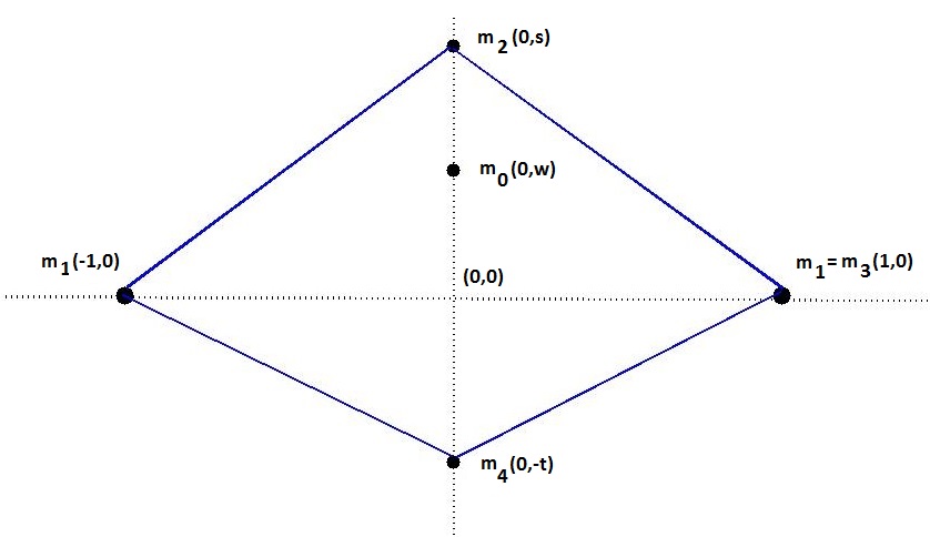
Fig. 1 : Rhomboidal five-body configurations.

Fig. 2 : Triangular five-body configurations.

Theorem 2

Consider two pairs of equal masses on the vertices of a rhombus with a fifth mass on one of the axis of symmetry. The five positive masses have their position vectors $\mathbf{r}_{0}=(0,w),$ $\mathbf{r}_{1}=(-1,0),$ $\mathbf{r}_{2}=(0,t),$ $\mathbf{r}_{3}=(1,0),$ $\mathbf{r}_{4}=(0,-t)$, where $t\in\mathbb{R}^{+},w\in\mathbb{R}\backslash\{0\}$. Then their is no central configuration of this type.

Theorem 3

Let $\mathbf{r}_{1}=(-1,0),$ $\mathbf{r}_{2}=(0,s),$ $\mathbf{r}_{3}=(1,0),$ $\mathbf{r}_{4}=(0,-t)$, where $s,t\in\mathbb{R}^{+}$. Then, the configuration $\mathbf{r}=(\mathbf{r}_{1},\mathbf{r}_{2},\mathbf{r}_{3},\mathbf{r}_{4})$ given in figure 1 will form a central configuration in the region

$$R_{\mu_{2}\mu_{4}}(s,t) = \{(s,t)|(0.268<t\leq 0.577\wedge$$ (20)

$$\wedge \frac{1-t^{2}}{2t}<s<\sqrt{3})\vee(0.577<t<\sqrt{3}\wedge$$

$$\wedge \sqrt{t^{2}+1}-t<s<\sqrt{3})\}.$$

Theorem 4

Let $\mathbf{r}_{0}=(0,w),$ $\mathbf{r}_{1}=(-1,0),$ $\mathbf{r}_{2}=(0,s),$ $\mathbf{r}_{3}=(1,0),$ $\mathbf{r}_{4}=(0,-t)$, where $s,t,w\in\mathbb{R}$.

1. The configuration $\mathbf{r}=(\mathbf{r}_{0},\mathbf{r}_{1},\mathbf{r}_{2},\mathbf{r}_{3},\mathbf{r}_{4})$ will form a central configuration with

   $$\mu_{0} = \frac{m_{0}}{m_{1}}=\frac{{A}_{{1}}{C}_{{2}}{C}_{{3}}-({B}_{{1}}{B}_{{3}}{C}_{{2}}+{B}_{{2}}{C}_{{1}}{C}_{{3}})}{{A}_{{2}}{C}_{{1}}{C}_{{3}}+{A}_{{3}}{B}_{{1}}{C}_{{2}}},$$

   $$\mu_{2} = \frac{m_{2}}{m_{1}}=\frac{{A}_{{3}}{B}_{{2}}{C}_{{1}}-({A}_{{1}}{A}_{{3}}{C}_{{2}}+{A}_{{2}}{B}_{{3}}{C}_{{1}})}{{A}_{{2}}{C}_{{1}}{C}_{{3}}+{A}_{{3}}{B}_{{1}}{C}_{{2}}},{}$$ (21)

   $$\mu_{4} = \frac{m_{4}}{m_{1}}=\frac{{A}_{{2}}{B}_{{1}}{B}_{{3}}-({A}_{{1}}{A}_{{2}}{C}_{{3}}+{A}_{{3}}{B}_{{1}}{B}_{{2}})}{{A}_{{2}}{C}_{{1}}{C}_{{3}}+{A}_{{3}}{B}_{{1}}{C}_{{2}}},$$

   where

   $$A_{1} = (R_{03}-R_{13})\Delta_{013},\quad A_{2}=(R_{10}-R_{20})\Delta_{120},$$

   $$A_{3} = (R_{10}-R_{40})\Delta_{140},$$

   $$B_{1} = (R_{02}-R_{12})\Delta_{012},\quad B_{2}=(R_{13}-R_{23})\Delta_{123},$$

   $$B_{3} = (R_{13}-R_{43})\Delta_{143},$$

   $$C_{1} = (R_{04}-R_{14})\Delta_{014},\quad C_{2}=(R_{14}-R_{24})\Delta_{124},$$

   $$C_{3} = (R_{12}-R_{42})\Delta_{142}.$$

2. The mass ratios $\mu_{0}>0$, $\mu_{2}>0$ and $\mu_{4}>0$ form a central configuration in

   $$R(t,w)=R_{\mu_{0}}\cap R_{\mu_{2}}\cap R_{\mu_{4}},$$ (22)

   where $R_{\mu_{0}}$, $R_{\mu_{2}}$ and $R_{\mu_{4}}$ are respectively given by equations (35), (39), and (41).

3 Proof of Theorem 2

In order to prove Theorem 2, we write Dziobek’s equations of Lemma 1 in a matrix form, after we substitute $m_{2}=m_{4}$:

$\displaystyle\hskip 0.0pt{\left[\begin{array}[]{ccc}0&B_{0}&C_{0}\\ A_{1}&B_{1}&C_{1}\\ A_{2}&-B_{1}&-C_{1}\end{array}\right]\cdot\left[\begin{array}[]{c}m_{0}\\ m_{1}\\ m_{2}\end{array}\right]=\left[\begin{array}[]{c}0\\ 0\\ 0\end{array}\right],}$

where

$$B_{0} = (R_{03}-R_{13})\Delta_{013},B_{1}=(R_{13}-R_{23})\Delta_{123},$$

$$A_{1} = (R_{10}-R_{20})\Delta_{120},A_{2}=(R_{10}-R_{40})\Delta_{140},$$

$$C_{1} = (R_{14}-R_{24})\Delta_{124},$$

$$C_{0} = (R_{02}-R_{12})\Delta_{012}+(R_{04}-R_{14})\Delta_{014}.$$

For the above system of equation, in order to have a non-trivial solution, the determinant of the augmented matrix must be zero. After adding row 2 with row 3 of the augmented matrix, the third row reduces to $\{A_{1}+A_{2},0,0\}$. Hence, $f_{A_{1}A_{2}}=A_{1}+A_{2}=0$ will imply the existence of non-trivial solution (the case $m_{0}=0$ will be discussed in detail in section 4). Therefore, from the remaining two equations

$$\mu_{1}=\frac{m_{1}}{m_{2}}=-\frac{C_{0}}{B_{0}},\text{ and \ }\mu_{0}=\frac{m_{0}}{m_{2}}=\frac{C_{1}B_{0}-C_{0}B_{1}}{B_{0}A_{2}}$$ (23)

we obtain that they will form a central configuration with respect to the geometric constraint

$$f_{A_{1}A_{2}} = (R_{01}-R_{02})\Delta_{012}+(R_{01}-R_{04})\Delta_{014}$$ (24)

$$= \frac{t-w}{|t-w|^{3}}-\frac{t+w}{|t+w|^{3}}+\frac{2w}{(w^{2}+1)^{\frac{3}{2}}}=0.$$

For positive solutions we must have $f_{A_{1}A_{2}}=0$ and $\mu_{1}>0$, $\mu_{2}>0$.

1. If $t>|w|,w\in\mathbb{R}\backslash\{0\}$ then $f_{A_{1}A_{2}}=0$ can be written as a polynomial in two variables $t$ and $w$ such that $t\neq\pm w$.

   $$G_{1}(w) := 2t^{4}w-4t^{2}w^{3}+4tw(w^{2}+1)^{3/2}+$$ (25)

   $$+ 2w^{5}=0.$$

   The polynomial $G_{1}(w)$ has two real negative roots and two complex roots. As we require $t>0$, therefore this case is not interesting.

   

   

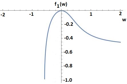
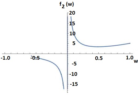
   Fig. 3 : a) $f_{1}(w)$                           b) $f_{2}(w)$

2. If $t<w,w>0$  then $f_{A_{1}A_{2}}=0$ can be written as a polynomial in two variables $t$ and $w$ such that $t\neq\pm w\neq 0$.

   $$G_{2}(w) := t^{4}w-t^{2}(2w^{3}+(1+{w^{2}})^{3/2})+$$ (26)

   $$+ w^{2}(w^{3}-(1+{w^{2}})^{3/2})=0.$$

   The polynomial $G_{2}(w)$ is quadratic in $t^{2}$ and will have four roots as functions of $w$.

3. $\displaystyle\hskip 0.0pt{t(w)=\pm\sqrt{\frac{(w^{2}+1)^{3/2}}{2w}+w^{2}\pm\frac{\sqrt{(w^{2}+1)^{3}+8w^{3}(w^{2}+1)^{3/2}}}{2w}}.}$

   The function

4. $\displaystyle\hskip 0.0pt{f_{1}(w)=\frac{(w^{2}+1)^{3/2}}{2w}+w^{2}-\frac{\sqrt{(w^{2}+1)^{3}+8w^{3}(w^{2}+1)^{3/2}}}{2w}}$

   is negative for all values of $w$, see figure 3a. The function

5. $\displaystyle\hskip 0.0pt{f_{2}(w)=\frac{(w^{2}+1)^{3/2}}{2w}+w^{2}+\frac{\sqrt{(w^{2}+1)^{3}+8w^{3}(w^{2}+1)^{3/2}}}{2w}}$

   is positive for $w>0$ (see figure 3b). Then $G_{2}(w)$ has two real roots with one positive and one negative root. The negative root is not interesting.

   The necessary condition for the existence of central configurations is satisfied at

6. $\displaystyle\hskip 0.0pt{t_{1}(w)=\sqrt{f_{2}(w)}.}$

   

   

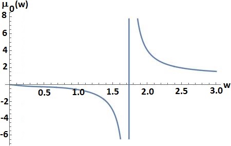
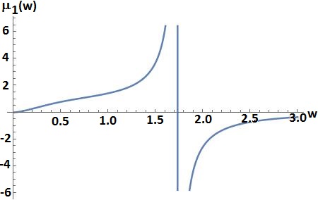
   Fig. 4 : a) $\mu_{0}(w)$ when $t=t_{1}(w)$      b) $\mu_{1}(w)$ when $t=t_{1}(w)$

   It is straightforward to see from figure 4 that $\mu_{0}(w)>0$ when $w<\sqrt{3}$, and $\mu_{1}(w)>0$ when $w>\sqrt{3}$. So, there is no common region where both $\mu_{0}(w)$ and $\mu_{1}(w)$ are positive (Fig. 5).

   

   

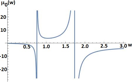
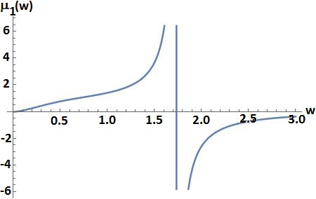
   Fig. 5 : a) $\mu_{0}(w)$ when $t=-t_{1}(w)$      b) $\mu_{1}(w)$ when $t=-t_{1}(w)$

7. If $t<|w|,w<0$ then $f_{A_{1}A_{2}}=0$ can be written as a polynomial in two variables $t$ and $w$ such that $t\neq\pm w\neq 0$.

   $$G_{3}(w) := t^{4}w+t^{2}((w^{2}+1)^{3/2}-2w^{3})+$$ (27)

   $$+ w^{2}(w^{3}+(w^{2}+1)^{3/2})=0.$$

The polynomial $G_{3}(w)$ is quadratic in $t^{2}$ and have the following four real roots as functions of $w$.

$$t_{2}(w)=-\sqrt{f_{3}(w)},\quad t_{3}(w)=\sqrt{f_{3}(w)},$$

$$t_{4}(w)=-\sqrt{f_{4}(w)},\quad t_{5}(w)=\sqrt{f_{4}(w)},$$

where

$\displaystyle\hskip 0.0pt{f_{3}(w)=-\frac{(w^{2}+1)^{3/2}}{2w}+w^{2}-\frac{\sqrt{(w^{2}+1)^{3/2}\cdot(1-8w^{3})}}{2w},}$

$\displaystyle\hskip 0.0pt{f_{4}(w)=-\frac{(w^{2}+1)^{3/2}}{2w}+w^{2}+\frac{\sqrt{(w^{2}+1)^{3/2}\cdot(1-8w^{3})}}{2w}.}$

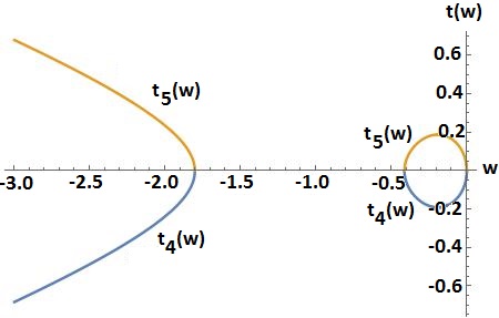
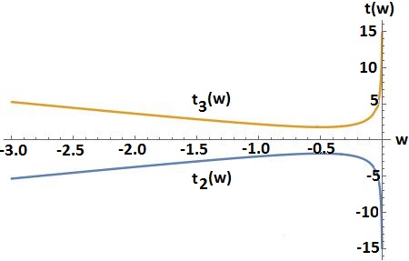
Fig. 6 : Roots of $G_{3}(w)$

Two of the above roots i.e. $t_{3}(w)$ and $t_{5}(w)$ are positive, and $t_{2}(w)$ and $t_{4}(w)$ are negative. These roots are given in figure 6.

By the close inspection of figure 6 it can be seen that $t_{3}(w)>|w|$ for all $w<0$. As a result, this root is invalid as we have the additional constraint of $t<|w|$ for this special case. The positive root $t_{5}(w)$ remains less than $|w|$ for $w<0$ when it is defined in $(-4,-1.8)$ and $(-0.4,0)$.

The mass ratio $\mu_{1}$ is positive when $w\in(-0.2,0)$ as $B_{0}$ and $C_{0}$ have opposite signs in this interval, see figure (7a). In the same interval $A_{2}B_{0}$ and $B_{0}C_{1}-B_{1}C_{0}$ have opposite signs and hence $\mu_{0}$ is negative, no central configurations at $t=t_{5}(w)$ when $w\in(-0.4,0)$. For $w<-1.8$, $C_{0}$ is an increasing function of $w$ with its absolute minimum, 0, occurring when $w\to-\infty$. Hence, $C_{0}>0$ for all $w<-1.8$. Similarly, $B_{0}$ is also positive. Therefore, $\mu_{1}<0$ for $w<-1.8$ (see figure 7b). This completes the proof of Theorem 2.

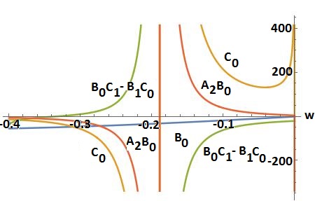
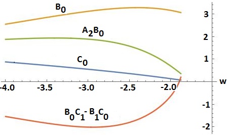
Fig. 7 : The curves $B_{0}$, $C_{0}$, $A_{2}B_{0}$ and $B_{0}C_{1}-B_{1}C_{0}$ at $t=t_{5}(w)$ such that a) $w\in(-0.4,0)$ b) $w\in(-4,-1.8)$.

4 Proof of Theorem 3

After substituting $m_{0}=0$ in the equations of Lemma 1 and using the resulting symmetries, the following reduced system of Dziobek’s equations is obtained:

$$(R_{13}-R_{23})\Delta_{123}m_{1}+(R_{14}-R_{24})\Delta_{124}m_{4} = 0,$$

$$(R_{13}-R_{14})\Delta_{134}m_{1}+(R_{12}-R_{24})\Delta_{124}m_{2} = 0,$$ (28)

where

$$R_{23} = (1+s^{2})^{-3/2},\quad R_{14}=(1+t^{2})^{-3/2},$$

$$R_{24} = (t+s)^{-3},$$

$$\Delta_{123} = -2s,\quad\Delta_{124}=-(s+t),\quad\Delta_{134}=-2t.$$

As the above system is under determined, therefore we define $\mu_{2}=m_{2}/m_{1}$ and $\mu_{4}=m_{4}/m_{1}$. Simultaneous solution of equations (28) gives

$$\mu_{2} = \frac{(s^{2}+1)^{3/2}t(s+t)^{2}f_{5}(t)}{4(t^{2}+1)^{3/2}f_{6}(s,t)},$$ (29)

$$\mu_{4} = \frac{sf_{7}(s)(t^{2}+1)^{3/2}(s+t)^{2}}{4(s^{2}+1)^{3/2}f_{8}(s,t)},$$ (30)

where

$$f_{5}(t) = ((t^{2}+1)^{3/2}-8),$$

$$f_{6}(s,t) = ((s^{2}+1)^{3/2}-(s+t)^{3}),$$

$$f_{7}(s) = ((s^{2}+1)^{3/2}-8),$$

$$f_{8}(s,t) = ((t^{2}+1)^{3/2}-(s+t)^{3}).$$

To find the central configuration (CC) regions, where all the masses are positive, we need to find regions in the $st$-plane, where both $\mu_{2}$ and $\mu_{4}$ are positive. As $f_{5}(t)$ is a monotonically increasing function of $t$ for all $t>0$, with a single zero at $t=\sqrt{3}$, therefore it is straightforward to see that $f_{5}(t)<0$, when $t<\sqrt{3}$. Solving $f_{6}(s,t)=0$ for variable $t$, we get $t(s)=-s+\sqrt{s^{2}+1}$. It is easy to check that $f_{6}(s,t)<0$ when $t(s)>-s+\sqrt{s^{2}+1}$. The two functions $f_{5}(t)$ and $f_{6}(s,t)$ are never simultaneously positive, therefore $\mu_{2}>0$ in

$$R_{\mu_{2}}=\{(s,t)|t>0\wedge s>0\wedge\sqrt{s^{2}+1}-s<t<\sqrt{3}\}.$$ (31)

Similarly, $f_{7}(s)=0$, when $s=\sqrt{3}$ and $f_{8}(s,t)=0$, when $s(t)=-t+\sqrt{t^{2}+1}$. Similar $\mu_{4}>0$ in

$$R_{\mu_{4}}=\{(s,t)|s>0\wedge t>0\wedge\sqrt{t^{2}+1}-t<s<\sqrt{3}\}.$$ (32)

The intersection of $R_{\mu_{2}}$ and $R_{\mu_{4}}$ is $R_{\mu_{2}\mu_{4}}$ given by the equation (20) (see Fig. 8).

Corollary 5

Consider $t<0$ in the setup of Theorem 3, guaranteeing a triangular four-body arrangement, then the configuration $(m_{1},m_{2},m_{1},m_{4})$ will form a triangular central configuration in

$$TR_{t_{-}}(s,t) = \{(s,t)|(-3.73<t<-\sqrt{3}\wedge$$

$$\wedge h_{1}(t)<s<\sqrt{3})\vee(-\sqrt{3}<t\leq-1\wedge$$

$$\wedge (0<s<h_{1}(t)\vee\sqrt{3}<s<h_{2}(t)))\vee$$

$$\vee (-1<t<-\frac{1}{\sqrt{3}}\wedge\sqrt{3}<s<h_{2}(t))$$

$$\vee (-\frac{1}{\sqrt{3}}<t<0\wedge h_{2}(t)<s<\sqrt{3})\},$$

where

$\displaystyle\hskip 0.0pt{h_{1}(t)=\frac{1-t^{2}}{2t},\quad h_{2}(t)=\sqrt{t^{2}+1}-t.}$

Proof. The proof of the Corollary 5 follows the same procedure as the Theorem 3. Therefore, we only give a sketch of this proof and leave the details to the interested readers.

Using the same procedure as above we can show that the mass $m_{2}$ is positive in the region

$$TR_{m_{2}}(s,t) = \{(s,t)|(0<s<\frac{1}{\sqrt{3}}\wedge(-\sqrt{3}<t<H(s)$$

$$\vee -s<t<0))\vee(\frac{1}{\sqrt{3}}<s<\sqrt{3}\wedge$$

$$\wedge (H(s)<t<-\sqrt{3}\vee-s<t<0))\vee$$

$$\vee (s>\sqrt{3}\wedge(H(s)<t<-s\vee$$

$$\vee -\sqrt{3}<t<0))\},$$

where

$\displaystyle\hskip 0.0pt{H(s)=-\sqrt{s^{2}+1}-s.}$

Similarly, $m_{4}$ is positive in the region

$$TR_{m_{4}}(s,t) = (t<-\sqrt{3}\wedge(0<s<\sqrt{3}\vee-t<s<h_{2}(t)))$$

$$\vee (-\sqrt{3}<t<-\frac{1}{\sqrt{3}}\wedge(0<s<-t\vee$$

$$\vee \sqrt{3}<s<h_{2}(t)))\vee(-\frac{1}{\sqrt{3}}<t<0\wedge$$

$$\wedge (0<s<-t\vee h_{2}(t)<s<\sqrt{3})).$$

The intersection of $TR_{m_{2}}(s,t)$ and $TR_{m_{4}}(s,t)$ give $TR_{t_{-}}(s,t).$   

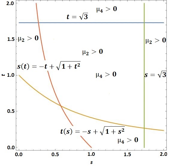
Fig. 8 : Central Configuration region in the case of Rhomboidal four-body problem

5 Proof of Theorem 4

5.1 Proof of Theorem 4a

Equations (12), (13) and (14) of Lemma 1 define the CC of rhomboidal or triangular five-body problems. Let $\mu_{0}=\frac{m_{0}}{m_{1}}$, $\mu_{2}=\frac{m_{2}}{m_{1}}$, $\mu_{4}=\frac{m_{4}}{m_{1}}$ and rewrite the equations from Lemma 1 as

$$A_{1}m_{1}+B_{1}m_{2}+C_{1}m_{4} = 0,$$

$$A_{2}m_{0}+B_{2}m_{1}+C_{2}m_{4} = 0,$$

$$A_{3}m_{0}+B_{3}m_{1}+C_{3}m_{2} = 0,$$

where

$$A_{1} = (R_{03}-R_{13})\Delta_{013},A_{2}=(R_{10}-R_{20})\Delta_{120},$$

$$A_{3} = (R_{10}-R_{40})\Delta_{140},$$

$$B_{1} = (R_{02}-R_{12})\Delta_{012},B_{2}=(R_{13}-R_{23})\Delta_{123},$$

$$B_{3} = (R_{13}-R_{43})\Delta_{143},$$

$$C_{1} = (R_{04}-R_{14})\Delta_{014},C_{2}=(R_{14}-R_{24})\Delta_{124},$$

$$C_{3} = (R_{12}-R_{42})\Delta_{142}.$$

Divide the above equations by $m_{1}$ and write them in the following matrix form:

$$\left[\begin{array}[]{ccc}0&B_{1}&C_{1}\\ A_{2}&0&C_{2}\\ A_{3}&C_{3}&0\end{array}\right]\cdot\left[\begin{array}[]{c}\mu_{0}\\ \mu_{2}\\ \mu_{4}\end{array}\right]=-\left[\begin{array}[]{c}A_{1}\\ B_{2}\\ B_{3}\end{array}\right].$$ (33)

After a number of row operation, a simultaneous solution of the above system is obtained as below.

$$\mu_{0} = \frac{{A}_{{1}}{C}_{{2}}{C}_{{3}}-({B}_{{1}}{B}_{{3}}{C}_{{2}}+{B}_{{2}}{C}_{{1}}{C}_{{3}})}{{A}_{{2}}{C}_{{1}}{C}_{{3}}+{A}_{{3}}{B}_{{1}}{C}_{{2}}},$$

$$\mu_{2} = \frac{{A}_{{3}}{B}_{{2}}{C}_{{1}}-({A}_{{1}}{A}_{{3}}{C}_{{2}}+{A}_{{2}}{B}_{{3}}{C}_{{1}})}{{A}_{{2}}{C}_{{1}}{C}_{{3}}+{A}_{{3}}{B}_{{1}}{C}_{{2}}},$$ (34)

$$\mu_{4} = \frac{{A}_{{2}}{B}_{{1}}{B}_{{3}}-({A}_{{1}}{A}_{{2}}{C}_{{3}}+{A}_{{3}}{B}_{{1}}{B}_{{2}})}{{A}_{{2}}{C}_{{1}}{C}_{{3}}+{A}_{{3}}{B}_{{1}}{C}_{{2}}}.$$

This completes the proof of Theorem 4a.

5.2 Proof of Theorem 4b

The required values of $R_{ij}$ and $\Delta_{ijk}$ can be generated from Lemma 1 by the substitution of $s=1$.

Lemma 6

The function

$\displaystyle\hskip 0.0pt{\mu_{0}=\frac{{A}_{{1}}{C}_{{2}}{C}_{{3}}-({B}_{{1}}{B}_{{3}}{C}_{{2}}+{B}_{{2}}{C}_{{1}}{C}_{{3}})}{{A}_{{2}}{C}_{{1}}{C}_{{3}}+{A}_{{3}}{B}_{{1}}{C}_{{2}}}}$

attains positive value in the region

$$R_{\mu_{0}}=(R_{D}\cap R_{N_{\mu_{0}}})\cup(R_{D}^{c}\cap R_{N_{\mu_{0}}}^{c}),$$ (35)

where $R_{D}^{c}$ and $R_{N_{\mu_{0}}}^{c}$ are the complements of the regions $R_{D}$ and $R_{N_{\mu_{0}}}$.

Proof. Let $N_{\mu_{0}}={A}_{{1}}{C}_{{2}}{C}_{{3}}-({B}_{{1}}{B}_{{3}}{C}_{{2}}+{B}_{{2}}{C}_{{1}}{C}_{{3}})$ and $D={A}_{{2}}{C}_{{1}}{C}_{{3}}+{A}_{{3}}{B}_{{1}}{C}_{{2}}.$ For $\mu_{0}$ to be positive, $N_{\mu_{0}}$ and $D$ must have the same sign.

The denominator $D$ will be positive when both factors ${A}_{{2}}{C}_{{1}}{C}_{{3}}$ and $A_{3}B_{1}C_{2}$ are positive or at least one of them is positive, such that the positive part is greater than the absolute value of the negative part. Both these factors are positive in

$$R_{da}(t,w) = \{(t,w)|(0<w\leq 0.41\wedge d_{1}(w)<t<1)$$ (36)

$$\vee (0.41<w<0.58\wedge d_{1}<t<0.5\cdot d_{2}(w))$$

$$\vee (w>2.41\wedge 0.41<t<1)\},$$

where

$\displaystyle\hskip 0.0pt{d_{1}(w)=\sqrt{w^{2}+1}-w,\quad d_{2}(w)=\frac{(1-w^{2})}{w}.}$

Similarly, when

1. ${A}_{{2}}{C}_{{1}}{C}_{{3}}>0$ and $A_{3}B_{1}C_{2}<0$ then ${A}_{{2}}{C}_{{1}}{C}_{{3}}$ $>$ $|A_{3}B_{1}C_{2}|$ in the following region.

   $$R_{db}(t,w) = \{(t,w)|(0.4<t\leq 0.58\wedge$$

   $$\wedge 0.6\cdot d_{2}(t)<w<1)\vee$$

   $$\vee (0.58<t<1\wedge d_{1}(t)<w<1)\}.$$

2. ${A}_{{2}}{C}_{{1}}{C}_{{3}}<0$ and $A_{3}B_{1}C_{2}>0$ then $A_{3}B_{1}C_{2}$ $>$ $|{A}_{{2}}{C}_{{1}}{C}_{{3}}|$ in the following region.

   $$R_{dc}(t,w) = \{(t,w)|(w\leq-1.49\wedge 0<t<0.23)$$

   $$\vee (-1.49<w<-1\wedge$$

   $$\wedge 0<t<0.2\cdot d_{2}(w))\vee$$

   $$\vee (1<w<2.41\wedge 0.41<t\leq 1)\}.$$

Therefore, the denominator $D$ is positive in (see Fig. 9a):

$$R_{D}=R_{da}(t,w)\cup R_{db}(t,w)\cup R_{dc}(t,w).$$ (37)

The numerator of $\mu_{0}$, $N_{\mu_{0}}$ is positive in (see Fig. 9b and Appendix):

$$R_{N_{\mu_{0}}}=R_{cN_{\mu_{0}}}(t,w)\cup R_{dN_{\mu_{0}}}(t,w).$$ (38)

Therefore, $\mu_{0}>0$ in the intersection of $R_{D}$ and $R_{N_{\mu_{0}}}$, and the intersection of their complements. Region $R_{\mu_{0}}$ is shown in figure 9c. This completes the proof of Lemma 6.

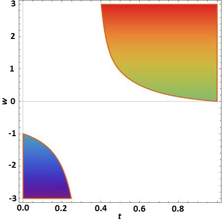
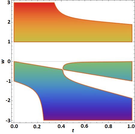
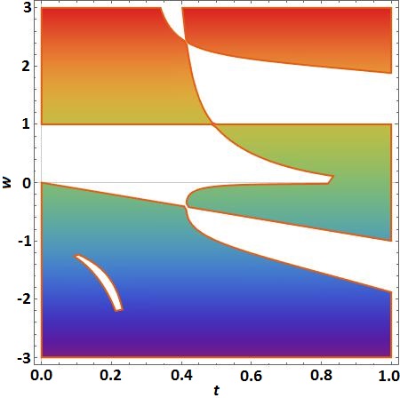
Fig. 9 : Regions a)$R_{D}$ (colored) b) $R_{N_{\mu_{0}}}$ (colored) c) $R_{\mu_{0}}$ (colored).

 

Lemma 7

The function

$\displaystyle\hskip 0.0pt{\mu_{2}=\frac{A_{3}B_{2}C_{1}-(A_{1}A_{3}C_{2}+A_{2}B_{3}C_{1})}{{A}_{{2}}{C}_{{1}}{C}_{{3}}+{A}_{{3}}{B}_{{1}}{C}_{{2}}}}$

attains positive values in the region

$$R_{\mu_{2}}=(R_{D}\cap R_{N_{\mu_{2}}})\cup(R_{D}^{c}\cap R_{N_{\mu_{2}}}^{c}),$$ (39)

where  $R_{D}^{c}$ and $R_{N_{\mu_{2}}}^{c}$ are complements of the regions $R_{D}$ and $R_{N_{\mu_{2}}}$ respectively.

Proof. Let $N_{\mu_{2}}=A_{3}B_{2}C_{1}-(A_{1}A_{3}C_{2}+A_{2}B_{3}C_{1}).$ For $\mu_{2}$ to be positive, $N_{\mu_{2}}$ and $D$ must have the same sign. We have given the complete analysis of $D$ in Lemma 6. Now, we need to find regions where $N_{\mu_{2}}$ is positive. It is proved in the appendix that $N_{\mu_{2}}(t,w)>0$ in

$$R_{N_{\mu_{2}}}=R_{aN_{\mu_{2}}}(t,w)\cup R_{bN_{\mu_{2}}}(t,w)\cup R_{cN_{\mu_{2}}}(t,w).$$ (40)

Region $R_{N_{\mu_{2}}}$ is shown in figure 10a. Consequently, $\mu_{2}>0$ in the intersection of $R_{D}$ and $R_{N_{\mu_{2}}}$, as well as the intersection of their complements. Region $R_{\mu_{2}}$ is shown in figure 10b. This completes the proof of Lemma 7.

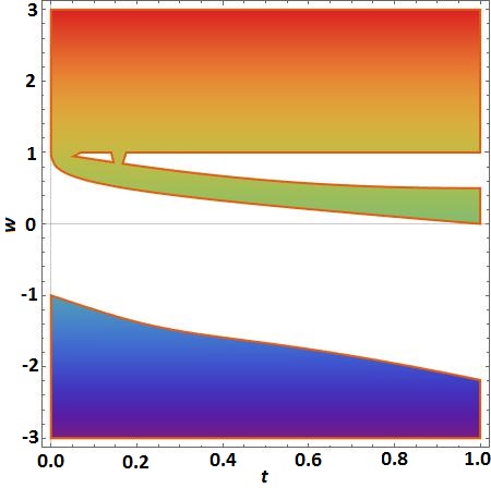
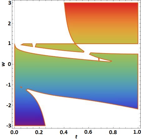
Fig. 10 : Regions a) $R_{N_{\mu_{2}}}$ (colored) b) $R_{\mu_{2}}$ (colored).

 

Lemma 8

The function

$\displaystyle\hskip 0.0pt{\mu_{4}=\frac{A_{2}B_{1}B_{3}-(A_{3}B_{1}B_{2}+A_{1}A_{2}C_{3})}{A_{2}C_{3}C_{1}+A_{3}B_{1}C_{2}}}$

attains positive values in the region

$$R_{\mu_{4}}=(R_{D}\cap R_{N_{\mu_{4}}})\cup(R_{D}^{c}\cap R_{N_{\mu_{4}}}^{c}).$$ (41)

Proof. Let $N_{\mu_{4}}=A_{2}B_{1}C_{3}-(A_{3}B_{1}B_{2}+A_{1}A_{2}C_{3}).$ For positive $\mu_{4}$, $N_{\mu 4}$ and $D$ must have the same sign. We have given the complete analysis of $D$ in Lemma 6. Now, we need to find regions where $N_{\mu_{4}}$ is positive. It is shown in the appendix that $N_{\mu_{4}}(t,w)$ is positive in (see Fig. 11a):

$$R_{N_{\mu_{4}}}=R_{aN_{\mu_{4}}}(t,w)\cup R_{bN_{\mu_{4}}}(t,w)\cup R_{cN_{\mu_{4}}}(t,w).$$ (42)

Thus, $\mu_{4}>0$ in the intersection of $R_{D}$ and $R_{N_{\mu_{4}}}$, as well as the intersection of their complements. Region $R_{\mu_{4}}$ is shown in figure 11b. This completes the proof of Lemma 8.   

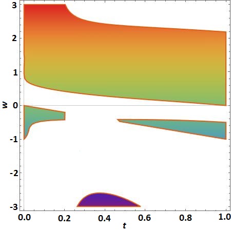
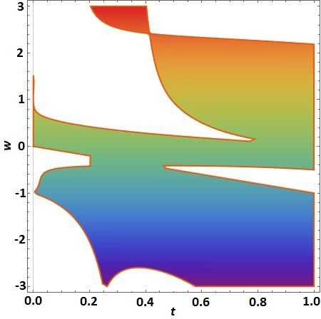
Fig. 11 : Regions a) $R_{N_{\mu_{4}}}$ (colored) b) $R_{\mu_{4}}$ (colored).

The central configuration region where all the masses have positive values is determined by

$$R(t,w)=R_{\mu_{0}}\cap R_{\mu_{2}}\cap R_{\mu_{4}}.$$ (43)

The region $R(t,w)$ is given in figure 12. This completes the proof of Theorem 4b. To better understand the nature of the complicated CC regions in figure 12, a number of relevant examples are given in figures 13 and 14.

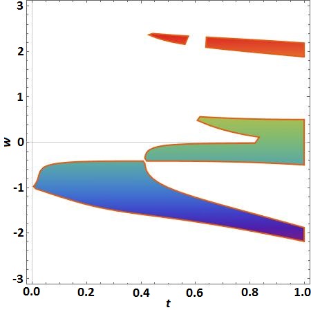
Fig. 12 : Region ($R(t,w)$) of central configuration in the case of Rhomboidal 5-body problem.

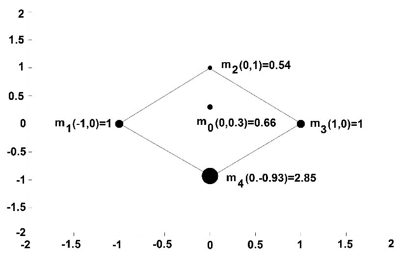
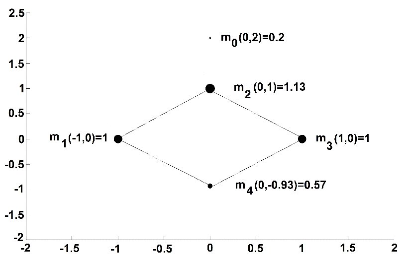
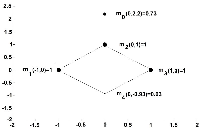
Fig. 13 : Three examples of rhomboidal five-body CC when $w>0$

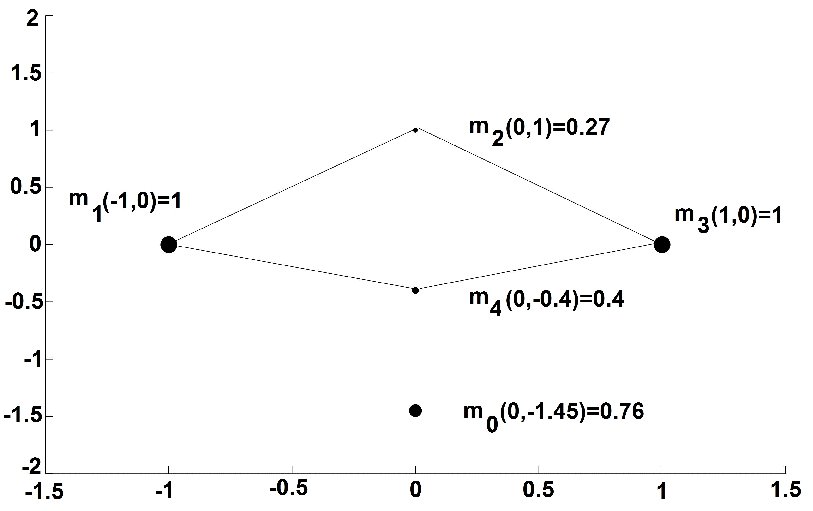
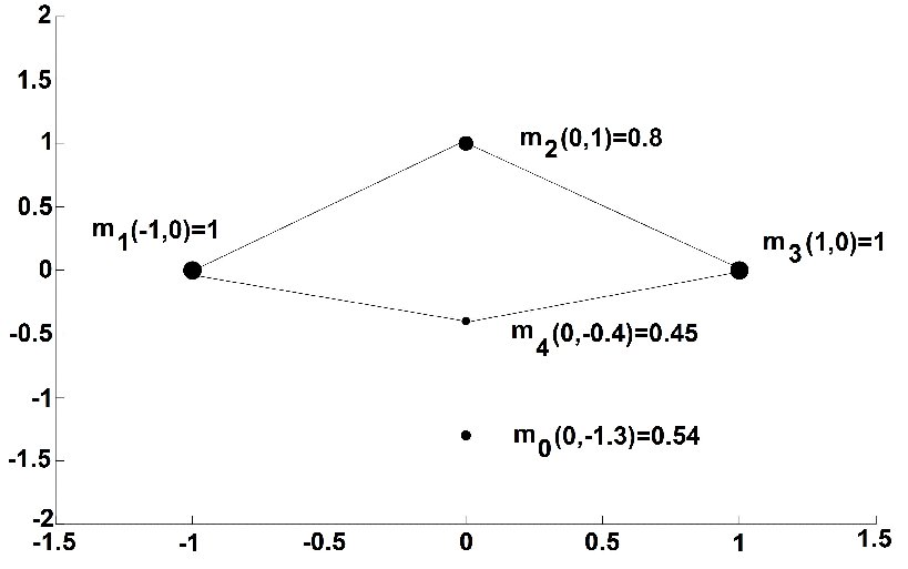
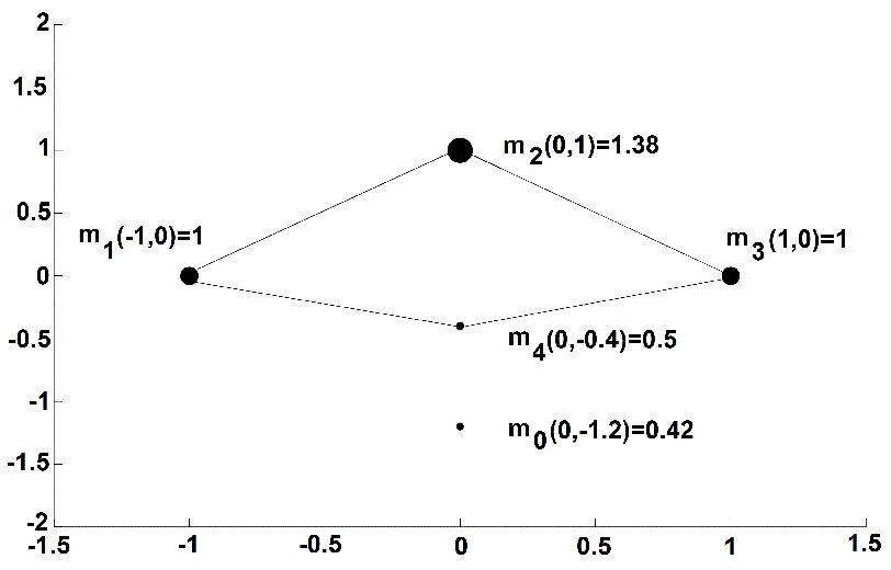
Fig. 14 : Three examples of rhomboidal five-body CC when $w<0$

The considered variables $t\in(-1,0)$ and $s=1$ in Lemma 1, will give the five-body triangular configurations shown in figure 2.

Corollary 9

Consider $t\in(-1,0)$ in the setup of Theorem 4, guaranteeing a triangular five-body arrangement for $w>0$. Then the configuration $(m_{0}$, $m_{1}$, $m_{2}$, $m_{1}$, $m_{4})$ will form a central configuration in region:

$$R_{t_{-}}(t,w)=R_{m_{0}}(t,w)\cap R_{m_{2}}(t,w)\cap R_{m_{4}}(t,w).$$ (44)

Proof. Consider $t<0$ and solve the equation (33) in the same way as in the proof of Theorem 4 to obtain the following regions of central configurations for the isosceles triangular five-body problem, given in figure 2. We will give a sketch of the proof, and details to the interested readers (as it follows the same procedure as in Theorem 4). The denominator is always negative when $w>0$. Therefore, the mass ratios $\mu_{0}$, $\mu_{2}$ and $\mu_{4}$ will be positive when their respective numerators are negative. Thus, the central configuration regions where $\mu_{0}$, $\mu_{2}$ and $\mu_{4}$ are respectively positive, are given below.

$$R_{m_{0}} = (-1<t<-w\wedge 0<w<1)\vee$$

$$\vee (1<w<1.73\wedge(-1<t<d_{2}(w)\vee$$

$$\vee \frac{0.5}{w}-0.5w<t<0))\vee 1.5<w<p),$$

$$R_{m_{2}} = (0<w<1\wedge(-1<t<-w\vee-w<t<0))$$

$$\vee (-1<t<d_{2}(w)\wedge 1.73205<w<2.41421)$$

$$\vee t>d_{2}(w),$$

$$R_{m_{4}} = (0<w<1\wedge-w<t<0)\vee$$

$$\vee (1<w<1.73205\wedge-1<t<0)\vee$$

$$\vee (1.73<w<q)\vee(1.6<w<r),$$

where

$$p(t) = 84.13t^{5}+301.01t^{4}+424.28t^{3}+295.98t^{2}+$$

$$+ 103.56t+16.68,$$

$$q(t) = -3.91t^{3}-7.57t^{2}-4.22t+1.22,$$

$$r(t) = 305.66t^{3}+52t^{2}+0.25t+1.76.$$

The central configuration region for the triangular five-body problem is

$$R_{t_{-}}(t,w)=R_{m_{0}}(t,w)\cap R_{m_{2}}(t,w)\cap R_{m_{4}}(t,w).$$ (45)

This region is given in figure 15d alongside $R_{m_{0}}$ (figure 15a)$,R_{m_{2}}($figure 15b) and $R_{m_{4}}$(figure 15c). The CC region in the figure 15 corresponds to the triangular solutions of the five-body problem.

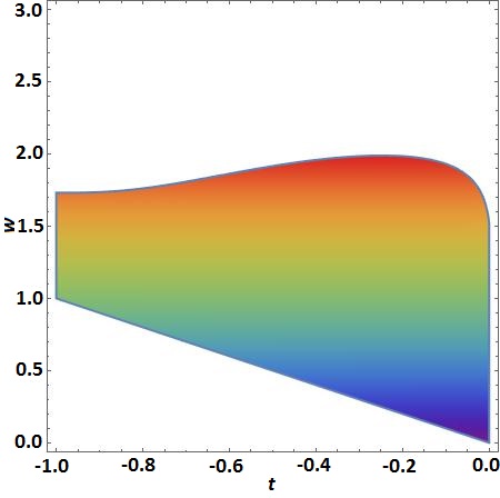
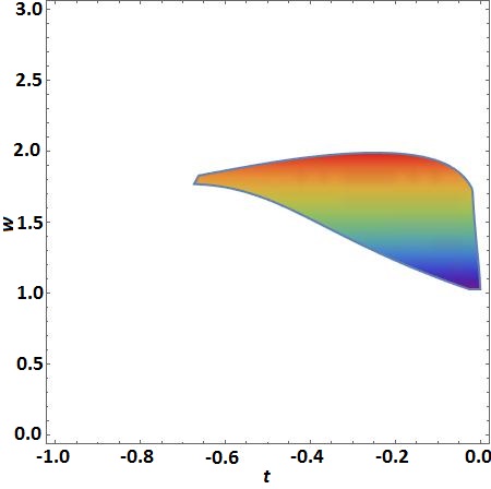
Fig. 15 : Regions of central configuration in the case of triangular five-body problem a) $m_{0}>0$, $R_{m_{0}}(t,w)$ b) $m_{2}>0$, $R_{m_{2}}(t,w)$ c) $m_{4}>0$, $R_{m_{4}}(t,w)$ d) $m_{i}>0$, $i=0,2,4$, $R_{t_{-}}(t,w)$.

 

Similarly, by taking $s=\sqrt{3}$, the configuration in figure 2 will become an equilateral triangle. The CC regions for this equilateral triangle five-body configuration can be found in the same way as in Theorem 4 or Corollary 9. Figure 16 shows the physical position of masses in the case of triangular five-body central configurations.

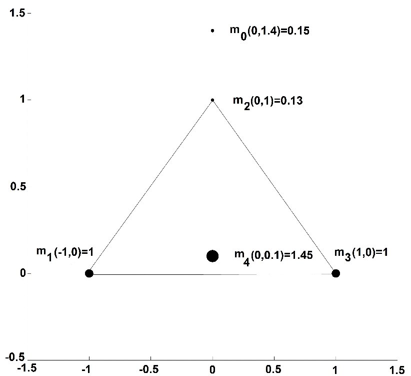
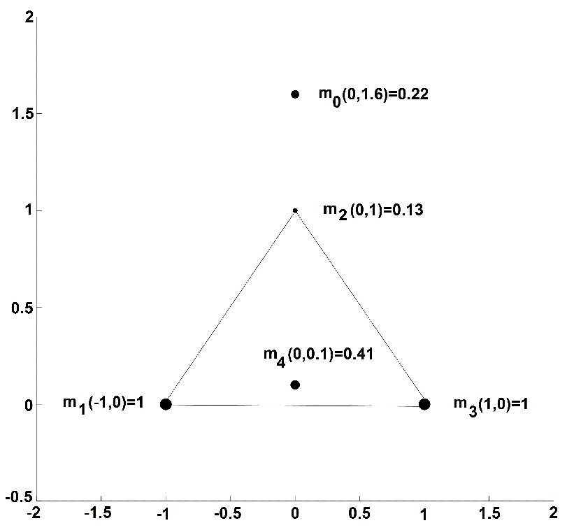
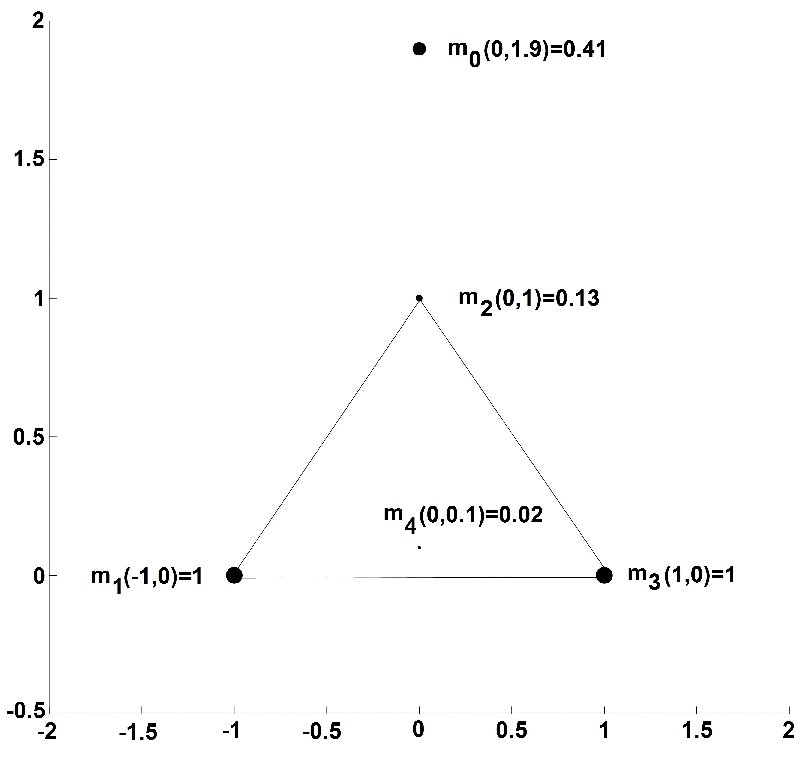
Fig. 16 : Three examples of triangular five-body CC

Note:

It is impossible to find analytically the CC regions in the full general cases, i.e. without fixing $s=1$. However, in the current analysis, the majority of the solutions are obtained.

6 Hamiltonian formulation and numerical applications

In this section, we will introduce the Hamiltonian formalism for the rhomboidal five-body problem. This five-body problem is introduced in Lemma 1. Then we are going to use regularized equations and Poincaré surface of section to investigate the effect of the increasing value of central mass on the stability of the proposed five-body problem. Using Poincaré surface of section we will study two special cases to identify chaotic regions and quasi-periodic orbits, with a special focus on the varying central mass. The two cases are:

1. Four equal masses with a varying central mass.

2. Two pairs of equal masses at the vertices of the rhombus with a varying central mass.

Two particular cases with only two degrees of freedom are known for the four-body problem, namely the one-dimensional symmetric four-body problem and the rhomboidal symmetric four-body problem (see Lacomba & Perez-Chavela (1993)). These two problems are simpler, but they still have chaotic solutions. As Diacu (2003) showed, symmetries played an essential role in searching for periodic orbits in most of the problems of celestial mechanics (Mioc & Barbosu, 2003). The Hamiltonian system in two degrees of freedom can be conveniently investigated using the Poincaré surface of section. The Poincaré section plays an important role in understanding the few-body problem, specifically the existence of periodic orbits (Burgos-Garcia & Delgado, 2013).
Let us consider five point masses $m_{1}(x_{1}=-x_{3},0)$, $m_{2}(0,y_{2})$, $m_{3}(x_{3},0)$, $m_{4}(0,-y_{4})$, and $m_{5}(0,y_{5})$ in a fixed plane $Oxy$ (see Fig. 1). Let us take $m_{1}=m_{3}$, and the generalized momenta as $p_{i}^{\prime}$, where $i=\overline{1,n}$, to get the Hamiltonian:

$$H = \sum_{i=1}^{5}\frac{{p^{\prime}}_{i}^{2}}{m_{i}}-\frac{2m_{1}m_{2}}{\sqrt{x_{3}^{2}+{y_{2}}^{2}}}-\frac{2m_{1}m_{4}}{\sqrt{x_{3}^{2}+{y_{4}}^{2}}}-\frac{2m_{1}m_{5}}{\sqrt{x_{3}^{2}+{y_{5}}^{2}}}-$$ (46)

$$- \frac{m_{1}^{2}}{2x_{3}}-\frac{m_{2}m_{4}}{\sqrt{(y_{4}+y_{2})^{2}}}-\frac{m_{2}m_{5}}{\sqrt{(y_{5}-y_{2})^{2}}}-\frac{m_{4}m_{5}}{\sqrt{(y_{4}+y_{5})^{2}}}.$$

Consider $m_{2}=m_{4}$ to be symmetric on the axis $Oy$, ($y_{2}=y_{4}$), and the mass $m_{5}=m_{0}$ stationary at the origin ($y_{5}=0$). The Hamiltonian then becomes:

$$H = \frac{{p^{\prime}}_{2}^{2}}{2m_{2}}+\frac{{p^{\prime}}_{3}^{2}}{2m_{1}}-\frac{2m_{1}m_{2}}{\sqrt{x_{3}^{2}+{y_{2}}^{2}}}-$$ (47)

$$- \frac{m_{1}(m_{1}+4m_{0})}{4x_{3}}-\frac{m_{2}(m_{2}+4m_{0})}{4y_{2}}.$$

Represent the generalized coordinates as $x_{3}:=q_{1}$, and $y_{2}:=q_{2}$, and the generalized momenta as $p_{3}^{\prime}:=p_{1}$, and $p_{4}^{\prime}:=p_{2}$, then the corresponding Hamiltonian takes the form

$$H = \frac{p_{1}^{2}}{2m_{1}}+\frac{p_{2}^{2}}{2m_{2}}-\frac{2m_{1}m_{2}}{\sqrt{q_{1}^{2}+{q_{2}}^{2}}}-$$ (48)

$$- \frac{m_{1}(m_{1}+4m_{0})}{4q_{1}}-\frac{m_{2}(m_{2}+4m_{0})}{4q_{2}},$$

The corresponding canonical equations of motion are

$$q_{1} = \frac{p_{1}}{m_{1}},$$ (49)

$$q_{2} = \frac{p_{2}}{m_{2}},$$

$$p_{1} = -\frac{2m_{1}m_{2}}{(q_{1}^{2}+{q_{2}}^{2})^{3/2}}q_{1}-\frac{m_{1}(m_{1}+4m_{0})}{2q_{1}^{2}},$$

$$p_{2} = -\frac{2m_{1}m_{2}}{(q_{1}^{2}+{q_{2}}^{2})^{3/2}}q_{2}-\frac{m_{2}(m_{2}+4m_{0})}{2q_{2}^{2}}.$$

Since we have singularities in the equations of motion, we use a regularization technique, called the double Levi-Civita transformation to regularize the Hamiltonian (see Szücs-Csillik (2016)).

Introduce the fictitious time $\tau$ as

$$\frac{dt}{d\tau}=q_{1}q_{2},$$ (50)

and the transformed coordinates as

$$q_{i}=Q_{i}^{2},i=1,2.$$ (51)

In order to achieve regularization we extend the coordinate transformation to a canonical transformation by introducing the generating function $W$ (see Csillik (2003)) as

$$W=p_{1}Q_{1}^{2}+p_{2}Q_{2}^{2}.$$ (52)

From the generating function $P_{j}=\sum\limits_{i=1}^{2}p_{i}\frac{\partial q_{i}}{\partial Q_{j}}$, $j=1,2$, we obtain the transformed momenta

$$p_{i}=\frac{P_{i}}{2Q_{i}},i=1,2,$$ (53)

where $P_{i}$ are the new momenta.

The canonical symplectic form of equations (49) will be preserved, if the new Hamiltonian is

$$\overline{H}=H-h_{0},$$ (54)

where $h_{0}$ is the constant of total energy.

Therefore, the transformed Hamiltonian is given by

$$\overline{H} = \frac{1}{8}\left(\frac{P_{1}^{2}Q_{2}^{2}}{m_{1}}+\frac{P_{2}^{2}Q_{1}^{2}}{m_{2}}\right)-\frac{1}{4}(m_{1}(4m_{0}+m_{1})Q_{2}^{2}$$

$$+ m_{2}(4m_{0}+m_{2})Q_{1}^{2})-\frac{2m_{1}m_{2}Q_{1}^{2}Q_{2}^{2}}{\sqrt{Q_{1}^{4}+Q_{2}^{4}}}-h_{0}Q_{1}^{2}Q_{2}^{2},$$

and the transformed equations of motion are

$$\frac{dQ_{i}}{d\tau} = \frac{\partial\overline{H}}{\partial P_{i}},$$ (55)

$$\frac{dP_{i}}{d\tau} = -\frac{\partial\overline{H}}{\partial Q_{i}},\quad i=1,2.$$

To construct the Poincaré surface of section and find the corresponding periodic orbits (see Cheb-Terrab & Oliveira (1996)), we plot the motion from the 4D phase space ($Q_{1}$, $Q_{2}$, $P_{1}$, $P_{2}$) in a ”cut” plane ($Q_{1}=0$, $Q_{2}$, $P_{1}>0$, $P_{2}$). Since $\overline{H}$ is conserved, any point in this surface of section will uniquely define the orbit.

To investigate the effect of central mass on the existence of quasi-periodic orbits, consider $m_{1}=m_{2}=$$m_{3}=$$m_{4}=1$ and

• $m_{0}=1$,

• $m_{0}=3$,

• $m_{0}=5$.

Consider $Q_{1}(0)=0$ and $P_{1}(0)>0$, to investigate the motion in the $(Q_{2},P_{2})$ plane, where the corresponding constant total energy $h_{0}$ have the values $-0.46$, $-0.9,$ and $-1.3$. Figures 17, 18, and 19 show the results for the gradually increased central mass. In addition, we also give a representative periodic orbit in each case.

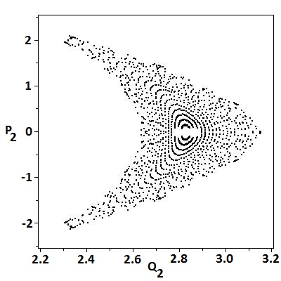
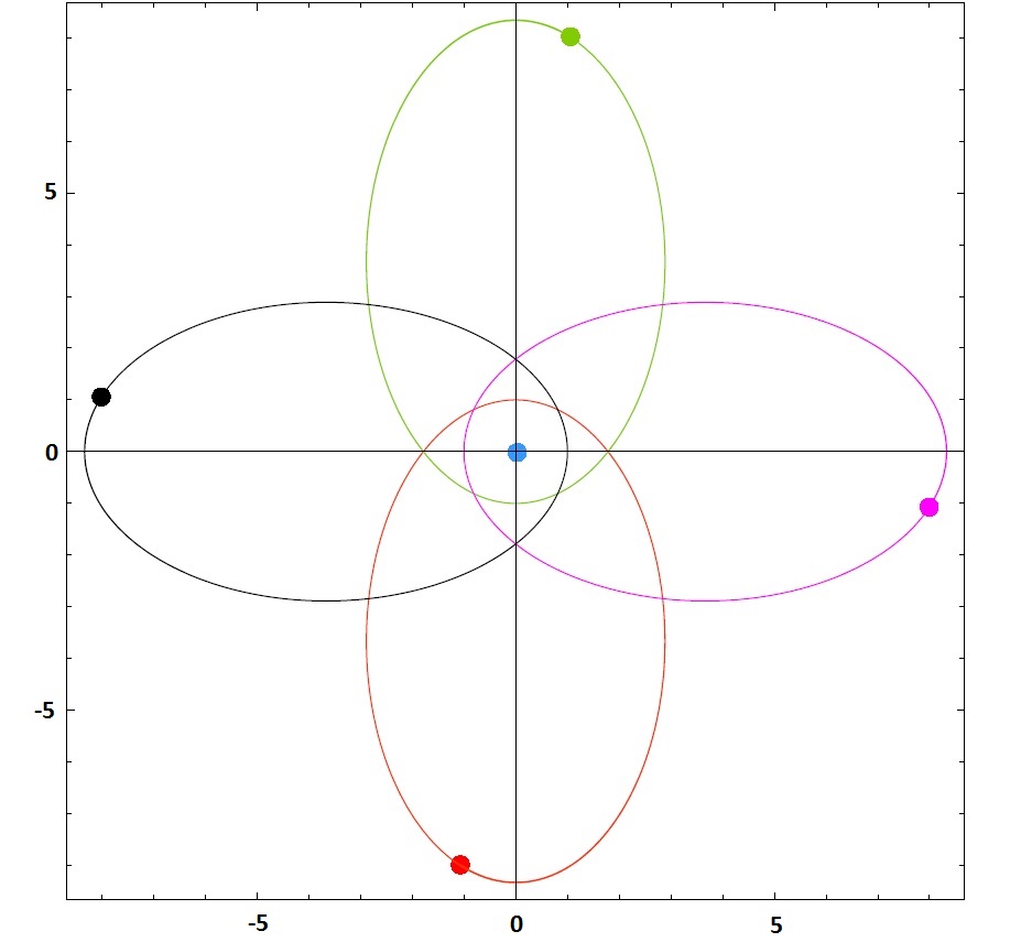
Fig. 17 : a) Poincaré section, when the central mass is $1$. b) A representative periodic orbit corresponding to the centre.

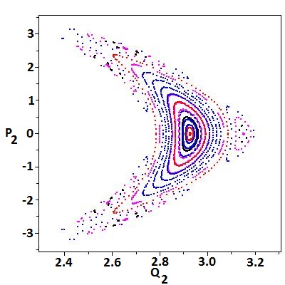
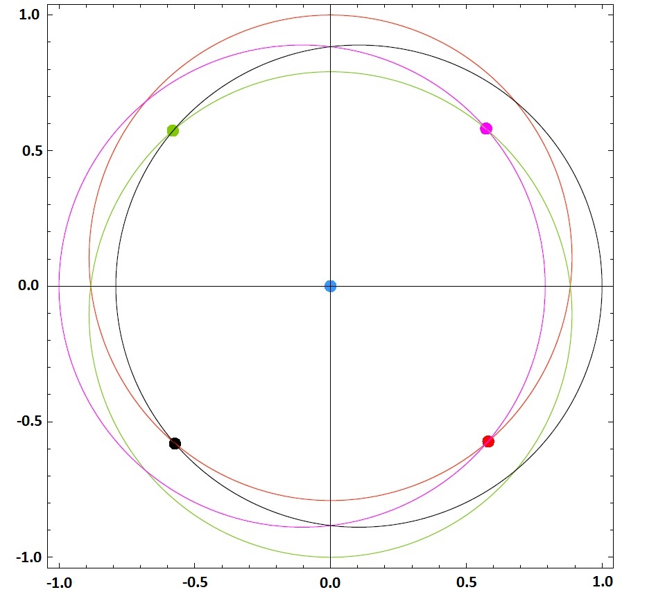
Fig. 18 : Poincaré section, when the central mass is $3$. b) A representative periodic orbit corresponding to the centre

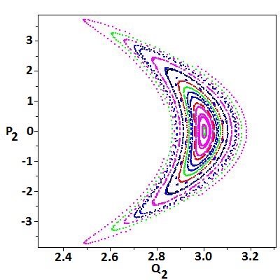
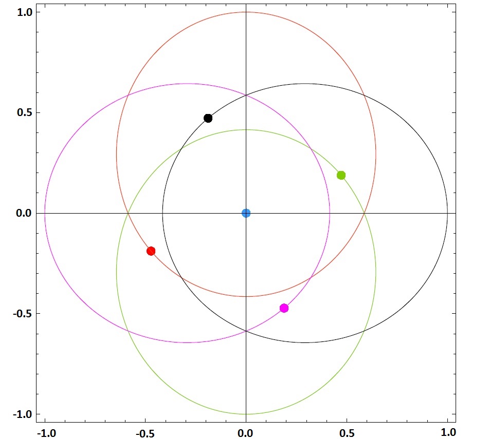
Fig. 19 : a) Poincaré section, when the central mass is $5$. b) A representative periodic orbit corresponding to the centre.

In the equal mass case, there are a couple of quasi-periodic orbits at and around $P_{2}=0$ and $Q_{2}=2.83$ (Fig. 17). The rest of the points in figure 17 are indicative of chaotic behavior. In figure 18, the central mass is increased to $m_{0}=3$. It is clear from figure 18 that the region with periodic orbits has begun to increase in size. Although the outer region is still chaotic but in inner region appears some regular structures. This is indicative of some underlying structure in the dynamics. At $m_{0}=5$, five times bigger than the outer masses, we can see higher number of quasi-periodic orbits around $Q_{2}=3$. The chaotic behavior which was very clear in the equal mass case has completely disappeared. This indicates that the increase in central mass plays a stabilizing role. Similar behavior was reported by Shoaib et al. (2008) for the hierarchical stability of the Caledonian symmetric five-body problem (CS5BP).

To complete the analysis given above, we discuss two more examples with two pairs of equal masses at the vertices of the rhombus, and other example with one pairs of equal masses on the $x-$axis and three different masses on the $y-$axis (see Fig. 13, 14 and 16). Consider

• $m_{1}=1$, $m_{2}=2$, and the central mass $m_{0}=0.05$ ($h_{0}=-0.9$);

• $m_{1}=1$, $m_{2}=1.1$, and the central mass $m_{0}=3$ ($h_{0}=-0.9$).

• $m_{1}=m_{3}=1$, $m_{2}=0.27$, $m_{4}=0.4$, $m_{0}=0.76$ ($h_{0}=-0.9$).

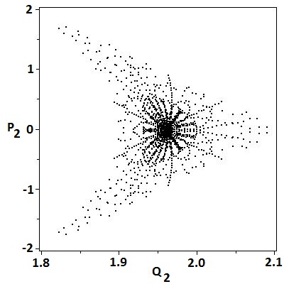
Fig. 20 : Poincaré section in case a.

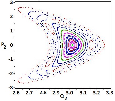
Fig. 21 : Cross section at $Q_{1}=0$ in case b., showing the quasi-periodic orbits.

As in case a., the surfaces in figures 20 and 21 show various types of orbits, including both circle-like quasi-periodic orbits and island orbits. Note the deformation in some of the circular orbits, indicating the presence of nearby island orbits. When the central body is small, the surface of section presents very few quasi-periodic orbits surrounded by chaotic region. As before, the increase in central mass completely changes the dynamics of the problem. A direct comparison of figures 17 with figures 21 reveal the obvious effect of changing central mass on the stability and existence of quasi-periodic orbits in the rhomboidal five-body problem introduced in section 1.

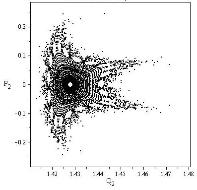
Fig. 22 : Poincaré section in case c.

In case c. (see Fig. 14a) three non-equal masses are distributed on the $y-$axis. We used the general form of the Hamiltonian (equation 46), and the notations: $x_{3}:=q_{1}$, $y_{2}:=q_{2}$, $m_{5}$=$m_{0}$. $y_{4}$ and $y_{5}$ are functions of $q_{2}$. As in previous cases, we constructed the corresponding new Hamiltonian (this transformation is trivial) and took $y_{4}=q_{2}-1.4$ and $y_{5}=q_{2}-2.45$. In this case we obtain the Poincaré surface of section shown in figure 22. The inner region of figure 22 points to the existence of regular structure and some quasi periodic orbits. The outer region exhibits chaotic behaviour.

7 Conclusions

In this paper we studied the central configurations of rhomboidal and triangular four- and five-body problems. (The configuration has only one symmetry with $m_{1}=m_{3}\neq m_{2}\neq m_{4}\neq m_{0}$). First, Dziobek’s equations are derived for this particular set up. Then, we derive regions of central configuration for various special cases of the general problem. We prove that no central configurations are possible when two pairs of masses are placed at the vertices of a rhombus, (which is symmetric both about the $x-$axis and the $y-$axis) and the fifth mass is placed anywhere on the axis of symmetry, except the origin. Using analytical techniques, regions of central configurations are derived for all other cases, including rhomboidal four- and five-body problems, isosceles and equilateral triangular five-body problems. To complement the analytical results, these regions are also explored numerically. Equations of motion are regularized using the double Levi-Civita transformations, and from the regularized equations we identify regions with quasi-periodic orbits. Moreover, we investigate the chaotic behavior in the phase space by means of the Poincaré sections. We show that if we increase the central mass, this has a stabilizing effect on the rhomboidal five-body configuration.

Appendix

Derivation of $R_{N_{\mu_{0}}}$:

The numerator of $\mu_{0}$, $N_{\mu_{0}}$ is positive when ${A}_{{1}}{C}_{{2}}{C}_{{3}}$ $>0$ and ${B}_{{1}}{B}_{{3}}{C}_{{2}}+{B}_{{2}}{C}_{{1}}{C}_{{3}}<0$ or when both factors have opposite sign and the positive factor is greater than the absolute value of the negative factor. All these possibilities are listed below with the corresponding regions, where $N_{\mu_{0}}>0$

1. ${A}_{{1}}{C}_{{2}}{C}_{{3}}>0$ and ${B}_{{1}}{B}_{{3}}{C}_{{2}}+{B}_{{2}}{C}_{{1}}{C}_{{3}}<0$: Using numerical approximation techniques it is obtained that $N_{\mu_{0}}>0$ in the following region:

   $$R_{cN_{\mu_{0}}}(t,w)=R_{aN_{\mu_{0}}}(t,w)\cup R_{bN_{\mu_{0}}}(t,w),$$ (56)

   where

   $$R_{aN_{\mu_{0}}}(t,w) = \{(t,w)|(0<t<0.41\wedge 0<w<1)$$

   $$\vee (0.41<t<1\wedge w>2.41)\vee(-1.73$$

   $$< w\leq-1.5\wedge 0.75\cdot d_{2}(w)<t<1)\},$$

   $$R_{bN_{\mu_{0}}}(t,w) = (w<-1.8\wedge 0<t<0.23)\vee(-1.43$$

   $$< w\leq-1\wedge 0.56<t<1)\vee(-1<w$$

   $$< -0.41\wedge 0.41<t<-w)\vee(2<w$$

   $$< 2.41\wedge 0.41<t<1)\}.$$

2. ${A}_{{1}}{C}_{{2}}{C}_{{3}}>0$ and ${B}_{{1}}{B}_{{3}}{C}_{{2}}+{B}_{{2}}{C}_{{1}}{C}_{{3}}>0$: It is numerically confirmed that ${B}_{{1}}{B}_{{3}}{C}_{{2}}+{B}_{{2}}{C}_{{1}}{C}_{{3}}>{A}_{{1}}{C}_{{2}}{C}_{{3}}$ when ${A}_{{1}}{C}_{{2}}{C}_{{3}}>0.$ Hence, $N_{\mu_{0}}<0$ for all $(t,w)$ such that ${A}_{{1}}{C}_{{2}}{C}_{{3}}>0.$

3. ${A}_{{1}}{C}_{{2}}{C}_{{3}}<0$ and ${B}_{{1}}{B}_{{3}}{C}_{{2}}+{B}_{{2}}{C}_{{1}}{C}_{{3}}<0$. In this case using numerical approximation techniques we find that $N_{\mu_{0}}$ is positive in the following region:

   $$R_{dN_{\mu_{0}}}(t,w) = \{(t,w)|(-1.73<w<-1.5\wedge$$

   $$\wedge 0<t<0.25)\vee(-1.5\leq w<-1\wedge$$

   $$\wedge 0<t<0.2\cdot d_{2}(w))\vee(0<t<0.41$$

   $$\wedge -t<w<0)\vee(0.41<t<1\wedge$$

   $$\wedge 0<w<1)\}.$$

Hence, $N_{\mu_{0}}>0$ in (see Fig. 9b):

$$R_{N_{\mu_{0}}}=R_{cN_{\mu_{0}}}(t,w)\cup R_{dN_{\mu_{0}}}(t,w).$$ (57)

Derivation of $R_{N_{\mu_{2}}}$:

The numerator of $\mu_{2}$, $N_{\mu_{2}}$, is always positive when $A_{3}B_{2}C_{1}>0$ and $A_{1}A_{3}C_{2}+A_{2}C_{1}C_{3}<0.$ It is not necessarily positive when $A_{3}B_{2}C_{1}>0$ and $A_{1}A_{3}C_{2}+A_{2}C_{1}C_{3}<0$ or $A_{3}B_{2}C_{1}<0$ and $A_{1}A_{3}C_{2}+A_{2}C_{1}C_{3}<0.$ It might be positive in a segment of this region or might not be positive at all. We will list all these possibilities below with the corresponding regions, where $N_{\mu_{2}}>0.$

1. $A_{3}B_{2}C_{1}>0$ and $A_{1}A_{3}C_{2}+A_{2}C_{1}B_{3}<0$. Using numerical approximation techniques we show that $N_{\mu_{2}}>0$ in

   $$R_{aN_{\mu_{2}}}(t,w)=aaN_{\mu_{2}}(t,w)\cup baN_{\mu_{2}}(t,w)\cup caN_{\mu_{2}}(t,w),$$ (58)

   where

   $$aaN_{\mu_{2}}(t,w) = \{(t,w)|(0<w\leq 0.41\wedge d_{1}(w)<$$

   $$< t<1)\vee(0.41<w<0.58\wedge$$

   $$\wedge d_{1}(w)<t<0.5\cdot d_{2}(w))$$

   $$\vee (w>\sqrt{3}\wedge 0<t<d_{1}(w))\},$$

   $$baN_{\mu_{2}}(t,w) = \{(t,w)|(w\leq-2.41\wedge 0.463-$$

   $$- 0.079\cdot w<t<1)\vee(-2.41<w<$$

   $$< -1.73\wedge 0.463-0.079w<$$

   $$< t<0.5d_{2}(w))\},$$

   $$caN_{\mu_{2}}(t,w) = \{(t,w)|1<w<1.73\wedge$$

   $$\wedge 0<t<d_{1}(w)\}.$$

2. $A_{3}B_{2}C_{1}>0$ and $A_{1}A_{3}C_{2}+A_{2}C_{1}B_{3}>0$. Using numerical approximation techniques we show that $N_{\mu_{2}}>0$ in

   $$R_{bN_{\mu_{2}}}(t,w)=abN_{\mu_{2}}(t,w)\cup bbN_{\mu_{2}}(t,w)\cup cbN_{\mu_{2}}(t,w),$$ (59)

   where

   $$abN_{\mu_{2}}(t,w) = \{(t,w)|-1.73<w<-1\wedge$$

   $$\wedge 0<t<0.5\cdot d_{2}(w)\},$$

   $$bbN_{\mu_{2}}(t,w) = \{(t,w)|1<w<1.73\wedge$$

   $$\wedge 0<t<d_{1}(w)\},$$

   $$cbN_{\mu_{2}}(t,w) = \{(t,w)|(w\leq-2.41\wedge$$

   $$\wedge 0<t<1)\vee(-2.41<w<-1.73$$

   $$\wedge 0<t<0.5\cdot d_{2}(w))\}.$$

3. $A_{3}B_{2}C_{1}<0$ and $A_{1}A_{3}C_{2}+A_{2}C_{1}B_{3}<0$. Using numerical approximation techniques we show that $N_{\mu_{2}}>0$ in

   $$R_{cN_{\mu_{2}}}(t,w)=acN_{\mu_{2}}(t,w)\cup bcN_{\mu_{2}}(t,w),$$ (60)

   where

   $$acN_{\mu_{2}}(t,w) = \{(t,w)|(-2.4<w<-2\wedge$$

   $$\wedge 0.5\cdot d_{2}(w)<t<1)\vee$$

   $$\wedge (1<w<1.73\wedge d_{1}(w)<t<1)\},$$

   $$bcN_{\mu_{2}}(t,w) = \{(t,w)|(1.31\cdot t^{2}-2.012\cdot t+0.9<$$

   $$< w<0.58\wedge 0<t<d_{1}(w))\vee$$

   $$\vee (1.31\cdot t^{2}-2.012\cdot t+0.9\leq w<1$$

   $$\wedge 0<t<0.5\cdot d_{2}(w))\vee$$

   $$\vee (w>1.732\wedge d_{1}(w)<t<1)\}.$$

   Therefore, $N_{\mu_{2}}(t,w)>0$ in region

   $$R_{N_{\mu_{2}}}=R_{aN_{\mu_{2}}}(t,w)\cup R_{bN_{\mu_{2}}}(t,w)\cup R_{cN_{\mu_{2}}}(t,w).$$ (61)

Derivation of $R_{N_{\mu_{4}}}$:

$N_{\mu_{4}}$ is always positive when $A_{2}B_{1}C_{3}>0$ and $A_{3}B_{1}B_{2}+A_{1}A_{2}C_{3}<0.$ It is not necessarily positive when $A_{2}B_{1}C_{3}>0$ and $A_{3}B_{1}B_{2}+A_{1}A_{2}C_{3}<0$ or when both the factors are negative. It might be positive in a segment of this region or might not be positive at all. We will list all these possibilities below with the corresponding regions, where $N_{\mu_{4}}>0$.

1. When $A_{2}B_{1}C_{3}>0,$ and $A_{3}B_{1}B_{2}+A_{1}A_{2}C_{3}<0$, $N_{\mu_{4}}>0$ in region

   $$R_{aN_{\mu_{4}}} = \{(t,w)|(1.73<w<2.4\wedge 0.<t<d_{1})\vee$$

   $$\vee (-1<w<-0.41\wedge-w<t<1)\vee$$

   $$\vee (0<w<1\wedge d_{1}<t<1)\vee$$

   $$\vee (w<-377.64t^{4}+677.58t^{3}-458.06t^{2}$$

   $$+ 136.9t-17.79\wedge 0.25<t<0.6)\vee$$

   $$\vee (-1<w<-0.41\wedge 0<t<0.05)\vee$$

   $$\vee (1.73<w<2.41\wedge d_{1}<t<0.41)\}.$$

2. When $A_{2}B_{1}C_{3}>0,$ and $A_{3}B_{1}B_{2}+A_{1}A_{2}C_{3}>0$, $N_{\mu_{4}}>0$ in region

   $$R_{bN_{\mu_{4}}} = \{(t,w)|(0.1<w<1\wedge 0.41<t<d_{1})$$

   $$\vee (1<w<1.73\wedge d_{1}<t<0.41)$$

   $$\vee (1.73<w<2.41\wedge 0.41<t<1)$$

   $$\vee (-1<w<-0.41\wedge-w<t<1)$$

   $$\vee (0<w<1\wedge d_{1}<t<1)$$

   $$\vee (1<w<1.73\wedge 0<t<d_{1})$$

   $$\vee (1.31t^{2}-2t+0.9<w<1\wedge$$

   $$\wedge 0<t<0.41)\vee$$

   $$\vee (1<w<1.73\wedge 0.41<t<1)$$

   $$\vee (1.73<w<2.41\wedge d_{1}<t<0.41)\}.$$

3. When $A_{2}B_{1}C_{3}<0,$ and $A_{3}B_{1}B_{2}+A_{1}A_{2}C_{3}<0$, $N_{\mu_{4}}>0$ in region

   $$R_{cN_{\mu_{4}}} = \{(t,w)|(-0.41<w<0\wedge 0<t<-w)\vee$$

   $$\vee (w<-1.3t^{2}-1.9t+3.44\wedge$$

   $$\wedge d_{1}<t<0.41)$$

   $$\vee (w>2.41\wedge 0<t<d_{1})\}.$$

   Therefore, $N_{\mu_{4}}(t,w)>0$ in (see Fig. 11a):

   $$R_{N_{\mu_{4}}}=R_{aN_{\mu_{4}}}(t,w)\cup R_{bN_{\mu_{4}}}(t,w)\cup R_{cN_{\mu_{4}}}(t,w).$$ (62)

Acknowledgements We thank the editor and the anonymous reviewer for their constructive comments, which helped us improve the presentation of the manuscript. We also thank Professor Mihail Barbosu for correcting and improving the language of the manuscript. I. Szücs-Csillik is partially supported by a grant of the Romanian Ministry of National Education and Scientific Research, RDI Programme for Space Technology and Advanced Research - STAR, project number 513, 118/14.11.2016.

References

- Alvarez-Ramírez, Corbera & Llibre (2016) Alvarez-Ramírez, M., Corbera, M., & Llibre, J., 2016, On the central configurations in the spatial 5-body problem with four equal masses. Celestial Mechanics and Dynamical Astronomy, 124, 433
- Bakker & Simmons (2012) Bakker, L., & Simmons, S., 2012, Discrete and Continuous Dynamical Systems, 35, 2
- Burgos-Garcia & Delgado (2013) Burgos-Garcia, J., & Delgado, J., 2013, Astrophysics and Space Science, 345, 247
- Cheb-Terrab & Oliveira (1996) Cheb-Terrab, E. S., & Oliveira, H. P., 1996, Computer Physics Communications, 95 (2-3), 171
- Chen (2001) Chen, K. C., 2001, Archive for rational mechanics and analysis, 158293
- Corbera & Llibre (2006) Corbera, M., & Llibre, J., 2006, Journal of mathematical physics, 47122701
- Corbera, Cors & Roberts (2016) Corbera, M., Cors, J. M., & Roberts, G. E., 2016, arXiv preprint arXiv:1610.08654
- Csillik (2003) Csillik, I., 2003, Metode de regularizare în mecanica cerească (Regularization methods in Celestial Mechanics), Cluj-Napoca: Casa Cărţii de Ştiinţă
- Delgado & Perez-Chavela (1991) Delgado-Fernandez, J., & Perez-Chavela, E., 1991, The rhomboidal four-body problem. Global flow on the total collision manifold, The Geometry of Hamiltonian Systems, New York: Springer
- Deng & Zhang (2014) Deng C. & Zhang S., 2014, Journal of Geometry and Physics, 83, 43
- Diacu (2003) Diacu, F., 2003, lecture held at the Annual Session of the Astronomical Institute of Romanian Academy, 15-16 May 2003, Bucharest
- Dziobek (1900) Dziobek, O., 1900, Astron. Nach., 152, 32
- Gidea & Llibre, (2010) Gidea, M., & Llibre, J., 2010, Celestial Mechanics and Dynamical Astronomy, 106(1), 89
- Hampton (2005) Hampton, M., 2005, Nonlinearity, 18(5), 2299.
- Hampton (2011) Hampton, M., & Jensen, A., 2011, Celestial Mechanics and Dynamical Astronomy, 109(4), 321
- Ji et al. (2000) Ji, J. H., Liao, X. H., & Liu, L., 2000, Chinese Astronomy and Astrophysics, 24, 381
- Kulesza et al. (2011) Kulesza, M., Marchesin, M., & Vidal, C., 2011, Journal of Physics A: Mathematical and Theoretical, 44, 485204
- Lacomba & Perez-Chavela (1992) Lacomba, E. A., & Perez-Chavela, E., 1992 Celestial Mechanics and Dynamical Astronomy, 54, 343
- Lacomba & Perez-Chavela (1993) Lacomba, E. A., & Perez-Chavela, E., 1993, Celestial Mechanics and Dynamical Astronomy 57, 411
- Lee & Santoprete (2009) Lee, T. L., & Santoprete, M., 2009, Celestial Mechanics and Dynamical Astronomy, 104(4), 369
- Llibre & Mello (2008) Llibre, J., & Mello, L. F., 2008, Celestial Mechanics and Dynamical Astronomy, 100, 141
- Llibre (2015) Llibre, J., 2015, Proceedings of the American Mathematical Society, 143, 3587
- Llibre et al. (2015) Llibre, J., Moeckel, R., & Simó, C., 2015, Central Configurations, Basel: Springer
- MacMillan & Bartky (1932) MacMillan, W. D. & Bartky, W., 1932, Transactions of the American Mathematical Society, 34, 838, Dynamical Astronomy, 57, 411
- Marchesin & Vidal (2013) Marchesin, M., & Vidal, C., 2013, Celestial Mechanics and Dynamical Astronomy, 115, 261
- Marchesin (2017) Marchesin, M., 2017, Astrophysics and Space Science, 362(1), 1
- Meyer & Hall (1992) Meyer, K. R., & Hall, G. R., 1992, Introduction to Hamiltonian Dynamical Systems and the -body problem, New York: Springer
- Mioc & Blaga (1999) Mioc, V., & Blaga, C., 1999, Hvar Observatory Bulletin, 23, 41
- Mioc & Barbosu (2003) Mioc, V., & Barbosu, M., 2003, Serb. Astron. J., 167, 47
- Moeckel (2014) Moeckel, R., 2014, Scholarpedia, 9(4), 10667
- Ollongren (1988) Ollongren, A, 1988, Journal of symbolic computation, 6(1), 117
- Perez-Chavela & Santoprete (2007) Perez-Chavela, E., & Santoprete, M., 2007, Arch. Ration. Mech. Anal. 185, 481
- Roberts (1999) Roberts, G. E., 1999, Physica D: Nonlinear Phenomena, 127, 141
- Shoaib et al. (2008) Shoaib, M., Steves, B. A., & Széll, A., 2008, New Astronomy, 13, 639
- Shoaib et al. (2013) Shoaib, M., Sivasankaran, A., & Aziz, Y. A., 2013, Chaotic Modeling and Simulation, 3(3), 431
- Shoaib et al. (2012) Shoaib, M., Faye, I., & Sivasankaran, A., 2012, Some special solutions of the rhomboidal five-body problem, In International Conference on Fundamental and Applied Sciences 2012: (ICFAS2012) (Vol. 1482, No. 1, pp. 496-501). AIP Publishing
- Shoaib et al. (2016) Shoaib, M., Kashif, A. R., & Sivasankaran, A., 2016, Advances in Astronomy, 2016.
- Simó (1978) Simó, C., 1978, Celestial Mechanics, 18, 165
- Szücs-Csillik (2016) Szücs-Csillik, I., 2016, poster presented at the Symposium ”Vistas in Astronomy, Astrophysics and Space Sciences”
- Waldvogel (2012) Waldvogel, J., 2012, Celestial Mechanics and Dynamical Astronomy, 113, 113
- Yan (2012) Yan, D., 2012, Journal of Mathematical Analysis and Applications, 388, 942