Bayesian statistical modelling of microcanonical melting times at the superheated regime

Abstract

Homogeneous melting of superheated crystals at constant energy is a dynamical process, believed to be triggered by the accumulation of thermal vacancies and their self-diffusion. From microcanonical simulations we know that if an ideal crystal is prepared at a given kinetic energy, it takes a random time $t_{w}$ until the melting mechanism is actually triggered. In this work we have studied in detail the statistics of $t_{w}$ for melting at different energies by performing a large number of Z-method simulations and applying state-of-the-art methods of Bayesian statistical inference. By focusing on the short-time tail of the distribution function, we show that $t_{w}$ is actually gamma-distributed rather than exponential (as asserted in previous work), with decreasing probability near $t_{w}\sim 0$. We also explicitly incorporate in our model the unavoidable truncation of the distribution function due to the limited total time span of a Z-method simulation. The probabilistic model presented in this work can provide some insight into the dynamical nature of the homogeneous melting process, as well as giving a well-defined practical procedure to incorporate melting times from simulation into the Z-method in order to reduce the uncertainty in the melting temperature.

I Introduction

It is well known that, under carefully controlled conditions, a solid can be heated above its melting temperature without triggering the melting process. This is known as superheating, and in it the solid enters a metastable state with interesting kinetic properties Forsblom and Grimvall (2005). It is also possible to achieve such an homogeneous melting by ultrafast laser pulses Siwick et al. (2003). As a complement to experiments, observation and characterization of this superheated state is especially clear in microcanonical simulations, particularly within the framework of the Z-method Belonoshko et al. (2006). By using this methodology, it has been possible to establish the role of thermal vacancies Belonoshko et al. (2007); Pozo et al. (2015) and their self-diffusion Bai and Li (2008); Davis et al. (2011); Samanta et al. (2014).

The Z-method, in fact, relies on the superheating metastable state to determine the melting temperature $T_{m}$. It establishes that in microcanonical isochoric simulations there is a maximum energy $E_{LS}$ ($LS$ stands for Limit of Superheating), related to a temperature $T_{LS}$, that can be given to the crystal before it spontaneously melts. Beyond this point the solid unavoidably melts, showing a sudden, sharp drop in temperature, corresponding to the kinetic energy consumed as latent heat of melting. When a system melts at an energy $E_{LS}+\Delta E$ (with $\Delta E\rightarrow 0$), the final temperature $T$ approaches $T_{m}$. Despite the current lack of a complete theory of first-order phase transitions and metastable states, there is plenty of accumulated evidence of the accuracy of the Z-method González-Cataldo et al. (2016); Belashchenko (2013); Belonoshko et al. (2009). However, some issues remain concerning the uncertainties associated to $T_{m}$ and $T_{LS}$ due to the use of short simulation times. One important source of uncertainty is the random distribution of the elapsed time $t_{w}$ from the beginning of the simulation until the melting process is triggered, even in a microcanonical setting. In previous work, Alfè et al Alfè et al. (2011) reported statistics of $t_{w}$ obtained from molecular dynamics (MD) simulations and postulated that $t_{w}$ is exponentially distributed, and therefore the most probable value of $t_{w}$ is close to zero for all temperatures.

In this work, we performed a large number of microcanonical, isochoric simulations in order to generate statistically independent samples of $t_{w}$ in a wide range of initial temperatures. We focused particularly in shorter times and found that these times are not exponentially distributed but gamma-distributed. Accordingly, we present a precise model that reproduces the gamma shape and scale parameters as functions of the initial temperature.

The rest of the paper is organized as follows. In section II we give a detailed description of the simulations that were used to determine the melting temperature and the samples of waiting times ($t_{w}$). Section III describes the probability models proposed to represent the statistical distribution of $t_{w}$ and assesses their likelihood given our simulated data. Next, sections IV and V present a concrete model for the distribution of $t_{w}$ as a function of temperature fitted to our simulation data. Finally, section VI discusses the implications of our results for the process of melting in the superheating state for homogeneous solids.

II Computational Procedure

As a simple model of solid we considered a high-density, face-centered cubic (FCC) argon crystal, having 500 atoms and lattice constant $a$=4.2Å. This ideal structure was the starting point for all simulations. The use of such a high density (and therefore pressure) increases the superheating effect, revealing the melting process in a more salient way. All simulations were performed using the LPMD Davis et al. (2010) molecular dynamics package. For every case we use a total simulation time $\tau_{0}$=50 ps and a timestep $\Delta t=$0.5 fs with a Beeman integrator for Newton’s equations of motion. The interatomic potential used in the simulations corresponds to a standard Lennard-Jones model with $\epsilon/k_{B}=119.8$K and $\sigma=3.41$Å, as used in previous works on the Z-method Belonoshko et al. (2006, 2007).

A set of 400 simulations with temperatures ranging from 50 K to 20000 K have been used to draw the isochoric (Z) curve for this high-density argon model, in a standard application of the Z-method. These results are shown in Fig. 1.

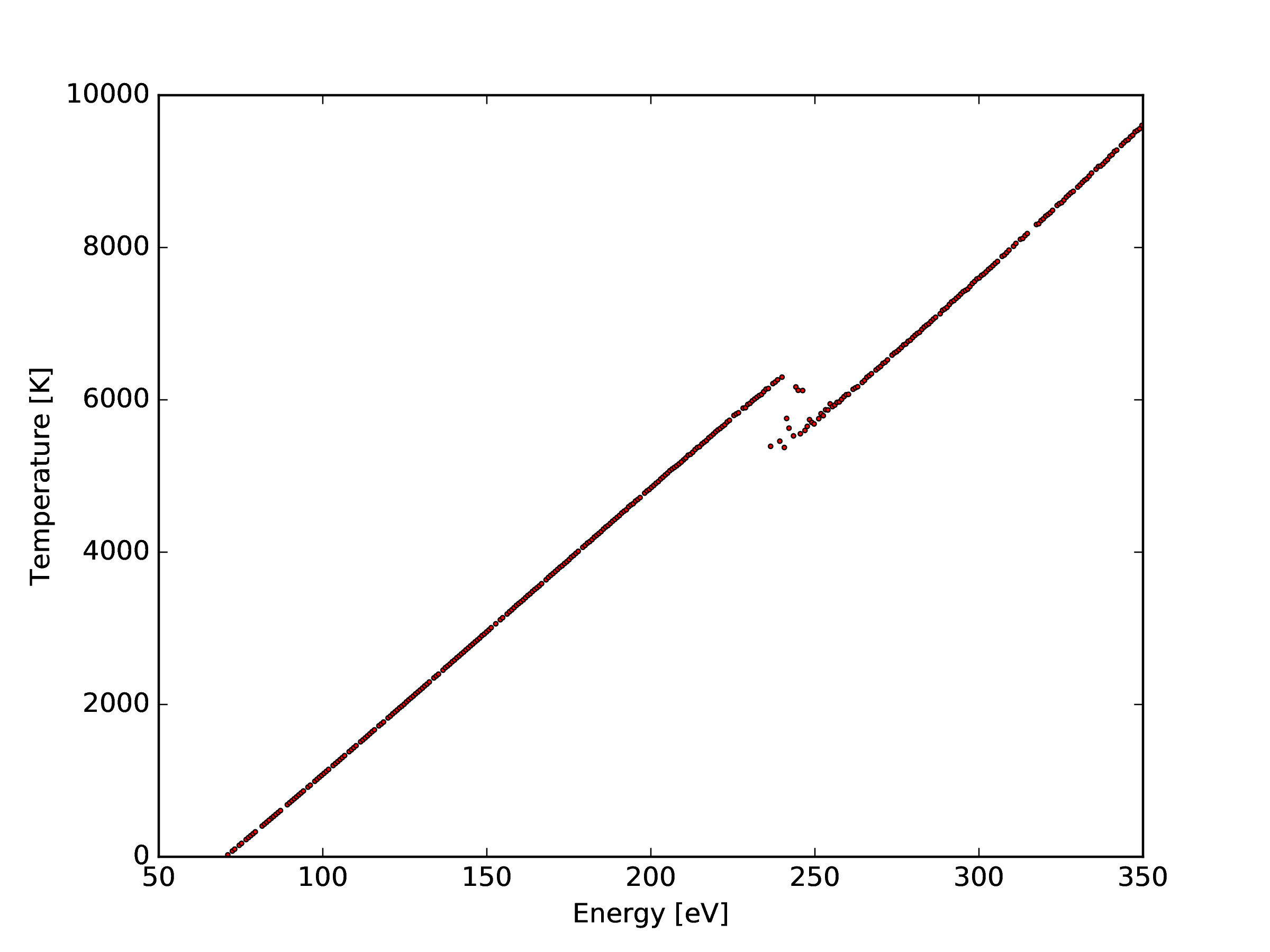
Figure 1: Isochoric (Z) curve obtained from 400 different 50 ps simulations of high-density Ar, with initial temperatures ranging from 50 to 20000 K. From this Z-curve we can determine $T_{m}\sim$ 5376 K and $T_{LS}\sim$ 6291 K. A clear drop of temperature is observed near the critical energy $E_{LS}\sim$ 240 eV.

From the isochoric, Z-shaped curve, we have estimated the melting temperature $T_{m}$ and the superheating limit $T_{LS}$. The sharp inflection at the higher temperature (6291 K) corresponds to $T_{LS}$ and the lower inflection (5376 K) corresponds to $T_{m}$. We can also determine $E_{LS}$ at approximately 240 eV.

Once $T_{LS}$ is estimated, at least 5000 classical MD runs were performed for 24 different initial temperatures $T_{0}$ in an interval from $T_{0}=$12075 K to $T_{0}=$13300 K, in order to collect statistically independent samples of waiting times. As it is known, by the equipartition theorem the initial temperature drops to around half the initial value when no velocity rescaling procedure or thermostat is used. If the specific heat at constant volume $C_{v}$ is independent of $T$ for the solid branch of the isochore, the temperature $T(E)$ is a linear function of the total energy $E$. Because $E$ is given by

$$E=\frac{3N}{2}k_{B}T_{0}+\Phi_{0}=E_{0}+C_{v}T,$$ (1)

we see that $T=m\;T_{0}+b$, in our case, $m$=0.40535 $\pm$ 0.004633 and $b$=1324.034 $\pm$ 56.37 K. The specific heat per atom is $3/(2m)$ in units of $k_{B}$, about 3.7.

As an example of the dynamical behavior of the instantaneous temperature $T(t)$ at the moment of melting, four realizations of MD simulation are shown, superimposed, in Fig. 2 for an initial temperature $T_{0}$=12800 K. Here we see the large variability of $t_{w}$ in those samples, ranging from approx. 5 ps to 30 ps.

From the MD simulations with duration $\tau_{0}$=50 ps we only considered for the collected statistics the values of $t_{w}$ such that $t_{w}\leq\tau_{0}$ (i.e. the simulatione were melting is not observed in the time window $\tau_{0}$ were ignored). Because of this, we are in fact inferring the truncated distribution $P(t_{w}|t_{w}\leq\tau_{0},T)$. For all simulations were melting is observed we extracted the temperature before and after the melting process, denoted by $T_{\text{solid}}$ and $T_{\text{liquid}}$ respectively, and the melting time $t_{w}$. This was done via a simple automated least-squares fitting using the following “discontinuous step” model,

$$T(t)=\begin{cases}T_{\text{solid}}&\;\text{if}\;t\leq t_{w},\\ T_{\text{liquid}}&\;\;\text{otherwise}.\end{cases}$$ (2)

For the lowest part of the range of initial temperatures, more precisely between 12000 K and 12250 K, 10000 simulations per temperature were performed instead of 5000. This is of course because the melting events are much less probable once we approach $T_{\text{solid}}=T_{LS}$ from above. In this way we have collected at least 200 samples of waiting times for each $T_{0}$.

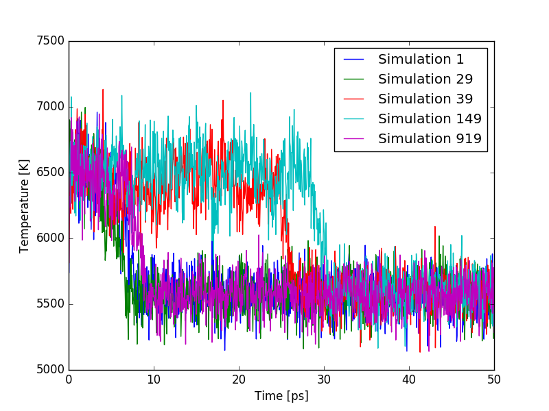
Figure 2: Instantaneous temperature $T(t)$ from five different simulations at an initial temperature $T_{0}=$12800 K. The melting process is triggered at different times $t_{w}$ between 5 and 30 ps for this particular energy.

In the next section we present a statistical description of $t_{w}$ for different initial temperatures, and a comparison of the exponential, gamma, log-normal and kernel density estimation (KDE) models against our data.

III Results

We have performed, for all 24 different initial temperatures $T_{0}$, a statistical analysis of the samples of melting time $t_{w}$ collected from several thousand MD simulations as described in the previous section. Figs. 3, 4 and 5 show the histograms of $t_{w}$ samples for increasing $T_{\text{solid}}$ above $T_{LS}$, together with their respective maximum likelihood exponential fit, with the exponential distribution given by

$$P(t_{w}|\lambda)=\lambda\exp(-\lambda t_{w})$$ (3)

with $\lambda$ a scale parameter, and a kernel density estimation.

We see in all cases that the exponential model cannot reproduce the left tail of the histogram, overestimating the probability of $t_{w}=0$. In contrast, this behavior is correctly reproduced by the kernel density method. Our results show that there is no instantaneous melting process, but a certain latency exists in which presumably some particular conditions in the crystal have to be set up. This can be explained by the fact that the collapse of the solid must involve the crossing of an energy barrier via a random walk in phase space.

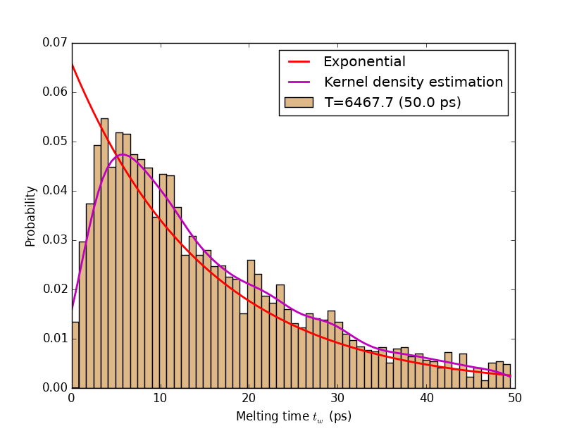
Figure 3: Probability density function for waiting times at $T_{0}$=12690 K ($T$=6467.7 K).

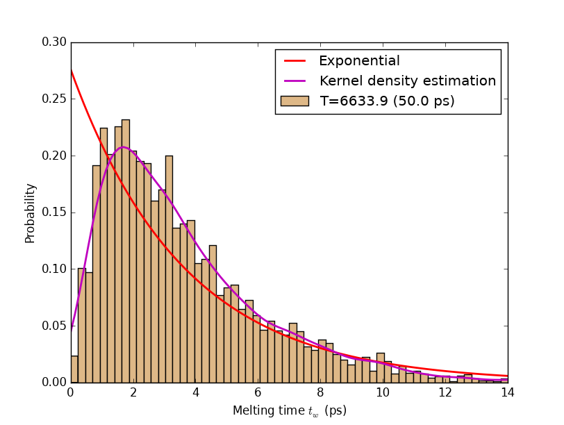
Figure 4: Probability density function for waiting times at $T_{0}$=13100 K ($T$=6633.9 K).

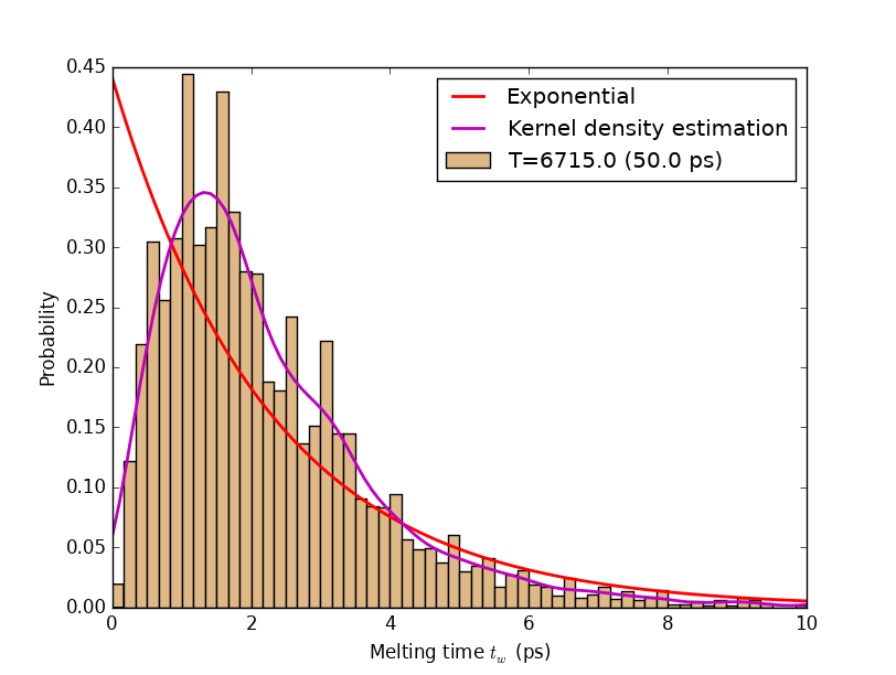
Figure 5: Probability density function for waiting times at $T_{0}$=13300 K ($T$=6715.0 K).

As expected, the most probable value of $t_{w}$ (i.e. its mode) decreases with the initial temperature, and the gap between the exponential and KDE models widens. We search, therefore, for an alternative statistical model with the same asymmetry observed in the histograms (long right tail) and with non-zero mode. We propose the gamma and log-normal models as candidates, which are assessed against the data in the next section.

IV Statistical models of waiting times and model comparison

At this point we consider as candidate statistical models for the waiting time $t_{w}$ the gamma distribution, given by

$$P(t_{w}|k,\theta)=\frac{\exp(-t_{w}/\theta)t_{w}^{k-1}}{\Gamma(k)\theta^{k}},$$ (4)

where $k$ and $\theta$ are the shape and scale parameters, respectively, and the log-normal distribution, given by

$$P(t_{w}|\mu,\sigma)=\frac{1}{\sqrt{2\pi}\sigma t_{w}}\exp\left(-\frac{1}{2\sigma^{2}}(\ln t_{w}-\mu)^{2}\right).$$ (5)

The comparison between these two models plus the exponential model, together with the kernel density estimation, is shown in Fig. 6. In this figure the goodness-of-fit of the models is also evaluated quantitatively using the Bayesian Information Criterion (BIC) Schwarz (1978). This criterion is based on computing the quantity

$$\text{BIC}=-2\ln L(\bm{\lambda_{0}})+n_{p}\ln n_{d},$$ (6)

where $L(\bm{\lambda})=P(\text{data}|\bm{\lambda})$ is the likelihood function for the model, $\bm{\lambda_{0}}$ is the parameter vector for which $L$ is maximum, $n_{p}$ is the number of parameters in the model and $n_{d}$ is the number of data points. Under this definition, the model with lowest BIC should be the most appropriate to represent the data. The first term favors models with high likelihood, while the second term penalizes the models with large number of parameters in order to avoid overfitting.

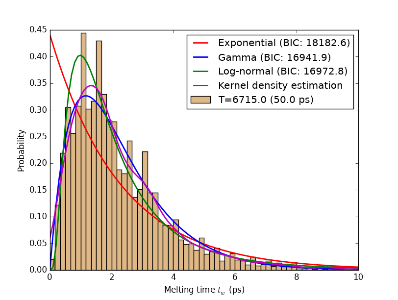
Figure 6: Comparison of exponential, gamma and log-normal models for waiting times at $T$=6715 K. The Bayesian Information Criterion (BIC) is reported for all models. Also a Gaussian kernel density estimation is included for reference.

We see that the lowest value of BIC is obtained by the gamma model, which is also visually the closest to the KDE reference model. Accordingly, we have chosen the gamma model as the basis of our further statistical description in the next section, where we incorporated the effect of truncation due to the limited duration of the MD simulations in the Z-method.

V The truncated gamma model

As was described previously, in every Z-method simulation there is an intrinsic truncation of the waiting times due to the finite duration of each run. We can incorporate this effect of truncation in the gamma model given by Eq. 4 as follows. The truncated probability density of $t_{w}$ is the conditional probability $P(t_{w}|t_{w}\leq\tau_{0},T)$, which due to Bayes’ theorem can be written as

$$P(t_{w}|t_{w}\leq\tau_{0},T)=\frac{P(t_{w}|T)P(t_{w}\leq\tau_{0}|t_{w},T)}{P(t_{w}\leq\tau_{0}|T)},$$ (7)

where $P(t_{w}|T)$ is given by Eq. 4 with $k=k(T)$ and $\theta=\theta(T)$. Moreover, the probability $P(t_{w}\leq\tau_{0}|t_{w},T)$ does not depend on $T$ and takes the value one if $t_{w}\leq\tau_{0}$, zero otherwise. So, it can be written as $\Theta(\tau_{0}-t_{w})$ for all values of $T$. Imposing normalization of the left-hand side of Eq. 7,

$$P(t_{w}\leq\tau_{0}|T) =\int_{0}^{\infty}dt_{w}P(t_{w}|T)\Theta(\tau_{0}-t_{w})$$

$$=\int_{0}^{\tau_{0}}dt_{w}P(t_{w}|T).$$ (8)

Combining Eqs. 4, 7 and 8 finally we arrive at

$$P(t_{w}|t_{w}<\tau_{0},T)=\frac{\exp(-t_{w}/\theta(T))t_{w}^{k(T)-1}\Theta(\tau_{0}-t_{w})}{\Gamma_{\text{inc}}(k(T);0\rightarrow\frac{\tau_{0}}{\theta(T)})\theta(T)^{k(T)}}$$ (9)

where $\Gamma_{\text{inc}}(k;a\rightarrow b)$ is the incomplete gamma function, given by

$$\Gamma_{\text{inc}}(k;a\rightarrow b)=\int_{a}^{b}dt\exp(-t)t^{k-1}.$$ (10)

Using this truncated model, we can compute several statistical properties of the waiting times. First, the probability of observing melting before a time $\tau_{0}$ at temperature $T$ is given by

$$P(t_{w}<\tau_{0}|T)=\frac{\Gamma_{\text{inc}}(k(T);0\rightarrow\frac{\tau_{0}}{\theta(T)})}{\Gamma(k(T))}.$$ (11)

Similarly, the most probable waiting time ${t_{w}}^{*}$ at a given $T$ is given by ${t_{w}}^{*}=(k(T)-1)\theta(T)$, while the average value of $t_{w}$ given a simulation time $\tau_{0}$ at a temperature $T$ is

$$\big{<}t_{w}\big{>}_{\tau_{0},T}=\theta(T)\left[\frac{\Gamma_{\text{inc}}(k(T)+1;0\rightarrow\frac{\tau_{0}}{\theta(T)})}{\Gamma_{\text{inc}(k(T);0\rightarrow\frac{\tau_{0}}{\theta(T)})}}\right],$$ (12)

which goes to $k(T)\theta(T)$ as $\tau_{0}\gg\theta(T)$, as expected.

All that remains for a complete statistical description is the estimation of the functions $k(T)$ and $\theta(T)$. We address this problem by means of Bayesian inference, first using a Bézier 50-parameter model (described in Appendix A) and a 7-parameter model, which we describe below.

Based on the original model by Alfè et al, we propose that for sufficiently high temperatures so that $\tau_{0}\gg\theta(T)$, i.e. when truncation effects are negligible and the probability of melting approaches one, the quantity

$$a(T)=\frac{1}{\sqrt{\big{<}t_{w}\big{>}_{T}}}$$ (13)

increases linearly with $T$. However, at low temperatures it saturates, as seen in the simulation data (Figure 7, circles).

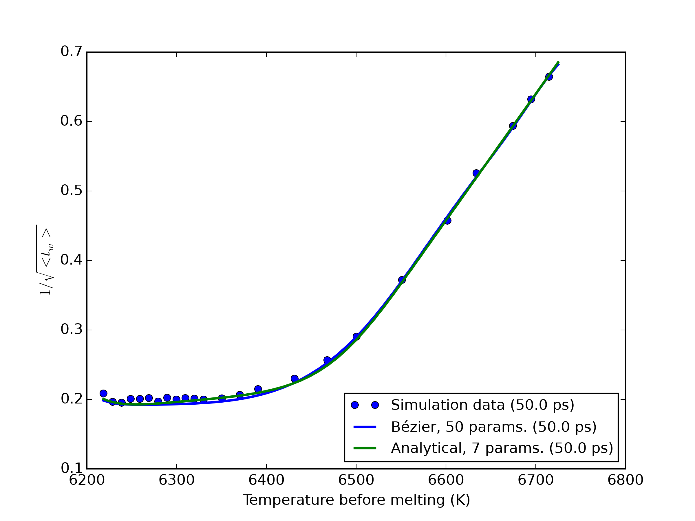
Figure 7: The quantity $1/\sqrt{\big{<}t_{w}\big{>}_{T}}$ as a function of $T$. Circles represent simulation points with $\tau_{0}$=50 ps, while the blue and green lines are the Bézier and 7-parameter analytical models proposed in this work, respectively. We see that the linear behavior for high temperatures is no longer valid below a certain temperature $T^{*}$, in this case approximately 6550 K.

Accordingly, we will define an “inflection temperature” $T^{*}$ that separates both regimes, in such a way that $a(T)$ is given by

$$a(T)=\begin{cases}C+R(T-T_{\text{base}})^{\gamma}&\;\text{if}\;T\leq T^{*},\\ \alpha T-\beta&\;\;\text{otherwise}.\end{cases}$$ (14)

where the parameter $T_{\text{base}}$ is a reference temperature, fixed here at 6200 K, and the parameters $R$ and $C$ are fixed by the continuity of $a(T)$ and its derivative at $T^{*}$ as

$$R=\frac{\alpha}{\gamma(T^{*}-T_{\text{base}})^{\gamma-1}},$$

$$C=\alpha T^{*}-\beta-R(T^{*}-T_{\text{base}})^{\gamma}.$$ (15)

As $\big{<}t_{w}\big{>}_{T}=k(T)\theta(T)$ for a gamma-distributed $t_{w}$, it follows that

$$k(T)=\frac{1}{\theta(T)a(T)^{2}}.$$ (16)

Now, the behavior of $\theta(T)$ is monotonically decreasing with $T$, and on first thought an Arrhenius law would be expected. In fact, however, it deviates from an exponential and we added a quadratic dependence on $\ln\theta(T)$,

$$\ln\theta(T)=\ln\theta_{0}-\left(\frac{T-T_{\min}}{\eta}\right)-\left(\frac{T-T_{\min}}{\zeta}\right)^{2}.$$ (17)

Parameter	Confidence interval	Uncertainty %
$T^{*}$ (K)	6550.02 $\pm$ 1.80	0.0275%
$\gamma$	1.8487 $\pm$ 0.0051	0.276%
$\theta_{0}$ (ps)	2667.51 $\pm$ 96.03	3.600%
$\eta$ (K)	40.48 $\pm$ 0.39	0.963%
$\zeta$ (K)	231.75 $\pm$ 2.23	0.962%
$\alpha$ (ps-1/2K-1)	1.8198$\times$10-3 $\pm$ 1.02$\times$10-6	0.056%
$\beta$ (ps-1/2)	11.5446 $\pm$ 0.0065	0.0563%

Table 1: Estimated parameters for the analytical model given by Eqs. 14 to 17. The confidence intervals reported are constructed using the mean and standard deviation of Markov Chain Monte Carlo samples from the posterior distribution.

Finally, we have that the functions $k(T)$ and $\theta(T)$ are described by 7 parameters in total, namely $T^{*}$, $\gamma$, $\theta_{0}$, $\eta$, $\zeta$, $\alpha$ and $\beta$. These are in fact hyperparameters for the gamma distribution, and were estimated given our simulation data using a Bayesian Markov Chain Monte Carlo (MCMC) procedure, described in detail in Appendix B.

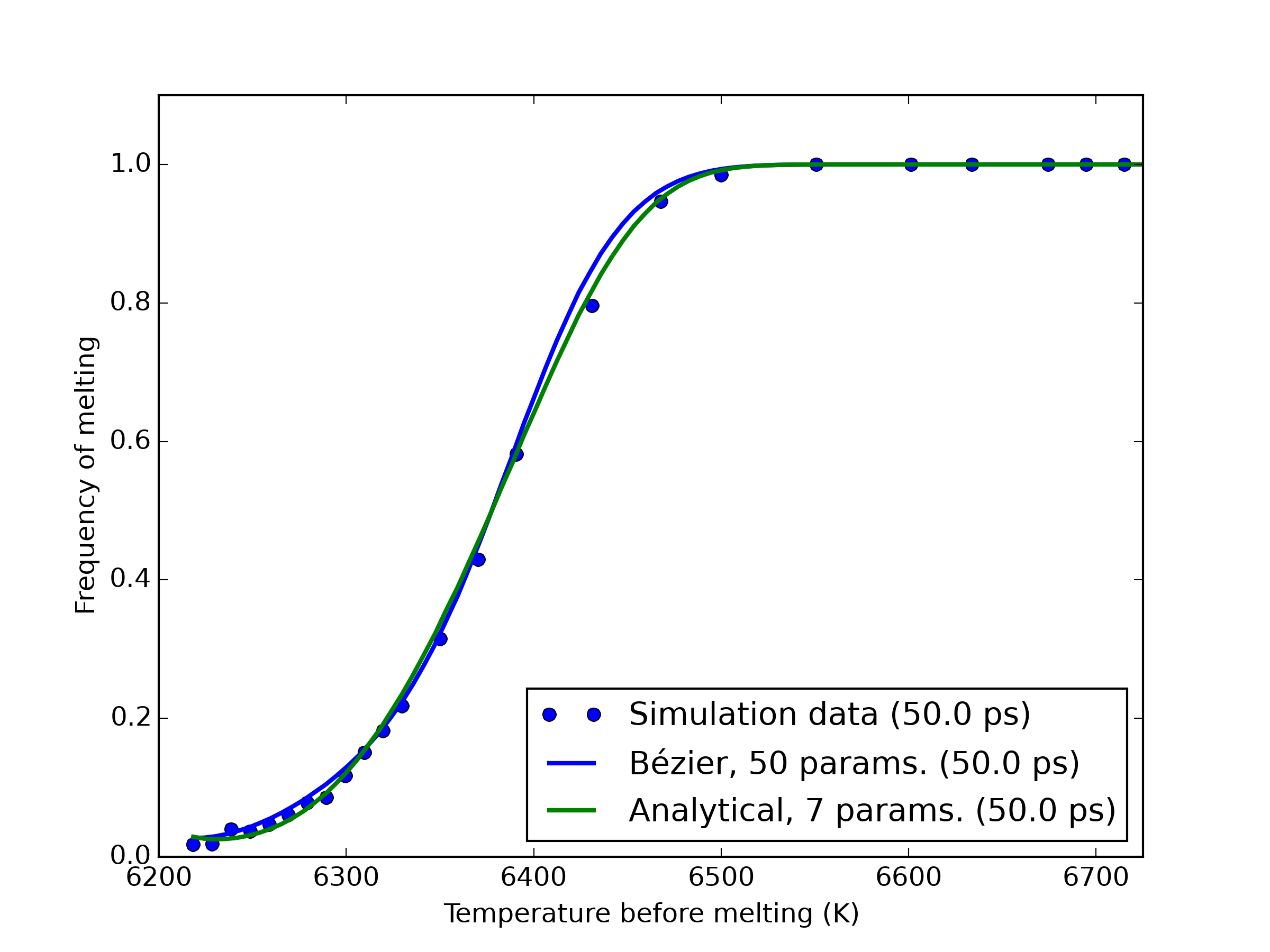
Figure 8: Frequency of melting (Eq. 11) as a function of $T$ for the truncated gamma model. Circles represent the simulation data with $\tau=$50 ps, while the blue and green lines are the Bézier and 7-parameter analytical models proposed in this work, respectively.

The confidence intervals for all parameters from this procedure are summarized in Table 1. For all parameters the uncertainty is below 4%, and in some cases well below 1%. Fig. 8 shows the agreement of the same models on the frequency of melting as a function of $T$, while Fig. 9 shows the agreement of the two models (Bézier and 7-parameter) against the simulation data on the truncated parameters $k(T)$, $\theta(T)$ and $\big{<}t_{w}\big{>}_{T,\tau_{0}}$. In both cases we see a remarkable agreement with the simulation, with the Bézier model providing the best fit due to the large number of parameters. The 7-parameters model seems to be precise enough in its predictions for practical use.

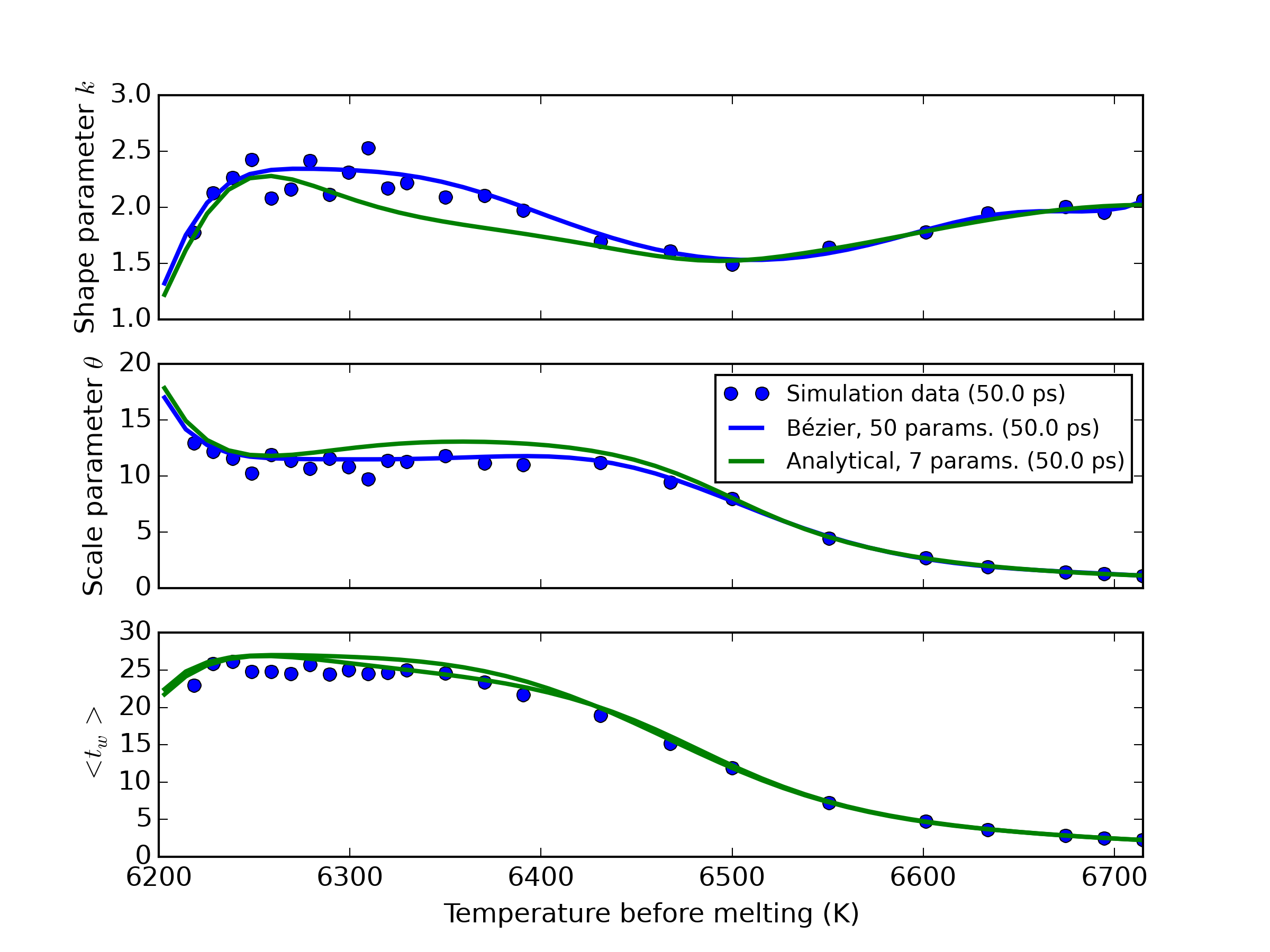
Figure 9: Parameters $k(T)$, $\theta(T)$ and the expected waiting time $\big{<}t_{w}\big{>}_{T,\tau_{0}}$ for the truncated gamma model. Circles represent the simulation data with $\tau=$50 ps, while the blue and green lines are the Bézier and 7-parameter analytical models proposed in this work, respectively.

Figs. 10, 11 and 12 show the Bayesian posterior distribution functions sampled using the MCMC procedure. For all parameters except $\alpha$ and $\beta$ the posterior distribution has been resolved clearly, and is unimodal with a well-defined shape. In the case of $\alpha$ and $\beta$ the uncertainty is so small (approx. 0.056%) that the MCMC procedure does not resolve the shape of the peak. However, this is of no importance, because for such a small uncertainty a point estimate contains essentially all the information about the distribution.

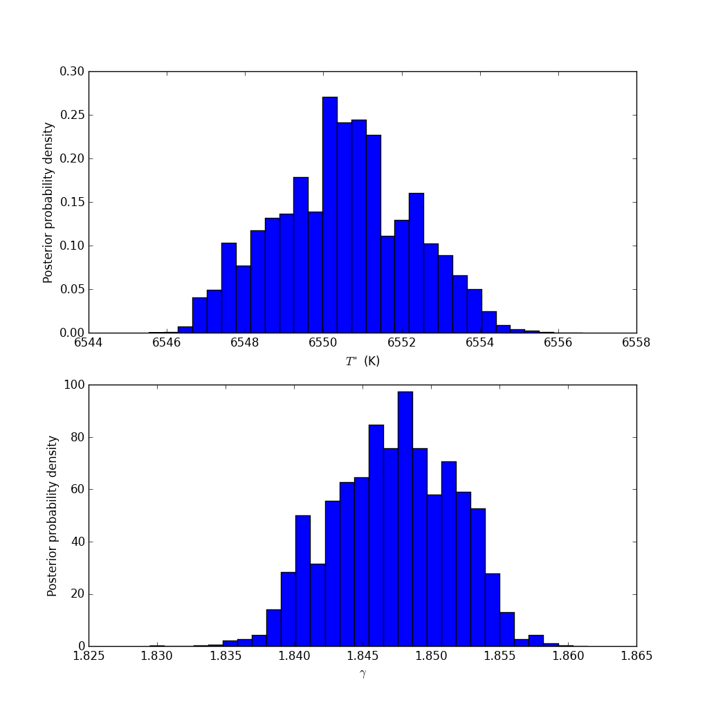
Figure 10: Bayesian posterior densities for the parameters $T^{*}$ and $\gamma$.

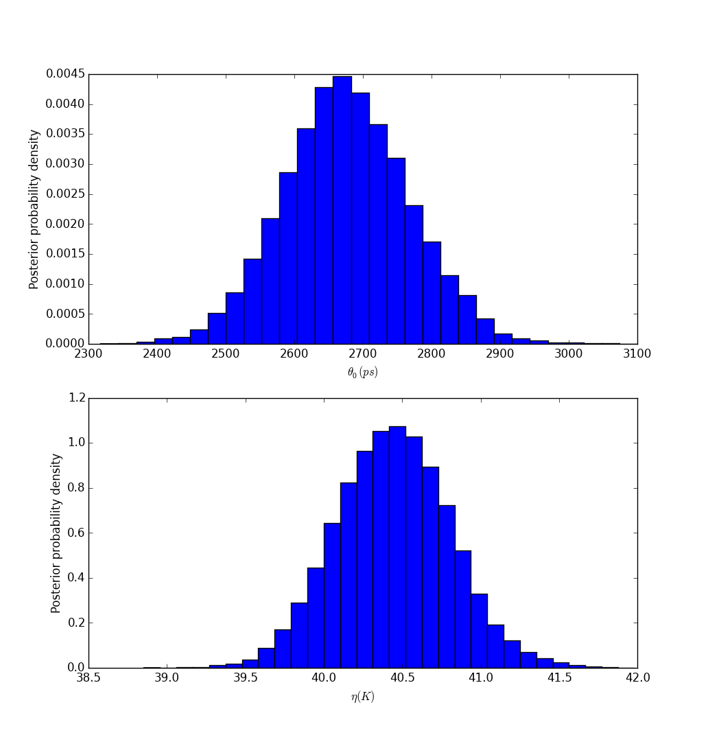
Figure 11: Bayesian posterior densities for the parameters $\theta_{0}$ and $\eta$.

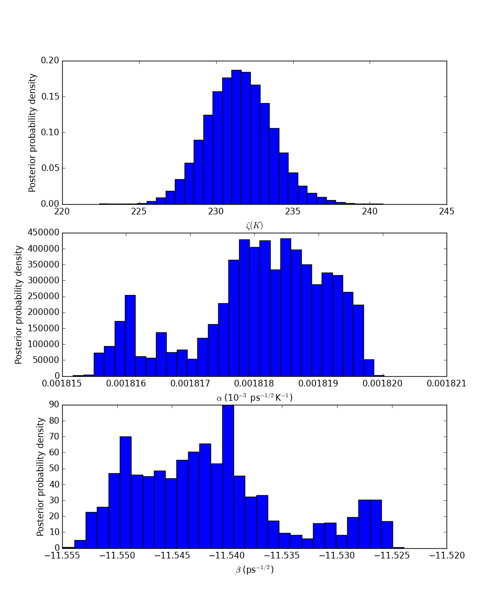
Figure 12: Bayesian posterior densities for the parameters $\zeta$, $\alpha$ and $\beta$.

VI Concluding remarks

We have presented a detailed statistical description of the waiting times in homogeneous, microcanonical melting as a function of initial energy. The 7-parameter model, together with their uncertainties, was constructed by using a large set of 80000 independent molecular dynamics simulations and the application of Bayesian inference techniques. Our results shows that the waiting time $t_{w}$ is gamma-distributed, not exponential, with a well-defined probability maximum at non-zero times. We interpreted this as the absence of instantaneous melting due to the intrinsic latency caused by the initial random exploration in phase space, prior to the crossing of an energy barrier.

The model we present here could be of use not only for further understanding of the microcanonical melting in ideal conditions, but also in situations where ultrafast melting occurs, in which the time and length scales are so short that essentially a microcanonical situation arises. Two examples with technological relevance are laser-induced melting Plech et al. (2004); Musumeci et al. (2010); Siwick et al. (2003) and melting produced by radiation Shirokova et al. (2013); Inestrosa-Izurieta et al. (2015) impacting on surfaces.

It would be interesting to explore the possibility that the parameters of the model given in Table 1 can be normalized in a universal way with a natural temperature scale in terms of $T_{m}$ and $T_{LS}$, and a natural time scale adequate for the system (for a fixed system size).

Appendix A Bézier model for the gamma parameters

We described the functions $k(T)$ and $\theta(T)$ by expanding them in a polynomial basis known as Bernstein polynomials. This expresses the curves $k$ and $\theta$ as Bézier curves, parameterized by

$$k(T)=\sum_{i=0}^{24}A_{i}\binom{n}{i}\mathcal{T}^{i}(1-\mathcal{T})^{n-i},$$

$$\theta(T)=\sum_{i=0}^{24}B_{i}\binom{n}{i}\mathcal{T}^{i}(1-\mathcal{T})^{n-i},$$ (18)

where $\mathcal{T}$ is a normalized temperature (between 0 and 1), defined for convenience as

$$\mathcal{T}=\frac{T-T_{\text{min}}}{T_{\text{max}}-T_{\text{min}}}.$$ (19)

In our case we have used $T_{\min}$=6200 K and $T_{\max}$=6700 K. For this model the hyperparameters describing $k$ and $\theta(T)$ are the coefficients $A_{i}$ and $B_{i}$, with $i$=0,…,24, leading to a total of 50 parameters.

Appendix B Markov Chain Monte Carlo

We employed a log-likelihood function divided into two terms. The first involves the data from melting times at a temperature $T_{i}$, and is given by

$$\ln P(M_{i}|k,\theta)=n_{i}\Big{(}-\frac{t_{i}}{\theta(T_{i})}+(k(T_{i})-1)L_{i}$$

$$-\ln\Gamma_{\text{inc}}(k(T_{i});0\rightarrow\frac{\tau_{0}}{\theta(T_{i})})-k(T_{i})\ln\theta(T_{i})\Big{)},$$ (20)

where $n_{i}$ is the number of ocurrences of melting at $T_{i}$ (from a total of $N_{i}$), $t_{i}$ and $L_{i}$ denote the sample averages at $T_{i}$ of $t_{w}$ and $\ln t_{w}$, respectively. The second contribution to the total log-likelihood includes the number of realizations of melting $n_{i}$ and the total number of realizations $N_{i}$ at temperature $T_{i}$, and is given by

$$\ln P(F_{i}|k,\theta)=n_{i}\ln p_{i}-(N_{i}-n_{i})\ln(1-p_{i})$$

$$+\ln\left[\frac{N_{i}!}{n_{i}!(N_{i}-n_{i})!}\right],$$ (21)

with $p_{i}=P(t_{w}<\tau_{0}|T_{i})$ the predicted probability of melting at temperature $T_{i}$. The logarithm of the posterior distribution of parameter functions $k$ and $\theta$ is then given by

$$\ln P(k,\theta|\{M_{i},F_{i}\})=\sum_{i=1}^{m}\Big{(}\ln P(M_{i}|k,\theta)+\ln P(F_{i}|k,\theta)\Big{)},$$ (22)

with flat uninformative priors. This logarithm of the posterior distribution was sampled using a Markov Chain Monte Carlo (MCMC) methodology, namely Metropolis-Hastings sampling Gamerman and Lopes (2006), over the hyperparameters present in the models given by Eqs. 16, 17 and 18.

References

- Forsblom and Grimvall (2005) M. Forsblom and G. Grimvall, Nature Materials 4, 388 (2005).
- Siwick et al. (2003) B. J. Siwick, J. R. Dwyer, R. E. Jordan, and R. J. Miller, Science 302, 1382 (2003).
- Belonoshko et al. (2006) A. B. Belonoshko, N. V. Skorodumova, A. Rosengren, and B. Johansson, Phys. Rev. B 73, 012201 (2006).
- Belonoshko et al. (2007) A. B. Belonoshko, S. Davis, N. V. Skorodumova, P. H. Lundow, A. Rosengren, and B. Johansson, Phys. Rev. B 76, 064121 (2007).
- Pozo et al. (2015) M. J. Pozo, S. Davis, and J. Peralta, Physica B 457, 310 (2015).
- Bai and Li (2008) X.-M. Bai and M. Li, Physical Review B 77, 134109 (2008).
- Davis et al. (2011) S. Davis, A. B. Belonoshko, B. Johansson, and A. Rosengren, Physical Review B 84, 064102 (2011).
- Samanta et al. (2014) A. Samanta, M. E. Tuckerman, T.-Q. Yu, and W. E, Science 346, 729 (2014).
- González-Cataldo et al. (2016) F. González-Cataldo, S. Davis, and G. Gutiérrez, Sci. Rep. 6, 26537 (2016).
- Belashchenko (2013) D. K. Belashchenko, Physics-Uspekhi 56, 1176 (2013).
- Belonoshko et al. (2009) A. B. Belonoshko, P. M. Derlet, A. S. Mikhaylushkin, S. I. Simak, O. Hellman, L. Burakovsky, D. C. Swift, and B. Johansson, New Journal of Physics 11, 093039 (2009).
- Alfè et al. (2011) D. Alfè, C. Cazorla, and M. J. Gillan, J. Chem. Phys. 135, 024102 (2011).
- Davis et al. (2010) S. Davis, C. Loyola, F. González, and J. Peralta, Comp. Phys. Comm. 181, 2126 (2010).
- Schwarz (1978) G. E. Schwarz, Annals of Statistics 6, 461 (1978).
- Plech et al. (2004) A. Plech, V. Kotaidis, S. Grésillon, C. Dahmen, and G. von Plessen, Phys. Rev. B 70, 195423 (2004).
- Musumeci et al. (2010) P. Musumeci, J. T. Moody, C. M. Scoby, M. S. Gutierrez, and M. Westfall, Appl. Phys. Lett. 97, 063502 (2010).
- Shirokova et al. (2013) V. Shirokova, T. Laas, A. Ainsaar, J. Priimets, U. Ugaste, E. V. Demina, V. N. Pimenov, S. A. Maslyaev, A. V. Dubrovsky, V. A. Gribkov, et al., J. Nucl. Mat. 435, 181 (2013).
- Inestrosa-Izurieta et al. (2015) M. J. Inestrosa-Izurieta, E. Ramos-Moore, and L. Soto, Nucl. Fusion 55, 093011 (2015).
- Gamerman and Lopes (2006) D. Gamerman and H. F. Lopes, Markov Chain Monte Carlo: Stochastic Simulation for Bayesian Inference (Taylor and Francis, 2006).