Automatic HVAC Control with Real-time Occupancy Recognition and Simulation-guided Model Predictive Control in Low-cost Embedded System

Abstract

Intelligent building automation systems can reduce the energy consumption of heating, ventilation and air-conditioning (HVAC) units by sensing the comfort requirements automatically and scheduling the HVAC operations dynamically. Traditional building automation systems rely on fairly inaccurate occupancy sensors and basic predictive control using oversimplified building thermal response models, all of which prevent such systems from reaching their full potential. Such limitations can now be avoided due to the recent developments in embedded system technologies, which provide viable low-cost computing platforms with powerful processors and sizeable memory storage in a small footprint. As a result, building automation systems can now efficiently execute highly-sophisticated computational tasks, such as real-time video processing and accurate thermal-response simulations. With this in mind, we designed and implemented an occupancy-predictive HVAC control system in a low-cost yet powerful embedded system (using Raspberry Pi 3) to demonstrate the following key features for building automation: (1) real-time occupancy recognition using video-processing and machine-learning techniques, (2) dynamic analysis and prediction of occupancy patterns, and (3) model predictive control for HVAC operations guided by real-time building thermal response simulations (using an on-board EnergyPlus simulator). We deployed and evaluated our system for providing automatic HVAC control in the large public indoor space of a mosque, thereby achieving significant energy savings.

1 Introduction

Heating, ventilation, and air-conditioning (HVAC) units, which are a primary target of building automation, make up almost 50% of the energy consumed in both residential and commercial buildings [1]. In general, building automation systems aim to intelligently control building facilities in response to dynamic environmental factors, while maintaining satisfactory performance in energy consumption and comfort. The primary functions of a building automation system include: (1) sensing of the environmental factors by measurements, and (2) optimizing control strategies based on the current and predictive states of building and occupancy. These tasks require an integrated process of sensing, computation, and control.

Traditional building automation systems rely on fairly inaccurate occupancy sensors, which hinder the responsiveness of automation systems. For example, passive infrared and ultra-sound occupancy sensors produce poor accuracy, because they are unable to determine the occupancy state adequately when occupants remain stationary for a prolonged period of time. They also have a limited range which hinders their performance, especially in a large area. More accurate sensing technology, such as cameras that use visible or infra-red lights, can significantly improve the accuracy of occupancy recognition.

On the other hand, model predictive control, by which the future thermal response and external environmental factors are anticipated to make control decisions accordingly, has been considered in a number of studies [2, 3, 4, 5, 6, 7] which are shown to be more effective than classical PID and hysteresis controllers that do not consider anticipated events. However, these studies are often based on time-invariant, first-principle linear models (also known as lumped element resistance-capacitance (RC) models [8]), considering only simple building geometry and single-zone in near-future time horizon. Although these linear models are easier for calibration (e.g., using frequency domain decomposition, or subspace system identification methods [8, 9, 10]), the error accumulates considerably when a longer time horizon is considered in model predictive control. While non-linear models are rather complicated and impractical, other alternatives based on physical models of building thermal response can provide a feasible solution.

Recently, there have been remarkable advances in embedded system technologies, which provide low-cost platforms with powerful processors and sizeable memory storage in a small footprint. In particular, the emergence of system-on-a-chip technology [11], which integrates all major components of a computer into a single chip, can provide versatile computing platforms with low-power consumption and mobile network connectivity in a cost-effective manner for mass production. As a result, smartphones are able to rapidly evolve from single-core to multi-core processors with a low incremental production cost. Notably, the Raspberry Pi project [12], which originally aimed to provide affordable solutions for the teaching of computer science, has rapidly evolved for a wide range of advanced scientific projects. Therefore, there are plenty of opportunities to harness recent embedded system technologies in intelligent building automation systems. Particularly, sophisticated computational tasks can be conducted on these embedded systems efficiently, such as real-time video processing and accurate building thermal response simulation (e.g., [13]).

With this in mind, we designed and implemented an occupancy-predictive HVAC control system in a low-cost yet powerful embedded system (using Raspberry Pi 3) for building automation. The rest of the paper is organized as follows. In Section 2, we present the background information and literature review. In the remaining sections, we highlight three key features of our system.

(Section 3) Real-time Video-based Occupancy Recognition

We apply advanced video-processing techniques to analyze the features of occupants from video cameras, and automatically classify and infer the states of occupancy. Moreover, we consider privacy enhancement using a frosted lens. Our system achieves 80-90% accuracy for occupancy recognition by real-time video processing. Furthermore, we improve the performance of our occupancy recognition by using Machine Learning for considerably crowded settings.

(Section 4) Dynamic Occupancy Prediction

We employ various linear and non-linear regression models to capture and predict occupancy trends according to different day-of-week, seasonal patterns, etc. We present general as well as domain-specific approaches for occupancy prediction. Our models are able to identify the future occupancy trends considering a variety of dynamic usage patterns.

(Sections 5-6) Simulation-guided Model Predictive Control

We employ EnergyPlus simulator [14] for real-time HVAC control. We ported EnergyPlus simulator to the Raspberry Pi embedded system platform for simulation-guided model predictive control. A co-simulation framework is utilized to provide accurate building thermal response simulation under proper calibration. Noteworthily, we also release our Raspberry Pi version of EnergyPlus publicly [15] to enable other researchers to take advantage of our work for future building automation projects.

Our automatic HVAC control system is intended for public indoor spaces, such as corridors, libraries, or communal areas. Unlike private spaces such as homes, these public indoor spaces are not controlled by a particular occupant and can be affected by a diverse set of occupancy patterns. Such patterns tend to vary more dynamically in public spaces compared to private ones, posing challenges for effective occupancy sensing and prediction systems.

In particular, our system is deployed and evaluated for providing automatic HVAC control in the large public indoor space of a mosque (see Figure 1), which is the worship place for followers of Islam. Typically, mosques have large public spaces, and are open 24-hours a day and 7-days a week. There are nearly 5,000 mosques in the UAE [16], and over 55,000 mosques in Saudi Arabia [17]. Due to the hot climate in this region, HVAC is required on a regular basis. The results obtained from our testbed implementation in Section 7 demonstrate the significant energy savings that can be achieved by using automatic HVAC control systems in public indoor spaces.

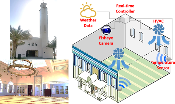
Figure 1: A large public indoor space of a mosque is used as a testbed for our automatic HVAC control system. Fisheye video camera, temperature and humidity sensors, as well as real-time controller for HVAC have been deployed in our testbed.

2 Background and Related Work

In this section, we present the background and related work of our system. In particular, this section consists of two subsections. The first provides a brief review of occupancy recognition and prediction. The second subsection compares three main approaches of model predictive HVAC control.

2.1 Occupancy Recognition and Prediction

Any object with a temperature higher than perfect zero emits heat in the form of radiation. The conventional passive infra-red (PIR) sensors can be used to detect a certain wavelength when a person is near the sensor. Previous papers [18, 19, 20] demonstrated the possibility of applying this to control lighting systems. However, the disadvantage of the PIR sensor becomes evident when the occupant remains stationary for a certain period of time. In particular, PIR sensors are designed to detect changes in the movement, and if a person remains stationary in front of the sensor, then as far as the sensor is concerned, there will be no change in the movement, leading to an erroneous observation.

Video-based occupancy-detection algorithms can provide better accuracy than their PIR counterparts. One such algorithm was proposed in [21], whereby certain features (such as edges, textures, etc.) are extracted from the video and used in a regression model to estimate the number of occupants. Unfortunately, this algorithm is computationally intensive, rendering it unsuitable for implementations on embedded systems such as Raspberry Pi. In contrast, our algorithm can detect occupancy in real-time, even when implemented on an embedded system, as is the case with our testbed. An alternative algorithm was proposed in [22]. Although this algorithm is computationally less intensive than the previous one, it nevertheless relies heavily on identifying the heads of the occupants. This head-detection process is particularly challenging in our testbed, as it is common for a typical occupant to have a head cover indistinguishable from his or her outfit. Since our system does not require head detection, it is insensitive to whether or not the occupant is wearing a head cover.

In addition to occupancy recognition, occupancy prediction is required to anticipate building usage and control pre-cooling in advance. A variety of techniques to predict occupancy have been proposed in the literature, including statistical analysis, machine learning, and stochastic modeling. A comprehensive review of occupancy prediction techniques is provided in [23, 24].

2.2 Model Predictive Control

There are three major approaches to model predictive control in the literature:

• LTI Model Predictive Control: This uses a linear time-invariant (LTI) mathematical model, which is a simplified thermal dynamics model considering only a near-future short time horizon. A common approach is to use an RC model to capture the first-order heat transfer dynamics. It is suitable for simple settings, such as a single zone with simple building geometry. There are usually a small number of parameters in the model. LTI model predictive control is explored in [8, 9, 10, 25, 26].

• Non-linear Model Predictive Control: Many real-world systems exhibit rich non-linearity. There are many general non-linear mathematical models of system dynamics, such as Volterra series, neural networks and NARMAX models. However, most non-linear models require a large parameter space, which is difficult to calibrate from measurements. The use of non-linear models for predictive control is investigated in [27, 28].

• Simulation-guided Model Predictive Control: In this approach, model predictive control is guided by real-time physical model simulators considering future anticipated events. For buildings, there are a number of simulators, such as EnergyPlus and TRNSYS, that are much more accurate than LTI models, and also easier to calibrate than general non-linear models. Reviews of different building simulators and their merits are presented in [5, 29].

For the above control approaches to be effective, it is crucial to calibrate the model parameters so that the model response is consistent with the empirical data. Several model calibration methods have been proposed in the literature. These methods can be broadly categorized as manual or automated. In particular, manual approaches require the modeler to intervene repeatedly and make adjustments, whereas automated approaches use mathematical and statistical models to automate the calibration process. A review of model calibration can be found in [30].

Several previous studies used simulation programs to facilitate model predictive control. Specifically, in [5, 7, 31], the authors employed co-simulation for model predictive control (MPC) with EnergyPlus. However, these studies did not implement the MPC models in real-world HVAC systems and were limited to simulations. Other studies [32, 33] tested the MPC models with real-world HVAC systems, but relied on powerful desktop computers running costly numerical computation software such as MATLAB.

There are other studies using occupancy prediction for MPC in HVAC systems. For example, [34, 25, 35, 26] used machine learning to predict occupancy patterns based on environmental sensor data. More specifically [34] and [35] used predicted occupancy patterns to simulate HVAC control in EnergyPlus, whereas [25, 26] developed LTI MPC algorithms for HVAC control in real buildings. Furthermore, [36] investigated the potential benefits of occupancy information for HVAC control, but their investigation was only limited to simulations.

The differences between our study and the aforementioned studies are: (1) we implemented our MPC algorithm in a real-world testbed using free-software platforms and low-cost embedded systems; (2) we employed EnergyPlus for real-time simulation-guided MPC of HVAC systems; (3) we developed a comprehensive solution that integrates occupancy recognition, occupancy prediction and simulation-guided MPC, thereby demonstrating the viability of automatic HVAC control using low-cost embedded systems.

3 Occupancy Recognition

Occupancy information is crucial for many applications, such as building management and human behavior studies. We develop an occupancy recognition system based on real-time video processing of a video stream to infer the occupancy patterns dynamically. This raises a number of challenges. First, structures differ from one building to another, leading to the possibility of occupants being obscured by various obstacles, such as pillars. Hence, we need to track the movements of occupants to determine the occupancy more accurately. Second, our algorithm is executed on an embedded system (e.g., Raspberry Pi), which has limited processing power and memory space compared to a typical desktop computer; this is particularly challenging since the typical video-processing algorithms are computationally demanding.

The basic idea of our occupancy-recognition algorithm is to count the number of people crossing a virtual reference line in the video, captured by a fisheye camera. Objects are identified as moving blobs (i.e., a set of connected points whose position is changing during the video stream); every such blob is interpreted as a person. Whenever a moving blob is detected, the algorithm keeps track of its movement to determine whether it passes the virtual reference line, and then updates the number of occupants accordingly. In particular, we position the line near the entrance of the space. Whenever the moving blob passes inward, the total number of occupants is increased by 1, and whenever the moving blob passes outward, the total number of occupants is decreased by 1.

Our algorithm consists of the following five steps: (1) background isolation, (2) silhouette detection, (3) object tracking, (4) inward/outward logging, and (5) inconsistency resolution. The flowchart of our algorithm is presented in Figure 2. In our implementation, two open-source projects were used: OpenCV [37] and openFramework [38]. Next, we will explain each step in details.

Figure 2: Flowchart of our occupancy-recognition algorithm.

3.1 Background Isolation

The purpose of background isolation is to identify a background image in the current video frame. Note that the appearance of the background may vary over the course of the video, depending on the time-of-day (e.g., turning on the lights at night may significantly alter the appearance of the background compared to natural light). The shadows of occupants must also be taken into consideration during the background isolation. To overcome these challenges, we employ the Gaussian mixture-based background/foreground segmentation algorithm proposed in [39, 40], and implemented on OpenCV.

3.2 Silhouette Detection

In our setting, the term “silhouette” is used to refer to the border of a set of continuous points. Silhouette detection is based on the algorithm proposed in [41]. The silhouettes of moving objects are extracted by comparing the current frame with the previous one; see Figure 3 for some examples. Here, only the silhouettes larger than a certain threshold area, $A$, are considered. The threshold is adjusted depending on the viewpoint and orientation of the camera. Furthermore, we use different values of $A$ for different parts of the space, to reflect the fact that individuals appear smaller as they move farther away from the camera. Importantly, the silhouettes of two or more people may overlap, and may, therefore, be interpreted as only one individual. To overcome this challenge, we use a machine-learning technique which will be explained later on in Section 3.6.

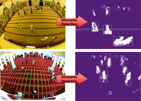
Figure 3: Examples of silhouette detection, taken from different buildings in which our system is deployed.

3.3 Object Tracking

After obtaining the silhouettes of occupants, their bounding boxes are logged for tracking. To this end, the list ${T_{a}}$ of silhouettes from the last frame is maintained. The algorithm then obtains the list ${T_{b}}$ of silhouettes from the current frame. For each bounding box $B_{b}$ in ${T_{b}}$, the algorithm determines whether there exists a box $B_{a}$ in $T_{a}$ that is within a certain distance, $d$, from $B_{b}$. If so, then $B_{b}$ is assumed to be the new location of $B_{a}$. Consequently, $B_{a}$ is updated in $T_{a}$, and its location is set to be that of $B_{b}$, in preparation for the next iteration of the algorithm. Note that the silhouettes are detected when they are moving. However, in cases where people might stop for a few seconds and then continue to walk, those objects will be removed from $T_{a}$ when they are missed for a certain number of seconds.

3.4 Inward/Outward Logging

Given the collection of moving objects and their locations, a virtual reference line is used to count occupants. Specifically, whenever the locations are updated, the algorithm checks every object to determine whether that object has crossed from one side of the line to the other. If so, then the number of occupants is updated according to the direction of the movement. For inward movement, the number of occupants increases by 1, otherwise it decreases by 1. Furthermore, since the silhouettes of any two moving objects may overlap, the width of the bounding box can be used to infer the number of occupants contained in each object.

3.5 Inconsistency Resolution

With all the techniques described thus far, the performance of the algorithm may not be satisfactory, due to one major challenge: the silhouettes of different occupants may overlap. In this case, some of the overlapping occupants may go undetected by the algorithm. This problem becomes even more evident when the movement patterns are affected by whether the occupants are entering or leaving the building, e.g., due to the fact that occupants arrive one by one, but leave all at once. For instance, in our application domain, the pace at which people leave is significantly faster than the pace at which they enter. Consequently, when all occupants leave at once, the number of overlapping silhouettes increases, leading to a larger number of people going undetected by the algorithm. As a result, the algorithm on average misses more occupants leaving than entering the building, leading to the erroneous conclusion that there are still occupants in the building when in fact there are none.

To resolve such inconsistency, two simple techniques are used. First, if the number of occupants becomes negative, the occupant counter is frozen until another object crosses the reference line inward. Second, if no moving object is detected for a certain period of time, the occupant counter is reset to zero. While these simple techniques reduce the error, they are clearly insufficient. In Section 3.6, we propose a dedicated technique to address this issue.

3.6 Improvement by Machine Learning

As mentioned earlier, one of the major challenges that we have encountered while deploying our occupancy-detection algorithm is to resolve the problem of overlapping silhouettes. One solution is based on the width of bounding box; the wider the box, the more occupants it contains. However, we observe that such a solution is insufficient, especially when an occupant happens to be directly in front of another. To resolve this issue, we employ machine-learning and image-classification techniques, coupled with randomized principal component analysis (PCA) [42], which is implemented in [43].

In more detail, we collected 13,000 blobs from video footages spanning a period of one week and segmented each such blob as a separate image to create our training dataset. The number of occupants in each image was manually identified; see Figure 4 for some examples. The images were then transformed to grayscale in order to reduce the computational load. After that, the images were rescaled to the same size, 30$\times$15 pixels, thereby making the size of each image 450 pixels. Second, randomized PCA is used to project the pixels in the original array to a smaller array that preserves the characteristics of the images, as a set of 25 features for each image in this case. The projection aims to further reduce the computational complexity. Moreover, we added the original width, height and the ratio of black pixels to the set of features. After obtaining the features, Gaussian Naive Bayes is used to classify the blobs with respect to the number of occupants.

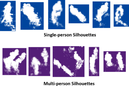
Figure 4: Sample images from the training dataset used for machine learning and image classification.

3.7 Privacy Enhancement

In our system, the videos and images are discarded immediately after processing. Still, privacy invasion is always a concern for video based detection methods. With this in mind, we introduced a number of techniques to preserve the privacy of the occupants. First of all, to prevent any potential hacker from accessing the video feed, we ensured that the camera stream can only be accessed by a single process at a time. Consequently, when our system is running, all the other programs are blocked from accessing the camera. In addition, a hardware-based solution has been tested. Specifically, we created a frosted lens by overlaying a semi-transparent layer in front of the camera, so as to blur the camera feed. In so doing, the faces of occupants are no longer recognizable; see Figure 5 for an illustration.

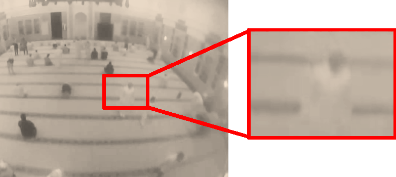
Figure 5: Enhanced privacy by using frosted lens on camera.

3.8 Evaluation Results

In this section, we evaluate the accuracy of our occupancy recognition. To this end, we collected video footages from our testbed, each with a frame size of 800$\times$600 pixels, and a sample rate of 30 frames per second. The true occupancy was obtained by manually counting the number of occupants in each frame. Due to this laborious process, we were only able to obtain the true occupancy in a small number of videos, which are used in the evaluations.

We start by defining the accuracy rate as follows:

$${\sf AccuracyRate}\triangleq 1-\frac{{\sf Missing}_{\rm in}+{\sf Missing}_{\rm out}}{{\sf Total}_{\rm in}+{\sf Total}_{\rm out}}$$ (1)

where ${\sf Total}_{\rm in}$ is the number of individuals who entered the building and ${\sf Missing}_{\rm in}$ is the number of such individuals who were undetected by the algorithm. Conversely, ${\sf Total}_{\rm out}$ is the number of individuals who exited the building and ${\sf Missing}_{\rm out}$ is the number of those who exited without being detected by our algorithm.

Table 1 presents the system accuracy given different numbers of occupants over different durations. As can be seen, the algorithm is able to recognize the number of occupants with high accuracy, even when over 400 individuals enter the building in just 20 minutes. Naturally, given a greater rate at which occupants enter the building, the accuracy of the system decreases because there are more cases in which the occupants overlap (in many such cases, it was hard, even for a human, to determine the exact number of occupants, and the video had to be replayed several times before the human was able to determine the true occupancy with certainty).

Table 1: Results of occupancy recognition given different durations and different numbers of occupants.

Video Length	Total No. of Occupants	${\sf AccuracyRate}$
	of Occupants
40 mins	127	90%
40 mins	154	90%
20 mins	407	84%

Next, we evaluate our system over one-day periods during the weekend, weekday and Friday. Note that in our testbed Friday is the busiest day in the week due to the Friday sermon, which takes place only once a week, and typically attracts a large audience. The results are presented in Table 2. As expected, the system accuracy correlates with the occupancy rates. In particular, the system is least accurate on Friday (which is the busiest day in our experiment), and most accurate during the weekend (which is the least busy in our experiment). Importantly, the accuracy seems sufficiently high throughout the week to provide a reasonable approximation of the actual occupancy state in the building, which is arguably sufficient for our purpose of HVAC control.

Table 2: Results of occupancy recognition comparing weekend, weekday, and Friday.

Type	Video Length	${\sf AccuracyRate}$
Weekend	1 day	88%
Weekday	1 day	86%
Friday	1 day	81%

We now turn our attention to quantifying the loss in accuracy that occurs when using our privacy-preserving frosted lens from Section 3.7. The results of this evaluation are presented in Table 3. As can be seen, the frosted lens only reduces the accuracy slightly, and that is despite the fact that the video footage is considerably blurred, as we have shown earlier in Figure 5.

Table 3: Results of occupancy recognition comparing normal lens and frosted lens.

Type	Video Length	Total No.	${\sf AccuracyRate}$
		of Occupants
Normal Lens	160 mins	322	87.8%
Frosted Lens	160 mins	339	80.2%

Next, we evaluate the effectiveness of our machine-learning technique from Section 3.6. To this end, we use three performance measures that are widely used in the Machine-Learning literature. The first is ${\sf Precision}$, which is defined as the fraction of occupants that were correctly classified out of all those who were classified as either moving inward or as moving outward. The second measure is ${\sf Recall}$, defined as the fraction of occupants that were correctly classified out of all those who actually entered the building or exited it. Since it is often possible to have a naive classifier that has a high ${\sf Precision}$ but a low ${\sf Recall}$ or vice versa, a better metric called ${\sf F1\mbox{-}Score}$ has been utilized in [44, 45], which is basically a harmonic mean of ${\sf Precision}$ and ${\sf Recall}$. Based on those three measures, Table 4 shows the results before and after applying our machine-learning technique. The evaluation is carried out using 10-fold cross-validation of our dataset of 13,000 blobs. As can be seen, according to the most important measure, namely ${\sf F1\mbox{-}Score}$, our machine-learning technique from Section 3.6 significantly improves the performance of our system.

Finally, to better understand how occupancy changes during the daytime in our application, we plotted in Figure 6 the actual occupancy, as well as the occupancy detected by our algorithm, given a typical Friday, and a typical Saturday. As can be seen, the general occupancy trend is clearly captured by the algorithm.

Table 4: Results of occupancy recognition comparing with and without machine-learning technique.

Type	${\sf Precision}$	${\sf Recall}$	${\sf F1\mbox{-}Score}$
Without Machine Learning	0.97	0.27	0.42
With Machine Learning	0.69	0.78	0.73

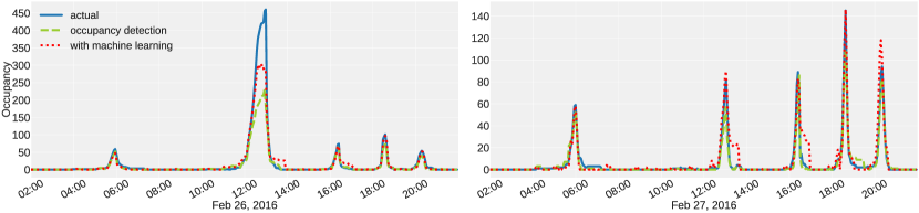
Figure 6: How occupancy changes during a typical day. Each peak represents one of the five daily prayers in Islam. We distinguish between Friday and other days of the week due to the Friday sermon, which precedes the midday prayer and usually attracts many more worshippers compared to any other prayer throughout the week (note that the scale of the y-axis is greater in the left plot than in the right plot).

4 Occupancy Prediction

This section describes our methodology for predicting the future occupancy of the building. Such predictions can be very helpful when optimizing the HVAC control, especially in an application like ours, where occupants arrive in large numbers over short periods of time (see Figure 6). For example, being able to predict the arrival of a large number of people allows the system to pre-cool the building in anticipation of their arrival. Likewise, by predicting that all the occupants will shortly be leaving the building (e.g., if a certain social event was coming to an end), the system can turn off the HVAC system before the occupants even start departing.

In Section4.1 we propose a general-purpose approach to occupancy prediction. After that, in Section 4.2, we further develop our occupancy prediction to produce a domain-specific approach, tailored to our application. Lastly, in Section 4.3 we evaluate our domain-specific prediction by quantifying the impact that it makes on the overall performance of our system.

4.1 General Approach

As a starting point, let us consider a linear regression model, trained using all past occupancy data; let us denoted such an approach by $\widehat{\sf LR}_{\rm AllData}$. To take this simple approach one step further, let us extend the linear regression model by incorporating any “special events” that may cause an abrupt change in the occupancy trend. Any such special event may be recurrent, with a slightly flexible timing and duration. For instance, consider a hall that can be booked in advance for social activities; here every such activity can be thought of as a special event. Information about a special event (such as the average timing and duration, for example) may be available a priori or may be inferred from the past occupancy data. The resulting approach, whereby special events are explicitly modeled, will be denoted by $\widehat{\sf LR}_{\rm SpEv}$, where ${\rm SpEv}$ stands for Special Event. We suggest using this approach with the following linear regression model:

$$\widehat{y}^{(t)}=\beta_{\rm 0}+\beta_{\rm 1}x^{(t)}_{\rm pastEvent}+\beta_{\rm 2}x^{(t)}_{\rm nextEvent}+\beta_{\rm 3}x^{(t)}_{\rm specialCase}$$ (2)

where $\widehat{y}^{(t)}$ is the target variable (i.e., the predicted occupancy at time $t$); $\beta_{\rm i}:i\in\{0,1,2,3\}$ are the parameters of the model; $x^{(t)}_{\rm pastEvent}$ is the difference in time between $t$ and the timing of the past event; and likewise $x^{(t)}_{\rm nextEvent}$ is the difference between $t$ and the timing of the next event; $x^{(t)}_{\rm specialCase}$ is a binary variable that takes a value of 1 if $t$ coincides with a special case and takes a value of 0 otherwise (an example of such a binary variable is $x^{(t)}_{\rm newYearEve}$, which indicates whether $t$ coincides with new year’s eve). Of course, Eq. 2 is only meant as an example of the possible models that one could choose in order to explicitly model the special events that affect the occupancy. One may instead use other features, depending on the application at hand.

4.2 Domain-specific Approach

In this section, we tailor our general-purpose approach from Section 4.1 to our testbed, i.e., the mosque. In this particular application, the special events are the five daily prayers in Islam, the timing of which depends on the position of the sun in the sky. More specifically, the daily prayers are held (1) at dawn; (2) at midday right after the sun passes its highest; (3) at the late part of the afternoon; (4) just after sunset; and (5) between sunset and midnight. As such, the prayer times vary over the course of the year, because days tend to be longer in summer and shorter in winter. Importantly, the “Friday prayer” (which takes place every Friday at midday) is preceded by a sermon, the attendance of which is obligatory for Muslims. As such, the number of occupants increases significantly compared to any other prayer throughout the week.

With this in mind, we now modify the general-purpose approach from Section 4.1 by incorporating our domain-specific knowledge of the application at hand. To this end, we consider (i) the difference in minutes between the current time and the past prayer, (ii) the difference in minutes between the current time and the next prayer, (iii) the current day of the week, and (iv) whether or not it is a public holiday. Then, to predict the occupancy at any given time, $\bar{t}$, we consider historical data for which the timestamp is within a certain threshold from $\bar{t}$. This threshold varies according to time of the year, to reflect the constantly-shifting prayer times. Based on these features, we propose the following linear regression model:

$$\begin{split}\widehat{y}^{(t)}&=\beta_{\rm 0}+\beta_{\rm 1}x^{(t)}_{\rm pastPrayer}+\beta_{\rm 2}x^{(t)}_{\rm nextPrayer}\\ &+\beta_{\rm 3}x^{(t)}_{\rm holiday}+\beta_{\rm 4}x^{(t)}_{\rm dayOfWeek}\end{split}$$ (3)

where $x^{(t)}_{\rm pastPrayer}$ is the difference between $t$ and the timing of the past prayer; $x^{(t)}_{\rm nextPrayer}$ is the difference between $t$ and the timing of the next prayer; $x^{(t)}_{\rm holiday}$ is a binary variable indicating whether or not $t$ coincides with a public holiday; and $x^{(t)}_{\rm dayOfWeek}$ is the day of the week at time $t$. The resulting approach will be denoted by $\widehat{\sf LR}_{\rm DomSp}$, where ${\rm DomSp}$ stands for Domain Specific. In addition to this linear regression model, we also experimented with a polynomial regression model, denoted by $\widehat{\sf PR}_{\rm DomSp}$, which uses the same features as those used in $\widehat{\sf LR}_{\rm DomSp}$.

4.3 Evaluation Results

We use two standard metrics to evaluate the effectiveness of the proposed prediction models: ${\sf R\mbox{-}squared}$ and ${\sf RMSE}$ (Root Mean Squared Error). Both of these metrics are always between 0 and 1. Importantly, with ${\sf R\mbox{-}squared}$ the greater the value the better the model, whereas with ${\sf RMSE}$ the smaller the value the better the model.

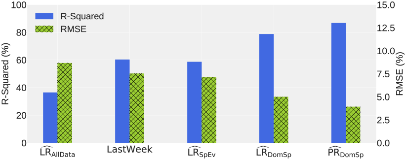
Figure 7: Results of occupancy prediction.

As a baseline model, we use a naive approach, denoted by LastWeek, whereby the current week’s occupancy is assumed to be identical to last week’s occupancy (e.g., the occupancy pattern in, say, the coming Monday is assumed to be identical to that of last Monday). The results are shown in Figure 7, where all models are evaluated with a forecasting horizon of 24-hour ahead. As can be seen, even LastWeek (the most naive approach) outperforms $\widehat{\sf LR}_{\rm AllData}$ (the general-purpose linear regression model trained using all past occupancy data).

In contrast, the performance of $\widehat{\sf LR}_{\rm SpEv}$ (the linear regression model whereby the special events are explicitly modeled) appears to be on par with that of LastWeek. As for the domain-specific approaches, namely $\widehat{\sf LR}_{\rm DomSp}$ and $\widehat{\sf PR}_{\rm DomSp}$, they outperform the other alternatives due to three main reasons: (i) they take into account the day of the week, which is particularly important since the weekly sermon takes place every Friday; (ii) they are able to recognize public holidays, during which the occupancy typically increases in residential areas and decreases in commercial areas; (iii) they are trained using data from only the past 30 days (as opposed to using all past occupancy data), which is important since the prayer times are constantly shifting throughout the year; this shift is usually negligible over a 30-day period, but can be significant over the course of a year. Perhaps not surprisingly, between the two domain-specific approaches, $\widehat{\sf PR}_{\rm DomSp}$ outperforms $\widehat{\sf LR}_{\rm DomSp}$. Based on this evaluation, we adopt $\widehat{\sf PR}_{\rm DomSp}$ as our model of choice. With an R-squared value of about 0.87 and an RMSE value of about 0.03, this model appears to capture the overall occupancy trend to a satisfactory degree for the purpose of HVAC control.

5 Building Thermal Response Simulation

Traditional building modeling and control is often based on simplified mathematical building models due to their tractability and ease of use. However, these simplified models (e.g., first-principle linear models) can capture only limited aspects of the dynamic nature of buildings and systems. On the contrary, sophisticated building simulation software can use more realistic physical models, which in turn provide accurate modeling of the thermal behavior of buildings. One prominent example is EnergyPlus, a popular building energy simulation program that can create detailed building envelope and system models. EnergyPlus can perform extensive conductivity analyses, and can even consider local weather conditions, by either incorporating user-supplied information or by using EnergyPlus Weather Files [46]. Furthermore, it provides interfaces with which external tools and programs can inter-operate. This process is known as co-simulation, whereby different subsystems are integrated to carry out the simulation and calibration process simultaneously. With co-simulation, multiple simulators and software tools can be coupled in such a way that the strengths of each tool are exploited while overcoming their individual weaknesses. Currently, EnergyPlus is commonly used for planning and energy auditing. Using EnergyPlus for real-time HVAC control presents both opportunities and challenges. In this section, we utilize a framework of co-simulation in order to adapt EnergyPlus for real-world HVAC control.

5.1 Basic Building Geometry

First, the basic geometry of the building is created for EnergyPlus. In our testbed, we consider the large indoor space of a mosque installed with packaged rooftop HVAC units with ceiling-based cool air distribution. The detailed descriptions of the testbed, including dimensions and HVAC system specifications are provided in Table 5.

Table 5: Description of the testbed building.

Dimensions	18m$\times$18m$\times$7m
Walls	Outer Layer	Stucco
	Middle Layer	Concrete
	Inner Layer	Gypsum
Doors	Wood Stile and Rail
Windows	Glass with Vinyl Framing
Packaged Rooftop HVAC	Cooling Capacity	175840W
	Air Flow Rate	7.56m3/sec

We employ SketchUp for 3D modeling with the default material properties for walls, windows, and doors. Then, the 3D model is imported to OpenStudio, where the parameters of the HVAC system are incorporated into the model, based on the vendor’s specifications and datasheet. The SketchUp building model and the corresponding OpenStudio model are visualized in Figure 8. Apart from the basic geometry and properties of the building, many parameters still need to be calibrated according to the available data; this will be the focus on the next subsection.

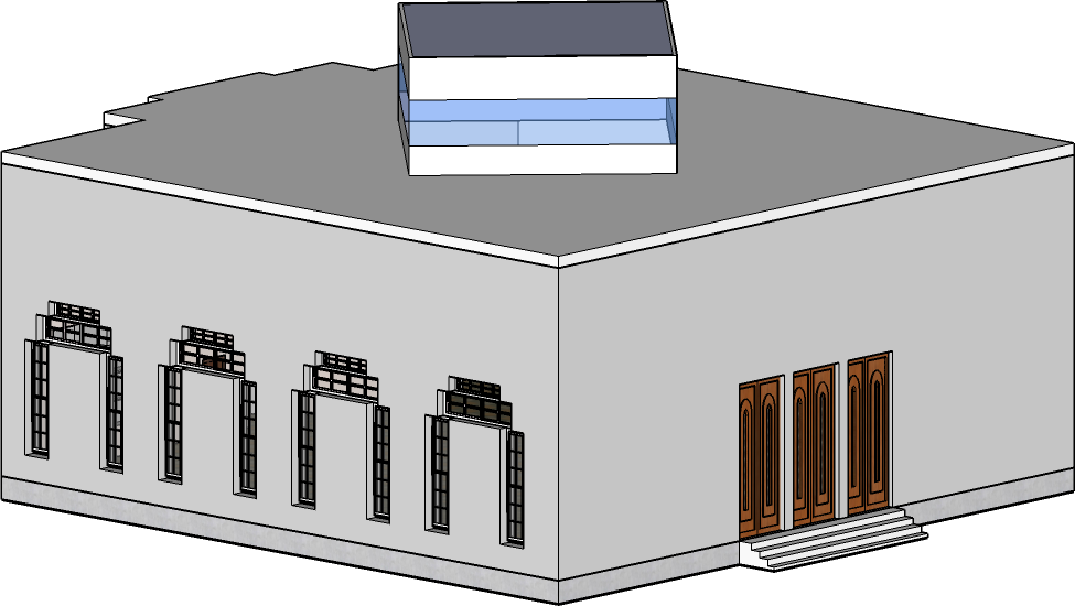
(a)

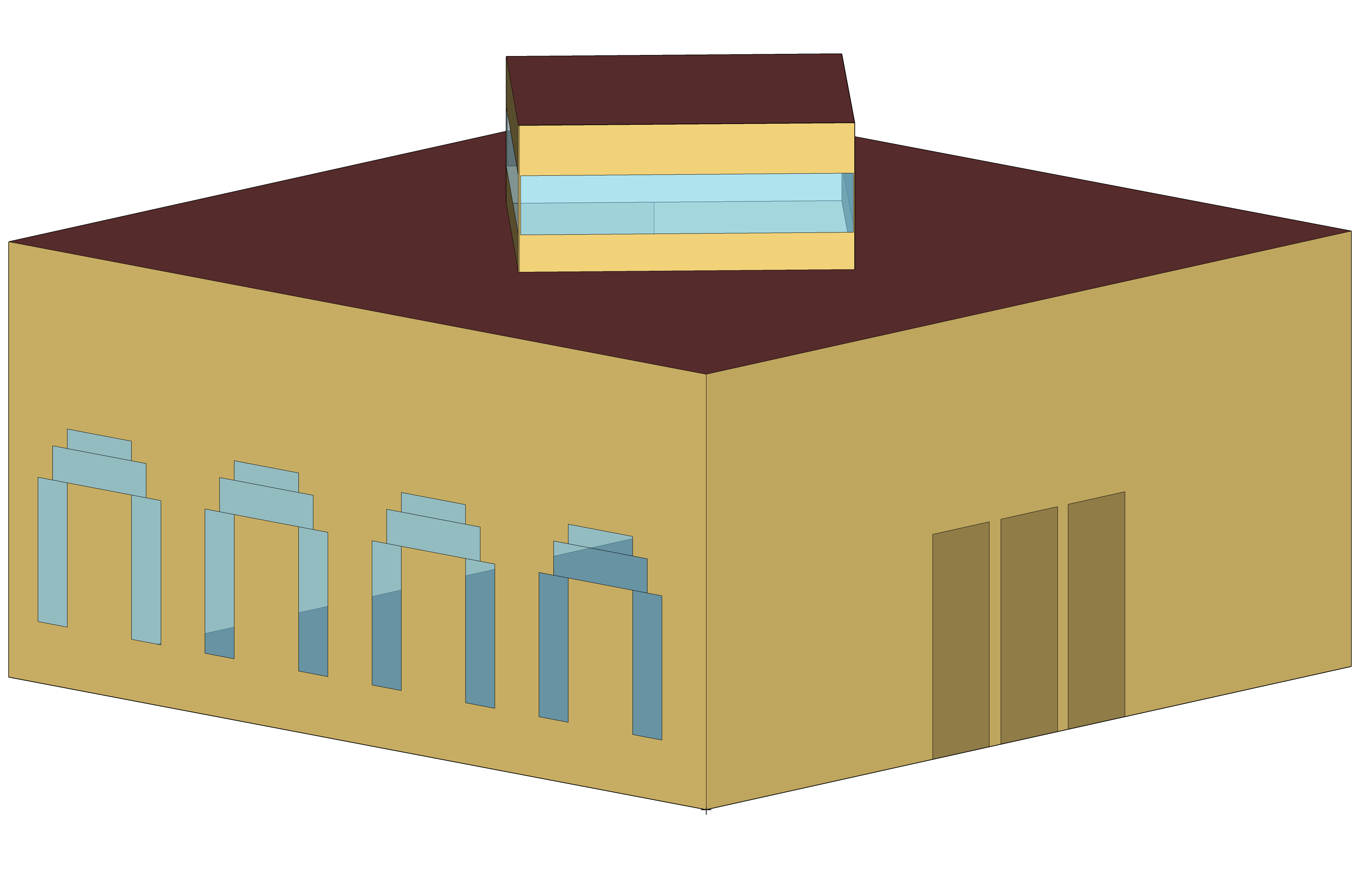
(b)

Figure 8: Basic building models. (a) 3D SketchUp building model, (b) the corresponding OpenStudio model.

5.2 Building Model Calibration

To obtain an accurate simulation of the thermal response of the building, we must first calibrate the parameters of the building model so as to minimize the gap between the simulated indoor temperature and the measured one. To this end, we use an inverse calibration approach, whereby the model’s outputs are used to calibrate the parameters of the model. This calibration process is carried out using the co-simulation framework illustrated in Figure 9. In particular, the framework couples the EnergyPlus building model with our calibration algorithm which we implemented using Python; this coupling is done using the BCVTB (Building Controls Virtual Test Bed) software tool [47], which provides a data-exchange interface between EnergyPlus and Python. Moreover, BCVTB allows EnergyPlus to take into consideration the real-world data measured from our testbed, such as observed occupancy and temperature.

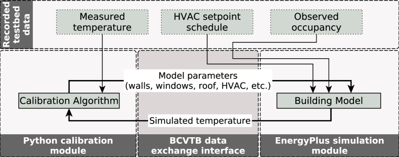
Figure 9: Co-simulation framework using BCVTB.

Out of the numerous parameters that can be calibrated in EnergyPlus, we focus on a particular set of uncertain parameters as our candidates for calibration, because they are either unknown or likely to deviate from the datasheet. Specifically, these parameters are the cooling capacity and air flow rate of the HVAC system, as well as the thickness and conductivity of the roof, the walls, and the windows.

Now, we will explain how the calibration process is done. To this end, we use a dedicated algorithm, the flowchart of which is depicted in Figure 10. The algorithm is based on the notion of gradient descent, where values of those parameters are updated iteratively until the error between the simulated indoor temperature and the measured temperature is within an acceptable threshold. Next, we explain each step of this algorithm.

Figure 10: Flowchart of the model-calibration algorithm.

Let $X=\{x_{1},x_{2},\dots,x_{K}\}$ denote the set of parameters to be calibrated. For every $x_{k}\in X$, the algorithm runs a series of $N$ co-simulations, updating the model in every iteration using a different value of $x_{k}$ while keeping the values of the remaining parameters unchanged. Specifically, in the $i^{\textnormal{th}}$ iteration of this process (where $i\in\{1,\ldots,N\}$) the error is calculated as the difference between the measured temperature and the simulated model temperature; this error is denoted by:

$$\varepsilon(x_{1},\ldots,x_{k-1},x_{k}^{i},x_{k+1},\ldots,x_{K})$$

where $x_{k}^{i}$ takes the value of $x_{k}$ in the $i^{\textnormal{th}}$ iteration. For notational convenience, let us write $(x^{i}_{k},x_{-k})$ instead of writing $(x_{1},\ldots,x_{k-1},x^{i}_{k},x_{k+1},\ldots,x_{K})$. Then the optimal value for $x_{k}$, denoted by $x^{*}_{k}$, can be computed as follows:

$$x^{*}_{k}=\underset{i=1,\dots,N}{\arg\min}\ \ \varepsilon(x^{i}_{k},x_{-k})$$ (4)

After computing $x^{*}_{k}$ for every $k\in\{1,\ldots,K\}$, the algorithm checks whether $\varepsilon(x^{*}_{1},x^{*}_{2},\dots,x^{*}_{K})$ is within the acceptable threshold. If so, then it outputs $(x^{*}_{1},x^{*}_{2},\dots,x^{*}_{K})$ and terminates; otherwise it repeats the entire process but after updating the parameters, i.e., after setting $x_{k}\leftarrow x^{*}_{k}$ for every $k\in\{1,\ldots,K\}$. We note that the outcome of the calibration process is not affected by the order in which the algorithm iterates over the parameters.

5.3 Evaluating the Model-Calibration Algorithm

To evaluate the algorithm from Figure 10, we use two standard metrics, namely: the Coefficient of Variation of Root Mean Squared Error (${\sf CVRMSE}$) and the Mean Bias Error (${\sf MBE}$); these are computed as follows:

$${\sf CVRMSE}=\frac{\sqrt{\sum_{t=1}^{M}\left[\frac{(T_{\rm t}-\hat{T}_{\rm t})^{2}}{M}\right]}}{\frac{1}{M}\sum_{t=1}^{M}T_{\rm t}}$$ (5)

$${\sf MBE}=\frac{\sum_{t=1}^{M}(T_{\rm t}-\hat{T}_{\rm t})}{\sum_{t=1}^{M}T_{\rm t}}$$ (6)

where ${T_{\rm t}}$ and ${\hat{T}_{\rm t}}$ are the measured and simulated temperature values at time $t$, respectively, and $M$ is the total number of simulation time steps. Both MBE and CVRMSE provide different insights to the calibration process. However, the CVRMSE is arguably superior because unlike MBE it does not suffer from the cancellation effect [48].

Table 6: Parameters used for model calibration.

Parameter	Field		Initial Value	Calibrated Value
	Outer Layer	Thickness	2.53cm	7.72cm
	(Stucco)	Conductivity	0.69W/(m-K)	0.16W/(m-K)
Exterior	Layer 2	Thickness	20.32cm	62.01cm
Walls	(Concrete)	Conductivity	1.31W/(m-K)	0.311W/(m-K)
	Layer 3	Thickness	1.27cm	3.87cm
	(Gypsum)	Conductivity	0.16W/(m-K)	0.037W/(m-K)
HVAC	Cooling Capacity		87920W	164850W
	Air Flow Rate		3.78m3/sec	7.08m3/sec

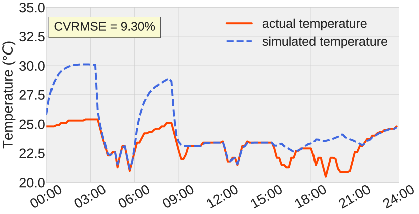
(a) Using the default parameter values set by SketchUp during initial model creation.

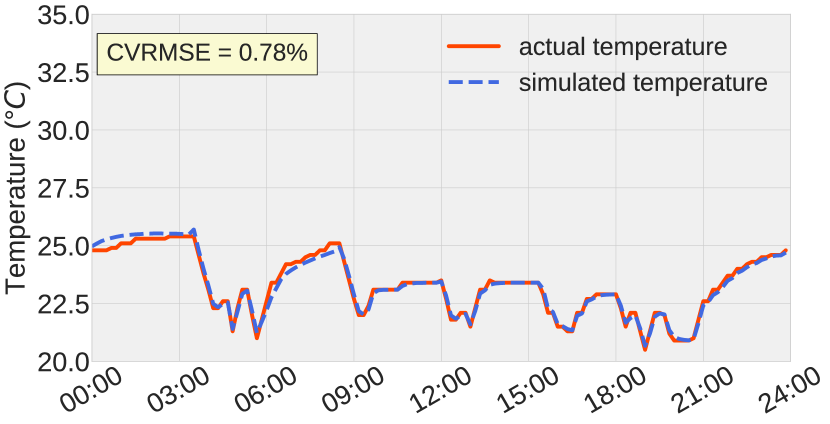
(b) Using the calibrated parameter values from our model-calibration algorithm.

Figure 11: Results of model calibration.

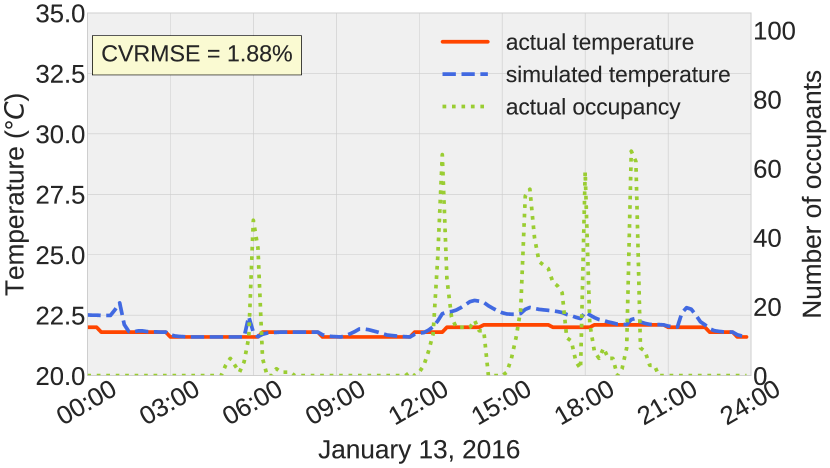
(a) A typical day in winter with AC turned off.

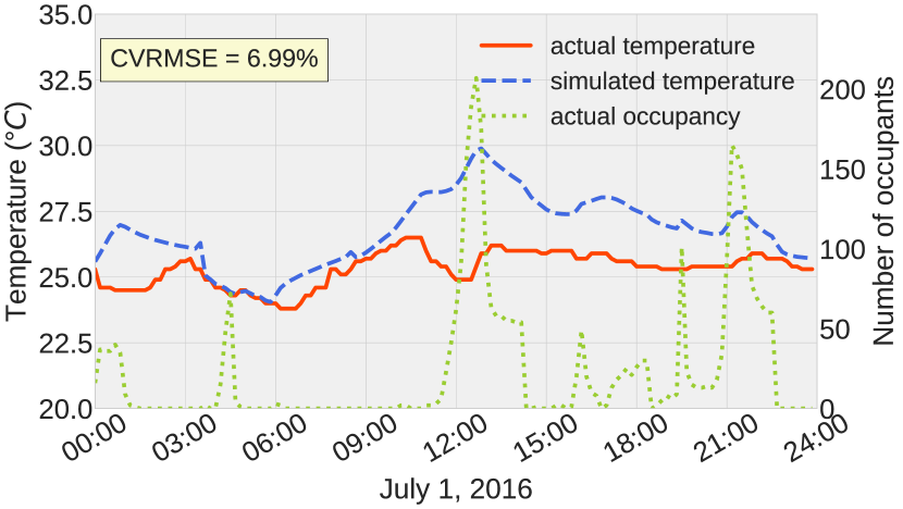
(b) A hot day in summer.

Figure 12: Results of testing calibrated model with validation sets.

The default and calibrated values of our model parameters are listed in Table 6. Note that we don not manually specify the allowed parameter ranges. EnergyPlus performs automatic parameter range checking using Input Data Dictionary [49], which specifies the maximum and/or minimum values of parameters.

Using a simulation period of 24 hours, we tested the temperature response of our model before and after the calibration process (we used 24 hours since it is adequate for our purpose of HVAC control). Specifically, the calibration process takes around 100 co-simulations on average, each of which uses sub-hourly data with a sampling time period of 10 minutes. A CVRMSE of less than 2.0% was treated as an acceptable calibration threshold. The results are depicted in Figure 11. In particular, Figure 11(a) plots the actual temperature as well as the simulated temperature, given the default parameter values from SketchUp. In Figure 11(b), the default parameter values are replaced by the ones calibrated using our algorithm from Section 5.2. As can be seen, the simulated temperature of the calibrated EnergyPlus model closely matches the measured temperature. Quantifying the performance gains using the aforementioned metrics, we find that the algorithm achieves MBE$<$1% and CVRMSE$<$1%. This seems satisfactory, bearing in mind that the ASHRAE guidelines, which require that MBE$<$10% and CVRMSE$<$30% for hourly data, and MBE$<$5% and CVRMSE$<$15% for monthly data [50]. We tested our calibrated model with 24-hour periods taken from different times of the year to cover hot and cold days. The results are shown in Figure 12. In particular, Figure 12(a) shows the temperature response of the model on a typical winter day when the HVAC system is turned off. It can be seen that CVRMSE is still below the 2.0% threshold and the model is considered calibrated. Figure 12(b) shows the model response on a hot summer day. In this case, CVRMSE has become above the threshold and the algorithm will need to re-calibrate the model to once again make CVRMSE below the threshold. These figures also show the detected occupancy to demonstrate how the model response varies with changing occupancy patterns. We note that in our testbed building there are no days without occupancy because there are always multiple prayers and multiple worshipers every day.

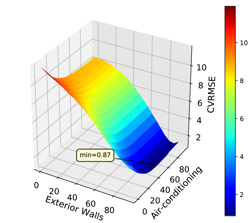
(a)

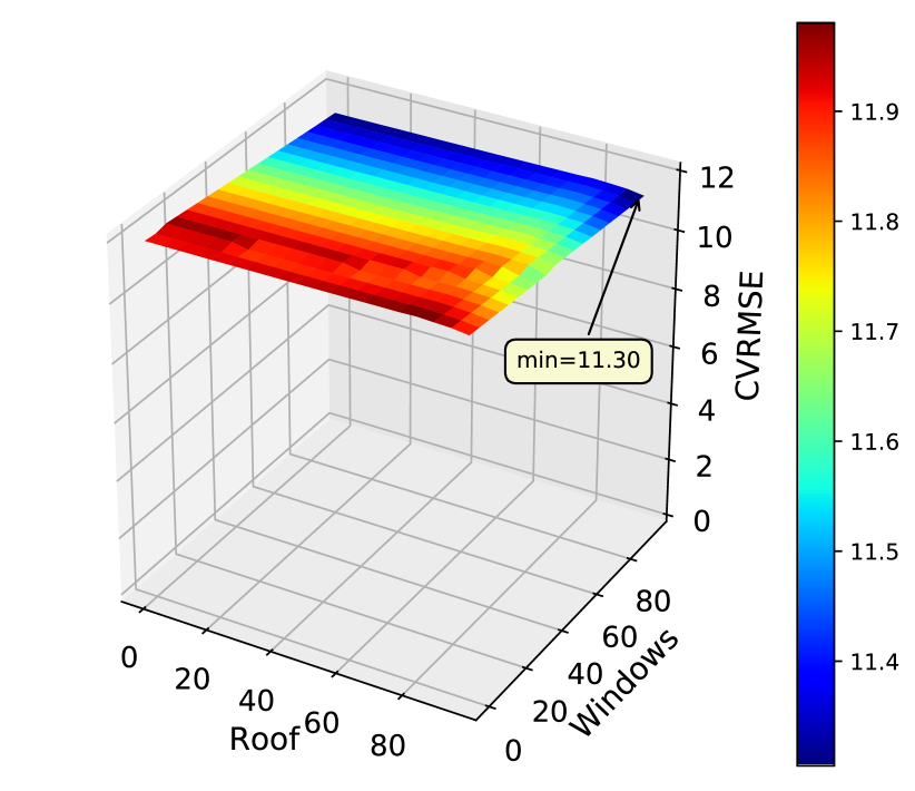
(b)

Figure 13: Examples of how the performance improvements from the calibration process can vary significantly depending on the parameters being calibrated.

We observe that the calibrated values of the uncertain HVAC parameters are very close to the manufacturer’s specifications. In other words, even if those specifications were not available, our approach can still be applied without any noticeable change in performance. This makes our approach more practical in situations where such information is not available. We experimented with parameters other than those outlined in Table 6, and found that their calibration did not yield any noticeable improvements. An example is illustrated in Figure 13. In particular, Figure 13(a) depicts the impact of calibrating two parameters from Table 6, whereas Figure 13(b) depicts the impact of calibrating two parameters that are not outlined in Table 6, which are: (i) the roof’s thickness and conductivity, and (ii) the windows’ thickness and conductivity. Here, the x-axis and y-axis represent the relative change (compared to the default value) in the first parameter and in the second parameter, respectively, while the z-axis represents the corresponding CVRMSE value. As can be seen, the performance improvements from the calibration process vary significantly depending on the parameters being calibrated.

Finally, commenting on the runtime of the calibration algorithm, our implementation on Raspberry Pi 3 took an average of 43 seconds per co-simulation, which allows for about 2000 co-simulations per day (recall that our satisfactory results from Figure 11 required only 100 co-simulations). These results demonstrate that our calibration methodology can be used in practice, to automatically and continuously correct the building model for effective real-time HVAC control using low-cost embedded computers such as Raspberry Pi.

6 Simulation-guided Model Predictive Control

Building upon our occupancy-prediction from Section 4 and our temperature-response simulation from Section 5, we now propose a model predictive control algorithm in Section 6.1, and evaluate it in a real-world HVAC system in Section 6.2.

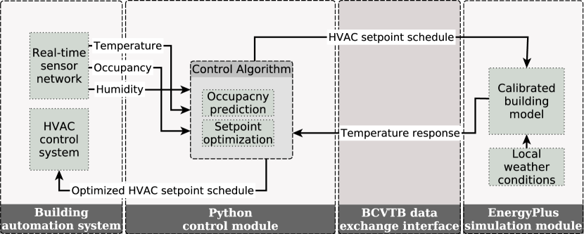
Figure 14: Framework of model predictive control algorithm.

6.1 HVAC Control Framework

The framework of our model predictive control consists of several parts that interact with one another as illustrated in Figure 14. Here, a control algorithm provides an HVAC setpoint schedule to the EnergyPlus simulator through the BCVTB interface. Based on this schedule and the local weather information, the EnergyPlus simulator performs simulations and provides temperature response to the control algorithm. Note that the local weather information is provided by the EnergyPlus Weather File [46] which includes temperature, humidity, pressure, wind speed, solar radiation, luminance, precipitation etc. Now, based on the temperature response as well as the occupancy prediction, the control algorithm checks whether thermal-comfort criteria will be satisfied; if so, then there is no need for any modifications to the HVAC setpoint schedule; if not, then the HVAC setpoint schedule is modified subject to the thermal-comfort threshold, before being sent again to the EnergyPlus simulator, and so on. Once the HVAC setpoint schedule is finalized, the HVAC system starts following this schedule, and the control algorithm starts monitoring the real-time temperature, humidity, and occupancy data, to determine the actual thermal comfort that resulted from its control decisions, and adjust its thermal-comfort threshold accordingly.

Input: $t_{\rm now}$, Initialization: $\tau\leftarrow 0,{\rm timer}\leftarrow 0$

1  if ${\sf occup}_{\rm now}=0\ and\ {\rm timer}=0$ then

2    $T_{\rm target}\leftarrow{\sf setpoint}_{\rm uo}$

3   Set HVAC setpoint to $T_{\rm target}$

4     $\triangleright$ increase setpoint

5    $\tau\leftarrow\emph{Pre-cooling}(t_{\rm now},t_{\rm pd\_oc})$

6     $\triangleright$ pre-cooling time

7    ${\rm timer}\leftarrow t_{\rm now}+\tau$

8 end if

9if $t_{\rm now}={\rm timer}$ then

10    $T_{\rm target}\leftarrow{\sf setpoint}_{\rm oc}$

11   Set HVAC setpoint to $T_{\rm target}$

12     $\triangleright$ start pre-cooling

13    ${\rm timer}\leftarrow\ 0$

14else

15    Wait for timer expiry

16     $\triangleright$ no pre-cooling yet

17   

18 end if

Algorithm 1 HVAC-MPC

Having provided an overview of our framework for model predictive control, we will now explain the control algorithm therein. In particular, we call this algorithm HVAC-MPC, the pseudocode of which is outlined in Algorithm 1. First, in line 1 the algorithm checks whether the building is unoccupied at the current time. If so, then in lines 2 and 3 it instructs the HVAC system to increase the temperature setpoint (see Table 7 for the exact setpoints used by the algorithm).

Table 7: Setpoints used by HVAC-MPC. Here, ${\sf setpoint}_{\rm oc}$ is used when the building is occupied; ${\sf setpoint}_{\rm uo}$ is used when unoccupied.

Occupied (${\sf setpoint}_{\rm oc}$)	Unoccupied (${\sf setpoint}_{\rm uo}$)
24∘C	28∘C

After that, in lines 4 and 5, the occupancy prediction is used to determine when the building is expected to become occupied in the future, and determine the optimal pre-cooling time accordingly (here the algorithm uses a procedure called Pre-cooling, the workings of which will be explained later on in this section). Then, in line 7, the algorithm checks whether the time has come for the pre-cooling to start. If so, then it instructs the HVAC system to decrease the temperature setpoint, before resetting the corresponding timer (see lines 8 to 10). On the other hand, if the time has not yet come to start pre-cooling, the algorithm simply waits until it does (see lines 11 and 12).

Figure 15: Flowchart of our Pre-cooling procedure, which determines the pre-cooling time based on the predicted occupancy.

Having explained the pseudocode of HVAC-MPC, we now explain the workings of the Pre-cooling procedure used therein. Figure 15 illustrates the flowchart of this procedure. Basically, the goal here is to determine the time $t^{*}$ at which the pre-cooling should start; this time falls within a certain range of feasible times, denoted by $[t_{\rm min},t_{\rm max}]$. Initially, the algorithm sets $t_{\rm min}$ to be equal to the current time (i.e., $t_{\rm now}$), sets $t_{\rm max}$ to be equal to the predicted time of occupancy (i.e., $t_{\rm pd\_oc}$), and sets $t^{*}$ to be right in the middle between the two (i.e., $t^{*}=t_{\rm min}+(t_{\rm max}-t_{\rm min})/2$). After that, $t^{*}$ is adjusted iteratively as follows. In each iteration, the algorithm runs an EnergyPlus simulation in which the HVAC is switched off from $t_{\rm min}$ to $t^{*}-1$, and then the pre-cooling starts at $t^{*}$, leaving the HVAC on from $t^{*}$ to $t_{\rm max}$. Thus, we obtain the simulated temperature, $T_{\rm sim}[t]$, for every $t\in[t_{\rm min},t_{\rm max}]$. These simulated temperatures should ideally satisfy the following conditions:

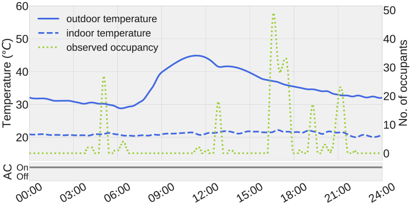
(a) Without HVAC-MPC: full-powered HVAC at all times (indicated by the strip at the bottom) despite intermittent occupancy.

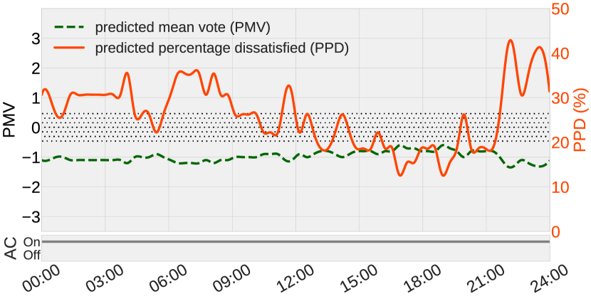
(b) Without HVAC-MPC: incurred thermal comfort sensation. PMV index is always outside the recommended [-0.5,+0.5] range.

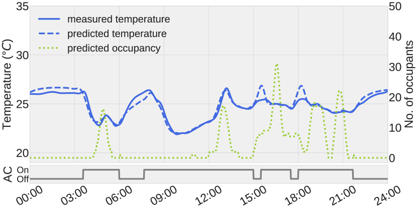
(c) With HVAC-MPC: occupancy and temperature forecasts are used to find the best possible pre-cooling schedule as indicated by the sequence of HVAC state transitions from off to on in the strip at the bottom.

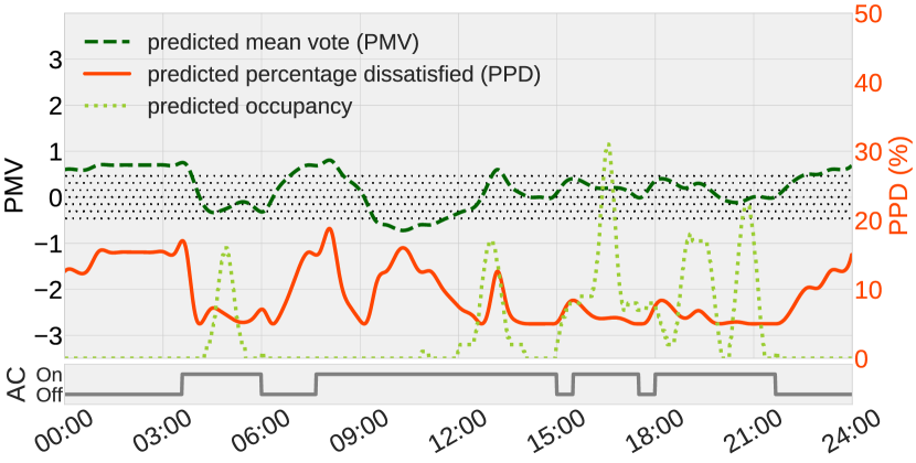
(d) With HVAC-MPC: The PMV index is almost always within the recommended [-0.5,+0.5] range during the periods in which the building is occupied.

Figure 16: Results of HVAC model predictive control (HVAC-MPC) in our testbed.

$$T_{\rm sim}[t_{\rm pd\_oc}]={\sf setpoint}_{\rm oc}$$ (7)

$$T_{\rm sim}[t]>{\sf setpoint}_{\rm oc},\ \forall t:t^{*}\leq t<t_{\rm pd\_oc}$$ (8)

which basically means that the temperature becomes satisfactory exactly when needed, and not before. The algorithm checks whether the above two conditions hold. Now:

• if Condition (7) does not hold, it implies that the pre-cooling process started too late, and so $t^{*}$ should be set to an earlier time. To this end, the algorithm sets $t_{\rm max}$ to be equal to $t^{*}-1$, and then updates $t^{*}$ as follows:

  $$t^{*}\leftarrow t_{\rm min}+(t^{*}-t_{\rm min})/2$$ (9)

• if Condition (8) does not hold, it implies that the pre-cooling process started too soon, and so $t^{*}$ should be delayed. To this end, the algorithm sets $t_{\rm min}$ to be equal to $t^{*}+1$, and then updates $t^{*}$ as follows:

  $$t^{*}\leftarrow t^{*}+(t_{\rm max}-t^{*})/2$$ (10)

After that, the algorithm proceeds to the next iteration to check whether the new $t^{*}$ needs any further adjustments. This process is repeated until either $t_{\rm min}\geq t_{\rm max}$, or conditions (7) and (8) are both met. Either way, the best possible $t^{*}$ is found.

6.2 Evaluation Results

In this subsection, we evaluate the performance of our HVAC-MPC algorithm. To this end, we consider two standard measures of thermal comfort, namely Predicted Mean Vote (PMV) and Predicted Percentage Dissatisfied (PPD) [51]. Specifically, PMV quantifies the human perception of thermal sensation on a scale that runs from -3 to +3, where -3 is very cold, 0 is neutral, and +3 is very hot. On the other hand, PPD is built upon PMV to quantify the percentage of occupants that are dissatisfied given the current thermal conditions. The recommended PMV range for thermal comfort is between -0.5 and +0.5 for indoor spaces, while the acceptable PPD range is between 5% and 10% [52].

We compared our HVAC-MPC algorithm against a baseline alternative, where the HVAC is turned on throughout the day, regardless of the varying occupancy. The evaluation results are shown in Figure 16. Specifically:

• Figure 16(a) depicts the observed occupancy, the indoor and outdoor temperatures, and the HVAC status given the baseline HVAC control;

• Figure 16(b) depicts the thermal comfort according to PMV and PPD given the baseline HVAC control;

• Figure 16(c) depicts the predicted occupancy, the indoor temperature, and the HVAC status given HVAC-MPC algorithm;

• Figure 16(d) depicts the thermal comfort according to PMV and PPD given HVAC-MPC algorithm.

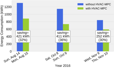
(a) When compared to the immediately preceding day.

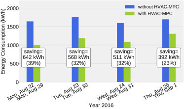
(b) When compared to the same day of the preceding week.

Figure 17: Reduction in HVAC energy consumption achieved by HVAC-MPC (Algorithm 1).

Let us first comment on the results of the baseline HVAC control. As can be seen in Figure 16(a), the HVAC is turned on throughout the day, despite the significant changes in both the occupancy and the external temperature. In terms of thermal comfort, the baseline HVAC control performs rather poorly, as shown in Figure 16(b). Here, the recommended range for PMV is highlighted by the dotted region. As can be seen, the PMV index is outside the recommended range throughout the day. Furthermore, according to the PDD index, a considerable percentage of occupants are dissatisfied most of the day.

Moving on to the results of our HVAC-MPC algorithm, Figure 16(c) shows how the HVAC is switched off for a considerable number of hours. This is because, whenever the building becomes unoccupied, HVAC-MPC increases the temperature setpoint and predicts the future temperature and occupancy to find the best possible time for pre-cooling. Figure 16(d), on the other hand, depicts the PMV and PPD indices throughout the day. As can be seen, when the building is occupied, the PMV index is almost always within the recommended range. Likewise, when the building is occupied, the PPD is close to 5% (which is the best possible PPD score that can be achieved).

Finally, we present the energy savings that are attained by our HVAC-MPC algorithm. The algorithm was activated in the testbed building for a duration of one week in total and the results are provided in Figure 17. In particular, Figure 17(a) shows the results for three different days, where each day is in a different month. For each day shown, the algorithm performance is compared with the immediately preceding day where HVAC-MPC is not activated. Figure 17(b) shows the results of another experiment where we activated HVAC-MPC for four consecutive days in the same week. For each day, the results are compared with the corresponding day of the previous week in which HVAC-MPC was not activated. The purpose of this experiment was to find out how much energy is saved by the MPC algorithm relative to the same day of the previous week. The energy savings attained by HVAC-MPC range from 23% to 39%. Table 8 lists the average daily savings, the standard deviation, and the total energy savings over the experiment period.

Table 8: Summary of energy savings attained by HVAC-MPC.

Average daily savings over experiment period	456 kWh
Standard deviation of daily savings	118 kWh
Total savings over the seven-day experiment	3197 kWh

7 Testbed Design and Implementation

Our automatic HVAC control system with real-time video-based occupancy recognition and EnergyPlus-guided model predictive control is implemented on the Raspberry Pi 3 platform. Our choice is motivated by the fact that Raspberry Pi 3 is a low-cost embedded system platform that costs as little as $35 per unit, as of 2016. Although there are other embedded systems (e.g., Intel Galileo), to the best of our knowledge, Raspberry Pi is the cheapest in the market for our purpose of HVAC control. A comparison of different embedded systems in terms of cost and performance can be found in [53]. Another advantage of Raspberry Pi 3 is its rich set of specifications, which include: 1.2GHz 64-bit quad-core CPU, 1GB SDRAM memory, SD card based expandable external data storage, WiFi & Bluetooth connectivity, and GPU. The remainder of this section provides more details about our testbed design and implementation.

7.1 System Design

Figure 18 illustrates the overall design of our system. This system is comprised of two subsystems: (1) the building automation system, and (2) the cloud-based management system. Next, we explain each of these systems.

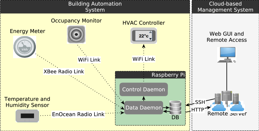
Figure 18: Outline of our system, which is comprised of two subsystems: (1) the building automation system, and (2) the cloud-based management system.

Starting with the building automation system, it consists of the hardware components installed in the building, including temperature and humidity sensors, occupancy monitors, energy meters, and customized wireless HVAC controllers. The temperature and humidity sensors are based on EnOcean technology, and have the advantage of being self-powered and maintenance-free, which makes them highly flexible for deployment anywhere in the target environment. The occupancy monitor consists of a dedicated Raspberry Pi and a fish-eye camera for real-time tracking of occupancy. An Arduino-based energy meter is used to measure the energy consumption of the HVAC units. A data daemon running on the base station Raspberry Pi stores the data received from these components. The data daemon also provides the received data to a control daemon (also running on the base station Raspberry Pi), which uses it to make HVAC control decisions. To this end, the control daemon interfaces with the HVAC system through wireless controllers implemented in a Raspberry Pi. The base station module is shown in Figure 19(d).

Having described the building automation system, we now move on to the cloud-based management system. In particular, this system is comprised of the remote server and the web graphical user interface (GUI). The remote server receives the collected data and stores it in a server database for later analysis and permanent storage. The web GUI retrieves data from the server database for visualization and analysis. The web GUI also provides remote access to the building control system. Secure Shell (SSH) protocol is used as the underlying protocol to securely provide remote access.

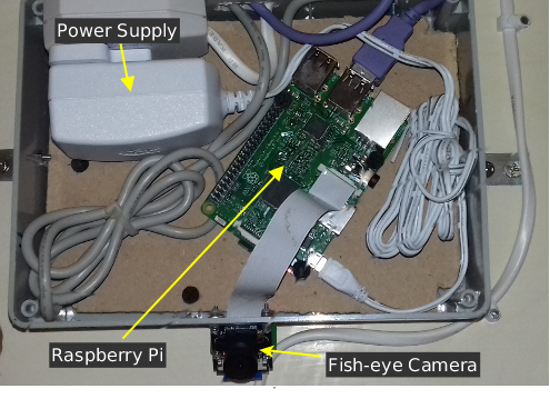
(a)

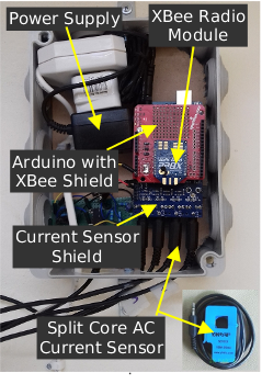
(b)

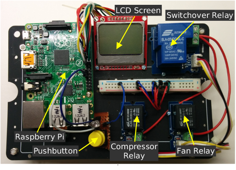
(c)

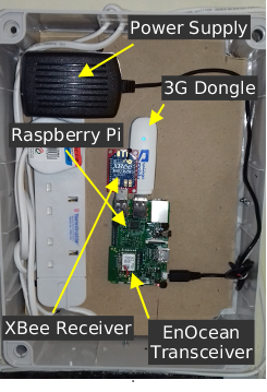
(d)

Figure 19: Testbed system components: (a) occupancy detection module, (b) HVAC energy measurement module, (c) HVAC controller, (d) base station module.

7.2 Occupancy Detection Module

Our system monitors the building occupancy using a Raspberry Pi with a fish-eye camera. In order to keep track of the number of occupants in the building, a video processing algorithm runs on the Raspberry Pi to analyze the real-time video stream captured by the fish-eye camera. Figure 19(a) shows the occupancy module developed for this research. The module should be installed above the building entrance door so that it can monitor the occupancy inside the building. Multiple modules may be needed if the building has multiple entry/exit points, such that each module covers a single point.

7.3 HVAC Energy Measurement Module

To collect the HVAC energy consumption data, we developed an Arduino-based module shown in Figure 19(b). The module design is adapted from the OpenEnergyMonitor framework, which is an open source project for developing energy monitoring and analysis tools [54]. The module uses non-invasive alternating current (AC) sensors to measure the HVAC energy consumption. These sensors can be clipped onto either the live or ground wire coming into the HVAC unit without needing to strip the wire, thus avoiding any high-voltage work. We used a dedicated sensor for each HVAC unit installed in the building. The collected data is sent to the base station through an XBee radio link. It was decided to use XBee radio technology because the HVAC unit power supply can be in a separate room or even on the roof. In such cases, the XBee modules with their extended transmission range can penetrate concrete walls and roofs and are able to transmit the sensor readings to the base station.

7.4 HVAC Controller

Figure 19(c) shows the wireless HVAC controller implemented in Raspberry Pi. The module operates the HVAC unit according to the setpoint schedule, which is determined by the MPC algorithm. The module has three relays, two of which are used to open and close the compressor and fan circuits of the HVAC unit to keep the indoor temperature within fixed bound of the MPC setpoint. The third relay (labeled as Switchover Relay in Figure 19(c)) is used to switch control between our wireless controller and the default HVAC thermostat controller, allowing the building occupants to disable the automatic HVAC control if they are dissatisfied with the current thermal comfort level or if the system is malfunctioning. The module is also equipped with an LCD display to provide status information. By adjusting the setpoints, we actually control the HVAC system directly. This generic approach can be applied to different HVAC systems, with varying specifications.

8 Conclusion

This paper presents an automatic HVAC control system, featuring real-time occupancy recognition, dynamic occupancy prediction, and simulation-guided model predictive control, implemented in a low-cost embedded system (Raspberry Pi). We deployed and evaluated our system for providing automatic HVAC control in the large public indoor space of a mosque. Our experiments showed that our real-time occupancy recognition system can reach 90% accuracy, whereas our occupancy prediction system can reach 85% accuracy. We employ real-time HVAC control guided by an on-board EnergyPlus simulator, which is able to achieve more than 30% energy saving while maintaining the comfort level within acceptable range. Importantly, our system is sufficiently general and can be deployed in other types of buildings with large public indoor spaces.

Notably, we ported the EnergyPlus simulator to the Raspberry Pi embedded system platform. We release our Raspberry Pi version of EnergyPlus publicly [15] to enable other researchers to take advantage of our work for future building automation projects.

Our testbed has been evaluated in buildings with somewhat predictable occupancy patterns. It is challenging to apply our system to settings with irregular occupancy patterns. In future work, we will explore robust online HVAC control using minimal occupancy prediction. Augmented reality is also being integrated in HVAC control system [55]. Online algorithms have been applied to wireless sensor based building control [56, 57]. Robust online control can ensure good performance in the presence of dynamic irregular environmental factors.

References

- [1] L. Pérez-Lombard, J. Ortiz, C. Pout, A review on buildings energy consumption information, Energy and Buildings 40 (3) (2008) 394 – 398.
- [2] F. Oldewurtel, A. Parisio, C. N. Jones, D. Gyalistras, M. Gwerder, V. Stauch, B. Lehmann, M. Morari, Use of model predictive control and weather forecasts for energy efficient building climate control, Energy and Buildings 45 (2012) 15 – 27.
- [3] J. Álvarez, J. Redondo, E. Camponogara, J. Normey-Rico, M. Berenguel, P. Ortigosa, Optimizing building comfort temperature regulation via model predictive control, Energy and Buildings 57 (2013) 361–372.
- [4] S. Salakij, N. Yu, S. Paolucci, P. Antsaklis, Model-based predictive control for building energy management. i: Energy modeling and optimal control, Energy and Buildings 133 (2016) 345 – 358.
- [5] Y. Kwak, J.-H. Huh, C. Jang, Development of a model predictive control framework through real-time building energy management system data, Applied Energy 155 (2015) 1 – 13.
- [6] P.-D. Moroşan, R. Bourdais, D. Dumur, J. Buisson, Building temperature regulation using a distributed model predictive control, Energy and Buildings 42 (9) (2010) 1445–1452.
- [7] F. Ascione, N. Bianco, C. D. Stasio, G. M. Mauro, G. P. Vanoli, Simulation-based model predictive control by the multi-objective optimization of building energy performance and thermal comfort, Energy and Buildings 111 (2016) 131 – 144.
- [8] H. Park, M. Ruellan, A. Bouvet, E. Monmasson, R. Bennacer, Thermal parameter identification of simplified building model with electric appliance, in: 11th International Conference on Electrical Power Quality and Utilisation, 2011, pp. 1–6.
- [9] R. Bălan, J. Cooper, K.-M. Chao, S. Stan, R. Donca, Parameter identification and model based predictive control of temperature inside a house, Energy and Buildings 43 (2) (2011) 748–758.
- [10] J. Hu, P. Karava, A state-space modeling approach and multi-level optimization algorithm for predictive control of multi-zone buildings with mixed-mode cooling, Building and Environment 80 (2014) 259 – 273.
- [11] C.-H. Jan, 10 years of transistor innovations in system-on-chip (soc) era, in: Solid-State and Integrated Circuit Technology (ICSICT), 2014 12th IEEE International Conference on, IEEE, 2014, pp. 1–4.
- [12] Raspberry pi foundation, available at: https://www.raspberrypi.org. Retrieved on 31-Jan-2017.
- [13] B. Pavlin, G. Pernigotto, F. Cappelletti, P. Bison, R. Vidoni, A. Gasparella, Real-time monitoring of occupants’ thermal comfort through infrared imaging: A preliminary study, Buildings 7 (1) (2017) 10.
- [14] D. B. Crawley, L. K. Lawrie, F. C. Winkelmann, W. Buhl, Y. Huang, C. O. Pedersen, R. K. Strand, R. J. Liesen, D. E. Fisher, M. J. Witte, J. Glazer, Energyplus: creating a new-generation building energy simulation program, Energy and Buildings 33 (4) (2001) 319 – 331, special Issue: {BUILDING} SIMULATION’99.
- [15] Energyplus for raspberry pi, available at: https://github.com/muhaftab/energyplus_rpi. Retrieved on 05-May-2017.
- [16] Number of mosques in u.a.e, available at: https://www.awqaf.gov.ae/Affair.aspx?SectionID=3&RefID=18. Retrieved on 20-Jan-2017.
- [17] Number of mosques in k.s.a, available at: http://www.moia.gov.sa/menu/pages/statistics.aspx. Retrieved on 20-Jan-2017.
- [18] D. T. Delaney, G. M. O’Hare, A. G. Ruzzelli, Evaluation of energy-efficiency in lighting systems using sensor networks, in: Proceedings of ACM Workshop on Embedded Sensing Systems for Energy-Efficiency in Buildings, ACM, 2009, pp. 61–66.
- [19] A. Barbato, L. Borsani, A. Capone, S. Melzi, Home energy saving through a user profiling system based on wireless sensors, in: Proceedings of ACM workshop on embedded sensing systems for energy-efficiency in buildings, ACM, 2009, pp. 49–54.
- [20] R. S. Hsiao, D. B. Lin, H. P. Lin, S. C. Cheng, C. H. Chung, A robust occupancy-based building lighting framework using wireless sensor networks, in: Applied Mechanics and Materials, Vol. 284, Trans Tech Publ, 2013, pp. 2015–2020.
- [21] J. Li, L. Huang, C. Liu, Robust people counting in video surveillance: Dataset and system, in: Advanced Video and Signal-Based Surveillance (AVSS), 2011 8th IEEE International Conference on, IEEE, 2011, pp. 54–59.
- [22] L. Chen, F. Chen, X. Guan, A video-based indoor occupant detection and localization algorithm for smart buildings, in: Emerging Intelligent Computing Technology and Applications, Springer, 2009, pp. 565–573.
- [23] M. Jia, R. S. Srinivasan, Occupant behavior modeling for smart buildings: A critical review of data acquisition technologies and modeling methodologies, in: Winter Simulation Conference (WSC), 2015, IEEE, 2015, pp. 3345–3355.
- [24] W. Kleiminger, F. Mattern, S. Santini, Predicting household occupancy for smart heating control: A comparative performance analysis of state-of-the-art approaches, Energy and Buildings 85 (2014) 493–505.
- [25] B. Dong, K. P. Lam, C. Neuman, Integrated building control based on occupant behavior pattern detection and local weather forecasting, in: Twelfth International IBPSA Conference. Sydney: IBPSA Australia, Citeseer, 2011, pp. 14–17.
- [26] B. Dong, K. P. Lam, A real-time model predictive control for building heating and cooling systems based on the occupancy behavior pattern detection and local weather forecasting, in: Building Simulation, Vol. 7, Springer, 2014, pp. 89–106.
- [27] P. Ferreira, A. Ruano, S. Silva, E. Conceição, Neural networks based predictive control for thermal comfort and energy savings in public buildings, Energy and Buildings 55 (2012) 238 – 251, cool Roofs, Cool Pavements, Cool Cities, and Cool World.
- [28] Identification of nonlinear systems using narmax model, Nonlinear Analysis: Theory, Methods & Applications 71 (12) (2009) e1198 – e1202.
- [29] D. B. Crawley, J. W. Hand, M. Kummert, B. T. Griffith, Contrasting the capabilities of building energy performance simulation programs, Building and Environment 43 (4) (2008) 661 – 673, part Special: Building Performance Simulation.
- [30] D. Coakley, P. Raftery, M. Keane, A review of methods to match building energy simulation models to measured data, Renewable and Sustainable Energy Reviews 37 (2014) 123 – 141.
- [31] J. Cigler, D. Gyalistras, J. Široky, V. Tiet, L. Ferkl, Beyond theory: the challenge of implementing model predictive control in buildings, in: Proceedings of 11th Rehva World Congress, Clima, Vol. 250, 2013.
- [32] J. Zhao, K. P. Lam, B. E. Ydstie, V. Loftness, Occupant-oriented mixed-mode energyplus predictive control simulation, Energy and Buildings 117 (2016) 362 – 371.
- [33] D. Sturzenegger, D. Gyalistras, M. Gwerder, C. Sagerschnig, M. Morari, R. S. Smith, Model predictive control of a swiss office building, in: Clima-rheva world congress, 2013, pp. 3227–3236.
- [34] B. Dong, B. Andrews, Sensor-based occupancy behavioral pattern recognition for energy and comfort management in intelligent buildings, in: Proceedings of building simulation, 2009, pp. 1444–1451.
- [35] B. Dong, K. P. Lam, Building energy and comfort management through occupant behaviour pattern detection based on a large-scale environmental sensor network, Journal of Building Performance Simulation 4 (4) (2011) 359–369.
- [36] S. Goyal, H. A. Ingley, P. Barooah, Occupancy-based zone-climate control for energy-efficient buildings: Complexity vs. performance, Applied Energy 106 (2013) 209–221.
- [37] G. Bradski, Dr. Dobb’s Journal of Software Tools.
- [38] openFrameworks Community, openframeworks.
- [39] Z. Zivkovic, F. van der Heijden, Efficient adaptive density estimation per image pixel for the task of background subtraction, Pattern recognition letters 27 (7) (2006) 773–780.
- [40] Z. Zivkovic, Improved adaptive gaussian mixture model for background subtraction, in: Proceedings of IEEE International Conference on Pattern Recognition, Vol. 2, IEEE, 2004, pp. 28–31.
- [41] S. Suzuki, K. Abe, Topological structural analysis of digitized binary images by border following, CVGIP 30 (1) (1985) 32–46.
- [42] N. Halko, P.-G. Martinsson, J. A. Tropp, Finding structure with randomness: Probabilistic algorithms for constructing approximate matrix decompositions, SIAM review 53 (2) (2011) 217–288.
- [43] F. Pedregosa, G. Varoquaux, A. Gramfort, V. Michel, B. Thirion, O. Grisel, M. Blondel, P. Prettenhofer, R. Weiss, V. Dubourg, J. Vanderplas, A. Passos, D. Cournapeau, M. Brucher, M. Perrot, E. Duchesnay, Scikit-learn: Machine learning in Python, Journal of Machine Learning Research 12 (2011) 2825–2830.
- [44] Y. Yang, X. Liu, A re-examination of text categorization methods, in: Proceedings of the 22nd annual international ACM SIGIR conference on Research and development in information retrieval, ACM, 1999, pp. 42–49.
- [45] W. Cohen, P. Ravikumar, S. Fienberg, A comparison of string metrics for matching names and records, in: Kdd workshop on data cleaning and object consolidation, Vol. 3, 2003, pp. 73–78.
- [46] Energyplus standard weather data, available at: https://energyplus.net/weather. Retrieved on 08-Feb-2017.
- [47] M. Wetter, Co-simulation of building energy and control systems with the building controls virtual test bed, Journal of Building Performance Simulation 4 (3) (2011) 185–203.
- [48] M. Royapoor, T. Roskilly, Building model calibration using energy and environmental data, Energy and Buildings 94 (2015) 109 – 120.
- [49] Energyplus input data dictionary (idd), available at: https://energyplus.net/sites/default/files/pdfs/pdfs_v8.3.0/InputOutputReference.pdf. Retrieved on 05-May-2017.
- [50] A. Guideline, Ansi/ashrae standard 14-2014, Measurement of energy, demand, and water savings.
- [51] P. O. Fanger, et al., Thermal comfort. analysis and applications in environmental engineering., Thermal comfort. Analysis and applications in environmental engineering.
- [52] A. Standard, Ansi/ashrae standard 55-2004, Thermal Environmental Conditions for Human Occupancy.
- [53] Embedded linux board comparison, available at: https://learn.adafruit.com/embedded-linux-board-comparison?view=all. Retrieved on 05-May-2017.
- [54] Open energy monitor – a project to develop and build open source energy monitoring and analysis tools, available at: https://openenergymonitor.org/. Retrieved on 07-Feb-2017.
- [55] M. Aftab, C.-K. Chau, Enabling self-aware smart buildings by augmented reality, Tech. rep. (2017).
- [56] C.-K. Chau, M. Khonji, M. Aftab, Online algorithms for information aggregation from distributed and correlated sources, IEEE/ACM Transactions on Networking 24 (6) (2016) 3714–3725.
- [57] M. Aftab, C.-K. Chau, P. Armstrong, Smart air-conditioning control by wireless sensors: An online optimization approach, in: Proceedings of ACM International Conference on Future Energy Systems (e-Energy), 2013, pp. 225–236.