Energy-based Models for Video Anomaly Detection

Abstract

Automated detection of abnormalities in data has been studied in research area in recent years because of its diverse applications in practice including video surveillance, industrial damage detection and network intrusion detection. However, building an effective anomaly detection system is a non-trivial task since it requires to tackle challenging issues of the shortage of annotated data, inability of defining anomaly objects explicitly and the expensive cost of feature engineering procedure. Unlike existing appoaches which only partially solve these problems, we develop a unique framework to cope the problems above simultaneously. Instead of hanlding with ambiguous definition of anomaly objects, we propose to work with regular patterns whose unlabeled data is abundant and usually easy to collect in practice. This allows our system to be trained completely in an unsupervised procedure and liberate us from the need for costly data annotation. By learning generative model that capture the normality distribution in data, we can isolate abnormal data points that result in low normality scores (high abnormality scores). Moreover, by leverage on the power of generative networks, i.e. energy-based models, we are also able to learn the feature representation automatically rather than replying on hand-crafted features that have been dominating anomaly detection research over many decades. We demonstrate our proposal on the specific application of video anomaly detection and the experimental results indicate that our method performs better than baselines and are comparable with state-of-the-art methods in many benchmark video anomaly detection datasets.

Hung Vu$\dagger$, Dinh Phung$\dagger$, Tu Dinh Nguyen$\dagger$, Anthony Trevors$\ddagger$ and
Svetha Venkatesh$\dagger$
$\dagger$Centre for Pattern Recognition and Data Analytics (PRaDA)
School of Information Technology, Deakin University, Geelong, Australia
Email: {hungv, tu.nguyen, svetha.venkatesh, dinh.phung}@deakin.edu.au
$\ddagger$Defence Science and Technology Organization (DSTO), Melbourne, Australia
Email: Anthony.Travers@dsto.defence.gov.au

Pattern Recognition and Data Analytics
School of Information Technology, Deakin University, Australia.
Locked Bag 20000, Geelong VIC 3220, Australia.
Tel: +61 3 5227 2150
Internal report number: TR-PRaDA-01/17, April, 2017.

Energy-based Models for Video Anomaly Detection

Hung Vu$\dagger$, Dinh Phung$\dagger$, Tu Dinh Nguyen$\dagger$, Anthony Trevors$\ddagger$ and
Svetha Venkatesh$\dagger$
$\dagger$Centre for Pattern Recognition and Data Analytics (PRaDA)
School of Information Technology, Deakin University, Geelong, Australia
Email: {hungv, tu.nguyen, svetha.venkatesh, dinh.phung}@deakin.edu.au
$\ddagger$Defence Science and Technology Organization (DSTO), Melbourne, Australia
Email: Anthony.Travers@dsto.defence.gov.au

1 Introduction

Anomaly detection is one of the most important problems that has been attracting intensive research interest in recent years (Pimentel et al., 2014). Anomaly detection systems cover a wide range of domains and topics such as wrong behaviour detection and traffic management in computer vision, intrusion detection in computer systems and networking, credit card and insurance claim fraud detection in daily activities, disease detection in healthcare. Although the definition of anomaly detection varies across areas and systems, formally, it usually refers to “the problem of finding patterns in data that do not conform to expected behaviours” (Chandola et al., 2009). The expected patterns or behaviours are mentioned as “normal” whilst the non-conforming ones are known as “abnormal” or “anomaly”. Building an effective anomaly system, which completely distinguishes abnormal data points from normal regions, is a non-trivial task. Firstly, due to the complexity of real data, anomaly data points may lie closely to the boundary of normal regions, e.g. skateboarders and walking people appear similarly in the application of camera surveillance, where skateboarders are anomaly objects and prohibited in pedestrian footpaths. Secondly, abnormal objects can evolve over time and possibly become normal, e.g. high temperature is undesired in winters but is normal in summers. Another difficulty is the shortage of labelled data. More specifically, the normal patterns are usually available or easy to be collected, e.g. healthy patient records, but the abnormal samples are relatively few or costly, e.g. the problem of jet engine failure detection requires to destroy as many engines as possible for abnormal data acquisition. According to (Pimentel et al., 2014), anomaly detection methods are classified into five main approaches.

• Probabilistic approach: This approach builds a model to estimate the probability distribution that is assumed to generate the training data. The samples with low probabilities, below a pre-defined threshold, are considered as abnormality.

• Distance-based approach: By assuming that the normal samples occur in a dense neighbourhood while anomaly data is far from its neighbours, nearest neighbour or clustering-based techniques can be used to measure the similarity between data points and then isolate abnormalities.

• Domain-based approach: Methods such as SVDD or One-class SVM learn the boundaries of target classes from the training dataset. The test data are identified as normal or abnormal based on their locations with respect to the learned boundaries.

• Information theoretic approach: These methods accept the idea that anomalies considerably change the information content of the whole dataset. Therefore, an ensemble of points can be determined as anomaly if its removal from the dataset makes a big change in information content.

• Reconstruction-based approach: This approach struggles to encode the data in a compact way but still maintain the significant variability of the data. The abnormal data usually creates high reconstruction errors that are the distance between the original data and the reconstructed data. This approach consists of groups of neural network-based methods and subspace-based methods.

Most of current anomaly detection methods above rely on the feature extraction steps to find a mapping from input space to feature space where they believe that the new representation of data facilitates the recognition of anomaly data points. Nevertheless, due to the complexity of data in reality, a good feature representation not only requires human-intensive efforts in design but also massive trails and failures in experiments. By learning the data distribution, we avoid depending on feature extraction steps and we can utilize the availability of unlabeled normal data. Under this view, our method falls into the first approach of probability. However, differing from other conventional probabilistic generative methods such as GMM, we leverage on generative neural networks, i.e. restricted Boltzmann machines, to power the capacity of modeling complicated data distribution. The success of deep learning techniques in solving many challenging problems such as speech recognition (Pascanu et al., 2014; Chung et al., 2014), object recognition (Krizhevsky et al., 2012), pedestrian detection (Sermanet et al., 2013), scene labeling (Farabet et al., 2013) encourages our research on generative networks for anomaly detection in general and video anomaly detection problem in particular.

2 Literature Review

In this section, we firstly provide an overview of neural networks, especially deep architecture, which have developed recently in literature. Since our purpose is to model the probability distribution of normal data, we focus on generative networks that are able to generate data samples. The advantages and disadvantages of these networks are also discussed in details. To demonstrate a practical application of abnormality detection system, we review some work to solve the problem of abnormality detection in video data.

2.1 Generative Models

In general, generative neural architectures are categorized into three approaches, based on the type of connections between units, that are directed networks, undirected networks and hybrid networks.

2.1.1 Directed Generative Nets

Sigmoid belief networks (SBNs) (Neal, 1990) (also known as connectionist networks) are a class of Bayesian networks that are directed acyclic graphs (DAGs). SBNs define activation functions as logistic sigmoids. A node $X_{i}$ and its incoming edges encode the local conditional probability of $X_{i}$ given its parent nodes, denoted $\pi_{i}$. The joint probability over the network is defined as the factorisation of these local conditional probabilities.

$$p(\boldsymbol{X}=\boldsymbol{x})=\prod_{i=1}^{M}p\left(X_{i}=x_{i}|\boldsymbol{X}_{\pi_{i}}=\boldsymbol{x}_{\pi_{i}}\right)$$

However, it is problematic to compute the conditional probability distribution since exact inference over hidden variables in sigmoid belief nets is intractable. Since samples can be drawn efficiently from the network via ancestral sampling in the parent-child order, inference by Gibbs sampling is possible in (Neal, 1992) but just in small networks of tens of units. Consequently, inference becomes the central problem in the sigmoid belief networks. Saul et al. (1996) and Saul and Jordan (1999) struggle to use variational distributions to estimate the inference. The parameters of the variational mean-field distribution can be learned automatically using the wake-sleep algorithm in Helmholtz machines (Dayan et al., 1995; Dayan and Hinton, 1996). Recently, several proposed methods such as reweighted wake-sleep (Bornschein and Bengio, 2015) and bidirectional Helmholtz machines (Bornschein et al., 2015) can help to speed up the training procedure as well as obtain the state-of-the-art performance (Bornschein and Bengio, 2015; Bornschein et al., 2015).

The directed models mentioned above have two main drawbacks. Firstly, they usually work well only on discrete latent variables. Most networks (Pascanu et al., 2014; Krizhevsky et al., 2012) prefer real-valued latent units, which can describle more accurately the complex data, e.g. photos or voices, in practical applications. Secondly, these sigmoid belief networks with variational inference assume a fully factorial mean-field form for their approximate distribution but such assumption is too strict. Some studies (Kingma, 2013; Rezende et al., 2014; Kingma and Welling, 2014) relax this constraint by reparameterising the variational lower bound into a differentiable function which can be trained efficiently with gradient ascent training methods. Surprisingly, this trick restates the problem of training the directed graphical model as training an autoencoder. The network with the capability of optimizing the variational parameters via a neural network is known as a variational autoencoder (Kingma, 2013; Rezende et al., 2014; Kingma and Welling, 2014). Data generation in this network is done similarly to other directed graphical models via ancestral sampling. However, since variational autoencoders require differentiation over the hidden variables, they cannot originally work with discrete latent variables. The idea of variational autoencoders was extended to sequential data in variational RNN (Chung et al., 2015) and discrete data in discrete variational autoencoders (Rolfe, 2016). Another variant of variational autoencoder, whose log likelihood lower bound is derived from importance weighting, was introduced in (Burda et al., 2016).

Another direction to avoid the inference problem in directed graphical models is generative adversarial networks (GANs) (Goodfellow et al., 2014). GANs sidestep the difficulty by viewing the network training as the game theoretic problem where two neural networks compete with each other in a minimax two-player game. To be more precise, a GAN simultaneously trains two neural networks: a differential generator network $G\left(\boldsymbol{z};\boldsymbol{\theta}_{D}\right)$, which aims to capture the data distribution, and its adversary, a discriminative network $D\left(\boldsymbol{x};\boldsymbol{\theta}_{D}\right)$, which estimates the probability of a sample coming from training data. Conceptually, $G$ learns to fool $D$ while $D$ attempts to distinguish the samples from the training data distribution and the fake samples from the generator $G$. To be more precise, $G$ adapts itself to make $D\left(G\left(\boldsymbol{z},\boldsymbol{\theta}_{G}\right),\boldsymbol{\theta}_{D}\right)$ close to 1 as much as possible while $D$ attemps to produce high probability $D\left(\boldsymbol{x}\right)\approx 1$ for data samples and low probability $D\left(\tilde{\boldsymbol{x}},\boldsymbol{\theta}_{D}\right)\approx 0$ for generated data $\tilde{\boldsymbol{x}}=G\left(\boldsymbol{z},\boldsymbol{\theta}_{G}\right)$. At convergence, we expect that the generator can totally deceive the discriminator while the discriminator produces $\nicefrac{{1}}{{2}}$ everywhere. This results in a minimax game with the value function described as:

$$\min_{\boldsymbol{\theta}_{G}}\max_{\boldsymbol{\theta}_{D}}f\left(\boldsymbol{x};G,D\right)$$

where $f\left(\boldsymbol{x};\boldsymbol{\theta}_{G},\boldsymbol{\theta}_{D}\right)=\mathbb{E}_{p_{\text{data }}\left(\boldsymbol{x}\right)}\left[\log D\left(\boldsymbol{x};\boldsymbol{\theta}_{D}\right)\right]+\mathbb{E}_{p_{\boldsymbol{z}}\left(\boldsymbol{z}\right)}\left[\log\left(1-D\left(G\left(\boldsymbol{z};\boldsymbol{\theta}_{G}\right)\right)\right)\right]$.

The training procedure is run efficiently with gradient ascent method. In the case where $f\left(\boldsymbol{x};\boldsymbol{\theta}_{G},\boldsymbol{\theta}_{D}\right)$ is convex, the generative distribution can converge to the data distribution. In general, it is not guaranteed that the training reaches at equilibrium. GAN offers many advantages including no need for Markov chains and inference estimation, training with back-propagation, a variety of functions integrated into the network. Its drawback is that it is unable to describe data probability distribution $p_{G}\left(\boldsymbol{x};\boldsymbol{\theta}_{G}\right)$ explicitly. Some extensions of GANs include the conditional versions on class labels $p_{G}\left(\boldsymbol{x}|\boldsymbol{y};\boldsymbol{\theta}_{G}\right)$ (Mirza and Osindero, 2014), a series of conditional GANs each of which generates images at a scale of Laplacian pyramid (Denton et al., 2015) and deep convolutional GANs (Radford et al., 2015) for image synthesis.

When working on image data, it is more useful to integrate convolutional structure. Convolutional generative networks are deep networks based on convolution and pooling operations, similar to convolutional neural networks (CNNs) (LeCun et al., 1998), to generate images. In the recognition network, the information flows from the bottommost layer of images to intermediate convolution and pooling layers and ends at the top of the network, often class labels. By contrast, the generator network propagates signals in the reversed order to generate images from the provided values of the top units. The mechanism for image generation is to invert the pooling layers which are reduction operations and are known as non-invertible. Dosovitskiy et al. (2015) performs unpooling by replacing each value in a feature map by a block, whose top-left corner is that value and other entries are zeros. Thought this “inverse” operation is incorrect theoretically, the system works fair well to generate relatively high-quality images of chairs given an object type, viewpoint and colour. Recently, the convolutional structure have also been combined with other deep learning networks to form convolutional variational autoencoders (Pu et al., 2016) or deep convolutional generative adversarial networks (DCGANs) (Radford et al., 2015).

2.1.2 Undirected Generative Nets

Another graphical language to express probability distributions is undirected graphical models, otherwise known as Markov random fieldd or Markov networks (Koller and Friedman, 2009), which use undirected edges to represent the interactions between random variables. Undirected graphs are useful in the cases where causality relationships are stated unclearly or there are no one-directional interactions between identities. The primary methods in this direction usually accept an energy-based representation where the joint probability distribution is defined as

$$p\left(\boldsymbol{v},\boldsymbol{h};\boldsymbol{\psi}\right)=\frac{e^{-E\left(\boldsymbol{v},\boldsymbol{h};\boldsymbol{\psi}\right)}}{\mathcal{Z}\left(\boldsymbol{\psi}\right)}$$

where $\boldsymbol{v}$ and $\boldsymbol{h}$ are observed and hidden variables respectively and $\mathcal{Z}\left(\boldsymbol{\psi}\right)=\sum_{\boldsymbol{v},\boldsymbol{h}}e^{-E\left(\boldsymbol{v},\boldsymbol{h};\boldsymbol{\psi}\right)}$, named partition function, is the sum of unnormalized probability $\tilde{p}\left(\boldsymbol{v},\boldsymbol{h};\boldsymbol{\psi}\right)=e^{-E\left(\boldsymbol{v},\boldsymbol{h};\boldsymbol{\psi}\right)}$ of all possible discrete states of the networks. Like most probabilistic frameworks, our purpose is to maximize the log likelihood function, that is:

$$\log p\left(\boldsymbol{v};\boldsymbol{\psi}\right)=\log\sum_{\boldsymbol{h}}e^{-E\left(\boldsymbol{v},\boldsymbol{h};\boldsymbol{\psi}\right)}-\log\mathcal{Z}\left(\boldsymbol{\psi}\right)$$

The favourite learning scheme for maximum likelihood is gradient ascent where its log likelihood gradient is reformulated as the sum of expectations:

$$\nabla_{\boldsymbol{\psi}}\log p\left(\boldsymbol{v};\boldsymbol{\psi}\right) = \mathbb{E}_{p\left(\boldsymbol{h}|\boldsymbol{v};\boldsymbol{\psi}\right)}\left[\nabla_{\boldsymbol{\psi}}\log\tilde{p}\left(\boldsymbol{v},\boldsymbol{h};\boldsymbol{\psi}\right)\right]-\mathbb{E}_{p\left(\boldsymbol{v},\boldsymbol{h};\boldsymbol{\psi}\right)}\left[\nabla_{\boldsymbol{\psi}}\log\tilde{p}\left(\boldsymbol{v},\boldsymbol{h};\boldsymbol{\psi}\right)\right]$$ (1)

The first expectation is called the positive phase that depends on the posterior distribution given the training data samples while the latter is known as the negative phase that are related to samples drawn from the model distribution. Both are computationally intractable in general. To be more precise, the exact computation of positive phase takes time that is exponential in the number of hidden units while the cost of the second phase exponentially increases with respect to the number of units in the model. Undirected generative methods differ in treating these terms. We start with introducing Boltzmann machines that confront both difficulties simultaneously.

A Boltzmann machine (Fahlman et al., 1983; Ackley et al., 1985; Hinton et al., 1984; Hinton and Sejnowski, 1986) consists of a group of visible and hidden units that freely interact with each other. Its energy function is defined as

$$E\left(\boldsymbol{v},\boldsymbol{h},\boldsymbol{\psi}\right) = -\frac{1}{2}\boldsymbol{v}^{\top}\boldsymbol{O}\boldsymbol{v}-\frac{1}{2}\boldsymbol{h}^{\top}\boldsymbol{U}\boldsymbol{h}-\boldsymbol{v}^{\top}\boldsymbol{W}\boldsymbol{h}-\boldsymbol{a}^{\top}\boldsymbol{v}-\boldsymbol{b}^{\top}\boldsymbol{h}$$ (2)

wherein $\boldsymbol{O},\boldsymbol{U}$ and $\boldsymbol{W}$ are weight matrices that encode the strength of visible-to-visible, hidden-to-hidden and visible-to-hidden interactions respectively. Basically, Boltzmann machines follow the log likelihood gradient expression in Eq. 1. This means that the explicit computation of the gradient is infeasible, and hence the Boltzmann machine learning depends on approximation techniques. Hinton and Sejnowski (Hinton and Sejnowski, 1983) used two Gibbs chains (Geman and Geman, 1984) to estimate two expectations independently. The drawback of this method is the low mixing rate to reach the stationary distribution since Gibbs sampling needs much time to discover the landscape of the highly multimodal energy function. Some methods such as stochastic maximum likelihood (Neal, 1992; Younes, 1989; Yuille, 2004) improve the speed of convergence by reusing the final state of the previous Markov chain to initialize the next chain. Boltzmann machines can also be learned with variational approximation (Hinton and Zemel, 1994; Neal and Hinton, 1999; Jordan et al., 1999). The true complex posterior distribution $p\left(\boldsymbol{h}|\boldsymbol{v};\boldsymbol{\psi}\right)$ of Boltzmann machines is replaced by a simpler approximate distribution $q\left(\boldsymbol{h}|\boldsymbol{v};\boldsymbol{\theta}\right)$ whose parameters are estimated via maximizing the lower bound on the log likelihood. The popular procedure to train Boltzmann machines usually combines both stochastic maximum likelihood and variational mean-field assumption $q\left(\boldsymbol{h}|\boldsymbol{v};\boldsymbol{\theta}\right)=\prod_{i}q\left(h_{i}|\boldsymbol{v};\boldsymbol{\theta}\right)$ (Salakhutdinov, 2009).

Although there are several proposed methods to train general Boltzmann machines, they are unable to work effectively in huge networks. By simplifying the graph structure and putting more constraints on network connections, we can end up with an easy-to-train Boltzmann machines. One quintessence of such networks is restricted Boltzmann machines (RBMs), also known under the name harmonium (Smolensky, 1986), that remove all visible-to-visible and hidden-to-hidden connections. In other words, RBMs have two layers, one of hidden variables and the other of visible variables, and there are no connections between units in the same layers. Interestingly, this “restriction” comes up with a nice property, which is all units in the same layer are conditionally independent given the other layer. Consequently, the positive phase can be analytically computed in RBMs while the negative phase can be estimated efficiently with contrastive divergence (Hinton, 2002) or persistent contrastive divergence (Tieleman, 2008), also termed as stochastic maximum likelihood, by sampling from the model distribution via alternative Gibbs samplers. Despite the smaller number of interactions between variables, binary RBMs are justified to be powerful enough to approximate any discrete distribution (Le Roux and Bengio, 2008). They are also effective tools for unsupervised learning and representation learning (Nguyen et al., 2013b, a; Tran et al., 2015).

RBMs have been extended in different directions in the last decades. In 2005, Welling et al. (Welling et al., 2005) introduced a generalized RBM for many exponential family distributions. Most studies on RBMs develop the different versions of RBMs for a variety of data types. For examples, methods such as mean and covariance RBMs (mcRBMs) (Ranzato et al., 2010a), the mean-product of student’s t-distribution models (mPoT models) (Ranzato et al., 2010b) and spike and slab RBMs (ssRBMs) (Courville et al., 2011) focus on studying the capacity of RBMs to deal with real-valued data. For image data, convolutional structure is also integrated into RBMs in (Desjardins and Bengio, 2008). Sequential data can be modeled by conditional RBMs in (Taylor et al., 2006) which learn $p\left(\boldsymbol{x}^{t}|\boldsymbol{x}^{t-1},\ldots,\boldsymbol{x}^{t-m}\right)$ from the sequence of joint angles of human skeletons and then are able to generate 3D motions. Other variants of conditional RBMs are HashCRBMs (Mnih et al., 2011) and RNNRBM (Boulanger-Lewandowski et al., 2012). It is possible to modify RBMs to model $p\left(\boldsymbol{y}|\boldsymbol{x}\right)$, for example (Larochelle and Bengio, 2008), where RBMs can work in both generative and discriminative manners. However, the discriminative RBMs do not seem to be superior traditional classifiers such as multi-layer perceptrons (MLPs). Due to its effectiveness and power, RBMs are integrated into many systems including collaborative filtering (Salakhutdinov et al., 2007), information and image retrieval (Gehler et al., 2006) and time series modeling (Sutskever and Hinton, 2007; Taylor et al., 2006).

Since RBMs with single hidden layer have limitations to represent features hierarchically, one is interested in deep networks whose deeper layers describe higher-level concepts. Furthermore, deep architectures need smaller models than shallow networks to represent functions (Larochelle and Bengio, 2008). The circuit complexity theory shows that the deep circuits are more exponentially efficient than the shallow ones (Ajtai, 1983; Håstad, 1987; Allender, 1996). This results in the invention of deep Boltzmann machines. Essentially, deep Boltzmann machines (DBMs) (Salakhutdinov and Hinton, 2009) are Boltzmann machines whose units are organized in multiple layer networks without intra-layer connections. Like BMs, the log likelihood function is a computational challenge because of the presence of two intractable expectations. Sampling in DBMs is not efficient and it requires the involvement of most units in the graph. Meanwhile, it is difficult to tackle the intractable posterior distribution unless it is approximated by variational inference. Moreover, there is the need for a layer-wise pretraining stage (Salakhutdinov and Hinton, 2009) to move the parameters to good values in parameter space in order to successfully train DBM models. After pretraining initialization, DBMs can be jointly trained with general BM training procedure, e.g. one proposed in (Salakhutdinov, 2009). Alternatively, DBM models can be learned, without pretraining, using some methods such as centred DBMs (Montavon and Muller, 2012) and multi-prediction DBMs (MPDBMs) (Goodfellow et al., 2013). In centred DBMs, the energy function is rewritten as the function of centred states $\left(\boldsymbol{v}-\boldsymbol{\alpha},\boldsymbol{h}-\boldsymbol{\beta}\right),$ where $\boldsymbol{\alpha}$ and $\boldsymbol{\beta}$ are offsets associated with visible or hidden units of the network, instead of states $\left(\boldsymbol{v},\boldsymbol{h}\right)$ as usual. This trick leads to a better conditioned optimization formula, in terms of a smaller ratio of the largest and lowest eigenvalues of the Hessian matrix, and then it enables the learning procedure to be more stable and robust to noise. The centring trick is known to be equivalent to enhanced gradients, introduced by Cho et al. (2011). The second method of MPDBMs (Goodfellow et al., 2013) offers an alternative criterion to train DBM without maximizing the likelihood function. This criterion is the sum of terms that describe the ability of the model to infer the values of a subset of observed variables given the other observed variables. Interestingly, this can be viewed as training a family of recurrent neural networks, which share the same parameters but solve various inference tasks. As a result, MPDBMs allow to be trained with back-propagation and then avoid confronting MCMC estimate of the gradient. Since MPDPMs are designed to focus on handling inference tasks, the ability of generating realistic samples is not good. Overall, MPDPMs can be viewed to train models to maximize a variational approximation to generalized pseudolikelihood (Besag, 1975).

All aforementioned BMs encode two-way interactions between two variables in the network, for example unit-to-unit interaction terms in Eq. 2. One research direction is to discover higher-order Boltzmann machines (Sejnowski, 1986) whose energy functions include the product of many variables. Memisevic and Hinton (2007, 2010) proposed Boltzmann machines with third-order connections between a hidden unit and a pair of images to model the linear transformation between two input images or two consecutive frames in videos. A hidden unit and a visible unit can communicate with a class label variable to train discriminative RBMs for classification (Luo et al., 2011). Sohn et al. (2013) introduced a higher-order Boltzmann machine with three-way interactions with masking variables that turn on/off the interactions between hidden and visible units.

2.1.3 Hybrid Generative Nets

Hybrid generative networks are a group of generative models that contain both directed and undirected edges in the networks. Since studies on hybrid approach are overshadowed by purely directed or undirected networks, we only introduce an overview of deep belief networks (DBNs) (Hinton et al., 2006), one quintessence of this group, that is one of the first non-convolutional deep networks to be trained successfully. Its birth marked a historic milestone in the development of deep learning. In the graphical perspective, a DBN is a multi-layer neural network whose visible units lie in the first layer and hidden units are in the remaining layers. Each unit only connects to other units in the next upper and lower layers. The top two layers form an RBM with undirected connections while the other connections are directed edges pointing towards nodes in the lower layer. As combined models, DBNs incur many problems coming from both directed and undirected networks. For example, inference in DBNs is difficult because of the undirected interactions between hidden units in the top RBM and the explaining-away effects within directed layers. Fortunately, training in $L$-layer DBNs is possible via stacking the $L-1$ RBMs which are learned individually and layer-by-layer. This stacking procedure is justified to guarantee to raise the lower bound on the log-likelihood of the data (Hinton et al., 2006). After that, the network can be fine-tuned using a wake-sleep algorithm in generative manner or its weights can be used as initialization to learn a MLP in a discriminative fine-tuning step to perform a classification task. Deep belief networks are developed for several applications such as object recognition (Bengio et al., 2007; Hinton et al., 2006), classification (Bengio and LeCun, 2007), dimensionality reduction (Hinton and Salakhutdinov, 2006) and information retrieval (Salakhutdinov and Hinton, 2007). DBNs are also extended to convolutional DBNs (Lee et al., 2009) and higher-order DBNs (Nair and Hinton, 2009).

2.2 Video Anomaly Detection

Nowadays, due to the rise of terrorism (Clarke, 2015) and crimes (Crime Statisticas Agency, 2016), there are more and more increasing concerns for security and safety in public places and restricted areas. Due to the overabundance of surveillance video data, extensive studies (Sodemann et al., 2012; Oluwatoyin and Wang, 2012) have been conducted to develop intelligent systems for automatically discovering the human behaviours in video scenes. For this reason, in the early stage of our project, we mainly focus on building an application of anomaly detection in surveillance systems to detect unexpected behaviours or anomaly events in streaming videos. The anomalous events are commonly assumed to be rare, irregular or significantly different from the others (Sodemann et al., 2012). Examples include access to restricted area, leaving strange packages, movements in wrong direction, fighting and falling detection, which can be captured by the camera monitoring systems in airports, car parks, stations and public spaces in general. Identifying abnormal behaviours allows early intervention and in-time support to reduce the consequent cost. Anomaly detection systems also allow to reduce the amount of data to be processed manually by human operators via driving their attention to a specific portion of the scenes.

The existing literature of anomaly detection in video data offers two approaches: supervised learning and unsupervised learning. In supervised approach, models are supplied with training data which is annotated with normal or/and abnormal class labels. Benezeth et al. (Benezeth et al., 2009) performed background subtraction to obtain motion pixels and built a matrix that captures the co-occurrence between two motion pixels within a spatio-temporal volume. After that, a Markov random field whose potential function is determined by the learned co-occurrence matrix to estimate the normality probability of observed volumes. A Markov random field with hidden variables is also applied in (Kim and Grauman, 2009) where mixture of probabilistic principle component analysers (MPPCA) is learned on optical flow-based features of normal image regions. Provided a streaming scene, a Markov random field, whose parameters are specified by the trained MPPCA, is constructed from the incoming frame and the fixed number of recent frames. By solving the global MAP problem, the binary values of Markov nodes are estimated to determine normal or abnormal labels of the corresponding regions. Kratz and Nishino (2009) computed the gradient distribution in fixed size volumes and represented a video as a set of prototypes which are the centroids of gradient distribution clusters. A distribution-based HMM and a coupled HMM are trained to model the temporal and spatial correlations between usual volumes in the crowed scenes. Social Force (Mehran et al., 2009) is a distinct idea, based on interaction forces between moving people in the crowd to exact force flow representation of videos. After that, Latent Dirichlet Allocation (LDA) can be trained on these features to model the distribution of normal crowd behaviours. Anomaly scenes are frames with low likelihood.

Many methods such as MPPCA mentioned (Kim and Grauman, 2009) above, chaotic invariant (Wu et al., 2010) and mixture of dynamic texture models (MDT) (Li et al., 2014), leverage on the power of mixture models to capture the normality probability distribution. Chaotic invariant (Wu et al., 2010) extracts features based on maximal Lyapunov exponent and correlation dimension to encode the chaotic information in the crowed scenes. The probability of an observation to be normal is estimated via a Gaussian mixture model (GMM) trained on these chaotic invariant features. In MDT (Li et al., 2014), the discriminative salience is used to measure spatial abnormality signals while the mixture of dynamic textures are trained on normal videos to model both appearance and temporal information. The final abnormality map is the sum of the temporal and spatial abnormality maps.

Several methods intend to discover the boundary of normal events from the training data. Zhang et al. (2016) detected irregularities by integrating both motion and appearance clues where the appearance abnormality score is the distance to the spherical boundary, learned with support vector data description. Sparse coding methods (Lu et al., 2013) assume that the regular examples can be represented as the linear combinations of basis vectors in a learned dictionary. Then, irregular behaviours cause high reconstruction errors and can be distinguished from the regularities successfully. By reformulating video anomaly detection as classification problem, Cui et al. (2011) trained SVM classifiers on combined features of interaction energy potentials and velocities, which are extracted for every interest point, to recognize the unusual activities.

All supervised methods, however, require the training data annotation which is labour-intensive for large-scale data, rendering them inapplicable to the video streaming from surveillance systems where the amount of data grows super-abundantly. Moreover, it is also infeasible to model the diversity of normal event types in practice.

Unsupervised learning approach overcomes this issue by modeling the data without the need for labels. Reconstruction-based methods, such as principle component analysis (PCA) and sparse reconstruction, attempt to represent the majority of data points, where the normal examples dominate. The abnormal patterns that occur infrequently cannot be reconstructed well by the models and cause high reconstruction errors. PCA-based anomaly detection in (Saha et al., 2009; Pham et al., 2011) learns a linear transformation to a lower dimensional linear space called “residual subspace”, and then detects the anomalies using the residual signals of the projection of this data onto the residual subspace. Dynamic sparse coding (Zhao et al., 2011) represents a spatio-temporal volume in the video as a set of descriptors, e.g. HOG or HOF of interest points inside the volume. A learned compact dictionary of basis vectors is used to reconstruct these descriptors and identify unusual events via a measurement which evaluates the abnormality of events. Probabilistic methods, which are able to learn the distribution of training data, are also introduced as unsupervised frameworks. A quintessence is GMM methods in (Basharat et al., 2008). The system in (Basharat et al., 2008) firstly runs object detection and tracking modules to provide the position information of objects over video frames. Next, GMMs are trained on transition vectors, which are the deviation in position at different time moments, to model regular motion patterns. The abnormal motions can be detected due to their low likelihood values. An alternative direction is clustering-based methods. Roshtkhari and Levine (2013) leveraged on bag of video word models, to encode the training data into a number of representative data points, called codewords. An ensemble of spatio-temporal volumes is specified as abnormality if its similarities to codewords are higher than a threshold. Scan statistics (Hu et al., 2013) relies on the assumption that a normal video contains similar statistical characteristics everywhere ($\mathcal{H}_{0}$) while a video with abnormal regions has distinct characteristics inside the region compared to characteristics outside ($\mathcal{H}_{1}$). Specifically, given a spatio-temporal volume, scan statistics estimates the likelihood ratio test statistics, assumed in the exponential form, of two above hypotheses $\mathcal{H}_{1}$ and $\mathcal{H}_{0}$ to decide the volume to be normal or not. Kwon and Lee (2015) approached video anomaly detection problem in a distinctive way, based on undirected graphical model. They employed a 3D segmentation algorithm to decompose the video into a graph whose nodes are segmented regions and edges indicate the spatio-temporal relationships between regions. Each node is attached with meaningful characteristics such as causality between two events $A$ and $B$ , the frequency of their co-occurrence and the independence degree between them. By iteratively adding or deleting edges in the graph via MCMC process, this method can learn the optimal graph that minimizes the pre-defined energy function. Depending on the definition of the energy function, the final graph is able to list anomaly events or dominant events (for event summarisation applications) in the video. For investigating temporal abnormalities, Duong et al. (2005) introduced Switching Hidden Semi-Markov Model (S-HSMM) that can estimate the probabilities of normality over abnormality in a short period before the time $t$ to identify the abnormal durations in human activity video sequences.

These methods, however, critically depend on the hand-crafted, low-level features extracted for videos and images, such as gradients (Roshtkhari and Levine, 2013; Kwon and Lee, 2015; Kratz and Nishino, 2009; Lu et al., 2013), histograms of oriented gradients (HOG) (Zhao et al., 2011), optical flow features (Saha et al., 2009; Hu et al., 2013; Kim and Grauman, 2009; Mehran et al., 2009; Wu et al., 2010; Zhang et al., 2016) and histograms of optical flow (HOF) (Zhao et al., 2011). This hand-crafted feature extraction relies on the design of preprocessing pipeline and data transformation, which is labour-intensive and normally requires exhaustive prior knowledge.

Recently there have been several studies that use deep learning techniques to solve problems in computer vision (Guo et al., 2016) in general and video anomaly detection task in particular. According to (Goodfellow et al., 2016), deep learning is an approach that is able to “allow computers to learn from experience and understand the world in terms of a hierarchy of concepts, with each concept defined in terms of its relation to simpler concepts”. Due to such its capability, deep learning is used to automatically learn high-level representation for data to avoid the requirement of domain experts in designing features. When applying to anomaly detection for video data, one achieves the idea of hierarchical structure by adopting multiple-layer neural networks or stacking shallow machine learning algorithms.

For the first approach, one of the widely-used networks is autoencoders. Appearance and motion deep nets (AMDNs) (Xu et al., 2015) constructed stacked denoising autoencoders on raw patches and optical flow features to learn higher-level representation of image patches. One-class support vector machines (OC-SVMs), which are built on top of these autoencoders, have responsibility for estimating the abnormality scores of events in videos. Autoencodes can also learn global representation on cubic patches as in (Sabokrou et al., 2015). These global learned features as well as local similarity between adjacent patches, which is captured by structural similarity (SSIM) (Brunet et al., 2012), are passed into Gaussian classifiers to identify normal or abnormal patches. Both methods share the same idea of using autoencoder networks to extract high-level features and constructing an individual module for anomaly detection. Hasan et al. (2016) dealed with two tasks simultaneously via training a unique convolutional autoencoder (ConvAE) to reconstruct the video. The reconstruction quality indicates the abnormality degree of video frames. Hasan et al. (2016) shows that this end-to-end framework can produce a meaningful representation comparable with state-of-the-art handcrafted features such as HOG, HOF and improved trajectories for anomaly detection.

An alternative approach to implement deep architecture is to stack machine learning algorithms together to obtain deep incremental slow feature analysis (D-IncSFA) (Xing Hu, 2016) or deep Gaussian mixture model (Deep GMM) (Feng et al., 2017). By placing incremental slow feature analysis (Kompella et al., 2012) components on top of each other, Xing Hu (2016) constructed an end-to-end deep learning framework to both extract features from raw data and localize anomaly events in videos. In Deep GMMs (Feng et al., 2017), feature vectors are extracted by employing a PCANet Fang et al. (2016) on the 3D gradients of image patches, and then the deep model is obtained by layer-by-layer training GMMs to model the probability distribution of normal patterns. Anomaly detection depends on the computation of data likelihood to distinguish usual and unusual patches.

Overall, most existing deep learning solutions for video anomaly detection still partially rely on low-level features such as optical flow (Xu et al., 2015), gradients (Feng et al., 2017), and SSIM (Sabokrou et al., 2015), except for Hasan et al. (2016); Xing Hu (2016) that are designed to work immediately on raw image data. In other words, the current deep anomaly detection systems in video surveillance have not taken the advantages of hierarchical feaure learning as the nature of deep learning methods. This results in the need for more intensive studies to investigate the capacity of deep learning methods as automated frameworks in both feature representation and unsupervised anomaly detection.

3 Energy-based Anomaly Detection

The previous Section 2 shows that deep learning methods are rising as the next trend in anomaly detection community in general and video anomaly detection research in particular. Our abnormality detection system, which we are developing in this project, is a part of this effort. In this section, we will provide the background of RBMs, building blocks of many deep generative networks, which we are based on to develop our anomaly detection system.

3.1 Restricted Boltzmann Machines

A restricted Boltzmann machine (RBM) (Smolensky, 1986; Freund and Haussler, 1994) is a bipartite undirected network of $M$ visible nodes and $K$ hidden nodes. Two kinds of nodes form visible and hidden layers in RBMs. A connection is created between any nodes in different layers but there is no intra-layer connection. The “restriction” on internal connections in layers brings RBM models the efficiency in learning and inference which cannot be obtained in general Boltzmann machines (Ackley et al., 1985). The architecture of an RBM is shown in Fig. 1. Each node in the graph is associated with a random variable whose type can be binary (Welling et al., 2005), integer (Welling et al., 2005), continuous (Hinton et al., 2006) or categorical, depending on particular data types. In the first year of HDR candidature, we only focus on binary restricted Boltzmann machines and their details will be introduced in this section.

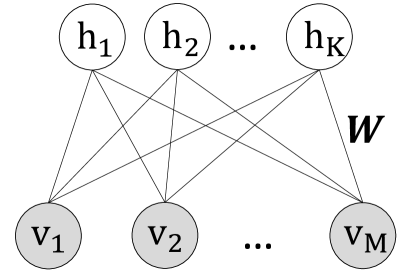
Figure 1: A restricted Boltzmann machine architecture of $M$ visible units and $K$ hidden units.

Model representation

Let use consider an RBM with $M$ visible variables $\boldsymbol{v}=\left\{v_{1},v_{2},\ldots,v_{M}\right\}\in\left\{0,1\right\}^{M}$ and $K$ latent variables $\boldsymbol{h}=\{h_{1},h_{2},...,h_{K}\}\in\{0,1\}^{K}$. The model is parameterized by two bias vectors $\boldsymbol{a}=\{a_{1},a_{2},...,a_{M}\}\in\mathbb{R}^{M}$ in the visible layer and $\boldsymbol{b}=\{b_{1},b_{2},...,b_{M}\}\in\mathbb{R}^{K}$ in the hidden layer and a weight matrix $\boldsymbol{W}\in\mathbb{R}^{M\times K}$ whose element $w_{ij}$ is the weight of the edge from the visible unit $v_{i}$ and the hidden unit $h_{j}$. The set $\boldsymbol{\psi}=\{\boldsymbol{a},\boldsymbol{b},\mathbf{W\}}$ describes the network parameters and specifies RBM’s power.

Similar to Boltzmann machines, an RBM is an energy-based model and its energy value, defined at a particular value of a pair $\boldsymbol{v}$ and $\boldsymbol{h}$, is given by:

$$E(\boldsymbol{v},\boldsymbol{h};\boldsymbol{\psi}) =-(\mathbf{a^{\top}}\boldsymbol{v}+\boldsymbol{b}^{\top}\boldsymbol{h}+\boldsymbol{v}^{\top}\boldsymbol{W})$$ (3)

Following Boltzmann distribution, as known as Gibbs distribution, the joint probability is defined via the energy function as:

$$p(\boldsymbol{v},\boldsymbol{h};\boldsymbol{\psi}) =\frac{1}{\mathcal{Z}(\boldsymbol{\psi})}e^{-E(\boldsymbol{v},\boldsymbol{h};\boldsymbol{\psi})}$$ (4)

where, $\mathcal{Z}(\boldsymbol{\psi})$ is the partition function which is the sum of $e^{-E(\boldsymbol{v},\boldsymbol{h};\boldsymbol{\psi})}$ over all possible pairwise configurations of visible and hidden units in the network, and therefore it guarantees that $p(\boldsymbol{v},\boldsymbol{h};\boldsymbol{\psi})$ is a proper distribution.

$$\mathcal{Z}\left(\boldsymbol{\psi}\right)=\sum_{\boldsymbol{v},\boldsymbol{h}}e^{-E(\boldsymbol{v},\boldsymbol{h};\boldsymbol{\psi})}$$ (5)

By marginalizing Eq. 4 out latent variables $\boldsymbol{h}$, we obtain the data likelihood which assigns a probability to each observed data $\boldsymbol{v}$:

$$p(\boldsymbol{v};\psi) = \frac{1}{\mathcal{Z}(\psi)}\sum_{\boldsymbol{h}}e^{-E(\boldsymbol{v},\boldsymbol{h};\psi)}$$ (6)

Thanks to the special bipartite structure, RBMs offer a convenient way to compute the conditional probabilities $p(\boldsymbol{v}|\boldsymbol{h};\boldsymbol{\psi})$ and $p(\boldsymbol{h}|\boldsymbol{v};\boldsymbol{\psi})$. Indeed, since units in a layer are conditionally independent of units in the other layer, the conditional probabilities can be nicely factorized as

$$p(\boldsymbol{v}|\boldsymbol{h};\boldsymbol{\psi}) =\prod_{i=1}^{M}p(v_{i}|\boldsymbol{h};\boldsymbol{\psi})\qquad p(v_{i}=1|\boldsymbol{h},\boldsymbol{\psi})=\sigma(a_{i}+\mathbf{w}_{i\cdotp}\boldsymbol{h})$$ (7)

$$p(\boldsymbol{h}|\boldsymbol{v};\boldsymbol{\psi}) =\prod_{j=1}^{K}p(h_{j}|\boldsymbol{v};\boldsymbol{\psi})\qquad p(h_{j}=1|\boldsymbol{v},\boldsymbol{\psi})=\sigma(b_{j}+\boldsymbol{v}\mathbf{{}^{\top}w}_{\cdotp j})$$ (8)

where $\sigma\left(x\right)=1/\left(1+e^{-x}\right)$ is a logistic function. In other words, the factorial property allows us to represent the conditional distribution over a layer as the product of the distributions over individual random variables in the layer.

Parameter estimation

As a member of energy-based models, the RBM training aims to search for a parameter set $\hat{\boldsymbol{\psi}}$ that minimizes the network energy. According to the inverse proportion between the data likelihood and the energy function in Eq. 6, the optimization is restated as maximizing the log-likelihood of observed data $\boldsymbol{v}$:

$$\log\mathcal{L}\left(\boldsymbol{v}\right)=\log p(\boldsymbol{v};\boldsymbol{\psi})=\sum_{\boldsymbol{h}}p(\boldsymbol{v},\boldsymbol{h};\boldsymbol{\psi})$$ (9)

Unfortunately, since the maximal points of $\log\mathcal{L}\left(\boldsymbol{v}\right)$ cannot be expressed in the closed-form, a gradient ascent procedure is usually used to iteratively update the parameters in the gradient direction

$$\boldsymbol{\psi} =\boldsymbol{\psi}+\eta\nabla\log\mathcal{L}\left(\boldsymbol{v}\right)$$ (10)

wherein, $\eta$ is a pre-defined learning rate and the gradient vector $\nabla\log\mathcal{L}\left(\boldsymbol{v}\right)$ is computed as follows:

$$\frac{\partial\log\mathcal{L}(\boldsymbol{v};\boldsymbol{\psi})}{\partial\boldsymbol{\psi}} =\mathbb{E}_{p\left(\boldsymbol{h}|\boldsymbol{v};\boldsymbol{\psi}\right)}[-\frac{\partial E(\boldsymbol{v},\boldsymbol{h};\boldsymbol{\psi})}{\partial\boldsymbol{\psi}}]-\mathbb{E}_{p\left(\boldsymbol{v},\boldsymbol{h};\boldsymbol{\psi}\right)}[-\frac{\partial E(\boldsymbol{v},\boldsymbol{h};\boldsymbol{\psi})}{\partial\boldsymbol{\psi}}]$$ (11)

The first term on the right-hand side, denoted $\mathbb{E}_{p\left(\boldsymbol{h}|\boldsymbol{v};\boldsymbol{\psi}\right)}$, is called the data expectation (also known as the positive phase) that is the expected value over the posterior distribution of given data $\boldsymbol{v}$ whilst the second expectation, $\mathbb{E}_{p\left(\boldsymbol{v},\boldsymbol{h};\boldsymbol{\psi}\right)}$, is known as the model expectation (or the negative phase) that is the statistics over the model distribution defined in Eq. 4. For general Boltzmann machines, both terms are intractable, and hence it is not easy to learn a Boltzmann machine. Interestingly, by factorizing conditional probability $p\left(\boldsymbol{h}|\boldsymbol{v};\boldsymbol{\psi}\right),$ RBMs can compute the data expectation analytically. However, the second expectation evaluation is still a challenging problem. To overcome this issue, Markov chain Monte Carlo is widely-used to approximate such expectation. More especially, the capability of conditional probability factorization in RBMs enables us to do sampling efficiently using Gibbs sampling (Geman and Geman, 1984). Intuitively, we alternatively draw hidden and visible samples from the conditional probability distributions given the other variables (Eqs. 7 and 8), $\tilde{\boldsymbol{h}}\sim p(\boldsymbol{h}|\boldsymbol{v};\boldsymbol{\psi})$ and $\tilde{\boldsymbol{v}}\sim p(\boldsymbol{v}|\boldsymbol{h};\boldsymbol{\psi})$, in one Gibbs sampling step. To gain the unbiased estimate of the gradient, it is necessary for the Markov chain to converge to the equilibrium distribution. By this way, the training is viewed as adjusting the parameters to minimize the Kullback-Lieber divergence between the data distribution and the equilibrium distribution. To speed up the approximation process, Hinton proposed to use contrastive divergence with $m$ Gibbs sampling steps (denoted $\text{CD}_{m}$) to evaluate the model expectation. He argued that when the Markov chain converges, the distributions between two consecutive sampling steps are almost the same. As a result, $\text{CD}_{m}$ minimizes the difference between the data distribution and the $m$-sampling step distribution rather than equilibrium distribution. Although contrastive divergence is fast and has low variance, it is still far from the equilibrium distribution if the mixing rate is low. An alternative is persistent contrastive divergence (PCD)(Tieleman, 2008). Unlike CD whose MCMC chain is restarted for each data sample, PCD’s chain is only reset after a regular interval or not reset at all. Furthermore, PCD maintains several chains, usually equal to the batch size, at the same time to achieve a better approximation. Fig. 2 demonstrates the alternative steps of Gibbs sampler, where $\text{CD}_{m}$ is considered as its truncated version with the first $m+1$ steps. $\text{CD}_{1}$ is common in practice since it shows a large improvement in training time with only a small bias (Carreira-Perpinan and Hinton, 2005).

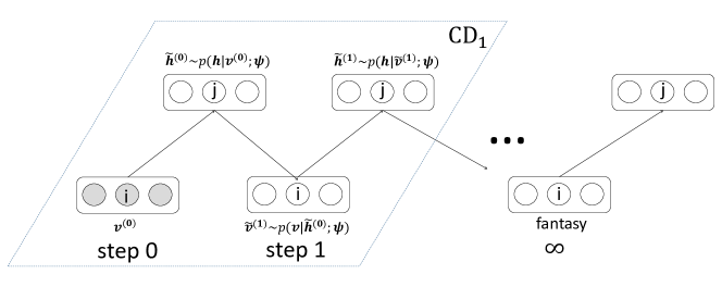
Figure 2: An illustration of Gibbs sampling and 1-step contrastive divergence.

Data reconstruction

Once the optimal parameters $\hat{\boldsymbol{\psi}}$ are learned, the model can be used to obtain the reconstructed data $\tilde{\boldsymbol{v}}$ whenever supplying an input data $\boldsymbol{v}$. Firstly, by propagating the input vector to the hidden layer, we acquire its new representation $\tilde{\boldsymbol{h}}=\left(\tilde{h}_{1},\tilde{h}_{2},...,\tilde{h}_{K}\right)^{\top}$ in the hidden space as follows:

$$\tilde{h}_{k}\sim p\left(h_{k}=1\mid\boldsymbol{v}\right)=\sigma\left(b_{k}+\sum_{m}w_{mk}v_{m}\right)$$ (12)

The hidden sample vector $\tilde{\boldsymbol{h}}$ is then mapped back to the input space for the reconstructed data $\tilde{\boldsymbol{v}}=\left[\tilde{v}_{1},\tilde{v}_{2},...,\tilde{v}_{M}\right]^{\top}$ where

$$\tilde{v}_{m}\sim p\left(v_{m}=1\mid\tilde{\boldsymbol{h}};\psi\right)=\sigma\left(a_{m}+\sum_{k}w_{mk}\tilde{h}_{k}\right)$$ (13)

The forward and backward propagations in Eqs. 12 and 13 are done effectively because of the nice factorisation nature of RBMs. More practically, the reconstructed data can be used to recover the missing or corrupted elements in $\boldsymbol{v}$ (caused by sensory errors or transmission noises) or do classification (Larochelle and Bengio, 2008) while the high difference between $\boldsymbol{v}$ and $\dot{\boldsymbol{v}}$ indicates an occurrence of anomaly signals or data.

3.2 Framework

We propose a unified framework for anomaly detection in video based on the restricted Boltzmann machine (RBM) (Freund and Haussler, 1994; Hinton, 2002). Our proposed system employs RBMs as core modules to model the complex distribution of data, capture the data regularity and variations (Nguyen et al., 2015), as a result effectively reconstruct the normal events that occur frequently in the data. The idea is to use the errors of reconstructed data to recognize the abnormal objects or behaviours that deviate significantly from the common.

Our framework is trained in a completely unsupervised manner that does not involve any explicit labels or implicit knowledge of what to be defined as abnormal. In addition, it can work directly on raw pixels without the need for expensive feature engineering procedure. Another advantage of our method is the capability of detecting the exact boundary of local abnormality in video frames. To handle the video data coming in a stream, we further extend our method to incrementally update parameters without retraining the models from scratch. Our solution can be easily deployed in arbitrary surveillance streaming setting without the expensive calibration requirement.

We now describe our proposed framework that is based on the RBM to detect anomaly events for each frame in video data. In general, our system is a two-phase pipeline: training phase and detecting phase. Particularly in the training phase, our model: (i) takes a series of video frames in the training data as a collection of images, (ii) divides each image into patches, (iii) gathers similar patches into clusters, and (iv) learns separate RBM for each cluster using the image patches. The detecting phase consists of three steps: (i) collecting image patches in the testing video for each cluster, and then using the learned RBM to reconstruct the data for the corresponding cluster of patches, (ii) proposing the regions that are potential to be abnormal by applying a predefined threshold to reconstruction errors, and then finding connected components of these candidates and filtering out those too small, and (iii) updating the model incrementally for the data stream. The overview of our framework is illustrated in Fig. 3. In what follows, we describe training and detecting phases in more details.

Training phase.

Assume that the training data consists of $N$ video frames with the size of $H\times W$ pixels, let denote $\mathcal{D}=\{\boldsymbol{x}_{t}\in\mathbb{R}^{H\times W}\}_{t=1}^{N}$. In real-life video surveillance data, $H\times W$ is usually very large (e.g., hundreds of thousand pixels), hence it is often infeasible for a single RBM to handle such high-dimensional image. This is because the high-dimensional input requires a more complex model with an extremely large number of parameters (i.e., millions). This makes the parameter learning more difficult and less robust since it is hard to control the bounding of hidden activation values. Thus the hidden posteriors are easily collapsed into either zeros or ones, and no more learning occurs.

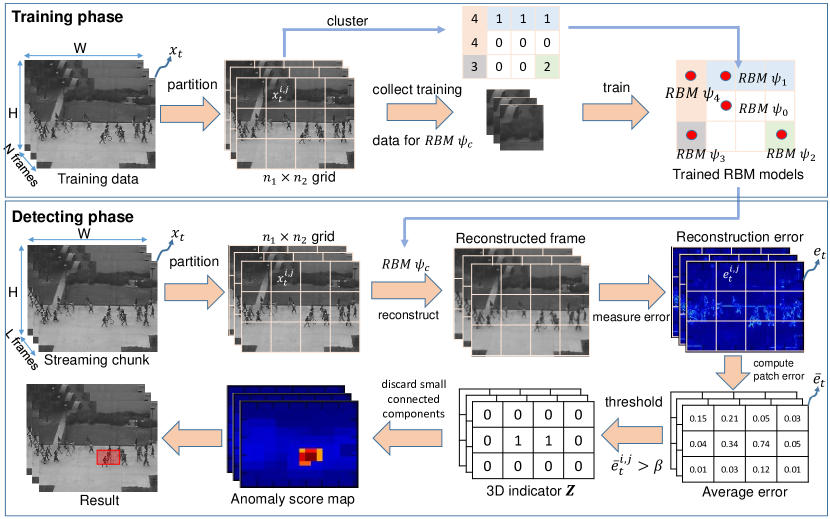
Figure 3: The overview of our proposed framework.

To tackle this issue, one can reduce the data dimension using dimensionality reduction techniques or by subsampling the image to smaller size. This solution, however, is computational demanding and may lose much information of the original data. In this work we choose to apply RBMs directly to raw imaginary pixels whilst try to preserve information. To that end, we train our model on $h\times w$ patches where we divide each image $\boldsymbol{x}_{t}$ into a grid of $N_{h}\times N_{w}$ patches: $\boldsymbol{x}_{t}=\{\boldsymbol{x}_{t}^{i,j}\mid 1\leq i\leq N_{h},1\leq j\leq N_{w}\}$. This approach greatly reduces the data dimensionality and hence requires smaller models. One way is to learn independent RBMs on patches at each location ($i,j$). However, this would result in an excessive number of models, for example, $400$ RBMs to work on the $240\times 360$ image resolution and $12\times 18$ patch size, hence leading to very high computational complexity and memory demand.

Our solution is to reduce the number of models by grouping all similar patches from different locations for learning a single model. We observe that it is redundant to train a separate model for each location of patches since most adjacent patches such as pathways, walls and nature strips in surveillance scenes have similar appearance and texture. Thus we first train an RBM with a small number of hidden units ($K=4$) on all patches $\{\boldsymbol{x}_{t}^{i,j}\}$ of all video frames. We then compute the hidden posterior $\tilde{\boldsymbol{h}}$ for each image patch $\boldsymbol{x}_{t}^{i,j}$ and binarize it to obtain the binary vector: $\tilde{\boldsymbol{h}}=\left[\mathbb{I}\left(\tilde{h}_{1}>0.5\right),...,\mathbb{I}\left(\tilde{h}_{K}>0.5\right)\right]$ where $\mathbb{I}\left(\bullet\right)$ is the indicator function. Next this binary vector is converted to an integer value in decimal system, e.g., 0101 converted to 5, which we use as the pseudo-label $\lambda_{t}^{i,j}$ of the cluster of the image patch $\boldsymbol{x}_{t}^{i,j}$. The cluster label $c^{i,j}$ for all patches at location ($i,j$) is chosen by voting the pseudo-labels over all $N$ frames: $\lambda_{1}^{i,j},\lambda_{2}^{i,j},...,\lambda_{N}^{i,j}$. Let $C$ denote the number of unique cluster labels in the set {$c^{i,j}\mid 1\leq i\leq N_{h},1\leq j\leq N_{w}$}, we finally train $C$ independent RBMs with a larger number of hidden units ($K=100$), each with parameter set $\psi_{c}$ for all patches with the same cluster label $c$.

Detecting phase.

Once all RBMs have been learned using the training data, they are used to reveal the irregular events in the testing data. The pseudocode of this phase is given in Alg. 1. Overall, there are three main steps: reconstructing the data, detecting local abnormal objects and updating models incrementally. In particular, the stream of video data is first split into chunks of $L$ non-overlapping frames, each denoted by $\left\{\boldsymbol{x}_{t}\right\}_{t=1}^{L}$. Each patch $\boldsymbol{x}_{t}^{i,j}$ is then reconstructed to obtain the reconstruction $\tilde{\boldsymbol{x}}_{t}^{i,j}$ using the learned RBM with parameters $\psi_{c^{i,j}}$, and all together form the reconstructed data $\tilde{\boldsymbol{x}}_{t}$ of the frame $\boldsymbol{x}_{t}$. The reconstruction error $\boldsymbol{e}_{t}=[\boldsymbol{e}_{t}^{i,j}]\in\mathbb{R}^{H\times W}$ is then computed as: $\boldsymbol{e}_{t}^{i,j}=|\boldsymbol{x}_{t}^{i,j}-\tilde{\boldsymbol{x}}_{t}^{i,j}|$.

To detect abnormal pixels, one can compare the reconstruction error $\boldsymbol{e}_{t}$ with a given threshold. This approach, however, may produce many false alarms when normal pixels are reconstructed with high errors, and may fail to cover the entire abnormal objects in such a case that they are fragmented into isolated high error parts. Our solution is to work on the average error $\bar{e}_{t}^{i,j}=||\boldsymbol{e}_{t}^{i,j}||_{2}/\left(h\times w\right)$ over patches rather than individual pixels. These errors are then compared with a predefined threshold $\beta$. All pixels in the patch $\boldsymbol{x}_{t}^{i,j}$ are considered abnormal if $\bar{e}_{t}^{i,j}\geq\beta$.

Applying the above procedure and then concatenating $L$ frames, we obtain a binary 3D rectangle $\boldsymbol{Z}\in\left\{0,1\right\}^{L\times H\times W}$ wherein $z_{i,j,k}=1$ indicates the abnormal voxel whilst $z_{i,j,k}=0$ the normal one. Throughout the experiments, we observe that most of abnormal voxels in $\boldsymbol{Z}$ are detected correctly, but there still exist several small groups of voxels are incorrect. We further filter out these false positive voxels by connecting all their related neighbors. More specifically, we first build a sparse graph whose nodes are abnormal voxels $z_{i,j,k}=1$ and edges are the connections of these voxels with their abnormal neighbours $z_{i+u,j+v,k+t}=1$ where $u,v,t\in\left\{-1,0,1\right\}$ and $\left|u\right|+\left|v\right|+\left|t\right|>0$. We then find all connected components in this graph, and discard small components spanning less than $\gamma$ contiguous frames. The average error $\bar{e}_{t}^{i,j}$ after this component filtering step can be used as final anomaly score.

1: Video chunk $\left\{\boldsymbol{x}_{t}\right\}_{t=1}^{L}$, models $\left\{\psi_{c}\right\}_{c=1}^{C}$, thresholds $\beta$ and $\gamma$

2:Detection $\boldsymbol{Z}$, score $\left\{\bar{e}_{t}^{i,j}\right\}$

3:for $t\leftarrow 1,\ldots,L$ do

4:     for $\boldsymbol{x}_{t}^{i,j}\in\boldsymbol{x}_{t}$ do

5:         $\tilde{\boldsymbol{x}}_{t}^{i,j}\leftarrow$reconstruct($\boldsymbol{x}_{t}^{i,j}$,$\psi_{c^{i,j}}$)

6:         $\boldsymbol{e}_{t}^{i,j}\leftarrow|\boldsymbol{x}_{t}^{i,j}-\tilde{\boldsymbol{x}}_{t}^{i,j}|$

7:         $\bar{e}_{t}^{i,j}\leftarrow\frac{1}{h\times w}\left\|\boldsymbol{e}_{t}^{i,j}\right\|_{2}$

8:         if $\bar{e}_{t}^{i,j}\geq\beta$ then

9:              for $p\in\boldsymbol{x}_{t}^{i,j}$ do

10:                  $\boldsymbol{Z}(p)\leftarrow 1$

11:              end for

12:         else

13:              for $p\in\boldsymbol{x}_{t}^{i,j}$ do

14:                  $\boldsymbol{Z}(p)\leftarrow 0$

15:              end for

16:         end if

17:     end for

18:     for $c\leftarrow 1,\ldots,C$ do

19:         $\boldsymbol{X}_{t}^{c}\leftarrow\left\{\boldsymbol{x}_{t}^{i,j}\mid c^{i,j}=c\right\}$

20:         $\psi_{c}\leftarrow\text{{updateRBM}}(\boldsymbol{X}_{t}^{c},\psi_{c})$

21:     end for

22:end for

23:$\boldsymbol{Z}\leftarrow$remove_small_components($\boldsymbol{Z},$$\gamma$)

Algorithm 1 RBM anomaly detection

In the scenario of streaming videos, the scene frequently changes over time and it could be significantly different from those are used to train RBMs. To tackle this issue, we further extend our proposed framework to enable the RBMs to adapt themselves to the new video frames. For every incoming frame $t$, we extract the image patches and update the parameters $\psi_{1:C}$ of $C$ RBMs in our framework following the procedure in the training phase. Recall that the RBM parameters are updated iteratively using gradient ascent, thus here we use several epochs to ensure the information of new data are sufficiently captured by the models.

One problem is the anomalous objects can be presented in different sizes in the video. To deal with this issue, we apply our framework to the video data at different scales whilst keeping the same patch size $h\times w$. This would help the patch partially or entirely cover objects at certain scales. To that end, we rescale the original video into different resolutions, then employ the same procedure above to compute the average reconstruction error map $\bar{e}_{t}$ and 3D rectangular indicators $\boldsymbol{Z}$. The average error maps are then aggregated into one matrix using max operation. Likewise, indicator tensors are merged into one before finding the connected components. We also use overlapping patches to localize anomalous objects more accurately. Pixels in the overlapping regions are averaged when combining patches into the whole map.

4 Results

In this section, we empirically evaluate the performance of our anomaly detection framework both qualitatively and quantitatively. Our aim is to investigate the capabilities of capturing data regularity, reconstructing the data and detecting local abnormalities of our system. For quantitative analysis, we compare our proposed method with several up-to-date baselines.

We use 3 public datasets: UCSD Ped 1, Ped 2 (Li et al., 2014) and Avenue (Lu et al., 2013). Under the unsupervised setting, we disregard labels in the training videos and train all methods on these videos. The learned models are then evaluated on the testing videos by computing 2 measures: area under ROC curve (AUC) and equal error rate (EER) at frame-level (no anomaly object localization evaluation) and pixel-level (40% of ground-truth anomaly pixels are covered by detection), following the evaluation protocol used in (Li et al., 2014) and at dual-pixel level (pixel-level constraint above and at least $\alpha$ percent of detection is true anomaly pixels) in (Sabokrou et al., 2015). Note that pixel-level is a special case of dual-pixel where $\alpha=0$. Since the videos are provided at different resolution, we first resize all into the same size of $240\times 360$.

For our framework, we duplicate and rescale video frames to multi-scale copies with the ratios of $1.0$, $0.5$ and $0.25$, and then use $12\times 18$ image patches with $50\%$ overlapping between two adjacent patches. Each RBM now consists of $216$ visible units and $4$ hidden units for clustering step whilst $100$ hidden units for training and detecting phases. All RBMs are trained using $\text{CD}_{1}$ with learning rate $\eta=0.1$. To simulate the streaming setting, we split testing videos in non-overlapping chunks of $L=20$ contiguous frames and use $20$ epochs to incrementally update parameters of RBMs. The thresholds $\beta$ and $\gamma$ to determine anomaly are set to $0.003$ and $10$ respectively. Those hyperparameters have been tuned to reduce false alarms and to achieve the best balanced AUC and EER scores.

4.0.1 Region Clustering

In the first experiment, we examine the clustering performance of RBM. Fig. 4 shows the cluster maps discovered by RBM on three datasets. Using $4$ hidden units, the RBM can produce a maximum of $16$ clusters, but in fact, the model returns less and varied number of clusters for different datasets at different scales. For example, ($6$, $7$, $10$) similar regions at scales ($1.0$, $0.5$, $0.25$) are found for Ped 1 dataset, whilst these numbers for Ped 2 and Avenue dataset are ($9$, $9$, $8$) and ($6$, $9$, $9$) respectively. This suggests the capability of automatically selecting the appropriate number of clusters of RBM.

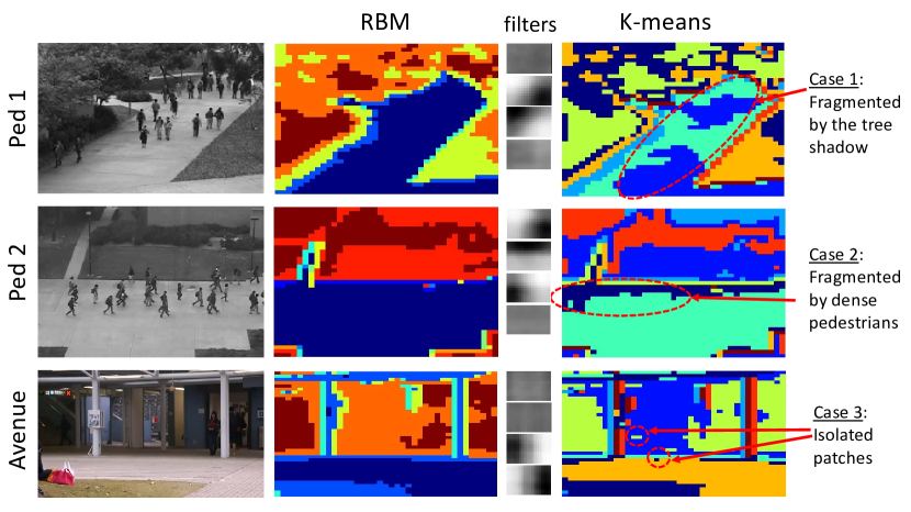
Figure 4: Clustering results on some surveillance scenes at the first scale: (first column) example frames; (second) cluster maps produced by RBM; (third) filters learned by RBM; and (fourth) cluster maps produced by $k$-means.

For comparison, we run $k$-means algorithm with $k=8$ clusters, the average number of clusters of RBM. It can be seen from Fig. 4 that the $k$-means fails to connect large regions which are fragmented by the surrounding and dynamic objects, for example, the shadow of tree on the footpath (Case 1), pedestrians walking at the upper side of the footpath (Case 2). It also assigns several wrong labels to small patches inside a larger area as shown in Case 3. By contrast, the RBM is more robust to the influence of environmental factors and dynamic foreground objects, and thus produces more accurate clustering results. Taking a closer look at the filters learned by RBM at the third column in the figure, we can agree that the RBM learns the basic features such as homogeneous regions, vertical, horizontal, diagonal edges and corners, which then can be combined to construct the entire scene.

4.0.2 Data Reconstruction

We next demonstrate the capability of our framework on the data reconstruction. Fig. 5 shows an example of reconstructing the video frame in Avenue dataset. Here the abnormal object is a girl walking toward the camera. It can be seen that our model can correctly locate this outlier behaviour based on the reconstruction errors shown in figures (c) and (d). This is because the RBM can capture the data regularity, thus produces low reconstruction errors for regular objects and high errors for irregular or anomalous ones as shown in figures (b) and (c).

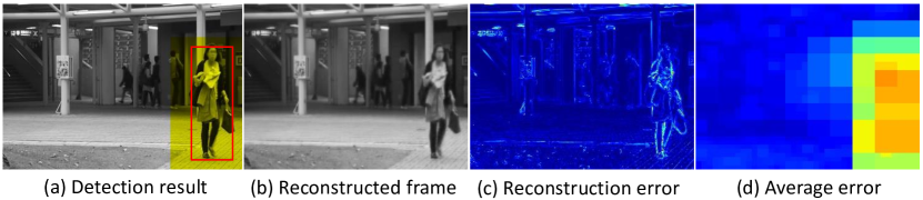
Figure 5: Data reconstruction of our method on Avenue dataset: (a) the original frame with detected outlier female (yellow region) and ground-truth (red rectangle), (b) reconstructed frame, (c) reconstruction error image, (d) average reconstruction errors of patches.

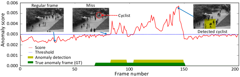
Figure 6: Average reconstruction error per frame in test video #1 of UCSD Ped 1 dataset. The shaded green region illustrates anomalous frames in the ground truth, while the yellow anomalous frames detected by our method. The blue line shows the threshold.

To examine the change of reconstruction errors in a stream of video frames, we visualize the maximum average reconstruction error in a frame as a function of frame index as shown in Fig. 6. The test video #1 in UCSD Ped 1 dataset contains some normal frames of walking on a footpath, followed by the appearance of a cyclist moving towards the camera. Our system could not detect the emergence of the cyclist since the object is too small and cluttered by many surrounding pedestrians. However, after several frames, the cyclist is properly spotted by our system with the reconstruction errors far higher than the threshold.

4.0.3 Anomaly Detection Performance

In the last investigation, we compare our offline RBM framework and its streaming version (called S-RBM) with the unsupervised methods for anomaly detection in the literature. We use 4 baselines for comparison: principal component analysis (PCA), one-class support vector machine (OC-SVM) (Amer et al., 2013), Gaussian mixture models (GMM), and convolutional autoencoder (ConvAE) (Hasan et al., 2016). We use the variant of PCA with optical flow features from (Saha et al., 2009), and adopt the results of ConvAE from the original work (Hasan et al., 2016). The results of ConvAE are already compared with recent state-of-the-art baselines including supervised methods.

We follow similar procedures to what of our proposed framework for OC-SVM and GMM, but apply these baselines on image patches clustered by $k$-means. The kernel width and lower bound of the fraction of support vectors of OC-SVM are set to $0.1$ and $10^{-4}$ respectively. In GMM model, the number of Gaussian components is set to 20 and the anomaly threshold is -50. These hyperparameters are also tuned to obtain the best cross-validation results. It is noteworthy that it is not straightforward to implement the incremental versions of the baselines, thus we do not include them here.

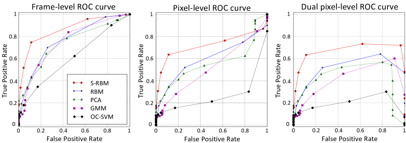
Figure 7: Comparison ROC curves on UCSD Ped 2. Three figures share the same legend. Higher curves indicate better performance. It is notable that, unlike frame and pixel-level evaluations, dual-pixel level curves may end at any points lower than (1,1).

The ROC curves are shown in Fig. 7 whilst AUC and EER scores are reported in Table 1. Both RBM and S-RBM outperform the PCA, OC-SVM, GMM with higher AUC and lower EER scores. Specially, our methods can produce higher AUC scores at dual pixel-level which shows better quality in localizing anomaly regions. Additionally, S-RBM achieves fairly comparable results with the ConvAE. It is noteworthy that the ConvAE is a 12-layer deep architecture consisting of sophisticated connections between its convolutional and pooling layers. On the other hand, our RBM anomaly detector has only two layers, but obtains a respectable performance. We believe that our proposed framework is a promising system to detect abnormalities in video surveillance applications.

	Ped1					Ped2					Avenue
	Frame		Pixel		Dual	Frame		Pixel		Dual	Frame		Pixel		Dual
	AUC	EER	AUC	EER	AUC	AUC	EER	AUC	EER	AUC	AUC	EER	AUC	EER	AUC
PCA	60.28	43.18	25.39	39.56	8.76	73.98	29.20	55.83	24.88	44.24	74.64	30.04	52.90	37.73	43.74
OC-SVM	59.06	42.97	21.78	37.47	11.72	61.01	44.43	26.27	26.47	19.23	71.66	33.87	33.16	47.55	33.15
GMM	60.33	38.88	36.64	35.07	13.60	75.20	30.95	51.93	18.46	40.33	67.27	35.84	43.06	43.13	41.64
ConvAE	81.00	27.90	_	_	_	90.00	21.70	_	_	_	70.20	25.10	_	_	_
RBM	64.83	37.94	41.87	36.54	16.06	76.70	28.56	59.95	19.75	46.13	74.88	32.49	43.72	43.83	41.57
S-RBM	70.25	35.40	48.87	33.31	22.07	86.43	16.47	72.05	15.32	66.14	78.76	27.21	56.08	34.40	53.40

Table 1: Anomaly detection results (AUC and EER) at frame-level, pixel-level and dual pixel-level ($\alpha=5\%)$ on 3 datasets. Higher AUC and lower EER indicate better performance. Meanwhile, high dual-pixel values point out more accurate localization. We do not report EER for dual-pixel level because this number do not always exist. Best scores are in bold. Note that the frame-level results of ConvAE are taken from (Hasan et al., 2016), but the pixel-level and dual-pixel level results are not available.

5 Discussion and Future Work

5.1 Drawbacks and Future Plans

Although our RBM-based anomaly detection system has proven an excellent performance in the experiments, RBMs are just shadow generative networks with two layers. The direct extension to deep generative networks such DBNs (Hinton et al., 2006) or DBMs (Salakhutdinov and Hinton, 2009) offers more powerful capacity of encoding the normality distribution and produces superior detection performance. In the future, we intend to integrate the deep architecture into our anomaly framework and discover effective mechanism to train and do inference in such multi-layer generative nets. For further extension, we aim to develop a deep abnormality detection system that is a deep generative network specialising in the problem of anomaly detection, instead of adapting the popular deep networks in literature that are designed for general purpose.

5.2 Significance and Benefits

Our research introduces an effective framework to detect anomaly events in streaming surveillance videos. Broadly speaking, the significance of our work lies on developing a powerful and generalized tool with capacity of unsupervised learning, automatic representation and less need for human-intervention that enables to isolate unexpected signals and unusual patterns in data collection. This research also develops a comprehensive understanding of the usage of generative networks for anomaly detection. By analysing their strengths and drawbacks, we can design more efficient and effective networks that specialize to localize abnormal data points. However, the multi-layer architecture in deep networks inspires us with the idea of hierarchical anomaly detection systems where anomaly data (e.g. unusual pixels or regions in video frames) are detected in the bottom layers and abstract anomaly information (e.g. anomaly scenes in videos) is represented in the top layers. Finally, many practical applications such as video analysis, fraud detection, structural defect detection, medical anomaly detection will benefit from our proposed system.

6 Conclusion

Throughout this report, we have described the current research trend in the problem of anomaly detection, and more specifically, video anomaly detection. We also have summarized the recent studies of generative networks that are grounded in deep learning and neural network principles. The literature review pointed out three key limitations of existing anomaly detectors that are insufficient labeled data, the ambiguous definition of abnormality and the costly step of feature representation. To overcome these limitations, we have introduced our idea of utilising the power of generative networks to model the regular data distribution using restricted Boltzmann machines, and then detect anomaly events via reconstruction errors. We conducted the experiments on three benchmark datasets of UCSD Ped1, Ped2 and Avenue for video anomaly detection and compared our network with several baselines. The experimental results show that our shallow network can obtain the comparable performance with the state-of-the-art anomaly detectors. In future work, we aim to build a deep anomaly detection system that is specially designed for anomaly detection. Many application domains, including video analysis and scene understanding, can benefit from the results of our research.

References

- Ackley et al. [1985] David H. Ackley, Geoffrey E. Hinton, and Terrence J. Sejnowski. A learning algorithm for boltzmann machines. Cognitive Science, 9(1):147 – 169, 1985. ISSN 0364-0213. doi: http://dx.doi.org/10.1016/S0364-0213(85)80012-4. URL http://www.sciencedirect.com/science/article/pii/S0364021385800124.
- Ajtai [1983] M. Ajtai. -formulae on finite structures. Annals of Pure and Applied Logic, 24(1):1 – 48, 1983. ISSN 0168-0072. doi: http://dx.doi.org/10.1016/0168-0072(83)90038-6. URL http://www.sciencedirect.com/science/article/pii/0168007283900386.
- Allender [1996] Eric Allender. Circuit complexity before the dawn of the new millennium. In Proceedings of the 16th Conference on Foundations of Software Technology and Theoretical Computer Science (FSTTCS), pages 1–18, Hyderabad, India, December 18-20 1996. doi: 10.1007/3-540-62034-6˙33. URL http://dx.doi.org/10.1007/3-540-62034-6_33.
- Amer et al. [2013] Mennatallah Amer, Markus Goldstein, and Slim Abdennadher. Enhancing one-class support vector machines for unsupervised anomaly detection. In Proceedings of the ACM Special Interest Group on Knowledge Discovery and Data Mining (SIGKDD) Workshop on Outlier Detection and Description, ODD ’13, pages 8–15, New York, USA, 2013. ACM. ISBN 978-1-4503-2335-2. doi: 10.1145/2500853.2500857. URL http://doi.acm.org/10.1145/2500853.2500857.
- Basharat et al. [2008] Arslan Basharat, Alexei Gritai, and Mubarak Shah. Learning object motion patterns for anomaly detection and improved object detection. In Proceedings of Conference on Computer Vision and Pattern Recognition (CVPR), pages 24–26, Anchorage, Alaska, USA, June 2008. doi: 10.1109/CVPR.2008.4587510. URL http://dx.doi.org/10.1109/CVPR.2008.4587510.
- Benezeth et al. [2009] Y. Benezeth, P.-M. Jodoin, V. Saligrama, and C. Rosenberger. Abnormal events detection based on spatio-temporal co-occurences. In Proceedings of Conference on Computer Vision and Pattern Recognition (CVPR), June 2009. doi: 10.1109/cvpr.2009.5206686. URL http://dx.doi.org/10.1109/CVPR.2009.5206686.
- Bengio and LeCun [2007] Yoshua Bengio and Yann LeCun. Scaling learning algorithms towards AI. In Large Scale Kernel Machines. MIT Press, 2007. URL http://www.iro.umontreal.ca/~lisa/pointeurs/bengio+lecun_chapter2007.pdf.
- Bengio et al. [2007] Yoshua Bengio, Pascal Lamblin, Dan Popovici, and Hugo Larochelle. Greedy layer-wise training of deep networks. In Advances in Neural Information Processing Systems (NIPS), pages 153–160. MIT Press, 2007. URL http://papers.nips.cc/paper/3048-greedy-layer-wise-training-of-deep-networks.pdf.
- Besag [1975] Julian Besag. Statistical analysis of non-lattice data. Journal of the Royal Statistical Society, 24(3):179–195, 1975. ISSN 00390526. URL http://www.jstor.org/stable/2987782.
- Bornschein and Bengio [2015] Jörg Bornschein and Yoshua Bengio. Reweighted wake-sleep. The 5th International Conference on Learning Representation (ICLR), abs/1406.2751, 2015. URL http://arxiv.org/abs/1406.2751.
- Bornschein et al. [2015] Jörg Bornschein, Samira Shabanian, Asja Fischer, and Yoshua Bengio. Bidirectional helmhltz machines. The 32nd International Conference on Machine Learning (ICML), abs/1506.03877, 2015. URL http://arxiv.org/abs/1506.03877.
- Boulanger-Lewandowski et al. [2012] Nicolas Boulanger-Lewandowski, Yoshua Bengio, and Pascal Vincent. Modeling temporal dependencies in high-dimensional sequences: Application to polyphonic music generation and transcription. In Proceedings of the 29th International Conference on Machine Learning (ICML), 2012.
- Brunet et al. [2012] Dominique Brunet, Edward R. Vrscay, and Zhou Wang. On the mathematical properties of the structural similarity index. IEEE Transactions on Image Processing, 21(4):1488–1499, apr 2012. doi: 10.1109/tip.2011.2173206. URL http://dx.doi.org/10.1109/TIP.2011.2173206.
- Burda et al. [2016] Yuri Burda, Roger B. Grosse, and Ruslan Salakhutdinov. Importance weighted autoencoders. The 4th International Conference on Learning Representations (ICLR), abs/1509.00519, 2016. URL http://arxiv.org/abs/1509.00519.
- Carreira-Perpinan and Hinton [2005] Miguel A. Carreira-Perpinan and Geoffrey E. Hinton. On contrastive divergence learning. In Intelligence, Artificial and Statistics, Barbados, 2005.
- Chandola et al. [2009] Varun Chandola, Arindam Banerjee, and Vipin Kumar. Anomaly detection: A survey. ACM Computing Surveys (CSUR), 41(3):15:1–15:58, 2009. ISSN 0360-0300. doi: 10.1145/1541880.1541882. URL http://doi.acm.org/10.1145/1541880.1541882.
- Cho et al. [2011] Kyung Hyun Cho, Tapani Raiko, and Alexander Ilin. Enhanced gradient and adaptive learning rate for training restricted boltzmann machines. In Proceedings of the 28th International Conference on Machine Learning ICML, pages 105–112, Bellevue, Washington, USA, June 28 - July 2 2011.
- Chung et al. [2014] Junyoung Chung, Çaglar Gülçehre, KyungHyun Cho, and Yoshua Bengio. Empirical evaluation of gated recurrent neural networks on sequence modeling. The 27th Advances in Neural Information Processing Systems (NIPS), abs/1412.3555, 2014. URL http://arxiv.org/abs/1412.3555.
- Chung et al. [2015] Junyoung Chung, Kyle Kastner, Laurent Dinh, Kratarth Goel, Aaron C. Courville, and Yoshua Bengio. A recurrent latent variable model for sequential data. In the 28th Advances in Neural Information Processing Systems (NIPS), pages 2980–2988, Montreal, Quebec, Canada, December 7-12 2015. URL http://papers.nips.cc/paper/5653-a-recurrent-latent-variable-model-for-sequential-data.
- Clarke [2015] Melissa Clarke. Globally, terrorism is on the rise - but little of it occurs in western countries, 2015. URL http://www.abc.net.au/news/2015-11-17/global-terrorism-index-increase/6947200.
- Courville et al. [2011] Aarron Courville, James Bergstra, and Yoshua Bengio. Unsupervised models of images by spike-and-slab rbms. In Proceedings of the 28th International Conference on Machine Learning (ICML), pages 1145–1152, New York, USA, June 2011. ACM. ISBN 978-1-4503-0619-5.
- Crime Statisticas Agency [2016] Australia Crime Statisticas Agency, Victoria. Recorded offences in the victoria police law enforcement assistance program (leap) database between october 2011 and september 2016, 2016. URL https://www.crimestatistics.vic.gov.au/crime-statistics/latest-crime-data/recorded-offences-1.
- Cui et al. [2011] Xinyi Cui, Qingshan Liu, Mingchen Gao, and Dimitris N. Metaxas. Abnormal detection using interaction energy potentials. In Proceedings of Conference on Computer Vision and Pattern Recognition (CVPR), June 2011. doi: 10.1109/cvpr.2011.5995558. URL http://dx.doi.org/10.1109/CVPR.2011.5995558.
- Dayan and Hinton [1996] Peter Dayan and Geoffrey E. Hinton. Varieties of helmholtz machine. Neural Netw., 9(8):1385–1403, November 1996. ISSN 0893-6080. doi: 10.1016/S0893-6080(96)00009-3. URL http://dx.doi.org/10.1016/S0893-6080(96)00009-3.
- Dayan et al. [1995] Peter Dayan, Geoffrey E. Hinton, Radford M. Neal, and Richard S. Zemel. The Helmholtz machine. Neural Computation, 7:889–904, 1995.
- Denton et al. [2015] Emily L. Denton, Soumith Chintala, Arthur Szlam, and Robert Fergus. Deep generative image models using a laplacian pyramid of adversarial networks. The 28th Advances in Neural Information Processing Systems (NIPS), abs/1506.05751, 2015. URL http://arxiv.org/abs/1506.05751.
- Desjardins and Bengio [2008] Guillaume Desjardins and Yoshua Bengio. Empirical evaluation of convolutional RBMs for vision. Technical Report 1327, Département d’Informatique et de Recherche Opérationnelle, Université de Montréal, 2008.
- Dosovitskiy et al. [2015] Alexey Dosovitskiy, Jost Tobias Springenberg, and Thomas Brox. Learning to generate chairs with convolutional neural networks. In Proceedings of the 28th Conference on Computer Vision and Pattern Recognition (CVPR), pages 1538–1546, Boston, MA, USA, June 7-12 2015. doi: 10.1109/CVPR.2015.7298761. URL http://dx.doi.org/10.1109/CVPR.2015.7298761.
- Duong et al. [2005] Thi V. Duong, Hung H. Bui, Dinh Q. Phung, and Svetha Venkatesh. Activity recognition and abnormality detection with the switching hidden semi-markov model. In Proceedings of the 2005 IEEE Computer Society Conference on Computer Vision and Pattern Recognition (CVPR’05) - Volume 1 - Volume 01, CVPR ’05, pages 838–845, Washington, DC, USA, 2005. IEEE Computer Society. ISBN 0-7695-2372-2. doi: 10.1109/CVPR.2005.61. URL http://dx.doi.org/10.1109/CVPR.2005.61.
- Fahlman et al. [1983] Scott E. Fahlman, Geoffrey E. Hinton, and Terrence J. Sejnowski. Massively parallel architectures for ai: Netl, thistle, and boltzmann machines. In Proceedings of the 3rd AAAI Conference on Artificial Intelligence (AAAI), pages 109–113, 1983. URL http://dl.acm.org/citation.cfm?id=2886844.2886868.
- Fang et al. [2016] Zhijun Fang, Fengchang Fei, Yuming Fang, Changhoon Lee, Naixue Xiong, Lei Shu, and Sheng Chen. Abnormal event detection in crowded scenes based on deep learning. Multimedia Tools and Applications, 75(22):14617–14639, November 2016. ISSN 1380-7501. doi: 10.1007/s11042-016-3316-3. URL http://dx.doi.org/10.1007/s11042-016-3316-3.
- Farabet et al. [2013] Clément Farabet, Camille Couprie, Laurent Najman, and Yann LeCun. Learning hierarchical features for scene labeling. The IEEE Transactions on Pattern Analysis and Machine Intelligence (TPAMI), 35(8):1915–1929, 2013. doi: 10.1109/TPAMI.2012.231. URL http://dx.doi.org/10.1109/TPAMI.2012.231.
- Feng et al. [2017] Yachuang Feng, Yuan Yuan, and Xiaoqiang Lu. Learning deep event models for crowd anomaly detection. Neurocomputing, 219:548 – 556, 2017. ISSN 0925-2312. doi: http://dx.doi.org/10.1016/j.neucom.2016.09.063. URL http://www.sciencedirect.com/science/article/pii/S0925231216310980.
- Freund and Haussler [1994] Yoav Freund and David Haussler. Unsupervised learning of distributions on binary vectors using two layer networks. Technical report, Santa Cruz, CA, USA, 1994.
- Gehler et al. [2006] P.V. Gehler, A.D. Holub, and M. Welling. The rate adapting poisson model for information retrieval and object recognition. In Proceedings of the 23rd International Conference on Machine learning (ICML), pages 337–344. ACM, 2006.
- Geman and Geman [1984] Stuart Geman and Donald Geman. Stochastic relaxation, gibbs distributions, and the bayesian restoration of images. The IEEE Transactions on Pattern Analysis and Machine Intelligence (TPAMI), 6(6):721–741, 1984. ISSN 0162-8828. doi: 10.1109/TPAMI.1984.4767596. URL http://dx.doi.org/10.1109/TPAMI.1984.4767596.
- Goodfellow et al. [2013] Ian Goodfellow, Mehdi Mirza, Aaron Courville, and Yoshua Bengio. Multi-prediction deep boltzmann machines. In The 26th Advances in Neural Information Processing Systems (NIPS), pages 548–556. 2013. URL http://papers.nips.cc/paper/5024-multi-prediction-deep-boltzmann-machines.pdf.
- Goodfellow et al. [2016] Ian Goodfellow, Yoshua Bengio, and Aaron Courville. Deep Learning. MIT Press, 2016. http://www.deeplearningbook.org.
- Goodfellow et al. [2014] Ian J. Goodfellow, Jean Pouget-Abadie, Mehdi Mirza, Bing Xu, David Warde-Farley, Sherjil Ozair, Aaron C. Courville, and Yoshua Bengio. Generative adversarial nets. In Proceedings of the 27th Advances in Neural Information Processing Systems (NIPS), pages 2672–2680, Montreal, Quebec, Canada, December 8-13 2014. URL http://papers.nips.cc/paper/5423-generative-adversarial-nets.
- Guo et al. [2016] Yanming Guo, Yu Liu, Ard Oerlemans, Songyang Lao, Song Wu, and Michael S. Lew. Deep learning for visual understanding: A review. Neurocomputing, 187:27 – 48, 2016. ISSN 0925-2312. doi: http://dx.doi.org/10.1016/j.neucom.2015.09.116. URL http://www.sciencedirect.com/science/article/pii/S0925231215017634. Recent Developments on Deep Big Vision.
- Hasan et al. [2016] Mahmudul Hasan, Jonghyun Choi, Jan Neumann, Amit K. Roy-Chowdhury, and Larry S. Davis. Learning temporal regularity in video sequences. In Proceedings of the 29th Conference on Computer Vision and Pattern Recognition (CVPR), volume abs/1604.04574, 2016. URL http://arxiv.org/abs/1604.04574.
- Håstad [1987] Johan Håstad. Computational Limitations of Small-depth Circuits. MIT Press, Cambridge, MA, USA, 1987. ISBN 0262081679.
- Hinton [2002] G.E. Hinton. Training products of experts by minimizing contrastive divergence. Neural Computation, 14(8):1771–1800, 2002. URL http://www.cs.utoronto.ca/~hinton/absps/nccd.pdf.
- Hinton and Salakhutdinov [2006] Geoffrey E. Hinton and Ruslan R. Salakhutdinov. Reducing the dimensionality of data with neural networks. Science, 313(5786):504–507, 2006. doi: 10.1126/science.1127647.
- Hinton and Sejnowski [1983] Geoffrey E. Hinton and Terrence J. Sejnowski. Optimal perceptual inference. In Proceedings of Conference on Computer Vision and Pattern Recognition (CVPR), Washington, DC, USA, 1983.
- Hinton and Sejnowski [1986] Geoffrey E. Hinton and Terrence J. Sejnowski. Parallel distributed processing: Explorations in the microstructure of cognition. volume 1, chapter Learning and Relearning in Boltzmann Machines, pages 282–317. MIT Press, Cambridge, MA, USA, 1986. ISBN 0-262-68053-X. URL http://dl.acm.org/citation.cfm?id=104279.104291.
- Hinton and Zemel [1994] Geoffrey E Hinton and Richard S. Zemel. Autoencoders, minimum description length and helmholtz free energy. In The 6th Advances in Neural Information Processing Systems (NIPS), pages 3–10. 1994. URL http://papers.nips.cc/paper/798-autoencoders-minimum-description-length-and-helmholtz-free-energy.pdf.
- Hinton et al. [1984] Geoffrey E. Hinton, Terrence J. Sejnowski, and David H. Ackley. Boltzmann machines: Constraint satisfaction networks that learn. Technical Report CMU-CS-84-119, Computer Science Department, Carnegie Mellon University, Pittsburgh, PA, 1984.
- Hinton et al. [2006] Geoffrey E. Hinton, Simon Osindero, and Yee-Whye Teh. A fast learning algorithm for deep belief nets. Neural Computation, 18(7):1527–1554, 2006. ISSN 0899-7667. doi: 10.1162/neco.2006.18.7.1527. URL http://dx.doi.org/10.1162/neco.2006.18.7.1527.
- Hu et al. [2013] Yang Hu, Yangmuzi Zhang, and Larry S. Davis. Unsupervised abnormal crowd activity detection using semiparametric scan statistic. In Proceedings of the 26th Conference on Computer Vision and Pattern Recognition Workshops (CVPRW), pages 767–774, Washington, DC, USA, 2013. ISBN 978-0-7695-4990-3. doi: 10.1109/CVPRW.2013.115. URL http://dx.doi.org/10.1109/CVPRW.2013.115.
- Jordan et al. [1999] Michael I. Jordan, Zoubin Ghahramani, Tommi S. Jaakkola, and Lawrence K. Saul. An introduction to variational methods for graphical models. Machine Learning, 37(2):183–233, November 1999. ISSN 0885-6125. doi: 10.1023/A:1007665907178. URL http://dx.doi.org/10.1023/A:1007665907178.
- Kim and Grauman [2009] Jaechul Kim and Kristen Grauman. Observe locally, infer globally: A space-time MRF for detecting abnormal activities with incremental updates. In Proceedings of the 12th Conference on Computer Vision and Pattern Recognition (CVPR), pages 2921–2928, 2009. ISBN 978-1-4244-3992-8.
- Kingma and Welling [2014] D. P. Kingma and M. Welling. Auto-encoding variational Bayes. In Proceedings of the 2nd International Conference on Learning Representations (ICLR), Banff, Canada, April 14-16 2014.
- Kingma [2013] Diederik P. Kingma. Fast gradient-based inference with continuous latent variable models in auxiliary form. CoRR, abs/1306.0733, 2013. URL http://dblp.uni-trier.de/db/journals/corr/corr1306.html#Kingma13.
- Koller and Friedman [2009] Daphne Koller and Nir Friedman. Probabilistic Graphical Models: Principles and Techniques - Adaptive Computation and Machine Learning. The MIT Press, 2009. ISBN 0262013193, 9780262013192.
- Kompella et al. [2012] Varun Raj Kompella, Matthew Luciw, and Jürgen Schmidhuber. Incremental slow feature analysis: Adaptive low-complexity slow feature updating from high-dimensional input streams. Neural Computation, 24(11):2994–3024, 2012. ISSN 0899-7667. doi: 10.1162/NECO˙a˙00344. URL http://dx.doi.org/10.1162/NECO_a_00344.
- Kratz and Nishino [2009] L. Kratz and K. Nishino. Anomaly detection in extremely crowded scenes using spatio-temporal motion pattern models. In Proceedings of the 12th Conference on Computer Vision and Pattern Recognition (CVPR), June 2009. doi: 10.1109/cvpr.2009.5206771. URL http://dx.doi.org/10.1109/CVPR.2009.5206771.
- Krizhevsky et al. [2012] Alex Krizhevsky, Ilya Sutskever, and Geoffrey E. Hinton. ImageNet classification with deep convolutional neural networks. In Proceedings of the 26th Advances in Neural Information Processing Systems (NIPS), pages 1106–1114, Lake Tahoe, Nevada, USA, December 3-6 2012. URL http://papers.nips.cc/paper/4824-imagenet-classification-with-deep-convolutional-neural-networks.
- Kwon and Lee [2015] Junseok Kwon and Kyoung Mu Lee. A unified framework for event summarization and rare event detection from multiple views. IEEE Transactions on Pattern Analysis and Machine Intelligence (TPAMI), 37(9):1737–1750, September 2015. doi: 10.1109/tpami.2014.2385695. URL http://dx.doi.org/10.1109/TPAMI.2014.2385695.
- Larochelle and Bengio [2008] Hugo Larochelle and Yoshua Bengio. Classification using discriminative restricted boltzmann machines. In Proceedings of the 25th International Conference on Machine Learning (ICML), pages 536–543, New York, NY, USA, 2008. ISBN 978-1-60558-205-4. doi: 10.1145/1390156.1390224. URL http://doi.acm.org/10.1145/1390156.1390224.
- Le Roux and Bengio [2008] Nicolas Le Roux and Yoshua Bengio. Representational power of restricted boltzmann machines and deep belief networks. Neural Computation, 20(6):1631–1649, 2008. ISSN 0899-7667. doi: 10.1162/neco.2008.04-07-510. URL http://dx.doi.org/10.1162/neco.2008.04-07-510.
- LeCun et al. [1998] Yann LeCun, Léon Bottou, Yoshua Bengio, and Patrick Haffner. Gradient-based learning applied to document recognition. In Proceedings of the IEEE, volume 86, pages 2278–2324, 1998. URL http://citeseerx.ist.psu.edu/viewdoc/summary?doi=10.1.1.42.7665.
- Lee et al. [2009] Honglak Lee, Roger Grosse, Rajesh Ranganath, and Andrew Y. Ng. Convolutional deep belief networks for scalable unsupervised learning of hierarchical representations. In Proceedings of the 26th International Conference on Machine Learning (ICML), pages 609–616, New York, NY, USA, 2009. ISBN 978-1-60558-516-1. doi: 10.1145/1553374.1553453. URL http://doi.acm.org/10.1145/1553374.1553453.
- Li et al. [2014] Wei-Xin Li, Vijay Mahadevan, and Nuno Vasconcelos. Anomaly detection and localization in crowded scenes. In IEEE Transactions on Pattern Analysis and Machine Intelligence (TPAMI), volume 36, pages 18–32, 2014. URL http://ieeexplore.ieee.org/stamp/stamp.jsp?tp=&arnumber=6531615.
- Lu et al. [2013] Cewu Lu, Jianping Shi, and Jiaya Jia. Abnormal event detection at 150 fps in matlab. In Proceedings of International Conference on Computer Vision (ICCV), Sydney, Australia, December 2013.
- Luo et al. [2011] Heng Luo, Ruimin Shen, Changyong Niu, and Carsten Ullrich. Learning class-relevant features and class-irrelevant features via a hybrid third-order rbm. In Proceedings of the 14th International Conference on Artificial Intelligence and Statistics (AISTATS), volume 15, pages 470–478, 2011. URL http://dblp.uni-trier.de/db/journals/jmlr/jmlrp15.html#LuoSNU11.
- Mehran et al. [2009] R. Mehran, A. Oyama, and M. Shah. Abnormal crowd behavior detection using social force model. In Proceedings of the 12th Conference on Computer Vision and Pattern Recognition (CVPR), June 2009. doi: 10.1109/cvpr.2009.5206641. URL http://dx.doi.org/10.1109/CVPR.2009.5206641.
- Memisevic and Hinton [2007] Roland Memisevic and Geoffrey E. Hinton. Unsupervised learning of image transformations. In Proceedings of Conference on Computer Vision and Pattern Recognition (CVPR), Minneapolis, Minnesota, USA, June 18-23 2007. doi: 10.1109/CVPR.2007.383036. URL http://dx.doi.org/10.1109/CVPR.2007.383036.
- Memisevic and Hinton [2010] Roland Memisevic and Geoffrey E. Hinton. Learning to represent spatial transformations with factored higher-order boltzmann machines. Neural Computation, 22(6):1473–1492, 2010. doi: 10.1162/neco.2010.01-09-953. URL http://dx.doi.org/10.1162/neco.2010.01-09-953.
- Mirza and Osindero [2014] Mehdi Mirza and Simon Osindero. Conditional generative adversarial nets. CoRR, abs/1411.1784, 2014. URL http://arxiv.org/abs/1411.1784.
- Mnih et al. [2011] Volodymyr Mnih, Hugo Larochelle, and Geoffrey E. Hinton. Conditional restricted boltzmann machines for structured output prediction. In Proceedings of the 27th Conference on Uncertainty in Artificial Intelligence (UAI), pages 514–522, Arlington, Virginia, United States, 2011. ISBN 978-0-9749039-7-2. URL http://dl.acm.org/citation.cfm?id=3020548.3020608.
- Montavon and Muller [2012] Gregoire Montavon and Klaus Robert Muller. Deep boltzmann machines and the centering trick. In Neural Networks: Tricks of the Trade - Second Edition, pages 621–637. 2012. doi: 10.1007/978-3-642-35289-8˙33. URL http://dx.doi.org/10.1007/978-3-642-35289-8_33.
- Nair and Hinton [2009] Vinod Nair and Geoffrey E Hinton. 3d object recognition with deep belief nets. In The 23rd Advances in Neural Information Processing Systems (NIPS), pages 1339–1347. Vancouver, British Columbia, Canada., December 7-10 2009. URL http://papers.nips.cc/paper/3872-3d-object-recognition-with-deep-belief-nets.pdf.
- Neal [1990] Radford M. Neal. Learning stochastic feedforward networks. Technical report, Department of Computer Science, University of Toronto, 1990.
- Neal [1992] Radford M. Neal. Connectionist learning of belief networks. Artificial Intelligence, 56(1):71–113, 1992. ISSN 0004-3702. doi: 10.1016/0004-3702(92)90065-6. URL http://dx.doi.org/10.1016/0004-3702(92)90065-6.
- Neal and Hinton [1999] Radford M. Neal and Geoffrey E. Hinton. Learning in graphical models. chapter A View of the EM Algorithm That Justifies Incremental, Sparse, and Other Variants, pages 355–368. MIT Press, Cambridge, MA, USA, 1999. ISBN 0-262-60032-3. URL http://dl.acm.org/citation.cfm?id=308574.308679.
- Nguyen et al. [2013a] Tu Dinh Nguyen, Truyen Tran, Dinh Phung, and Svetha Venkatesh. Learning parts-based representations with nonnegative restricted boltzmann machine. In Cheng Soon Ong and Tu Bao Ho, editors, Proceedings of the 5th Asian Conference on Machine Learning, volume 29 of Proceedings of Machine Learning Research, pages 133–148, Australian National University, Canberra, Australia, 13–15 Nov 2013a. PMLR. URL http://proceedings.mlr.press/v29/Nguyen13.html.
- Nguyen et al. [2013b] Tu Dinh Nguyen, Truyen Tran, Dinh Q. Phung, and Svetha Venkatesh. Latent patient profile modelling and applications with mixed-variate restricted boltzmann machine. In Jian Pei, Vincent S. Tseng, Longbing Cao, Hiroshi Motoda, and Guandong Xu, editors, PAKDD (1), volume 7818 of Lecture Notes in Computer Science, pages 123–135. Springer, 2013b. ISBN 978-3-642-37453-1.
- Nguyen et al. [2015] Tu Dinh Nguyen, Truyen Tran, Dinh Phung, and Svetha Venkatesh. Tensor-variate restricted boltzmann machines. In Proceedings of the Twenty-Ninth AAAI Conference on Artificial Intelligence, AAAI’15, pages 2887–2893. AAAI Press, 2015. ISBN 0-262-51129-0. URL http://dl.acm.org/citation.cfm?id=2888116.2888118.
- Oluwatoyin and Wang [2012] P. Popoola Oluwatoyin and Kejun Wang. Video-based abnormal human behavior recognition - a review. IEEE Transactions on Systems, Man and Cybernetics, 42(6):865–878, 2012. URL http://dblp.uni-trier.de/db/journals/tsmc/tsmcc42.html#OluwatoyinW12.
- Pascanu et al. [2014] Razvan Pascanu, Çaglar Gülçehre, Kyunghyun Cho, and Yoshua Bengio. How to construct deep recurrent neural networks. In Proceedings of the 2nd International Conference on Learning Representations (ICLR), volume abs/1312.6026, Banff, Canada, April 14-16 2014. URL http://dblp.uni-trier.de/db/journals/corr/corr1312.html#PascanuGCB13.
- Pham et al. [2011] Duc-Son Pham, Budhaditya Saha, Dinh Q Phung, and Svetha Venkatesh. Detection of cross-channel anomalies from multiple data channels. In IEEE 11th International Conference on Data Mining (ICDM), pages 527–536, 2011.
- Pimentel et al. [2014] Marco A. F. Pimentel, David A. Clifton, Lei Clifton, and Lionel Tarassenko. Review: A review of novelty detection. Signal Processing, 99:215–249, 2014. ISSN 0165-1684. doi: 10.1016/j.sigpro.2013.12.026. URL http://dx.doi.org/10.1016/j.sigpro.2013.12.026.
- Pu et al. [2016] Yunchen Pu, Zhe Gan, Ricardo Henao, Xin Yuan, Chunyuan Li, Andrew Stevens, and Lawrence Carin. Variational autoencoder for deep learning of images, labels and captions. In The 29th Advances in Neural Information Processing Systems (NIPS), pages 2352–2360. 2016. URL http://papers.nips.cc/paper/6528-variational-autoencoder-for-deep-learning-of-images-labels-and-captions.pdf.
- Radford et al. [2015] Alec Radford, Luke Metz, and Soumith Chintala. Unsupervised representation learning with deep convolutional generative adversarial networks. CoRR, abs/1511.06434, 2015. URL http://arxiv.org/abs/1511.06434.
- Ranzato et al. [2010a] Marc’Aurelio Ranzato, Alex Krizhevsky, and Geoffrey E. Hinton. Factored 3-way restricted boltzmann machines for modeling natural images. In Proceedings of the 13th International Conference on Artificial Intelligence and Statistics (AISTATS), volume 9, pages 621–628, Sardinia, Italy, May 13-15 2010a. URL http://dblp.uni-trier.de/db/journals/jmlr/jmlrp9.html#RanzatoKH10.
- Ranzato et al. [2010b] Marc’Aurelio Ranzato, Volodymyr Mnih, and Geoffrey E. Hinton. Generating more realistic images using gated MRF’s. In Proceedings of the 23rd International Conference on Neural Information Processing Systems (NIPS), pages 2002–2010, USA, 2010b. URL http://dl.acm.org/citation.cfm?id=2997046.2997119.
- Rezende et al. [2014] Danilo Jimenez Rezende, Shakir Mohamed, and Daan Wierstra. Stochastic backpropagation and approximate inference in deep generative models. In Proceedings of the 31st International Conference on Machine Learning (ICML), pages 1278–1286, Beijing, China, June 21-26 2014. URL http://jmlr.org/proceedings/papers/v32/rezende14.html.
- Rolfe [2016] Jason Tyler Rolfe. Discrete variational autoencoders. CoRR, abs/1609.02200, 2016. URL http://arxiv.org/abs/1609.02200.
- Roshtkhari and Levine [2013] Mehrsan Javan Roshtkhari and Martin D. Levine. Online dominant and anomalous behavior detection in videos. In Proceedings of Conference on Computer Vision and Pattern Recognition (CVPR), pages 2611–2618, Washington, DC, USA, 2013. ISBN 978-0-7695-4989-7. doi: 10.1109/CVPR.2013.337. URL http://www.cim.mcgill.ca/~javan/index_files/Dominant_behavior.html.
- Sabokrou et al. [2015] Mohammad Sabokrou, Mahmood Fathy, Mojtaba Hosseini, and Reinhard Klette. Real-time anomaly detection and localization in crowded scenes. IEEE Conference on Computer Vision and Pattern Recognition Workshops (CVPRW), abs/1511.07425, 2015. URL http://arxiv.org/abs/1511.07425.
- Saha et al. [2009] Budhaditya Saha, Duc-Son Pham, Mihai Lazarescu, and Svetha Venkatesh. Effective anomaly detection in sensor networks data streams. In Proceedings of International Conference on Data Mining series (ICDM), pages 722–727, 2009. ISBN 978-0-7695-3895-2. URL http://dblp.uni-trier.de/db/conf/icdm/icdm2009.html#SahaPLV09.
- Salakhutdinov [2009] Ruslan Salakhutdinov. Learning Deep Generative Models. PhD thesis, Graduate Department of Computer Science. University of Toronto. 2009., Toronto, Ont., Canada, Canada, 2009.
- Salakhutdinov and Hinton [2009] Ruslan Salakhutdinov and Geoffrey Hinton. Deep Boltzmann machines. In Proceedings of the 12th International Conference on Artificial Intelligence and Statistics (AISTATS), volume 5, pages 448–455, 2009.
- Salakhutdinov et al. [2007] Ruslan Salakhutdinov, Andriy Mnih, and Geoffrey Hinton. Restricted Boltzmann machines for collaborative filtering. In Proceedings of the 24th International Conference on Machine Learning (ICML), pages 791–798. ACM, 2007.
- Salakhutdinov and Hinton [2007] Ruslan R. Salakhutdinov and Geofrey E. Hinton. Semantic hashing. In Proceedings of SIGIR Workshop on Information Retrieval and Applications of Graphical Models (IRGM), volume 500. ACM Special Interest Group on Information Retrieva, 2007.
- Saul and Jordan [1999] Lawrence Saul and Michael Jordan. Learning in graphical models. chapter A Mean Field Learning Algorithm for Unsupervised Neural Networks, pages 541–554. MIT Press, Cambridge, MA, USA, 1999. ISBN 0-262-60032-3. URL http://dl.acm.org/citation.cfm?id=308574.308704.
- Saul et al. [1996] Lawrence K. Saul, Tommi Jaakkola, and Michael I. Jordan. Mean field theory for sigmoid belief networks. Journal of Artificial Intelligence Research, 4(1):61–76, March 1996. ISSN 1076-9757. URL http://dl.acm.org/citation.cfm?id=1622737.1622741.
- Sejnowski [1986] Terrence J. Sejnowski. Higher-order boltzmann machines. In Neural Networks for Computing, pages 398–403. American Institute of Physics, 1986.
- Sermanet et al. [2013] Pierre Sermanet, Koray Kavukcuoglu, Soumith Chintala, and Yann Lecun. Pedestrian detection with unsupervised multi-stage feature learning. In Proceedings of the Conference on Computer Vision and Pattern Recognition (CVPR), pages 3626–3633, Washington, DC, USA, 2013. ISBN 978-0-7695-4989-7. doi: 10.1109/CVPR.2013.465. URL http://dx.doi.org/10.1109/CVPR.2013.465.
- Smolensky [1986] P. Smolensky. Parallel distributed processing: explorations in the microstructure of cognition, vol. 1. chapter Information processing in dynamical systems: foundations of harmony theory, pages 194–281. MIT Press, Cambridge, MA, USA, 1986. ISBN 0-262-68053-X. URL http://dl.acm.org/citation.cfm?id=104279.104290.
- Sodemann et al. [2012] Angela A. Sodemann, Matthew P. Ross, and Brett J. Borghetti. A review of anomaly detection in automated surveillance. IEEE Transactions on Systems, Man, and Cybernetics, Part C (Applications and Reviews), 42:1257 – 1272, November 2012. URL http://www.usafa.edu/df/dfe/dfer/centers/accr/docs/AReviewofAnomalyDetectioninAutomatedSurveillance_FINAL_published_20121106.pdf.
- Sohn et al. [2013] Kihyuk Sohn, Guanyu Zhou, Chansoo Lee, and Honglak Lee. Learning and selecting features jointly with point-wise gated boltzmann machines. In Proceedings of the 30th International Conference on Machine Learning (ICML), pages 217–225, Atlanta, GA, USA, June 16-21 2013. URL http://jmlr.org/proceedings/papers/v28/sohn13.html.
- Sutskever and Hinton [2007] I. Sutskever and G.E. Hinton. Learning multilevel distributed representations for high-dimensional sequences. Proceeding of the 11th International Conference on Artificial Intelligence and Statistics (AISTATS), pages 544–551, 2007.
- Taylor et al. [2006] Graham W. Taylor, Geoffrey E. Hinton, and Sam Roweis. Modeling human motion using binary latent variables. In Proceedings of the 20th Advances in Neural Information Processing Systems (NIPS), page 2007. MIT Press, 2006.
- Tieleman [2008] Tijmen Tieleman. Training restricted boltzmann machines using approximations to the likelihood gradient. In Proceedings of the 25th International Conference on Machine Learning (ICML), pages 1064–1071, New York, NY, USA, 2008. ISBN 978-1-60558-205-4. doi: 10.1145/1390156.1390290. URL http://doi.acm.org/10.1145/1390156.1390290.
- Tran et al. [2015] Truyen Tran, Tu Dinh Nguyen, Dinh Q. Phung, and Svetha Venkatesh. Learning vector representation of medical objects via emr-driven nonnegative restricted boltzmann machines (enrbm). Journal of Biomedical Informatics, 54:96–105, 2015. doi: 10.1016/j.jbi.2015.01.012. URL http://dx.doi.org/10.1016/j.jbi.2015.01.012.
- Welling et al. [2005] M. Welling, M. Rosen-Zvi, and G. Hinton. Exponential family harmoniums with an application to information retrieval. Advances in Neural Information Processing Systems (NIPS), 17:1481–1488, 2005.
- Wu et al. [2010] Shandong Wu, Brian E. Moore, and Mubarak Shah. Chaotic invariants of lagrangian particle trajectories for anomaly detection in crowded scenes. In Proceedings of Conference on Computer Vision and Pattern Recognition (CVPR), June 2010. doi: 10.1109/cvpr.2010.5539882. URL http://dx.doi.org/10.1109/CVPR.2010.5539882.
- Xing Hu [2016] Shiqiang Hu ; Yingping Huang ; Huanlong Zhang ; Hanbing Wu Xing Hu. Video anomaly detection using deep incremental slow feature analysis network. IET Computer Vision, 10, 2016.
- Xu et al. [2015] Dan Xu, Elisa Ricci, Yan Yan, Jingkuan Song, and Nicu Sebe. Learning deep representations of appearance and motion for anomalous event detection. The 26th British Machine Vision Conference (BMVC), abs/1510.01553, September 7-10 2015. URL http://arxiv.org/abs/1510.01553.
- Younes [1989] Laurent Younes. Parametric inference for imperfectly observed Gibbsian fields. Probability Theory and Related Fields, 82(4):625–645, 1989. ISSN 1432-2064. doi: 10.1007/BF00341287. URL http://dx.doi.org/10.1007/BF00341287.
- Yuille [2004] Alan Yuille. The convergence of contrastive divergences. Advances in neural information processing systems, 17:1593–1600, 2004.
- Zhang et al. [2016] Ying Zhang, Huchuan Lu, Lihe Zhang, and Xiang Ruan. Combining motion and appearance cues for anomaly detection. Pattern Recognition, 51:443–452, 2016. URL http://dblp.uni-trier.de/db/journals/pr/pr51.html#ZhangLZR16.
- Zhao et al. [2011] Bin Zhao, Li Fei-Fei, and E. P. Xing. Online detection of unusual events in videos via dynamic sparse coding. In Proceedings of Conference on Computer Vision and Pattern Recognition (CVPR), pages 3313–3320, Washington, DC, USA, 2011. ISBN 978-1-4577-0394-2. doi: 10.1109/CVPR.2011.5995524. URL http://dx.doi.org/10.1109/CVPR.2011.5995524.