Scattering of long water waves in a canal with rapidly varying cross-section in the presence of a current

Abstract

The analytical study of long wave scattering in a canal with a rapidly varying cross-section is presented. It is assumed that waves propagate on a stationary current with a given flow rate. Due to the fixed flow rate, the current speed is different in the different sections of the canal, upstream and downstream. The scattering coefficients (the transmission and reflection coefficients) are calculated for all possible orientations of incident wave with respect to the background current (downstream and upstream propagation) and for all possible regimes of current (subcritical, transcritical, and supercritical). It is shown that in some cases negative energy waves can appear in the process of waves scattering. The conditions are found when the over-reflection and over-transmission phenomena occur. In particular, it is shown that a spontaneous wave generation can arise in a transcritical accelerating flow, when the background current enhances due to the canal narrowing. This resembles a spontaneous wave generation on the horizon of an evaporating black hole due to the Hawking effect.

I Introduction

The problem of water wave transformation in a canal of a variable cross-section is one of the classic problems of theoretical and applied hydrodynamics. It has been studied in many books, reports, and journal papers starting from the first edition (1879) of the famous monograph by H. Lamb, Hydrodynamics (see the last lifetime publication (Lamb, 1932)). In particular, the coefficients of transformation of long linear waves in a canal of a rectangular cross-section with an abrupt change of geometrical parameters (width and depth) were presented. The transmission and reflection coefficients were found as functions of depth ratio $X=h_{2}/h_{1}$ and width ratio $Y=b_{2}/b_{1}$, where $h_{1}$ and $b_{1}$ are the canal depth and width at that side from which the incident wave arrives, and $h_{2}$ and $b_{2}$ are the corresponding canal parameters at the opposite side where the transmitted wave goes to (see Fig. 1). The parameters $X$ and $Y$ can be both less than 1, and greater than 1. As explained in Ref. (Lamb, 1932), the canal cross-section can vary smoothly, but if the wavelengths of all scattered waves are much greater than the characteristic scale of variation of the canal cross-section, then the canal model with the abrupt change of parameters is valid.

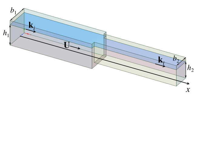
Figure 1: (Color online). Sketch of a canal consisting of two sections of different rectangular cross-sections. The wave number of incident wave is ${\bf k}_{i}$, and the wave number of transmitted wave is ${\bf k}_{t}$ (a reflected wave is not shown). Water flow $U$ is co-directed with the $x$-axis.

The Lamb model has been further generalised for waves of arbitrary wavelengths and applied to many practical problems. One of the typical applications of such a model is in the problem of oceanic wave transformation in the shelf zone; the numerous references can be found in the books and reviews (Massel, 1989; Dingemans, 1997; Kurkin et al., 2015). In such applications the canal width is assumed to be either constant or infinitely long and only the water depth abruptly changes.

A similar problem was studied also in application to internal waves, but analytical results were obtained only for the transformation coefficients of long waves in a two-layer fluid (Grimshaw et al., 2008), whereas for waves of arbitrary wavelength only the numerical results were obtained and the approximative formulae were suggested (Churaev et al., 2015).

All aforementioned problems of wave transformation were studied for cases when there is no background current. However, there are many situations when there is a flow over an underwater step or in the canals or rivers with variable cross-sections. The presence of a current can dramatically affect the transformation coefficients due to the specific wave-current interaction (see, e.g., Ref. (Belibassakis et al., 2011) and references therein). The amplitudes and energies of reflected and transmitted waves can significantly exceed the amplitude and energy of an incident wave. Such over-reflection and over-transmission phenomena are known in hydrodynamics and plasma physics (see, e.g., Ref. (Jones, 1968)); the wave energy in such cases can be extracted from the mean flow. Apparently, due to complexity of wave scattering problem in the presence of a background flow, no results were obtained thus far even for a relatively weak flow and small flow variation in a canal. There are, however, a number of works devoted to wave-current interactions and, in particular, wave scattering in spatially varying flows mainly on deep water (see, for instance, Refs. Smith (1975); Stiassnie and Dagan (1979); Trulsen and Mei (1993); Belibassakis et al. (2011) and references therein). In Ref. (Belibassakis et al., 2011) the authors considered the surface wave scattering in two-dimensional geometry in $(x,y)$-plane for the various models of underwater obstacles and currents including vortices. In particular, they studied numerically wave passage over an underwater step in the shoaling zone in the presence of a current. However, the transformation coefficients were not obtained even in the plane geometry.

Here we study the problem of long wave scattering analytically for all possible configurations of the background flow and incident wave (downstream and upstream propagation) in the narrowing or widening canal (accelerating or decelerating flow) for the subcritical, transcritical, and supercritical regimes when the current speed is less or greater than the typical wave speed $c_{0}=\sqrt{gh}$ in calm water in the corresponding canal section ($g$ is the acceleration due to gravity, and $h$ is the canal depth). Because we consider a limiting model case of very long waves when the variation of canal geometry is abrupt, the wave blocking phenomenon here has a specific character of reflection. Such a phenomenon has been studied in shallow-water limit in Ref. Smith (1975), but transformation coefficients were not obtained.

Notice also that in the last decade the problem of wave-current interaction in water with a spatially varying flow has attracted a great deal of attention from researchers due to application to the modelling of Hawking’s radiation emitted by evaporating black holes (Unruh, 1981) (see also Refs. (Jacobson, 1991; Unruh, 1995; Faccio et al., )). Recent experiments in a water tank (Euvé et al., 2016) have confirmed the main features of the Hawking radiation; however many interesting and important issues are still under investigation. In particular, it is topical to calculate the transformation coefficients of all possible modes generated in the process of incident mode conversion in the spatially varying flow. Several papers have been devoted to this problem both for the subcritical (Coutant and Weinfurtner, 2016; Robertson et al., 2016) and transcritical (Coutant et al., 2012; Robertson, 2012) flows. However, in all these papers the influence of wave dispersion was important, whereas there is no dispersion in the problem of black hole radiation. Our results for the dispersionless wave transformation can shed light on the problem of mode conversion in the relatively simple model considered in this paper.

II Problem statement and dispersion relation

Consider a long surface gravity wave propagating on the background current in a canal consisting of two portions of different cross-section each as shown in Fig. 1. A similar problem with a minor modification can be considered for internal waves in two-layer fluid, but we focus here on the simplest model to gain an insight in the complex problem of wave-current interaction. We assume that both the canal width and depth abruptly change at the same place, at the juncture of two canal portions. The current is assumed to be uniform across the canal cross-section and flows from left to right accelerating, if the canal cross-section decreases, or decelerating, if it increases. In the presence of a current the water surface does not remain plane even if the canal depth is unchanged, but the width changes. According to the Bernoulli law, when the current accelerates due to the canal narrowing, the pressure in the water decreases and, as a result, the level of the free surface reduces. Therefore, asymptotically, when $x\to\infty$, the portion of canal cross-section occupied by water is $S_{2}=b_{2}h_{2}$. A similar variation in the water surface occurs in any case when the current accelerates due to decrease of the canal cross-section in general; this is shown schematically in Fig. 2 (this figure is presented not in scale, just for the sake of a vivid explanation of the wave scattering, whereas in fact, we consider periodic waves with the wavelengths much greater than the fluid depth).

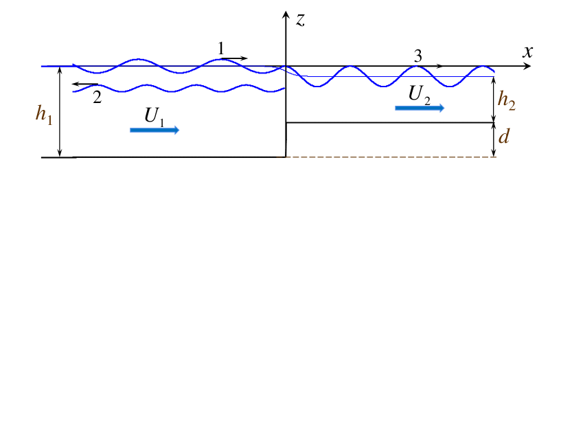
Figure 2: (Color online). The side view of a flow in a canal with a variable cross-section. Wave 1 schematically represents an incident wave, wave 2 – a reflected wave, and wave 3 – a transmitted wave. The water surface slightly lowers when the background flow increases as shown schematically by thin line.

The relationship between the water depth $h_{2}$, which asymptotically onsets at the infinity, and variations of canal width and depth at the juncture point is nontrivial. In particular, even in the case when the canal width is unchanged, and the canal cross-section changes only due to the presence of a bottom step of a height $d$, the water depth $h_{2}$ at the infinity is not equal to the difference $h_{1}-d$ (see, e.g., Ref. (Gazizov and Maklakov, 2004)). As shown in the cited paper, variation of a free surface due to increase of water flow is smooth even in the case of abruptly changed depth, but in the long-wave approximation it can be considered as abrupt. In any case, we will parameterize the formulas for the transformation coefficients in terms of the real depth ratio at plus and minus infinity $X=h_{2}/h_{1}$ and canal width aspect ratio $Y=b_{2}/b_{1}$. The long-wave approximation allows us to neglect the dispersion assuming that the wavelength $\lambda$ of any wave participating in the scattering is much greater than the canal depth $h$ in the corresponding section.

In the linear approximation the main set of hydrodynamic equations for shallow-water waves in a perfect incompressible fluid is (see, e.g., Ref. (Lamb, 1932)):

$$\frac{\partial u}{\partial t}+U\frac{\partial u}{\partial x} = -g\frac{\partial\eta}{\partial x},$$ (1)

$$\frac{\partial\eta}{\partial t}+U\frac{\partial\eta}{\partial x} = -h\frac{\partial u}{\partial x}.$$ (2)

Here $u(x,t)$ is a wave induced perturbation of a horizontal velocity, $U$ is the velocity of background flow which is equal to $U_{1}$ at minus infinity and $U_{2}$ at plus infinity, $\eta(x,t)$ is the perturbation of a free surface due to the wave motion, and $h$ is the canal depth which is equal to $h_{1}$ at minus infinity and $h_{2}$ at plus infinity – see Fig. 2.

For the incident harmonic wave of the form $\sim\mathrm{e}^{\mathrm{i}(\omega t-kx)}$ co-propagating with the background flow we obtain from Eq. (2)

$$\left(\omega-U_{1}k_{i}\right)\eta_{i}=h_{1}k_{i}u_{i},$$ (3)

where index $i$ pertains to incident wave (in what follows indices $t$ and $r$ will be used for the transmitted and reflected waves respectively).

Combining this with Eq. (1), we derive the dispersion relation for the incident wave

$$\omega=\left(U_{1}+c_{01}\right)k_{i},$$ (4)

where $c_{01}=\sqrt{gh_{1}}$.

Similarly for the transmitted wave we have $\left(\omega-U_{2}k_{t}\right)\eta_{t}=h_{2}k_{t}u_{t}$ and the dispersion relation $\omega=\left(U_{2}+c_{02}\right)k_{t}$, where $c_{02}=\sqrt{gh_{2}}$. Notice that the wave frequency remains unchanged in the process of wave transformation in a stationary, but spatially varying medium. Then, equating the frequencies for the incident and transmitted waves, we obtain $k_{t}/k_{i}=\left(U_{1}+c_{01}\right)/\left(U_{2}+c_{02}\right)$.

From the mass conservation for the background flow we have $U_{1}h_{1}b_{1}=U_{2}h_{2}b_{2}$ or $U_{1}/U_{2}=XY$. Using this relationship, we obtain for the wave number of the transmitted wave

$$\frac{k_{t}}{k_{i}}=XY\frac{1+\mathrm{Fr}}{X^{3/2}Y+\mathrm{Fr}},$$ (5)

where $\mathrm{Fr}=U_{1}/c_{01}$ is the Froude number.

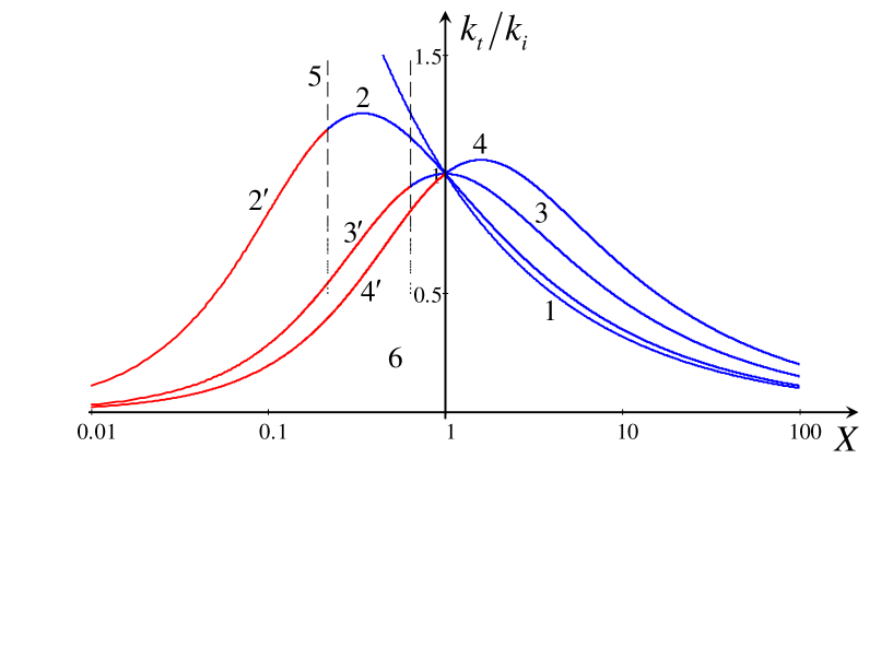
Figure 3: (Color online). The dependence of wave number ratio on the depth drop $X=h_{2}/h_{1}$ for different Froude numbers and $Y=1$. Line 1 pertains to the reference case when $\mathrm{Fr}=0$, lines 2 and $2^{\prime}$ – to $\mathrm{Fr}=0.1$, lines 3 and $3^{\prime}$ – to $\mathrm{Fr}=0.5$, line 4 and $4^{\prime}$ – to $\mathrm{Fr}=1$. Dashed vertical lines 5 and 6 show the boundaries between the subcritical and supercritical regimes in the downstream domain for $\mathrm{Fr}=0.1$, line 5, and $\mathrm{Fr}=0.5$, line 6.

The relationship between the wave numbers of incident and transmitted waves as functions of the depth drop $X$ is shown in Fig. 3 for several values of $\mathrm{Fr}$ and $Y=1$. As one can see, the ratio of wave numbers $k_{t}/k_{i}$ non-monotonically depends on $X$; it has a maximum at $X_{m}=\left(2\mathrm{Fr}/Y\right)^{2/3}$. The maximum value $\left(k_{t}/k_{i}\right)_{max}=\sqrt[3]{4Y}\left(1+\mathrm{Fr}\right)/\left(3\sqrt[3]{\mathrm{Fr}}\right)$ is also a non-monotonic function of the Froude number; it has a minimum at $\mathrm{Fr}=0.5$ where $\left(k_{t}/k_{i}\right)_{max}=\sqrt[3]{Y}$. In the limiting case, when there is no current ($\mathrm{Fr}=0$), $k_{t}/k_{i}=X^{-1/2}$ independently of $Y$ (see line 1 in Fig. 3). The current with the Froude number $\mathrm{Fr}<1$ remains subcritical in the downstream domain, if $X>\left(\mathrm{Fr}/Y\right)^{2/3}$. Otherwise it becomes supercritical. Dashed lines 5 and 6 in Fig. 3 show the boundaries between the subcritical and supercritical regimes in the downstream domains for two values of the Froude number, $\mathrm{Fr}=0.1$ and $\mathrm{Fr}=0.5$ respectively.

For the upstream propagating reflected wave the harmonic dependencies of free surface and velocity perturbations are $\{\eta,u\}\sim\mathrm{e}^{\mathrm{i}(\omega t+k_{r}x)}$. Then from Eq. (2) we obtain $\left(\omega+U_{1}k_{r}\right)\eta_{r}=-h_{1}k_{r}u_{r}$, and combining this with Eq. (1), we derive the dispersion relation for the reflected wave with $k_{r}<0$

$$\omega=\left(c_{01}-U_{1}\right)|k_{r}|.$$ (6)

Equating the frequencies of the incident and reflected waves, we obtain from the dispersion relations the relationship between the wave numbers:

$$\frac{|k_{r}|}{k_{i}}=\frac{1+\mathrm{Fr}}{1-\mathrm{Fr}}.$$ (7)

Notice that the ratio of wave numbers $|k_{r}|/k_{i}$ depends only on $\mathrm{Fr}$, but does not depend on $X$ and $Y$.

The dispersion relations for long surface waves on a constant current are shown in Fig. 4. Lines 1 and 2 show the dispersion dependencies for the downstream and upstream propagating waves, respectively, in the upstream domain, if the background current is subcritical, i.e., when $\mathrm{Fr}<1$. Lines 3 and 4 show the dispersion dependencies for the downstream and upstream propagating waves, respectively, which can potentially exist in the downstream domain, if the background current remains subcritical in this domain too, i.e. when $U_{2}/c_{02}\equiv\mathrm{Fr}/\left(X^{3/2}Y\right)<1$. If there is a source generating an incident wave of frequency $\omega$ and wave number $k_{i}$ at minus infinity, then after scattering at the canal juncture the reflected wave appears in the upstream domain with the same frequency and wave number $k_{r}$. Dashed horizontal line 7 in Fig. 4 shows the given frequency $\omega$. In the downstream domain with a subcritical flow the incident wave generates only one transmitted wave with the wave number $k_{t}$.

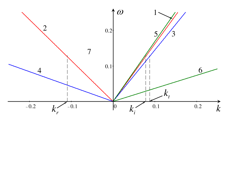
Figure 4: (Color online). Qualitative sketch of dispersion lines for long surface waves on a uniform background flow in a canal. For details see the text.

If the flow in one of the domains becomes faster and faster so that $\mathrm{Fr}\to 1_{-}$, then the dispersion line corresponding to the upstream propagating waves tilts to the negative portion of horizontal axis $k$ in Fig. 4 (cf. lines 2 and 4), and its intersection with the horizontal dashed line 7 shifts to the minus infinity. In the case of a supercritical flow, $\mathrm{Fr}>1$, the dispersion line corresponding to the upstream propagating waves is line 6 in Fig. 4. Its intersection with the horizontal dashed line 7 originates at the plus infinity (as the continuation of the intersection point of line 4 with line 7 disappeared at the minus infinity) and moves to the left when the flow velocity increases. The speeds of such waves in a calm water are smaller than the speed of a current, therefore despite the waves propagate counter current, the current traps them and pulls downstream. In the immovable laboratory coordinate frame they look like waves propagating to the right jointly with the current. As shown in Refs. (Stepanyants and Fabrikant, 1989; Fabrikant and Stepanyants, 1998; Maïssa et al., 2016a), such waves possess a negative energy. This means that the total energy of a medium when waves are excited is less then the energy of a medium without waves. Obviously, this can occur only in the non-equilibrium media, for example, in hydrodynamical flows possessing kinetic energy. In the equilibrium media, wave excitation makes the total energy greater than the energy of the non-perturbed media (more detailed discussion of the negative energy concept one can find in the citations presented above and references therein). In Appendix A we present the direct calculation of wave energy for the dispersionless case considered here and show when it become negative.

With the help of dispersion relations, the links between the perturbations of fluid velocity and free surface in the incident, reflected and transmitted waves can be presented as

$$u_{i}=c_{01}\eta_{i}/h_{1};\quad u_{r}=-c_{01}\eta_{r}/h_{1};\quad u_{t}=c_{02}\eta_{t}/h_{2}.$$ (8)

Using these relationships, we calculate in the next sections the transformation coefficients for all possible flow regimes and wave-current configurations.

III Subcritical flow in both the upstream and downstream domains

III.1 Downstream propagating incident wave

Consider first the case when the current is co-directed with the $x$-axis (see Fig. 2) and the incident wave travels in the same direction. Then, the transmitted wave is also co-directed with the current, but the reflected wave travels against the current. We assume that the current is subcritical in both left domain and right domains, i.e. its speed $U_{1}<c_{01}$ and $U_{2}<c_{02}$. This can be presented alternatively in terms of the Froude number and canal specific ratios, viz $\mathrm{Fr}<1$ and $\mathrm{Fr}<X^{3/2}Y$.

To derive the transformation coefficients, we use the boundary conditions at the juncture point $x=0$. These conditions physically imply the continuity of pressure and continuity of horizontal mass flux induced by a surface wave. The total pressure in the moving fluid consists of hydrostatic pressure $\rho g(h+\eta)$ and kinetic pressure $\rho(U+u)^{2}/2$. The condition of pressure continuity in the linear approximation reduces to

$$g\eta_{1}+U_{1}u_{1}=g\eta_{2}+U_{2}u_{2},$$ (9)

where indices 1 and 2 pertain to the left and right domains respectively far enough from the juncture point $x=0$. In the left domain we have $\{\eta_{1},u_{1}\}=\{\eta_{i}+\eta_{r},u_{i}+u_{r}\}$, whereas in the right domain $\{\eta_{2},u_{2}\}=\{\eta_{t},u_{t}\}$.

Using the relationships between $u_{i,r,t}$ and $\eta_{i,r,t}$ as per Eq. (8) and assuming that the incident wave has a unit amplitude in terms of $\eta$, we obtain from Eq. (9)

$$g\left(1+R_{\eta}\right)+U_{1}\frac{c_{01}}{h_{1}}\left(1-R_{\eta}\right)=gT_{\eta}+U_{2}\frac{c_{02}}{h_{2}}T_{\eta},$$ (10)

where $R_{\eta}$ and $T_{\eta}$ are amplitudes of reflected and transmitted waves respectively. In the dimensionless form this equations reads

$$1+\mathrm{Fr}+\left(1-\mathrm{Fr}\right)R_{\eta}=T_{\eta}\left(1+\frac{\mathrm{Fr}}{X^{3/2}Y}\right).$$ (11)

The condition of mass flux continuity leads to the equation

$$\rho b_{1}\left(h_{1}+\eta_{1}\right)\left(U_{1}+u_{1}\right)=\rho b_{2}\left(h_{2}+\eta_{2}\right)\left(U_{2}+u_{2}\right).$$ (12)

In the linear approximation and dimensionless form this gives:

$$1+\mathrm{Fr}-\left(1-\mathrm{Fr}\right)R_{\eta}=T_{\eta}\sqrt{X}Y\left(1+\frac{\mathrm{Fr}}{X^{3/2}Y}\right).$$ (13)

After that we derive the transformation coefficients $R_{\eta}$ and $T_{\eta}$ from Eqs. (11) and (13):

$$R_{\eta}=\frac{1+\mathrm{Fr}}{1-\mathrm{Fr}}\frac{1-\sqrt{X}Y}{1+\sqrt{X}Y},\quad T_{\eta}=\frac{1+\mathrm{Fr}}{X^{3/2}Y+\mathrm{Fr}}\frac{2X^{3/2}Y}{1+\sqrt{X}Y}.$$ (14)

These formulas naturally reduce to the well-known Lamb formulas (Lamb, 1932) when $\mathrm{Fr}\to 0$. Graphics of $T_{\eta}$ and $R_{\eta}$ as functions of depth drop $X$ are shown in Fig. 5 for the particular value of Froude number $\mathrm{Fr}=0.5$ and $Y=1$.

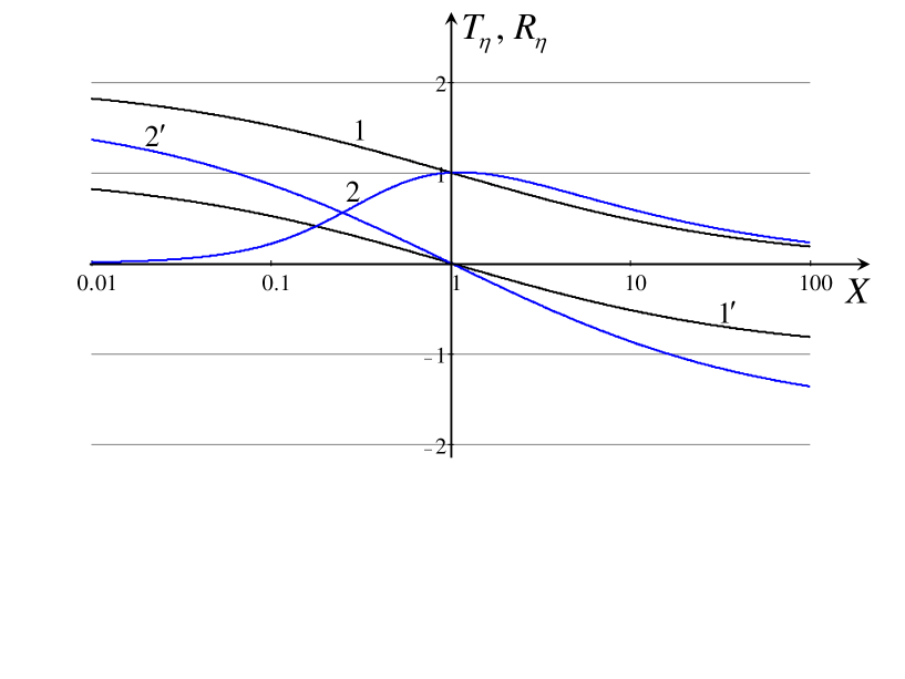
Figure 5: (Color online). The transformation coefficients of surface waves on a uniform subcritical current in a canal with flat walls, $Y=1$, as functions of the depth drop $X$. Line 1 for $T_{\eta}$ and line $1^{\prime}$ for $R_{\eta}$ pertain to the reference case given by the Lamb formulas with $\mathrm{Fr}=0$; lines 2 (for $T_{\eta}$) and $2^{\prime}$ (for $R_{\eta}$) pertain to the flow with $\mathrm{Fr}=0.5$.

As follows from the formula for $R_{\eta}$, the reflection coefficient increases uniformly in absolute value, when the Froude number increases from 0 to 1, provided that $\sqrt{X}Y\neq 1$. It is important to notice that the reflectionless propagation can occur in the case, when $\sqrt{X}Y=1$, whereas neither $X$, nor $Y$ are equal to one. The transmission coefficient in this case $T_{\eta}=\left(1+\mathrm{Fr}\right)/\left(1+Y^{2}\mathrm{Fr}\right)\neq 1$ in general, except the case when $\mathrm{Fr}=0$. The reflection coefficient is negative when $\sqrt{X}Y>1$, which means that the reflected wave is in anti-phase with respect to the incident wave.

The dependence of $T_{\eta}$ on the Froude number is more complicated and non-monotonic in $X$. However, in general $T_{\eta}\to 0$ in two limiting cases, when $X\to 0$, then $T_{\eta}\approx 2X^{3/2}Y\left(1+1/\mathrm{Fr}\right)$, and when $X\to\infty$, then $T_{\eta}\approx 2\left(1+\mathrm{Fr}\right)/\left(\sqrt{X}Y\right)$ (see Fig. 5).

It is appropriate to mention here the nature of singularity of the reflection coefficient $R_{\eta}$ and wave number $k_{r}$ of the reflected wave as per Eq. (7) when $\mathrm{Fr}\to 1$. In such case, the dispersion line 2 in Fig. 4 approaches negative half-axis of $k$, and the point of intersection of line 2 with the dashed horizontal line 7 shifts to the minus infinity, i.e. $k_{r}\to-\infty$, and the wavelength of reflected wave $\lambda_{r}=2\pi/|k_{r}|\to 0$. Thus, we see that when $\mathrm{Fr}\to 1$, then the amplitude of the reflected wave $R_{\eta}$ infinitely increases, and its wavelength vanishes. It will be shown below that the wave energy flux associated with the reflected wave remains finite even when $\mathrm{Fr}=1$.

The results obtained for the transformation coefficients are in consistency with the wave energy flux conservation in an inhomogeneous stationary moving fluid (see, e.g., Ref. (Longuet-Higgins, 1996)), $W\equiv V_{g}E=\mathrm{const.}$, where $V_{g}\equiv d\omega/dk$ is the group speed in the moving fluid, and $E$ is the density of wave energy. In the case of long waves in shallow water we have $\left(V_{g}\right)_{1,2}=\left(c_{0}\right)_{1,2}\pm U_{1,2}$. As shown in Appendix A (see also Refs. (Dysthe, 2004; Maïssa et al., 2016a)), the period-averaged energy density in the long-wave limit is $E=gA^{2}b\left(1\pm\mathrm{Fr}\right)/2$, where $A$ is the amplitude of free surface perturbation, $b$ is the canal width, sign plus pertains to waves co-propagating with the background flow, and sign minus – to waves propagating against the flow. Taking into account that the energy fluxes in the incident and transmitted waves are directed to the right, and the energy flux in the reflected wave is directed to the left, we obtain

$$\left(1+\mathrm{Fr}\right)^{2}-\left(1-\mathrm{Fr}\right)^{2}R_{\eta}^{2}=\sqrt{X}Y\left(1+\frac{\mathrm{Fr}}{X^{3/2}Y}\right)^{2}T_{\eta}^{2},$$ (15)

where the factor $\sqrt{X}Y$ accounts for the change of the cross-sectional area of the canal.

Substituting here the expressions for the transformation coefficients Eq. (14), we confirm that Eq. (15) reduces to the identity. Notice that the second term in the left-hand side of Eq. (15), which represents the energy flux induced by the reflected wave, remains finite even at $\mathrm{Fr}=1$.

The gain of energy densities in the reflected and transmitted waves can be presented as the ratios $E_{r}/E_{i}$ and $E_{t}/E_{i}$. Using the formulas for the transformation coefficients and expression for the wave energy in a moving fluid (see above), we obtain

$$\frac{E_{r}}{E_{i}}=\frac{1+\mathrm{Fr}}{1-\mathrm{Fr}}\left(\frac{1-\sqrt{X}Y}{1+\sqrt{X}Y}\right)^{2},\quad\frac{E_{t}}{E_{i}}=\frac{4Y}{\left(1+\sqrt{X}Y\right)^{2}}\frac{1+\mathrm{Fr}}{1+\mathrm{Fr}/X^{3/2}Y}.$$ (16)

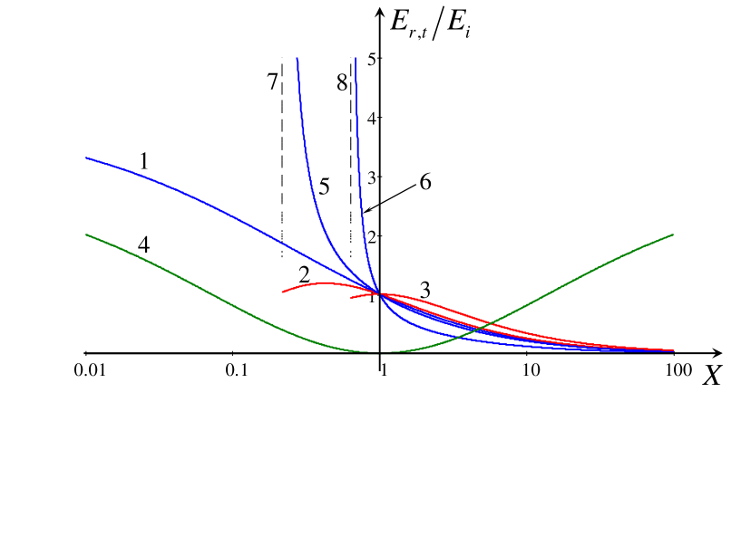
Figure 6: (Color online). The gain of energy density in the transmitted wave for several Froude numbers and $Y=1$ as functions of the depth drop $X$. Line 1 pertains to the reference case when $\mathrm{Fr}=0$; lines 2 and 3 pertain to the downstream propagating waves in the subcritical flows with $\mathrm{Fr}=0.1$ and 0.5 respectively; and lines 5 and 6 pertain to the upstream propagating waves in the same flows. Line 4 shows the typical dependence of energy density gain in the upstream propagating reflected wave with $\mathrm{Fr}=0.5$. Lines 7 and 8 show the boundaries of subcritical regimes for $\mathrm{Fr}=0.1$ and 0.5 respectively.

As follows from the first of these expressions, the density of wave energy in the reflected wave is enhanced uniformly by the current at any Froude number ranging from 0 to 1 regardless of $X$ and $Y$, whereas the density of wave energy in the transmitted wave can be slightly enhanced by the current only if $X^{3/2}Y>1$; otherwise, it is less than that in the incident wave. Figure 6 illustrates the gain of energy density in the transmitted wave for several Froude numbers and $Y=1$. Line 4 in that figure shows the typical dependence of $E_{r}/E_{i}$ on $X$ for $\mathrm{Fr}=0.5$ and $Y=1$. When $\mathrm{Fr}\to 1$ the gain of wave energy in the reflected wave infinitely increases within the framework of a linear model considered here (in reality the nonlinear, viscous, or dispersive effects can restrict infinite growth). In this case the typical over-reflection phenomenon (Jones, 1968) occurs in the scattering of downstream propagating wave, when the energy density in the reflected wave becomes greater than the energy density in the incident wave. This can occur due to the wave energy extraction from the mean flow.

III.2 Upstream propagating incident wave

Consider now the case when the current is still co-directed with the $x$ axis (see Fig. 2) and the incident wave travels in the opposite direction from plus infinity. Then, the transmitted wave in the left domain propagates counter current, and the reflected wave in the right domain is co-directed with the current. In the dispersion diagram shown in Fig. 4 the incident wave now corresponds to the intersection of line 2 with the dashed horizontal line 7 (with the wave number $k_{r}$ replaced by $k_{i}$), the reflected wave corresponds to intersection of line 1 with line 7 (with the wave number $k_{i}$ replaced by $k_{r}$), and the transmitted wave corresponds to the intersection of line 4 with line 7 (not visible in the figure).

To derive the transformation coefficients, we use the same boundary conditions at the juncture point $x=0$ and after simple manipulations similar to those presented in the previous subsection we obtain essentially the same formulas for the wave numbers of transmitted and reflected waves as in Eqs. (5) and (7), as well as the transformation coefficients as in Eqs. (14) with the only difference that the sign of the Froude number should be changed everywhere to the opposite, $\mathrm{Fr}\to-\mathrm{Fr}$. However, the change of sign in the Froude number leads to singularities in both the wave number of the transmitted wave and the transmission coefficient. Therefore for the wave numbers of scattered waves we obtain:

$$\frac{k_{r}}{k_{i}}=\frac{1-\mathrm{Fr}}{1+\mathrm{Fr}},\quad\frac{k_{t}}{k_{i}}=XY\frac{1-\mathrm{Fr}}{X^{3/2}Y-\mathrm{Fr}}.$$ (17)

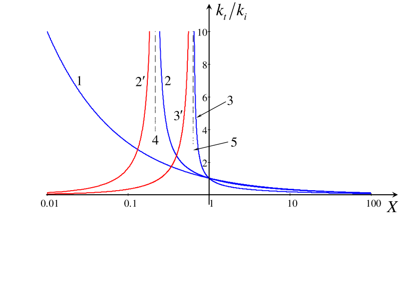
Figure 7: (Color online). The dependences of normalized wave numbers of transmitted waves on the depth drop $X$ for $Y=1$ and several particular values of the Froude number. Line 1 pertains to the reference case when there is no flow ($\mathrm{Fr}=0$); other lines pertain to the subcritical cases (line 2 – $\mathrm{Fr}=0.1$; line 3 – $\mathrm{Fr}=0.5$) and supercritical cases (line $2^{\prime}$ – $\mathrm{Fr}=0.1$; line $3^{\prime}$ – $\mathrm{Fr}=0.5$). Dashed vertical lines 4 and 5 show the boundaries between the subcritical and supercritical cases for $\mathrm{Fr}=0.1$ and 0.5, respectively.

In Fig. 7, lines 1 – 3 show the dependencies of normalized wave numbers of transmitted waves on the depth drop $X$ for $Y=1$ and several particular values of the Froude number. Line 1 pertains to the reference case studied by Lamb (1932) when there is no flow ($\mathrm{Fr}=0$). As one can see, when the depth drop decreases and approaches the critical value, $X\to X_{c}=\left(\mathrm{Fr}/Y\right)^{2/3}$, the wave number of the transmitted wave becomes infinitely big (and the corresponding wavelength vanishes). This means that the current in the left domain becomes very strong and supercritical; the transmitted wave cannot propagate against it and the blocking phenomenon occurs (see, e.g., Refs. (Basovich and Talanov, 1977; Maïssa et al., 2016b) and references therein).

The transformation coefficients for this case are

$$R_{\eta}=\frac{1-\mathrm{Fr}}{1+\mathrm{Fr}}\frac{1-\sqrt{X}Y}{1+\sqrt{X}Y},\quad T_{\eta}=\frac{1-\mathrm{Fr}}{X^{3/2}Y-\mathrm{Fr}}\frac{2X^{3/2}Y}{1+\sqrt{X}Y}.$$ (18)

They are as shown in Fig. 8 in the domains where the subcritical regime occurs, $X>\left(\mathrm{Fr}/Y\right)^{2/3}$ as the functions of depth drop $X$ for $Y=1$ and two values of the Froude number. When depth drop decreases and approaches the critical value $X_{c}$, the transmission coefficient infinitely increases, and the over-transmission phenomenon occurs. However, it can be readily shown that the energy flux remains finite, and the law of energy flux conservation Eq. (15) with $\mathrm{Fr}\to-\mathrm{Fr}$ holds true in this case too.

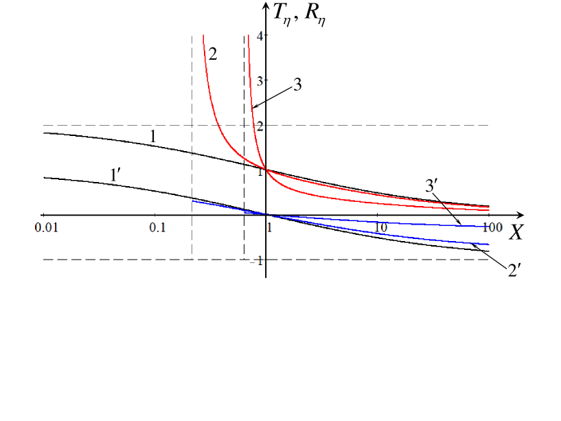
Figure 8: (Color online). The transformation coefficients for the upstream propagating incident waves in a canal with flat walls, $Y=1$, as functions of depth drop $X$. Line 1 for $T_{\eta}$ and line $1^{\prime}$ for $R_{\eta}$ pertain to the reference case when $\mathrm{Fr}=0$; lines 2 (for $T_{\eta}$) and $2^{\prime}$ (for $R_{\eta}$) pertain to $\mathrm{Fr}=0.1$, and lines 3 (for $T_{\eta}$) and $3^{\prime}$ (for $R_{\eta}$) pertain to $\mathrm{Fr}=0.5$.

The gain of energy densities in the reflected and transmitted waves follows from Eq. (16) if we replace $\mathrm{Fr}$ by $-\mathrm{Fr}$ (see lines 4 and 5 in Fig. 6):

$$\frac{E_{r}}{E_{i}}=\frac{1-\mathrm{Fr}}{1+\mathrm{Fr}}\left(\frac{1-\sqrt{X}Y}{1+\sqrt{X}Y}\right)^{2},\quad\frac{E_{t}}{E_{i}}=\frac{4Y}{\left(1+\sqrt{X}Y\right)^{2}}\frac{1-\mathrm{Fr}}{1-\mathrm{Fr}/X^{3/2}Y}.$$ (19)

The presence of a subcritical current leads to uniform decrease of wave energy density in the reflected wave regardless of $X$ and $Y$. Moreover, the wave density in this wave vanishes when $\mathrm{Fr}\to 1$. However, in the transmitted wave the density of wave energy quickly increases when $X\to X_{c}$ being greater than $X_{c}$ (see lines 5 and 6 in Fig. 6). Thus, the typical over-transmission phenomenon occurs in the scattering of upstream propagating wave (cf. with the over-reflection phenomenon described at the end of the previous subsection).

IV Subcritical flow in the upstream domain, but supercritical in the downstream domain

In such a case an incident wave can propagate only along the current. In the downstream domain where the current is supercritical no one wave can propagate against it. Therefore, we consider here a scattering of only a downstream propagating incident wave which arrives from minus infinity in Fig. 1. We assume that the Froude number and geometric parameters of a canal are such that $X^{3/2}Y<\mathrm{Fr}<1$.

In the upstream domain two waves of frequency $\omega$ can propagate in the subcritical flow. One of them is an incident wave with the unit amplitude and wave number $k_{i}=\omega/(c_{01}+U_{1})$ and another one is the reflected wave with the amplitude $R_{\eta}$ and wave number $k_{r}=\omega/(c_{01}-U_{1})$. In the downstream domain two waves can exist too. One of them is the transmitted wave of positive energy with the amplitude $T_{p}$ and wave number $k_{t1}=\omega/(U_{2}+c_{02})$ and another one is the transmitted wave of negative energy (see the Appendix) with the amplitude $T_{n}$ and wave number $k_{t2}=\omega/(U_{2}-c_{02})$.

The relationships between the wave numbers of scattered waves follows from the frequency conservation. For the transmitted wave of positive energy and reflected wave we obtain the same formulas as in Eqs. (5) and (7), whereas for the transmitted wave of negative energy we obtain

$$\frac{k_{t2}}{k_{i}}=XY\frac{\mathrm{Fr}+1}{\mathrm{Fr}-X^{3/2}Y}.$$ (20)

As follows from this formula, the wave number $k_{t2}$ infinitely increases when $X\to X_{c}$ being less than $X_{c}$. The dependencies of $k_{t1}/{k_{i}}$ are shown in Fig. 3 by lines $2^{\prime}$, $3^{\prime}$, and $4^{\prime}$ for $\mathrm{Fr}=0.1,\;0.5$, and 1, respectively, whereas the dependencies of $k_{t2}/{k_{i}}$ are shown in Fig. 7 by lines $2^{\prime}$ and $3^{\prime}$ for $\mathrm{Fr}=0.1$ and 0.5 respectively.

To find the transformation coefficients we use the same boundary conditions as in Eqs. (10) and (12), but now they provide the following set of equations:

$$1+\mathrm{Fr}+\left(1-\mathrm{Fr}\right)R_{\eta} = T_{p}\left(1+\frac{\mathrm{Fr}}{X^{3/2}Y}\right)+T_{n}\left(1-\frac{\mathrm{Fr}}{X^{3/2}Y}\right),$$ (21)

$$1+\mathrm{Fr}-\left(1-\mathrm{Fr}\right)R_{\eta} = \sqrt{X}Y\left[T_{p}\left(1+\frac{\mathrm{Fr}}{X^{3/2}Y}\right)-T_{n}\left(1-\frac{\mathrm{Fr}}{X^{3/2}Y}\right)\right].$$ (22)

This set relates three unknown quantities, $R_{\eta}$, $T_{p}$, and $T_{n}$. We can express, for example, amplitudes of transmitted waves $T_{p}$ and $T_{n}$ in terms of unit amplitude of incident wave and amplitude of reflected wave $R_{\eta}$:

$$T_{p} = \frac{X}{2\left(X^{3/2}Y+\mathrm{Fr}\right)}\left[\left(1+\mathrm{Fr}\right)\left(\sqrt{X}Y+1\right)+\left(1-\mathrm{Fr}\right)\left(\sqrt{X}Y-1\right)R_{\eta}\right],$$ (23)

$$T_{n} = \frac{X}{2\left(X^{3/2}Y-\mathrm{Fr}\right)}\left[\left(1+\mathrm{Fr}\right)\left(\sqrt{X}Y-1\right)+\left(1-\mathrm{Fr}\right)\left(\sqrt{X}Y+1\right)R_{\eta}\right],$$ (24)

whereas the reflection coefficient $R_{\eta}$ remains unknown.

It can be noticed a particular case when the background flow could, probably, spontaneously generate waves to the both sides of a juncture where the background flow abruptly changes from the subcritical to supercritical value. Bearing in mind that the transformation coefficients are normalized on the amplitude of an incident wave, $R_{\eta}\equiv A_{r}/A_{i}$, $T_{p}\equiv A_{p}/A_{i}$, $T_{n}\equiv A_{n}/A_{i}$, and considering a limit when $A_{i}\to 0$, we obtain from Eqs. (23) and (24):

$$\frac{A_{r}}{A_{p}}=\frac{2}{X\left(1-\mathrm{Fr}\right)}\frac{X^{3/2}+\mathrm{Fr}}{\sqrt{X}Y-1},\quad\frac{A_{n}}{A_{p}}=\frac{\sqrt{X}Y+1}{\sqrt{X}Y-1}\frac{X^{3/2}+\mathrm{Fr}}{X^{3/2}-\mathrm{Fr}}.$$ (25)

The conservation of wave energy flux in general is

$$\left(1+\mathrm{Fr}\right)^{2}-\left(1-\mathrm{Fr}\right)^{2}R_{\eta}^{2}=\frac{1}{X^{5/2}Y}\left[\left(X^{3/2}Y+\mathrm{Fr}\right)^{2}T_{p}^{2}-\left(X^{3/2}Y-\mathrm{Fr}\right)^{2}T_{n}^{2}\right].$$ (26)

After substitution here of the transmission coefficients Eqs. (23) and (24) we obtain the identity regardless of $R_{\eta}$. In the case of spontaneous wave generation when there is no incident wave, Eq. (26) turns to the identity too after its re-normalization and substitution of Eqs. (25). This resembles a spontaneous wave generation due to Hawking’s effect (Unruh, 1981, 1995; Faccio et al., )) at the horizon of an evaporating black hole, when a positive energy wave propagates towards our space (the upstream propagating wave $A_{r}$ in our case), whereas a negative energy wave together with a positive energy wave propagates towards the black hole (the downstream propagating waves $A_{n}$ and $A_{p}$).

Thus, within the model with an abrupt change of canal cross-section the complete solution for the wave scattering cannot be obtained in general. One needs to discard from the approximation when the current speed abruptly increases at the juncture and consider a smooth current transition from one value $U_{1}$ to another one $U_{2}$ (this problem was recently studied in Ref. (Churilov et al., 2017)).

V Supercritical flow in both the upstream and downstream domains

Now let us consider a wave scattering in the case when the flow is supercritical both in upstream and downstream domain, $U_{1}>c_{01}$ and $U_{2}>c_{02}$. In terms of the Froude number we have $\mathrm{Fr}>1$ and $\mathrm{Fr}>X^{3/2}Y$. It is clear that in such a situation, similar to the previous subsection, only a downstream propagating incident wave can be considered.

In the upstream supercritical flow there is no reflected wave. In the dispersion diagram of Fig. 4 the downstream propagating incident wave of frequency $\omega$ can be either the wave on the intersection of line 5 with the dashed horizontal line, or on the intersection of line 6 with the dashed horizontal line (the intersection point is off the figure), or even both. The former wave is the wave of positive energy and has the wave number $k_{i1}=\omega/(U_{1}+c_{01})$, whereas the latter is the wave of negative energy (see the Appendix) and has the wave number $k_{i2}=\omega/(U_{1}-c_{01})$.

In the downstream domain where we assume that the flow is supercritical too, two waves appear as the result of scattering of incident waves. As in the upstream domain, one of the transmitted waves has positive energy and the wave number $k_{t1}=\omega/(U_{2}+c_{02})$, and the other has negative energy and the wave number $k_{t2}=\omega/(U_{2}-c_{02})$.

Let us assume that there is a wavemaker at minus infinity that generates a sinusoidal surface perturbation of frequency $\omega$. Then, two waves of positive and negative energies with the amplitudes $A_{p}$ and $A_{n}$, respectively, can jointly propagate. In the process of wave scattering at the canal juncture two transmitted waves with opposite energies will appear with the amplitudes $T_{p}$ and $T_{n}$. Their amplitudes can be found from the boundary conditions Eqs. (10) and (12). Then, after simple manipulations similar to those in Secs. III and IV we obtain:

$$T_{p} = \frac{X}{2\left(X^{3/2}Y+\mathrm{Fr}\right)}\left[\left(\mathrm{Fr+1}\right)\left(\sqrt{X}Y+1\right)A_{p}-\left(\mathrm{Fr}-1\right)\left(\sqrt{X}Y-1\right)A_{n}\right],$$ (27)

$$T_{n} = \frac{X}{2\left(X^{3/2}Y-\mathrm{Fr}\right)}\left[\left(\mathrm{Fr+1}\right)\left(\sqrt{X}Y-1\right)A_{p}-\left(\mathrm{Fr}-1\right)\left(\sqrt{X}Y+1\right)A_{n}\right].$$ (28)

At certain relationships between the amplitudes $A_{p}$ and $A_{n}$ it may happen that there is only one transmitted wave, either of positive energy ($T_{n}=0$), when

$$A_{n}=A_{p}\frac{\mathrm{Fr}+1}{\mathrm{Fr}-1}\frac{\sqrt{X}Y-1}{\sqrt{X}Y+1},$$ (29)

or of negative energy ($T_{p}=0$), when

$$A_{n}=A_{p}\frac{\mathrm{Fr}+1}{\mathrm{Fr}-1}\frac{\sqrt{X}Y+1}{\sqrt{X}Y-1}.$$ (30)

From the law of wave energy flux conservation we obtain

$$\left(\mathrm{Fr}+1\right)^{2}A_{p}^{2}-\left(\mathrm{Fr}-1\right)^{2}A_{n}^{2}=\sqrt{X}Y\left[\left(\frac{\mathrm{Fr}}{X^{3/2}Y}+1\right)^{2}T_{p}^{2}-\left(\frac{\mathrm{Fr}}{X^{3/2}Y}-1\right)^{2}T_{n}^{2}\right].$$ (31)

Substituting here the expressions for $T_{p}$ and $T_{n}$ as per Eqs. (27) and (28), we see that Eq. (31) becomes an identity regardless of amplitudes of incoming waves $A_{p}$ and $A_{n}$, including the cases when they are related by Eqs. (29) or (30). In the particular cases one of the incident waves can be suppressed, ether the wave of negative energy or wave of positive energy. In the former case we set $A_{n}=0$ and $A_{p}=1$, and in the latter case we set $A_{p}=0$ and $A_{n}=1$.

When there is only one incident wave of positive energy with the amplitude $A_{p}=1$ and there is no wave of negative energy ($A_{n}=0$), then the transmission coefficients Eqs. (27) and (28) reduce to

$$T_{p}=\frac{X}{2}\frac{\mathrm{Fr}+1}{\mathrm{Fr}+X^{3/2}Y}\left(1+\sqrt{X}Y\right),\quad T_{n}=\frac{X}{2}\frac{\mathrm{Fr}+1}{\mathrm{Fr}-X^{3/2}Y}\left(1-\sqrt{X}Y\right).$$ (32)

Recall that these formulas are valid for supercritical flows when $\mathrm{Fr}>1$ and $\mathrm{Fr}>X^{3/2}Y$. In the limiting case when $X\to 0$ and $Y=\mathrm{const.}$, we obtain

$$T_{p}\approx T_{n}\approx X\frac{\mathrm{Fr}+1}{\mathrm{2Fr}}.$$ (33)

In another limiting case when $X^{3/2}Y\to\mathrm{Fr}$ the transmission coefficient for the positive energy wave remains constant, whereas the transmission coefficient for the negative energy wave within the framework of linear theory goes to plus or minus infinity depending on the value of $Y$. Figure 9(a) illustrates the transmission coefficients $T_{p}$ and $T_{n}$ as functions of $X$ for $Y=1$ and two particular values of the Froude number.

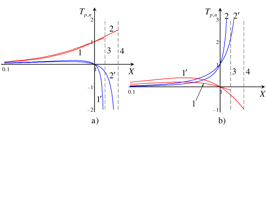
Figure 9: (Color online). The transmission coefficients for the downstream propagating incident waves of positive energy (frame a) and negative energy (frame b) in a canal with the flat walls, $Y=1$, as functions of the depth drop $X$. Line 1 for $T_{p}$ and line $1^{\prime}$ for $T_{n}$ pertain to $\mathrm{Fr}=1.5$, and lines 2 (for $T_{p}$) and $2^{\prime}$ (for $T_{n}$) pertain to $\mathrm{Fr}=2.5$. Data for lines 1 and 2 in frame (b) were multiplied by a factor of ten to make the graphics clearly visible.

When there is only one incident wave of negative energy with the amplitude $A_{n}=1$ and there is no wave of positive energy ($A_{p}=0$), then the transmission coefficients Eqs. (27) and (28) reduce to

$$T_{p}=\frac{X}{2}\frac{\mathrm{Fr}-1}{\mathrm{Fr}+X^{3/2}Y}\left(1-\sqrt{X}Y\right),\quad T_{n}=\frac{X}{2}\frac{\mathrm{Fr}-1}{\mathrm{Fr}-X^{3/2}Y}\left(1+\sqrt{X}Y\right).$$ (34)

In the limiting case when $X\to 0$, and $Y=\mathrm{const.}$, we obtain

$$T_{p}\approx T_{n}\approx X\frac{\mathrm{Fr}-1}{2\mathrm{Fr}}.$$ (35)

In another limiting case when $X^{3/2}Y\to\mathrm{Fr}$, the transmission coefficient for the positive energy wave remains finite, whereas, the transmission coefficient for the negative energy wave within the framework of linear theory goes to plus infinity. Figure 9(b) shows the transmission coefficients $T_{p}$ and $T_{n}$ as functions of $X$ for $Y=1$ for two particular values of the Froude number.

VI Supercritical flow in the upstream and subcritical in the downstream domain

Let us consider, at last, the case when the flow is supercritical in the upstream domain, where $U_{1}>c_{01}$, but due to canal widening becomes subcritical in the downstream domain, where $U_{2}<c_{02}$. Thus, the flow is decelerating and in terms of the Froude number we have $1<\mathrm{Fr}<X^{3/2}Y$. Assume first that the incident wave propagates downstream.

VI.1 Downstream propagating incident wave

As was mentioned in the previous section, two waves with the amplitudes $A_{p}$ and $A_{n}$ can propagate simultaneously from minus infinity, if they are generated by the same wavemaker with the frequency $\omega$. In the downstream domain potentially two waves of positive energy can exist, but only one of them propagating downstream can appear as the transmitted wave with the amplitude $T_{\eta}$ as the result of wave scattering at the juncture.

The amplitudes of scattered waves can be found from the boundary conditions Eqs. (10) and (12). This gives, after simple manipulations:

$$\left(1+\mathrm{Fr}\right)A_{p}+\left(1-\mathrm{Fr}\right)A_{n} = T_{\eta}\left(1+\frac{\mathrm{Fr}}{X^{3/2}Y}\right),$$ (36)

$$\left(1+\mathrm{Fr}\right)A_{p}-\left(1-\mathrm{Fr}\right)A_{n} = \sqrt{X}YT_{\eta}\left(1+\frac{\mathrm{Fr}}{X^{3/2}Y}\right).$$ (37)

This set of equations provides a unique solution for the transmission coefficient $T_{\eta}$ only in the case when the amplitudes of incoming waves are related:

$$A_{n}=\frac{1+\mathrm{Fr}}{1-\mathrm{Fr}}\frac{1-\sqrt{X}Y}{1+\sqrt{X}Y}A_{p},\quad T_{\eta}=\frac{1+\mathrm{Fr}}{X^{3/2}Y+\mathrm{Fr}}\frac{2X^{3/2}Y}{1+\sqrt{X}Y}A_{p}.$$ (38)

If one of the incident waves is absent ($A_{n}=0$ or $A_{p}=0$) or amplitudes of incoming waves are not related by Eq. (38), then the set of Eqs. (36) and (37) is inconsistent. In such cases the problem of wave scattering in the canal does not have a solution within the framework of a model with a sharp change of the cross-section.

If the amplitudes of incident waves $A_{p}$ and $A_{n}$ are related by Eq. (38), then the conservation of wave energy flux holds and takes the form

$$\left(\mathrm{Fr}+1\right)^{2}A_{p}^{2}-\left(\mathrm{Fr}-1\right)^{2}A_{n}^{2}=\sqrt{X}Y\left(\frac{\mathrm{Fr}}{X^{3/2}Y}+1\right)^{2}T_{\eta}^{2}.$$ (39)

Substituting here $A_{n}$ and $T_{\eta}$ from Eq. (38), we see that it becomes just the identity.

VI.2 Upstream propagating incident wave

For the incident wave arriving from the plus infinity and propagating upstream in the subcritical domain of the flow, the problem of wave scattering within the model with a sharp change of a current is undefined. The incoming wave cannot penetrate from the domain with a subcritical flow into the domain with a supercritical flow, therefore one can say that formally the reflection coefficient in this case $R_{\eta}=1$, and the transmission coefficients $T_{\eta}=0$. However such a problem should be considered within a more complicated model with a smooth transcritical flow; this has been done in Ref. (Churilov et al., 2017).

VII Conclusion

In this paper within the linear approximation we have studied a scattering of long surface waves at the canal juncture when its width and depth abruptly change at a certain place. We have calculated the transformation coefficients for the reflected and transmitted waves in the presence of a background flow whose speed changes from $U_{1}$ to $U_{2}$ in accordance with the mass flux conservation. The calculated coefficients represent the effectiveness of the conversion of the incident wave into the other wave modes – reflected and transmitted of either positive or negative energy. Our consideration generalizes the classical problem studied by Ref. Lamb (1932) when the background flow is absent. It was assumed that the characteristic scale of current variation in space is much less than the wavelengths of scattered waves. Such a simplified model allows one to gain insight into the complex problem of wave-current interaction and find the conditions for the over-reflection and over-transmission of water waves. We have analyzed all possible orientations of the incident wave with respect to flow and studied all possible regimes of water flow (subcritical, supercritical, and transcritical).

In the study of the subcritical and supercritical flows (see Secs. III and V) we have succeeded in calculating the transmission and reflection coefficients in the explicit forms as functions of the depth drop $X=h_{2}/h_{1}$, specific width ratio $Y=b_{2}/b_{1}$, and Froude number $\mathrm{Fr}$. Based on these, the conditions for the over-reflection and over-transmission have been found in terms of the relationships between the Froude number and canal geometric parameters $X$ and $Y$. It appears that it is not possible to do the same for the transcritical flows, at least within the framework of the simplified model considered in this paper (see Secs. IV and VI). The reason for that is in the critical point where $\mathrm{Fr}=1$ which appears in the smooth transient domain between two portions of a canal with the different cross-sections. The transition through the critical point is a rather complex problem which was recently studied on the basis of a model with a continuously varying flow speed in a duct of smoothly varying width (Churilov et al., 2017). The summary of results obtained is presented in Table I.

Table I. The summary of considered cases. A cocurrent propagating incident waves is denoted by $k_{i}\uparrow\uparrow U$, whereas a countercurrent propagating incident waves is denoted by $k_{i}\downarrow\uparrow U$. The acronyms PEW and NEW pertain to positive and negative energy waves, correspondingly.

I. Subcritical flow in the upstream and downstream domains
${\bf k}_{i}$, ${\bf U}$	Reflect. coeff.	Transmiss. coeff.	Peculiarity of a scattering
$k_{i}\uparrow\uparrow U$	$R_{\eta}$ see Eq. (14)	$T_{\eta}$ see Eq. (14)	Regular scattering
$k_{i}\downarrow\uparrow U$	$R_{\eta}$ see Eq. (18)	$T_{\eta}$ see Eq. (18)	Regular scattering
II. Subcritical flow in the upstream domain and supercritical in the
downstream domain. PEW and NEW appear downstream.
${\bf k}_{i}$, ${\bf U}$	Reflect. coeff.	Transmiss. coeff.	Peculiarity of a scattering
$k_{i}\uparrow\uparrow U$	$R_{\eta}$ is undetermined,	$T_{p}$ see Eq. (23)	Undefined problem statement,
	according to (Churilov et al., 2017), $R_{\eta}=1$	$T_{n}$ see Eq. (24)	according to (Churilov et al., 2017), $T_{p}=-T_{n}=1$
$k_{i}\downarrow\uparrow U$	Impossible situation
III. Supercritical flow in the upstream and downstream domains
${\bf k}_{i}$, ${\bf U}$	Reflect. coeff.	Transmiss. coeff.	Peculiarity of a scattering
$k_{i}\uparrow\uparrow U$	No reflected wave	$T_{p}$ see Eq. (27)	Incident wave can be PEW or NEW,
		$T_{n}$ see Eq. (28)	or both. See Eqs. (32), (34).
$k_{i}\downarrow\uparrow U$	Impossible situation
IV. Supercritical flow in the upstream and
subcritical in the downstream domain
${\bf k}_{i}$, ${\bf U}$	Reflect. coeff.	Transmiss. coeff.	Peculiarity of a scattering
$k_{i}\uparrow\uparrow U$	No reflected wave	$T_{\eta}$ provided that	Over-determined problem if
		$A_{n}\sim A_{p}$, Eq. (38)	there is only one incident wave
$k_{i}\downarrow\uparrow U$	Formally $R_{\eta}=1$	Formally $T_{\eta}=0$	See Ref. (Churilov et al., 2017)

The problem studied can be further generalized for waves of arbitrary length taking into account the effect of dispersion. Similar works in this direction were published recently for relatively smooth current variation in the canal with the finite-length bottom obstacles (Robertson et al., 2016; Coutant and Weinfurtner, 2016). It is worthwhile to notice that in the dispersive case for purely gravity waves there is always one wave of negative energy for which the flow is supercritical. This negative energy mode smoothly transforms into the dispersionless mode when the flow increases. In such cases two other upstream propagating modes disappear, and the dispersion relations reduces to one of considered in this paper. It will be a challenge to compare the theoretical results obtained in this paper with the numerical and experimental data; this may be a matter of future study.

Appendix A Derivation of time-averaged wave-energy density for gravity waves on a background flow

Here we present the derivation of the time averaged wave energy density of traveling gravity surface wave on a background flow in shallow water when there is no dispersion. In the linear approximation on wave amplitude the depth integrated density of wave energy (“pseudo-energy” according to the terminology suggested by McIntyre (1981)) can be defined as the difference between the total energy density of water flow in the presence of a wave and in the absence of a wave (we remind the reader that in such approximation the wave energy density is proportional to the squared wave amplitude):

$$E=\left\langle\left[\int\limits_{0}^{\eta}\rho gz\,dz+\frac{\rho}{2}\int\limits_{-h}^{\eta}\left(U+u\right)^{2}\,dz\right]-\frac{\rho}{2}\int\limits_{-h}^{0}U^{2}\,dz,\right\rangle,$$ (40)

where the angular brackets stand for the averaging over a period. The first two terms in the square brackets represent the sum of potential and total kinetic energies, whereas the negative terms in the angular brackets represent the kinetic energy density of a current per se. Removing the brackets and retaining only the quadratic terms, we obtain (the linear terms disappear after the averaging over time, whereas the cubic and higher-order terms are omitted as they are beyond the accuracy in the linear approximation):

$$E=\left\langle\frac{\rho g}{2}\eta^{2}+\frac{\rho}{2}\int\limits_{-h}^{0}\left(U+u\right)^{2}\,dz+\frac{\rho}{2}\int\limits_{-h}^{\eta}2Uu\,dz-\frac{\rho}{2}\int\limits_{-h}^{0}U^{2}\,dz\right\rangle$$

$${}=\frac{\rho g}{2}\left\langle\eta^{2}\right\rangle+\frac{\rho h}{2}\left\langle u^{2}\right\rangle+\left\langle\rho U\int\limits_{-h}^{0}u\,dz+\rho U\int\limits_{0}^{\eta}u\,dz\right\rangle.$$ (41)

In the last angular brackets the first integral disappears after averaging over a period of sinusoidal wave, and the last integral for perturbations of infinitesimal amplitude can be presented in accordance with the “mean value theorem for integrals” as the product $u\eta$. Then, the energy density reads:

$$E=\frac{\rho g}{2}\left\langle\eta^{2}\right\rangle+\frac{\rho h}{2}\left\langle u^{2}\right\rangle+\rho U\left\langle u\eta\right\rangle.$$ (42)

Eliminating $u$ with the help of Eq. (8), we obtain for the downstream and upstream propagating waves

$$E=\left(\frac{\rho g}{2}+\frac{\rho}{2h}c_{0}^{2}\pm\frac{\rho Uc_{0}}{h}\right)\left\langle\eta^{2}\right\rangle=\rho g\left(1\pm\mathrm{Fr}\right)\left\langle\eta^{2}\right\rangle,$$ (43)

where sign plus pertains to the downstream propagating wave and sign minus – to the upstream propagating wave.

Thus, we see that the wave energy density is negative when $\mathrm{Fr}>1$, i.e., when a wave propagates against the current. In the meantime, the dispersion relation in a shallow water can be presented as $\omega=c_{0}|k|+{\bf U}\cdot{\bf k}$, so that for the cocurrent propagating wave with $k>0$ we have $\omega=(c_{0}+U)k=c_{0}k(1+\mathrm{Fr})$, whereas for the countercurrent propagating waves with $k<0$ we have $\omega=(c_{0}-U)|k|=c_{0}k(\mathrm{Fr}-1)$ (see Eq. (6) and explanation of Fig. 4). Then the group velocity $V_{g}=d\omega/dk=c_{0}(\mathrm{Fr}-1)$ is positive if $\mathrm{Fr}>1$ and negative if $\mathrm{Fr}<1$. Hence, the wave energy flux for the negative energy waves in the supercritical case with $\mathrm{Fr}>1$ is $W\equiv EV_{g}<0$ and directed against the group velocity.

Notice in the conclusion that the relationship between the wave energy and frequency follows directly from the conservation of wave action density $N$ (see Ref. Maïssa et al. (2016a) and references therein):

$$N=\frac{E}{\omega-{\bf U}\cdot{\bf k}}=\frac{E_{0}}{\omega},$$ (44)

where $E$ is the density of wave energy in the immovable coordinate frame (43) where the water flows with the constant speed ${\bf U}$, and $E_{0}$ and $\omega=c_{0}|{\bf k}|$ are the density of wave energy and frequency in the coordinate frame moving with the water.

References

- Lamb (1932) H. Lamb, Hydrodynamics (1932).
- Massel (1989) S. Massel, Hydrodynamics of the Coastal Zone (1989).
- Dingemans (1997) M. W. Dingemans, Water wave propagation over uneven bottoms (1997).
- Kurkin et al. (2015) A. Kurkin, S. Semin, and Y. Stepanyants, “Transformation of surface waves over a bottom step,” Izv. Atmos. Ocean. Phys. 51, 214–223 (2015).
- Grimshaw et al. (2008) R. Grimshaw, E. Pelinovsky, and T. Talipova, “Fission of a weakly nonlinear interfacial solitary wave at a step,” Geophys. Astrophys. Fluid Dyn. 102, 179–194 (2008).
- Churaev et al. (2015) E. N. Churaev, S. V. Semin, and Y. A. Stepanyants, “Transformation of internal waves passing over a bottom step,” J. Fluid Mech. 768, R3–1–R3–11 (2015).
- Belibassakis et al. (2011) K. A. Belibassakis, Th. P. Gerostathis, and G. A. Athanassoulis, “A coupled-mode model for water wave scattering by horizontal, non-homogeneous current in general bottom topography,” Appl. Ocean Res. 33, 384 –397 (2011).
- Jones (1968) W. L. Jones, “Reflexion and stability of waves in stably stratified fluids with shear flow: a numerical study,” J. Fluid Mech. 34, 609–624 (1968).
- Smith (1975) R. Smith, “The reflection of short gravity waves on a non-uniform current,” Math. Proc. Camb. Phil. Soc. 78, 517–525 (1975).
- Stiassnie and Dagan (1979) M. Stiassnie and G. Dagan, “Partial reflexion of water waves by non-uniform adverse currents,” J. Fluid Mech. 92, 119–129 (1979).
- Trulsen and Mei (1993) K. Trulsen and C. C. Mei, “Double reflection of capillary/gravity waves by a non-uniform current: a boundary-layer theory,” J. Fluid Mech. 251, 239–271 (1993).
- Unruh (1981) W. G. Unruh, “Experimental black-hole evaporation?” Phys. Rev. Lett. 46, 1351–1353 (1981).
- Jacobson (1991) T. Jacobson, “Black hole evaporation and ultrashort distances,” Phys. Rev. D 44, 1731–1739 (1991).
- Unruh (1995) W. G. Unruh, “Sonic analogue of black holes and the effects of high frequencies on black hole evaporation,” Phys. Rev. D 51, 2827–2838 (1995).
- (15) D. Faccio, F. Belgiorno, S. Cacciatori, V. Gorini, S. Liberati, and U. Moschella, eds., Analogue gravity phenomenology.
- Euvé et al. (2016) L.-P. Euvé, F. Michel, R. Parentani, T. G. Philbin, and G. Rousseaux, “Observation of noise correlated by the hawking effect in a water tank,” Phys. Rev. Lett. 117, 121301 (2016).
- Coutant and Weinfurtner (2016) A. Coutant and S. Weinfurtner, “The imprint of the analogue hawking effect in subcritical flows,” Phys. Rev. D 94, 064026 (2016).
- Robertson et al. (2016) S. Robertson, F. Michel, and R. Parentani, “Scattering of gravity waves in subcritical flows over an obstacle,” Phys. Rev. D 93, 124060 (2016).
- Coutant et al. (2012) A. Coutant, R. Parentani, and S. Finazzi, “Black hole radiation with short distance dispersion, an analytical s-matrix approach,” Phys. Rev. D 85, 024021 (2012).
- Robertson (2012) S. Robertson, “The theory of hawking radiation in laboratory analogues,” J. Phys. B: At. Mol. Opt. Phys. 45, 163001 (2012).
- Gazizov and Maklakov (2004) E. R. Gazizov and D. V. Maklakov, “Waveless gravity flow over an inclined step,” J. Appl. Mech. Tech. Phys. 45, 379–388 (2004).
- Stepanyants and Fabrikant (1989) Yu. A. Stepanyants and A. L. Fabrikant, “Propagation of waves in hydrodynamic shear flows,” Sov. Phys. Uspekhi 32, 783–805 (1989).
- Fabrikant and Stepanyants (1998) A. L. Fabrikant and Yu. A. Stepanyants, Propagation of waves in shear flows (1998).
- Maïssa et al. (2016a) P. Maïssa, G. Rousseaux, and Y. Stepanyants, “Negative energy waves in shear flow with a linear profile,” Eur. J. Mech. – B/Fluids 56, 192–199 (2016a).
- Longuet-Higgins (1996) M. S. Longuet-Higgins, “Surface manifestations of turbulent flow,” J. Fluid Mech. 308, 15–29 (1996).
- Dysthe (2004) K. Dysthe, “Lecture notes on linear wave theory,” A lecture given at the Summer School “Water Waves and Ocean Currents” (21–29 June), 1–21 (2004).
- Basovich and Talanov (1977) A. Y. Basovich and V. I. Talanov, “Transformation of short surface waves on inhomogeneous currents,” Izv. Amos. Ocean. Phys. 13, 514–519 (1977).
- Maïssa et al. (2016b) P. Maïssa, G. Rousseaux, and Y. Stepanyants, “Wave blocking phenomenon of surface waves on a shear flow with a constant vorticity,” Phys. Fluids 28, 032102 (2016b).
- Churilov et al. (2017) S. Churilov, A. Ermakov, and Y. Stepanyants, “Wave scattering in spatially inhomogeneous currents,” Phys. Rev. D 96, 064016, 25 pp. (2017).
- McIntyre (1981) M. E. McIntyre, “On the ‘wave momentum’ myth,” J. Fluid Mech. 106, 331–347 (1981).