Perturbation of Pulsating Strings

Abstract

We discuss semiclassical quantization of circular pulsating strings in $\text{AdS}_{3}\times\text{S}^{3}$ background with and without the Neveu-Schwarz- Neveu-Schwarz (NS-NS) flux. We find the equations of motion corresponding to the quadratic action in bosonic sector in terms of scalar quantities and invariants of the geometry. The general equations for studying physical perturbations along the string in an arbitrary curved spacetime are written down using covariant formalism. We discuss the stability of these string configurations by studying the solutions of the linearized perturbed equations of motion.

1 Introduction

The study of string dynamics in curved space-time has always been an exciting area of research in string theory. In the framework of AdS/CFT correspondence, the quantization of semiclassical string Gubser:2002tv has been extremely useful in establishing integrability structure Tseytlin:2010jv and dualities between two sides. The linearized perturbation of semiclassical string is helpful in matching the duality beyond the leading order. The main motivations behind studying perturbative solutions are to investigate the stability properties of the string solutions and to find the quantum string corrections to the expectation value of the Wilson loops.

A non-covariant approach was introduced in deVega:1987veo ; deVega:1988jh ; deVega:1988ch to study the worldsheet fluctuation of string in curved space-time, especially in black hole or de-Sitter backgrounds which led to finding the physical quantities like mass spectrum and scattering amplitudes. On the other hand, a covariant approach in conformal gauge was developed in Larsen:1993iva and was used to find the perturbations of stationary strings embedded in Rindler, Schwarzschild and Reisner-Nordstrø̈m spacetimes. It has been found that the frequencies of first order as well as second order fluctuations of the string in (2+1)-dimensional black hole and black string backgrounds are real, which shows string is stable in these backgrounds Larsen:1994ah . It was shown further that perturbations of circular strings in a power law expanding universe grow much slower than the radius, implying the perturbation is suppressed by the inflation of the universe Larsen:1994jt . Similarly perturbation of the planetoid string in Ellis geometry and in (2+1)-dimensional BTZ black hole, shows the presence of world-sheet singularity at the edges Kar:1997zi . All the above works were based on the perturbation of bosonic string action.

The study of worldsheet fluctuation of the classical string in $\text{AdS}_{5}\times\text{S}^{5}$ background in Green-Schwarz formalism was developed in Drukker:2000ep ; Drukker:2011za which was an important step in extension of the AdS/CFT correspondence beyond the classical level. It was shown that in conformal and static gauge, the one loop correction to Green-Schwarz action can be expressed in terms of differential operators, where the determinants of these operators give rise to well defined and finite partition function. The quadratic quantum fluctuation of the rigidly rotating homogeneous string solutionFrolov:2003qc ; Frolov:2003tu ; Frolov:2004bh ; Fuji:2005ry helps to find out the stability condition of the string dynamics. It has been shown that the pulsation enhances the stability of the multispin string solitons Khan:2005fc . In case of non-homogeneous string solution Frolov:2002av ; Beccaria:2010zn the quadratic fluctuation is expressed in terms of single-gap-Lamé operator. This approach has also been applied in AdS backgroundsForini:2012bb . There are some instances where the two loop worldsheet fluctuations have been carried out to match the subleading correction to cusp anomalous dimension of the strongly coupled gauge theory Roiban:2007jf ; Kiosses:2014tua ; Bianchi:2014ada . The pohlmeyer reduction formalism has also been used to find the quantum fluctuation of the semiclassical strings in $\text{AdS}_{5}\times\text{S}^{5}$ where it matches with the results of one loop computation Hoare:2009rq . Some recent work in this line has been done in Forini:2015mca ; Bhattacharya:2016ixc .

The other interesting example of holographic dual pair is that of string propagation in $AdS_{3}\times S^{3}\times T^{4}$ background and the dual $N=(4,4)$ superconformal field theory. This duality has also been well explored from both sides and various semiclassical solutions in this background have been studied in the context of integrability Hoare:2013pma ; Hoare:2013ida ; Lloyd:2014bsa . String theory in this background supported by NS-NS type flux can be described in terms of a $SL(2,R)$ Wess-Zumino-Witten model. It has been suggested recently that in $AdS_{3}\times S^{3}$ background supported by both NS-NS and RR fluxes $(H_{3}=dB_{2}~{}{\rm and}~{}F_{3}=dC_{2})$, the string theory is integrable as well Cagnazzo:2012se ; Wulff:2014kja . In this context a class of semiclassical string solutions have been studied in some detail in Banerjee:2014gga ; Hernandez:2014eta ; Banerjee:2015bia . The dynamics of such solutions in pure NS-NS flux case both in the large and small charge limit have been discussed. The fluctuations around rigidly rotating string in presence of NS-NS flux have been considered in Rashkov:2002zt ; Dimov:2003bh ; Larsen:2003ma . It was shown that the presence of flux couple the fluctuation modes in a non-trivial way that indicates the changes in quantum correction to the energy spectrum. It would be interesting to understand the one loop corrections to the energy of pulsating strings at one loop level as well.

Motivated by recent surge of interest in studying semiclassical strings and their perturbations, in this paper we study the worldsheet perturbation of pulsating strings in $\text{AdS}_{3}\times\text{S}^{3}$ in the presence of background NS-NS flux. The pulsating strings are one of simple string solutions whose gauge theory duals are known to exist and their anomalous dimensions has been found out by Minahan:2002rc . For very large quantum numbers, the circular pulsating string expanding and contracting on the S⁵. These solutions are time-dependent as opposed to the usual rigidly rotating string solutions. They are expected to be dual to highly excited states in terms of operators. For example the most general pulsating string in $S^{5}$ charged under the isometry group $SO(6)$ will have a dual operator of the form ${\rm Tr}(X^{J1}Y^{J2}Z^{J3})$, where $X,Y,{\rm and}~{}Z$, are the chiral scalars and $J^{i}$’s are the R-charges of the SYM theory. Hence it will be interesting to know their fate for small worldsheet fluctuations in the presence of NS-NS flux. The perturbation of spiky strings in flat and AdS space, in covariant formalism, has been discussed in Bhattacharya:2016ixc ; Bhattacharya:2018unr .

The rest of the paper is organized as follows. In section 2, we review the worldsheet perturbation formalism in the presence of background flux. In section 3 we construct the analytical solution of the perturbation equation for pulsating string in $R\times S^{2}$ background in short string limit and comment on the stability of such solutions. Section 4 and 5 are devoted to study the physical perturbations of the pulsating strings in short string limit in $AdS_{3}$ background with and without three form fluxes. Finally, in section 6, we present our conclusion.

2 Worldsheet perturbation of bosonic strings with NS-NS flux

In this section, we recollect the first order perturbation equations for bosonic string moving in an arbitrary curved spacetime using covariant approach. In this paper, we will follow the same approach as described in Garriga:1991ts ; Guven:1993ew ; Larsen:1993iva ; Kar:1997zi ; Viswanathan:1996yg ; Larsen:2003ma . We start with the Polyakov action for the bosonic string

$$S_{P}=-\frac{1}{4\pi\alpha^{\prime}}\int d\tau d\sigma\sqrt{-h}h^{\alpha\beta}G_{\alpha\beta},$$ (1)

where $h_{\alpha\beta}$ is the internal metric and $G_{\alpha\beta}$ is the induced metric on string worldsheet:

$$G_{\alpha\beta}=g_{\mu\nu}\frac{\partial X^{\mu}}{\partial\sigma^{\alpha}}\frac{\partial X^{\nu}}{\partial\sigma^{\beta}}.$$ (2)

Here $\sigma^{\alpha}(\alpha=0,1)$ are the worldsheet coordinates whereas $X^{\mu}(\mu=0,1,2,\cdots,n)$ are the spacetime coordinates. The equations of motion corresponding to the action (1), take the form

$$\ddot{X}^{\mu}-X^{\prime\prime^{\mu}}+\Gamma^{\mu}_{~{}\rho\sigma}\left(\dot{X}^{\rho}\dot{X}^{\sigma}-X^{\prime^{\rho}}X^{\prime\sigma}\right)=0,$$ (3)

where dot and prime denote the derivatives with respect to $\tau$ and $\sigma$ respectively. This set of equations of motion is supplemented by conformal gauge constraint,

$$G_{\alpha\beta}-\frac{1}{2}h_{\alpha\beta}G^{\gamma}_{~{}\gamma}=0.$$ (4)

In order to get the first order perturbation equation we vary (3). It can also be achieved by taking second order variation of the action (1). Since the normal and tangential vectors are the basis vectors of the spacetime coordinates, we can decompose the variation of the spacetime coordinates as sum of projections on them,

$$\delta X^{\mu}=\varphi^{i}N^{\mu}_{i}+\psi^{\alpha}X^{\mu}{,_{\alpha}}$$ (5)

Here “${X^{\mu}}_{,\alpha}$” is the derivative of $X^{\mu}$ with respect to the worldsheet coordinates $\alpha$. Further, $N^{\mu}_{i}$and $X^{\mu},_{\alpha}$ are the normal and tangential vectors respectively. The $\varphi^{i}$ are scalars where $i$ is a number index and $\psi^{\alpha}$ are just reparametrizations.
The normal vectors satisfy the following orthogonality condition:

$$g_{\mu\nu}N^{\mu}_{i}N^{\nu}_{j}=\delta_{ij}~{}~{}~{}~{}~{}~{}~{}~{}\text{and}~{}~{}~{}~{}~{}~{}~{}g_{\mu\nu}N^{\mu}_{i}\partial_{\alpha}X^{\nu}=0.$$ (6)

The action remains invariant for the tangential projection $(\psi^{\alpha}X^{\mu}{,_{\alpha}})$ due to worldsheet diffeomorphism. Hence only projection on normal vectors contribute to the physical perturbation. Let us introduce the extrinsic curvature tensor($K^{i}_{~{}\alpha\beta}$) and the normal fundamental form($\mu_{ij}^{~{}~{}\alpha}$)

$$K_{i,\alpha\beta}=g_{\mu\nu}N_{i}^{\mu}X^{\rho}_{,\alpha}\triangledown_{\rho}X^{\nu}_{,\beta},~{}~{}~{}~{}~{}\mu_{ij,\alpha}=g_{\mu\nu}N^{\mu}_{i}\partial_{\alpha}X^{\rho}\triangledown_{\rho}N^{\nu}_{j},$$ (7)

where $\triangledown_{\rho}$ is the covariant derivative with respect to spacetime coordinate. The extrinsic curvature tensor are symmetric in world sheet coordinates i.e. $K_{i,\alpha\beta}=K_{i,\beta\alpha}$ whereas the normal fundamental forms are antisymmetric in number indices i.e. $\mu_{ij}^{~{}~{}\alpha}=-\mu_{ji}^{~{}~{}\alpha}$. The unperturbed equation of motion in (3) can also be expressed in terms of extrinsic curvature tensor as:

$$h^{\alpha\beta}K^{i}_{~{}\alpha\beta}=0.$$ (8)

Finally we write the first order perturbation equation in terms of $\varphi^{j}$ as

$$\Box\varphi_{i}+2\mu_{ij}^{~{}~{}\alpha}\varphi^{j}_{,\alpha}+(\triangledown_{\alpha}\mu_{ij}^{~{}~{}\alpha})\varphi^{j}-\mu_{il}^{~{}~{}\alpha}\mu_{j~{}\alpha}^{~{}l}\varphi^{j}$$

$$+\frac{2}{G^{c}_{~{}c}}K^{~{}\alpha\beta}_{i}K_{j,\alpha\beta}\varphi^{j}-h^{\alpha\beta}R_{\mu\rho\sigma\nu}N^{\rho}_{i}N^{\sigma}_{j}X^{\mu}_{,\alpha}X^{\nu}_{,\beta}\varphi^{j}=0,$$ (9)

where $\triangledown_{\alpha}$ is the covariant derivative with respect to internal metric. One can also write the perturbation equation in a compact form as

$$\left(\delta^{kl}h^{\alpha\beta}D_{ik\alpha}D_{lj\beta}+\frac{2}{G^{c}_{~{}c}}K^{~{}\alpha\beta}_{i}K_{j,\alpha\beta}-h^{\alpha\beta}R_{\mu\rho\sigma\nu}N^{\rho}_{i}N^{\sigma}_{j}X^{\mu}_{,\alpha}X^{\nu}_{,\beta}\right)\varphi^{j}=0,$$ (10)

where $D_{ij\alpha}=\delta_{ij}D_{\alpha}+\mu_{ij\alpha}$.

In general, the above equations give a set of coupled second order partial differential wave equations for scalar quantities. These coupled wave equations are manifestly covariant under worldsheet diffeomorphisms.

Now we wish to find the perturbation equation for the bosonic string embedded in an arbitrary background in the presence of nonvanishing NS-NS B-field. The relevant sigma-model action in conformal gauge

$$S=-\frac{1}{4\pi\alpha^{\prime}}\int d\tau d\sigma\left(\sqrt{-h}h^{ab}g_{\mu\nu}\partial_{a}X^{\mu}\partial_{b}X^{\nu}-\epsilon^{\alpha\beta}B_{\mu\nu}X^{\mu},_{\alpha}X^{\nu},_{\beta}\right).$$ (11)

Due to the presence of non-vanishing B-field, the extrinsic curvature tensor is modified to,

$$\hat{K}_{\alpha\beta}=\hat{\triangledown}_{\rho}(X^{\mu}_{,\alpha})X^{\rho}_{,\beta}N_{\mu}=\left(X^{\mu}_{,\alpha\beta}+\hat{\Gamma}^{\mu}_{\rho\sigma}X^{\rho}_{,\alpha}X^{\sigma}_{\beta}\right)N^{\nu}g_{\mu\nu},$$ (12)

where $\hat{\Gamma}^{\mu}_{\rho\sigma}$ is the modified Christoffel symbol defined as

$$\hat{\Gamma}^{\mu}_{\rho\sigma}=\Gamma^{\mu}_{\rho\sigma}-\frac{1}{2}g^{\mu\nu}\left(\partial_{\nu}B_{\rho\sigma}+\partial_{\rho}B_{\sigma\nu}+\partial_{\sigma}B_{\nu\rho}\right).$$ (13)

The equation of motion can also be written in terms modified extrinsic curvature tensor $\hat{K}_{\alpha\beta}$,

$$\left(h^{\alpha\beta}-\frac{\epsilon^{\alpha\beta}}{\sqrt{-h}}\right)\hat{K}_{\alpha\beta}=0.$$ (14)

The first order perturbation equation turns out to be

$$\left(\delta^{kl}h^{\alpha\beta}D_{ik\alpha}D_{lj\beta}+\frac{2}{G^{c}_{~{}c}}\hat{K}^{i}_{~{}\alpha\beta}\hat{K}^{~{}\alpha\beta}_{j}-\left(h^{\alpha\beta}-\dfrac{\epsilon^{\alpha\beta}}{\sqrt{-h}}\right)\hat{R}_{\sigma\nu\mu\rho}X^{\mu}_{~{},\alpha}X^{\nu}_{~{},\beta}N^{i\rho}N^{\sigma}_{j}\right)\varphi^{j}=0,$$ (15)

where $D_{ij\alpha}=\delta_{ij}D_{\alpha}+\hat{\mu}_{ij\alpha}$.

3 Perturbation of pulsating string in $R\times S^{2}$

In this section we study the worldsheet perturbation of the pulsating string in $R\times S^{2}\subset AdS_{5}\times S^{5}$. We start with $R\times S^{2}$ metric

$$ds^{2}=-dt^{2}+d\theta^{2}+\sin^{2}\theta d\phi^{2}.$$ (16)

The string exhibits pulsating motion in one of the angular directions whereas it winds over the other direction, so the natural choice for such string embedding can be written as

$$t=k\tau,~{}~{}~{}\theta=\theta(\tau),~{}~{}~{}\phi=m\sigma,$$ (17)

where $m$ is the winding number. The corresponding Polyakov action becomes,

$$S=-\frac{1}{4\pi\alpha\prime}\int d\tau d\sigma[\dot{t}^{2}-\dot{\theta}^{2}+m^{2}\sin^{2}\theta].$$ (18)

The non-trivial equation of motion and conserved energy are given by

$$\ddot{\theta}+m^{2}\sin\theta\cos\theta=0,~{}~{}~{}~{}~{}~{}~{}~{}~{}~{}\mathcal{E}=-P_{t}=\frac{\partial\mathcal{L}}{\partial\dot{t}}=k.$$ (19)

The conformal gauge constraint can be written as

$$\mathcal{E}^{2}=\dot{\theta}^{2}+m^{2}\sin^{2}\theta.$$ (20)

The solution of $\theta$ for $\theta(0)=0$ can be expressed in terms of Jacobi elliptic function

$$\sin\theta=\frac{\mathcal{E}}{m}sn\left(m\tau|\frac{\mathcal{E}^{2}}{m^{2}}\right).$$ (21)

The induced metric on the worldsheet is given by

$$ds^{2}=m^{2}\sin^{2}\theta(-d\tau^{2}+d\sigma^{2}).$$ (22)

The Ricci scalar of the worldsheet metric turns out to be:

$${}^{2}R=-2\frac{(\mathcal{E}^{2}-m^{2}\sin^{4}\theta)}{m^{2}\sin^{4}\theta}.$$ (23)

We note that the worldsheet has singularity at $\tau=\frac{2n}{m}\mathbb{K}[\frac{\mathcal{E}^{2}}{m^{2}}]$, where n is integer and $\mathbb{K}[\frac{\mathcal{E}^{2}}{m^{2}}]$ is the complete Elliptic integral of first kind. .

Now let us proceed to find the first order perturbation equation as described in the earlier section. The tangent vectors are

$$\dot{X}^{\mu}=(-\mathcal{E},~{}\dot{\theta},~{}0),~{}~{}~{}~{}~{}X^{\prime\mu}=(0,~{}0,~{}m).$$ (24)

Using the orthogonality condition as described in (6) we get the normal vector

$$N^{\mu}=\left(\frac{\sqrt{\mathcal{E}^{2}-m^{2}\sin^{2}\theta}}{m\sin\theta},~{}~{}\frac{\mathcal{E}}{m\sin\theta},~{}~{}0\right).$$ (25)

The components of extrinsic curvature tensor are given by

$$K_{\tau\tau}=-m\mathcal{E}\cos\theta,~{}~{}~{}~{}~{}K_{\tau\sigma}=0,~{}~{}~{}~{}~{}K_{\sigma\tau}=0,~{}~{}~{}~{}~{}~{}K_{\sigma\sigma}=-m\mathcal{E}\cos\theta.$$ (26)

Here all the normal fundamental forms vanish. Using (2) we get the first order perturbation equation

$$-\ddot{\varphi}(\tau,\sigma)+\varphi^{\prime\prime}(\tau,\sigma)+(2\mathcal{E}^{2}\cot^{2}\theta+\mathcal{E}^{2})\varphi(\tau,\sigma)=0.$$ (27)

Then using the Fourier expansion method, i.e. substituting $\varphi(\tau,\sigma)=\sum_{n}\alpha_{n}(\tau)e^{in\sigma}$ in the previous equation, we get

$$\ddot{\alpha}_{n}+\left(n^{2}-\frac{2\mathcal{E}^{2}}{\sin^{2}\theta}+\mathcal{E}^{2}\right)\alpha_{n}=0.$$ (28)

In case of short string limit, i.e. $\mathcal{E}<<m$, we drop quadratic and higher order term of $\frac{\varepsilon}{m}$. So the solution of $\theta$ becomes

$$\sin\theta=\frac{\mathcal{E}}{m}\sin(m\tau).$$ (29)

Therefore the perturbation equation turns out to be

$${}\ddot{\alpha}_{n}+\left(n^{2}-\frac{2m^{2}}{\sin^{2}m\tau}+\mathcal{E}^{2}\right)\alpha_{n}=0.$$ (30)

which is a special case of well-known Poschl-Teller equation and it’s general solution can be written in terms of hypergeometric functions

$$\alpha_{n}=C_{1}P_{1}(\tau)+C_{2}P_{2}(\tau),$$ (31)

where

$$P_{1}(\tau)=\sin^{2}m\tau{}~{}_{2}F_{1}\left(1+\frac{\sqrt{n^{2}+\mathcal{E}^{2}}}{2m},1-\frac{\sqrt{n^{2}+\mathcal{E}~{}^{2}}}{2m},\frac{5}{2};sin^{2}m\tau\right),$$

$$~{}~{}P_{2}(\tau)=\frac{1}{\sin m\tau}~{}{}_{2}F_{1}\left(\frac{\sqrt{n^{2}+\mathcal{E}^{2}}-m}{2m},\frac{-\sqrt{n^{2}+\mathcal{E}^{2}}-m}{2m},-\frac{1}{2};sin^{2}m\tau\right)$$

$\text{and }C_{1},C_{2}$ are constants. The scalar function $\varphi(\tau,\sigma)$ in the perturbation equation takes the form

$$\varphi(\tau,\sigma)=\sum_{n}\varepsilon_{0}(C_{1}P_{1}(\tau)+C_{2}P_{2}(\tau))e^{in\sigma}.$$ (32)

It should be mentioned that $\varepsilon_{0}$ $(\varepsilon_{0}<<1)$ is a constant and it can be related as the amplitude of the perturbation. Here we can note that for every allowed value of $n$, the first solution is a oscillatory while the second one is periodically diverging. Observing the [fig.1], one can comment that when $n$ increases amplitude of perturbation decreases for $P_{1}$. We can also see that when the string becomes point-like, $P_{1}$ vanishes while $P_{2}$ blows up which gives rise to instability. The physical perturbations for short string solution can be written as

$$\delta t = N^{t}\varphi(\tau,\sigma)=\varepsilon_{0}\sum_{n}\sin m\tau\cos m\tau\cos n\sigma~{}~{}{}_{2}F_{1}\left(1+\frac{\sqrt{n^{2}+\mathcal{E}^{2}}}{2m},1-\frac{\sqrt{n^{2}+\mathcal{E}^{2}}}{2m},\frac{5}{2};sin^{2}m\tau\right),$$

$$\delta\rho = N^{\rho}\varphi(\tau,\sigma)=\varepsilon_{0}\sum_{n}\sin m\tau\cos n\sigma~{}~{}{}_{2}F_{1}\left(1+\frac{\sqrt{n^{2}+\mathcal{E}^{2}}}{2m},1-\frac{\sqrt{n^{2}+\mathcal{E}^{2}}}{2m},\frac{5}{2};sin^{2}m\tau\right),$$

$$\delta\theta = N^{\theta}\varphi(\tau,\sigma)=0.$$

Here we take the real part i.e $\cos n\sigma$ of $\sigma$ dependent term and the oscillatory solution of the $\tau$ dependent term.

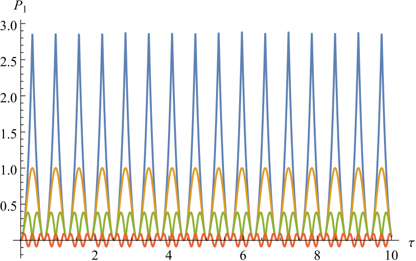
(a)

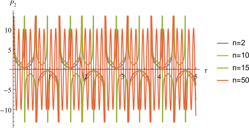
(b)

Figure 1: Perturbations for $m=5$, $\mathcal{E}=0.03$

Now let us discuss perturbation equation for $\varphi(\tau,\sigma)$ without any approximation. Substituting $sn^{2}(m\tau,\frac{\mathcal{E}^{2}}{m^{2}})=s$ in the equation (28), the equation takes the form

$$\frac{\partial^{2}\alpha_{n}}{\partial s^{2}}+\frac{1}{2}\left(\frac{1}{s}+\frac{1}{s-1}+\frac{1}{s-\frac{m^{2}}{\mathcal{E}^{2}}}\right)\frac{\partial\alpha_{n}}{\partial s}+\frac{1}{s(s-1)(s-\frac{m^{2}}{\mathcal{E}^{2}})}\left(\frac{n^{2}+\mathcal{E}^{2}}{4\mathcal{E}^{2}}-\frac{m^{2}}{2\mathcal{E}^{2}s}\right)\alpha_{n}=0.$$ (33)

Since the differential equation have four regular singular points i.e $0,1,\frac{m^{2}}{\mathcal{E}^{2}}~{}\text{and}~{}\infty$, it can be converted into Heun’s equation by proper transformation. Now putting $\alpha_{n}=us$ in equation (33), we have

$$\frac{\partial^{2}u}{\partial s^{2}}+\frac{1}{2}\left(\frac{5}{s}+\frac{1}{s-1}+\frac{1}{s-\frac{m^{2}}{\mathcal{E}^{2}}}\right)\frac{\partial u}{\partial s}+\frac{1}{s(s-1)(s-\frac{m^{2}}{\mathcal{E}^{2}})}\left(\frac{3}{2}s+\frac{n^{2}-4m^{2}}{4\mathcal{E}^{2}}-\frac{3}{4}\right)u=0.$$ (34)

which is exactly the canonical form of Heun’s general equation(see the Appendix) and the solution to this equation can be written in terms of Heun’s function. In general the Heun’s function can be expanded in terms of hypergeometric functions, but we shall not go into details here. So finally the solution of the perturbation equation becomes

$$\alpha_{n}(\tau)=\varepsilon_{0}~{}sn^{2}(m\tau,\frac{\mathcal{E}^{2}}{m^{2}})~{}~{}H\left(\frac{m^{2}}{\mathcal{E}^{2}},\frac{3}{4}-\frac{n^{2}-4m^{2}}{4\mathcal{E}^{2}};\frac{3}{2},1,\frac{5}{2},\frac{1}{2};sn^{2}(m\tau,\frac{\mathcal{E}^{2}}{m^{2}})\right).$$ (35)

As before, we have included $\varepsilon_{0}$ here which is the amplitude of perturbation.

4 Perturbation of pulsating string in $AdS_{3}$

In this section we consider the pulsating string in $AdS_{3}$ background and then we find the equation of motion of the worldsheet perturbation. The relevant metric is given by

$$ds^{2}=-\cosh^{2}\rho dt^{2}+d\rho^{2}+\sinh^{2}\rho d\theta^{2}.$$ (36)

The ansatz for the pulsating string:

$$t=t(\tau),~{}~{}~{}~{}~{}~{}~{}~{}~{}\rho=\rho(\tau),~{}~{}~{}~{}~{}~{}~{}~{}\theta=m\sigma.$$ (37)

The string is pulsating along the radial direction of $AdS$ space whereas it spreads over the $\theta$ direction with winding number $m$. We can find the equation of motion for $\rho$,

$$\ddot{\rho}+\cosh\rho\sinh\rho(\dot{t}^{2}+m^{2})=0.$$ (38)

The conserved $AdS$ energy is given by,

$$\mathcal{E}=-\frac{\partial\mathcal{L}}{\partial\dot{t}}=\dot{t}\cosh^{2}\rho.$$ (39)

Now we can write Virasoro constraint equation in terms of $AdS$ energy

$$\dot{\rho}^{2}-\frac{\mathcal{E}^{2}}{\cosh^{2}\rho}+m^{2}\sinh^{2}\rho=0.$$ (40)

To find the explicit form of $\rho(\tau)$ coordinate, we need to solve the Virasoro constraint equation. So for $\rho(0)=0$, the solution for $\rho$ becomes

$$\sinh\rho=\sqrt{\frac{-R_{+}R_{-}}{R_{+}-R_{-}}}sd\left(m\sqrt{R_{+}-R_{-}}\tau|\frac{R_{+}}{R_{+}-R_{-}}\right),$$ (41)

where

$$R_{\pm}=\frac{-m\pm\sqrt{m^{2}+4\mathcal{E}^{2}}}{2m}.$$ (42)

We can note that the solution is periodic since the value of $\frac{R_{+}}{R_{+}-R_{-}}\textless 1$. The value of $\rho$ starts from zero and it reaches maximum value $\rho_{max}=\sinh^{-1}\sqrt{R_{+}}$ and again contracts to zero and so on. The periodic nature of the solution shows that the string is pulsating in $\rho$ direction. The induced metric is given by,

$$ds^{2}=m^{2}\sinh^{2}\rho[-d\tau^{2}+d\sigma^{2}].$$ (43)

The curvature scalar of the worldsheet metric turns out to be:

$${}^{2}R=-2\frac{(\mathcal{E}^{2}+m^{2}\sinh^{4}\rho)}{m^{2}\sinh^{4}\rho}.$$ (44)

The curvature scalar shows that there is singularity at the center of AdS which corresponds to $\frac{2n}{m\sqrt{R_{+}-R_{-}}}\textbf{K}\left(\frac{R_{+}}{R_{+}-R_{-}}\right)$ value of $\tau$. When the string passes through the center of AdS it becomes pointlike and the world-sheet has a curvature singularity. The tangent vectors are given by

$$\dot{X}^{\mu}=\left(\frac{\mathcal{E}}{\cosh^{2}\rho},~{}~{}~{}~{}\sqrt{\frac{\mathcal{E}^{2}}{\cosh^{2}\rho}-m^{2}\sinh^{2}\rho},~{}~{}~{}0\right),~{}~{}~{}X^{\prime\mu}=(0,~{}~{}0,~{}~{}m).$$ (45)

The normal vector satisfying the orthogonality relation (6) is

$$N^{\mu}=\left(\frac{\sqrt{\mathcal{E}^{2}-m^{2}\sinh^{2}\rho\cosh^{2}\rho}}{m\sinh\rho\cosh^{2}\rho},~{}~{}\frac{\mathcal{E}}{m\sinh\rho\cosh\rho},~{}~{}0\right).$$ (46)

The components of extrinsic curvature tensor are,

$$K_{\tau\tau}=-m\mathcal{E},~{}~{}~{}~{}K_{\tau\sigma}=0,~{}~{}~{}~{}~{}K_{\sigma\tau}=0,~{}~{}~{}~{}~{}K_{\sigma\sigma}=-m\mathcal{E}.$$ (47)

Now using (15), we can write first order perturbation equation as

$$-\ddot{\varphi}(\tau,\sigma)+\varphi^{\prime\prime}(\tau,\sigma)+\left(\frac{2\mathcal{E}^{2}}{\sinh^{2}\rho}-2m^{2}\sinh^{2}\rho\right)\varphi(\tau,\sigma)=0.$$ (48)

Using Fourier expansion method i.e. $\varphi(\tau,\sigma)=\sum_{n}\alpha_{n}(\tau)e^{in\sigma}$ and substituting the value of $\sinh\rho$ from (41), the perturbation equation takes the form

$$\ddot{\alpha}_{n}(\tau)+\left(n^{2}-\frac{2\mathcal{E}^{2}}{a^{2}sd^{2}(b\tau,c)}+2m^{2}a^{2}sd^{2}(b\tau,c)\right)\alpha_{n}(\tau)=0,$$ (49)

where

$$a=\sqrt{\frac{-R_{+}R_{-}}{R_{+}-R_{-}}},~{}~{}b=m\sqrt{R_{+}-R_{-}}~{}~{}\text{and}~{}~{}c=\frac{R_{+}}{R_{+}-R_{-}}.$$

The above equation is a generalized Lamé equation or Heun equation with four regular singularities whose general solution can be written in terms of infinite sum of hypergeometric functions. But here we will not discuss details about it, we will consider the perturbation only for special case i.e. for short string solution.

For short string limit $\varepsilon<<m$, the solution for $\rho$ reduces to

$$\sinh\rho\approx\frac{\mathcal{E}}{m}\sin m\tau.$$ (50)

Taking the above approximation, the perturbation equation for short string limit turns out be

$$\ddot{\alpha}_{n}(\tau)+\left(n^{2}-\frac{2m^{2}}{\sin^{2}m\tau}\right)\alpha_{n}(\tau)=0,$$ (51)

The general solution of the above equation can be written in terms of linear combination of two hypergeometric functions

$$\alpha_{n}=C_{1}\sin^{2}m\tau~{}P_{1}(\tau)+C_{2}\frac{1}{\sin m\tau}~{}P_{2}(\tau)$$ (52)

where

$$P_{1}(\tau)={}_{2}F_{1}\left(1+\frac{n}{2m},1-\frac{n}{2m},\frac{5}{2};sin^{2}m\tau\right)~{}~{}~{}\text{and}~{}~{}~{}P_{2}(\tau)={}_{2}F_{1}\left(\frac{n-m}{2m},\frac{-n-m}{2m},-\frac{1}{2};sin^{2}m\tau\right).$$

Our general solution is the combination two independent solutions for any value of $n$, out of which one is oscillatory and other one is divergent solution. The scalar function $\varphi(\tau,\sigma)$ in the perturbation equation takes the form

$$\varphi(\tau,\sigma)=\varepsilon_{0}\sum_{n}\left[C_{1}\sin^{2}m\tau~{}P_{1}(\tau)+C_{2}\frac{1}{\sin m\tau}~{}P_{2}(\tau)\right]e^{in\sigma}.$$ (53)

As described in $R\times S^{2}$ case, here also the diverging term in the perturbation gives instabilities to the solution. Finally we write the physical perturbation to the coordinates of $AdS_{3}$ by using oscillatory solution of the perturbation equation

$$\delta t = N^{t}\varphi(\tau,\sigma)=\varepsilon_{0}\sum_{n}\sin m\tau\cos m\tau\cos n\sigma~{}~{}{}_{2}F_{1}\left(1+\frac{n}{2m},1-\frac{n}{2m},\frac{5}{2};sin^{2}m\tau\right),$$

$$\delta\rho = N^{\rho}\varphi(\tau,\sigma)=\varepsilon_{0}\sum_{n}\sin m\tau\cos n\sigma~{}~{}{}_{2}F_{1}\left(1+\frac{n}{2m},1-\frac{n}{2m},\frac{5}{2};sin^{2}m\tau\right),$$

$$\delta\theta = N^{\theta}\varphi(\tau,\sigma)=0.$$

5 Pulsating string in $AdS_{3}$ with NS-NS B-field

In this section we include the nonvanishing NS-NS B-field for pulsating string in $AdS_{3}$ background. The relevant metric and NS-NS B-field are given by

$$ds^{2}=-\cosh^{2}\rho dt^{2}+d\rho^{2}+\sinh^{2}\rho d\phi^{2},$$

$$B_{t\phi}=q\sinh^{2}\rho,$$ (54)

where the parameter q takes value from 0 to 1. For 0 and 1 value of q the background is supported by pure RR flux and pure NS-NS flux respectively. Now taking the ansatz, $t=t(\tau),~{}\rho=\rho(\tau),~{}\phi=m\sigma,$ the corresponding action becomes

$$I=\frac{1}{4\pi\alpha\prime}\int d\tau d\sigma[-\cosh^{2}\rho\dot{t}^{2}+\dot{\rho}^{2}-m^{2}\sinh^{2}\rho+2qm\sinh^{2}\rho\dot{t}].$$ (55)

Equations of motion for t and $\rho$ are given by

$$\dot{t}\cosh^{2}\rho-\mathcal{E}-qm\sinh^{2}\rho=0,$$

$$\ddot{\rho}+\sinh\rho\cosh\rho(\dot{t}^{2}+m^{2}-2qm\dot{t})=0,$$ (56)

where $\mathcal{E}$ is the energy of AdS. The Virasoro constraint equation reads,

$$-\cosh^{2}\rho\dot{t}^{2}+\dot{\rho}^{2}+m^{2}\sinh^{2}\rho=0.$$ (57)

From equations (5) and (57), we get the expression for $\rho$

$$\dot{\rho}^{2}=\dfrac{(\mathcal{E}+qm\sinh^{2}\rho)^{2}}{\cosh^{2}\rho}-m^{2}\sinh^{2}\rho$$ (58)

For $\rho(0)=0$ the above equation can be solved in terms Jacobi elliptic function,

$$\sinh\rho=\sqrt{\frac{-R_{+}R_{-}}{R_{+}-R_{-}}}sd\left(m\sqrt{1-q^{2}}\sqrt{R_{+}-R_{-}}\tau|\frac{R_{+}}{R_{+}-R_{-}}\right),$$ (59)

where

$$R_{\pm}=\frac{2q\mathcal{E}-m\pm\sqrt{m^{2}-4mq\mathcal{E}+4\mathcal{E}^{2}}}{2m(1-q^{2})}.$$ (60)

The induced metric and the curvature scalar are given by

$$ds^{2}=m^{2}\sinh^{2}\rho\eta_{ab},~{}~{}~{}~{}^{2}R=-2\frac{(\mathcal{E}^{2}+(1-q^{2})m^{2}\sinh^{4}\rho)}{m^{2}\sinh^{4}\rho}.$$ (61)

The tangent and normal vectors are given by

$$\dot{X}^{\mu} = \left(\frac{\mathcal{E}+qm\sinh^{2}\rho}{\cosh^{2}\rho},~{}~{}\sqrt{\dfrac{(\mathcal{E}+qm\sinh^{2}\rho)^{2}}{\cosh^{2}\rho}-m^{2}\sinh^{2}\rho},~{}~{}0\right),~{}~{}X^{\prime\mu}=(0,~{}~{}0,~{}~{}m),$$

$$N^{\mu} = \left(\dfrac{\sqrt{(\mathcal{E}+qm\sinh^{2}\rho)^{2}-m^{2}\sinh^{2}{\rho}\cosh^{2}\rho}}{m\sinh\rho\cosh^{2}\rho},\quad\dfrac{\mathcal{E}+qm\sinh^{2}\rho}{m\sinh\rho\cosh\rho},\quad 0\right).$$ (62)

The components of extrinsic curvature tensor are given by

$$K_{\tau\tau}=-m(\mathcal{E}-mq\sinh^{2}\rho),K_{\sigma\sigma}=-m(\mathcal{E}+mq\sinh^{2}\rho),K_{\tau\sigma}=m^{2}q\sinh^{2}\rho=-K_{\sigma\tau}.$$

Finally we write down the perturbation equation keeping up to 2nd order in $\mathcal{E}$ and first order in $q$

$$\Box\varphi(\tau,\sigma)+2\dfrac{(\mathcal{E}^{2}-m^{2}\sinh^{4}\rho)}{\sinh^{2}\rho}\varphi(\tau,\sigma)-2qm\mathcal{E}\varphi(\tau,\sigma)=0.$$ (64)

Proceeding in the same way as the previous section and substituting $\varphi(\tau,\sigma)=\sum_{n}\alpha_{n}(\tau)e^{in\sigma}$ and extracting the value of $\sinh\rho$ from (59) , the perturbation equation becomes

$$\ddot{\alpha}_{n}(\tau)+\left((n^{2}+2qm\mathcal{E})-\frac{2\mathcal{E}^{2}}{a^{2}sd^{2}(b\tau,c)}+2m^{2}a^{2}sd^{2}(b\tau,c)\right)\alpha_{n}(\tau)=0,$$ (65)

where

$$a=\sqrt{\frac{-R_{+}R_{-}}{R_{+}-R_{-}}},~{}~{}b=m(1-q^{2})\sqrt{R_{+}-R_{-}}~{}~{}\text{and}~{}~{}c=\frac{R_{+}}{R_{+}-R_{-}}.$$

In short string limit $\mathcal{E}<<m$ and for small value of q

$$a\approx\frac{\mathcal{E}}{m-q\mathcal{E}},~{}~{}~{}b\approx m-q\mathcal{E},~{}~{}~{}c\approx 0.$$

Therefore equation (59) becomes

$$\sinh\rho\approx\frac{\mathcal{E}}{m-q\mathcal{E}}\sin(m-q\mathcal{E})\tau.$$ (66)

Taking the above approximation, the perturbation equation for short string turns out to be

$$\ddot{\alpha}_{n}(\tau)+\left((n^{2}+2qm\mathcal{E})-\frac{2(m-q\mathcal{E})^{2}}{\sin^{2}(m-q\mathcal{E})\tau}\right)\alpha_{n}(\tau)=0,$$ (67)

The general solution of this second order differential equation can be written as the superposition of two linearly independent solutions.

$$\alpha_{n}=C_{1}~{}P_{1}(\tau)+C_{2}~{}P_{2}(\tau)$$ (68)

where

$$P_{1}(\tau)=\varepsilon_{0}\sin^{2}(m-q\mathcal{E})\tau~{}~{}{}_{2}F_{1}\left(1+\frac{\sqrt{n^{2}+2qm\mathcal{E}}}{2(m-q\mathcal{E})},1-\frac{\sqrt{n^{2}+2qm\mathcal{E}}}{2(m-q\mathcal{E})},\frac{5}{2};sin^{2}(m-q\mathcal{E})\tau\right)$$ (69)

and

$$P_{2}(\tau)=\frac{\varepsilon_{0}}{\sin(m-q\mathcal{E})\tau}~{}~{}{}_{2}F_{1}\left(\frac{\sqrt{n^{2}+2qm\mathcal{E}}}{2(m-q\mathcal{E})}-\frac{1}{2},-\frac{\sqrt{n^{2}+2qm\mathcal{E}}}{2(m-q\mathcal{E})}-\frac{1}{2},-\frac{1}{2};sin^{2}(m-q\mathcal{E})\tau\right).$$ (70)

The scalar function $\varphi(\tau,\sigma)$ in the perturbation equation takes the form

$$\varphi(\tau,\sigma)=\varepsilon_{0}\sum_{n}\left(C_{1}P_{1}(\tau)+C_{2}P_{2}(\tau)\right)e^{in\sigma}$$ (71)

Here we can also find as similar to the previous sections that in the solution to the perturbation equation one part is finite and oscillatory while other one is diverging making the solution unstable. Finally the physical perturbations to the background coordinates are given by

$$\delta t = N^{t}\varphi(\tau,\sigma)$$

$$= \varepsilon_{0}\sum_{n}\sin(m-q\varepsilon)\tau~{}\cos n\sigma~{}~{}\sqrt{\left(1-\frac{q\varepsilon}{m}\right)^{2}-\left(1-\frac{2q}{m}\right)\sin^{2}(m-q\varepsilon)}$$

$$\times {}_{2}F_{1}\left(1+\frac{\sqrt{n^{2}+2qm\mathcal{E}}}{2(m-q\mathcal{E})},1-\frac{\sqrt{n^{2}+2qm\mathcal{E}}}{2(m-q\mathcal{E})},\frac{5}{2};sin^{2}(m-q\mathcal{E})\tau\right),$$

$$\delta\rho = N^{\rho}\varphi(\tau,\sigma)$$

$$= \varepsilon_{0}\sum_{n}\sin(m-q\mathcal{E})\tau~{}\cos n\sigma\left[\left(1-\frac{q\varepsilon}{m}\right)-\frac{q\varepsilon}{m\left(1-\frac{q\varepsilon}{m}\right)}\sin^{2}(m-q\mathcal{E})\tau\right]$$

$$\times {}_{2}F_{1}\left(1+\frac{\sqrt{n^{2}+2qm\mathcal{E}}}{2(m-q\mathcal{E})},1-\frac{\sqrt{n^{2}+2qm\mathcal{E}}}{2(m-q\mathcal{E})},\frac{5}{2};sin^{2}(m-q\mathcal{E})\tau\right),$$

$$\delta\theta = N^{\theta}\varphi(\tau,\sigma)=0.$$ (72)

It can be seen that, as expected when $q=0$, these results reduce to the results of the previous section. Some comments regarding the perturbation equations and their solutions are in order. The $B$-field influences the solution through its functional form as well as the parameters present there. Therefore, the perturbation equations are different as the classical field equation is different. It is easy to check that the physical perturbations of the pulsating strings in AdS background with flux is more stable compared to the case when there is no flux.

6 Concluding remarks

In this paper, first we discuss the general formalism for the construction of perturbation equation using Polyakov action and in the presence of NS-NS flux. The geometric covariant quantities like normal fundamental form and extrinsic curvature tensor have been introduced to write the perturbation equations. By using pulsating string ansatz, we obtain the solution of the equations of motion and constraints in different subspaces of $AdS_{3}\times S^{3}$ background. In our analysis, we find the resulting perturbation equations in form of hypergeometric differential equations. The solutions to the perturbation equations have been found to be linear combination of oscillatory and diverging part. We find the physical perturbation by taking only the oscillatory part of the solution.

We wish to mention that the second order fluctuation of pulsating strings in $AdS_{5}\times S^{5}$ was discussed in Beccaria:2010zn by single gap Lamé form. In the present paper, we generalize the results in the presence of NS-NS flux. Further, we write down explicit solutions to the perturbation equations by reducing them to problems in the exactly solvable models. The covariant formalism essentially presents the quadratic action of the string in bosonic sector in terms of scalar quantities and covariants of the geometry and it is an elegant method of studying the perturbations. This work is believed to be helpful in finding the first order correction to the energy which correspond to the anomalous dimension of the gauge theory operators in strong coupling regime. Further extension of perturbation of fermionic part of the Green-schwarz action would be worth attempting. We wish to comeback to this issue in future.

Appendix A Appendix

Elliptic integral and Jacobi elliptic function:

In this appandix we collect some relevant formulas we have used in this paper. The incomplete elliptic integral of first kind is defined as

$$\mathbb{F}(\phi,m)=\int_{0}^{\phi}\frac{d\theta}{\sqrt{1-msin^{2}\theta}},$$ (73)

where the range of modulus m and amplitude $\phi$ are $0\leq m\leq 1$ and $0\leq\phi\leq\frac{\pi}{2}$ respectively. The incomplete elliptic integral of first kind becomes complete elliptic integral when $\phi=\frac{\pi}{2}$,

$$\mathbb{K}(m)=\int_{0}^{\frac{\pi}{2}}\frac{d\theta}{\sqrt{1-msin^{2}\theta}}$$ (74)

Similarly the incomplete and complete integral of second kind are defined as

$$\mathbb{E}(m,\phi)=\int_{0}^{\phi}d\theta\sqrt{1-m\sin^{2}\theta},~{}~{}~{}~{}~{}~{}~{}~{}\mathbb{E}(m)=\int_{0}^{\frac{\pi}{2}}d\theta\sqrt{1-m\sin^{2}\theta}$$ (75)

The Jacobi elliptic functions are defined in terms of Jacobi amplitude,

$$\phi=am(u,m)=\mathbb{F}^{-1}(u,m)$$ (76)

$$sn(u,m)=\sin(am(u,m))=\sin\phi$$

$$cn(u,m)=\cos(am(u,m))=\cos\phi$$

$$dn(u,m)=\sqrt{1-m\sin^{2}\phi}=\sqrt{1-m\sin^{2}(am(u,m)}.$$ (77)

Some of the useful properties and relations of Jacobi elliptic functions are Gradshteyn00

$$sd(u,m)=\frac{sn(u,m)}{dn(u,m)},~{}~{}~{}~{}~{}~{}~{}ds(u,m)=\frac{dn(u,m)}{sn(u,m)},$$ (78)

$$cn^{2}(u,m)+sn^{2}(u,m)=1,$$

$$dn^{2}(u,m)+msn^{2}(u,m)=1.$$ (79)

$$sn(u,m) = \frac{1}{\sqrt{m}}sn(\sqrt{m}u,\frac{1}{m}),~{}~{}cn(u,m)=dn(\sqrt{m}u,\frac{1}{m}),~{}~{}dn(u,m)=cn(\sqrt{m}u,\frac{1}{m}),$$

$$sn^{2}(u) = \frac{1-cn(2u)}{1+dn(2u)},~{}~{}~{}~{}~{}sn(u,m)=\frac{1}{\sqrt{m}sn(u+i\mathbb{K}^{\prime}(m),m)}.$$ (80)

The derivatives of Jacobi elliptic functions are:

$$\frac{d}{du}sn(u,m) = cn(u,m)~{}dn(u,m),$$

$$\frac{d}{du}cn(u,m) = -sn(u,m)~{}dn(u,m),$$

$$\frac{d}{du}dn(u,m) = -msn(u,m)~{}cn(u,m).$$ (81)

Heun’s Equation:

Heun’s equation is a second-order linear ordinary differential equation (ODE) of the form

$$\frac{\partial^{2}u}{\partial s^{2}}+\left(\frac{\gamma}{s}+\frac{\delta}{s-1}+\frac{\epsilon}{s-a}\right)\frac{\partial u}{\partial s}+\frac{\alpha\beta s-q}{s(s-1)(s-a)}u=0$$ (82)

with the condition $\alpha+\beta+1=\gamma+\delta+\epsilon$. Heun’s equation has four regular singular points: $0,1,a$ and $\infty$. The solution to the Heun’s equation can be written in terms of Heun function $H(a,q;\alpha,\beta,\gamma,\delta;s)$.

Lamé Equation:

Lamé equation is a second-order ordinary differential equation comes in the method of separation of variables to the Laplace equation in ellipsoidal coordinates. Lamé equation can be expressed in terms of Jacobi elliptic functions as wang1989special ,

$$\frac{d^{2}\Lambda}{d\alpha^{2}}-\left(n(n+1)k^{2}sn^{2}\alpha+E\right)\Lambda=0.$$ (83)

For different values of n the solutions and the corresponding eigenvalues are given as follows,

$$\text{for}~{}~{}n = 0:\Lambda=1,~{}~{}E=0$$

$$n = 1:\Lambda^{-1}=sn(\alpha),~{}~{}\Lambda^{0}=\sqrt{sn^{2}(\alpha)-1},~{}~{}\Lambda^{1}=\sqrt{sn^{2}(\alpha)-\frac{1}{k^{2}}},$$ (84)

$$~{}~{}~{}~{}E^{-1}=-k^{2}-1,~{}~{}E^{0}=-1,~{}~{}E^{1}=-k^{2}.$$

References

- (1) S. S. Gubser, I. R. Klebanov and A. M. Polyakov, A Semiclassical limit of the gauge / string correspondence, Nucl. Phys. B636 (2002) 99–114, [hep-th/0204051].
- (2) A. A. Tseytlin, Review of AdS/CFT Integrability, Chapter II.1: Classical AdS5xS5 string solutions, Lett. Math. Phys. 99 (2012) 103–125, [1012.3986].
- (3) H. J. de Vega and N. G. Sanchez, A New Approach to String Quantization in Curved Space-Times, Phys. Lett. B197 (1987) 320–326.
- (4) H. J. de Vega and N. G. Sanchez, Quantum Dynamics of Strings in Black Hole Space-times, Nucl. Phys. B309 (1988) 552–576.
- (5) H. J. de Vega and N. G. Sanchez, The Scattering of Strings by a Black Hole, Nucl. Phys. B309 (1988) 577–590.
- (6) J. Garriga and A. Vilenkin, Perturbations on domain walls and strings: A Covariant theory, Phys. Rev. D44 (1991) 1007–1014.
- (7) J. Guven, Covariant perturbations of domain walls in curved space-time, Phys. Rev. D48 (1993) 4604–4608, [gr-qc/9304032].
- (8) A. L. Larsen and V. P. Frolov, Propagation of perturbations along strings, Nucl. Phys. B414 (1994) 129–146, [hep-th/9303001].
- (9) A. L. Larsen and N. G. Sanchez, Strings propagating in the (2+1)-dimensional black hole anti-de Sitter space-time, Phys. Rev. D50 (1994) 7493–7518, [hep-th/9405026].
- (10) A. L. Larsen, Stable and unstable circular strings in inflationary universes, Phys. Rev. D51 (1995) 4330–4336, [hep-th/9403193].
- (11) S. Kar and S. Mahapatra, Planetoid strings: Solutions and perturbations, Class. Quant. Grav. 15 (1998) 1421–1436, [hep-th/9701173].
- (12) N. Drukker, D. J. Gross and A. A. Tseytlin, Green-Schwarz string in AdS(5) x S**5: Semiclassical partition function, JHEP 04 (2000) 021, [hep-th/0001204].
- (13) N. Drukker and V. Forini, Generalized quark-antiquark potential at weak and strong coupling, JHEP 06 (2011) 131, [1105.5144].
- (14) S. Frolov and A. A. Tseytlin, Multispin string solutions in AdS(5) x S**5, Nucl. Phys. B668 (2003) 77–110, [hep-th/0304255].
- (15) S. Frolov and A. A. Tseytlin, Quantizing three spin string solution in AdS(5) x S**5, JHEP 07 (2003) 016, [hep-th/0306130].
- (16) S. A. Frolov, I. Y. Park and A. A. Tseytlin, On one-loop correction to energy of spinning strings in S**5, Phys. Rev. D71 (2005) 026006, [hep-th/0408187].
- (17) H. Fuji and Y. Satoh, Quantum fluctuations of rotating strings in AdS(5) x S**5, Int. J. Mod. Phys. A21 (2006) 3673–3698, [hep-th/0504123].
- (18) A. Khan and A. L. Larsen, Improved stability for pulsating multi-spin string solitons, Int. J. Mod. Phys. A21 (2006) 133–150, [hep-th/0502063].
- (19) S. Frolov and A. A. Tseytlin, Semiclassical quantization of rotating superstring in AdS(5) x S**5, JHEP 06 (2002) 007, [hep-th/0204226].
- (20) M. Beccaria, G. V. Dunne, G. Macorini, A. Tirziu and A. A. Tseytlin, Exact computation of one-loop correction to energy of pulsating strings in , J. Phys. A44 (2011) 015404, [1009.2318].
- (21) V. Forini, V. G. M. Puletti and O. Ohlsson Sax, The generalized cusp in x and more one-loop results from semiclassical strings, J. Phys. A46 (2013) 115402, [1204.3302].
- (22) R. Roiban, A. Tirziu and A. A. Tseytlin, Two-loop world-sheet corrections in AdS(5) x S**5 superstring, JHEP 07 (2007) 056, [0704.3638].
- (23) V. Kiosses and A. Nicolaidis, Second order perturbations of relativistic membranes in curved spacetime, Phys. Rev. D89 (2014) 124016, [1404.4166].
- (24) L. Bianchi, M. S. Bianchi, A. Bres, V. Forini and E. Vescovi, Two-loop cusp anomaly in ABJM at strong coupling, JHEP 10 (2014) 013, [1407.4788].
- (25) B. Hoare, Y. Iwashita and A. A. Tseytlin, Pohlmeyer-reduced form of string theory in AdS(5) x S(5): Semiclassical expansion, J. Phys. A42 (2009) 375204, [0906.3800].
- (26) V. Forini, V. G. M. Puletti, L. Griguolo, D. Seminara and E. Vescovi, Remarks on the geometrical properties of semiclassically quantized strings, J. Phys. A48 (2015) 475401, [1507.01883].
- (27) S. Bhattacharya, S. Kar and K. L. Panigrahi, Perturbations of spiky strings in flat spacetimes, JHEP 01 (2017) 116, [1610.09180].
- (28) B. Hoare and A. A. Tseytlin, On string theory on AdS S T 4 with mixed 3-form flux: tree-level S-matrix, Nucl. Phys. B873 (2013) 682–727, [1303.1037].
- (29) B. Hoare and A. A. Tseytlin, Massive S-matrix of AdS S T 4 superstring theory with mixed 3-form flux, Nucl. Phys. B873 (2013) 395–418, [1304.4099].
- (30) T. Lloyd, O. Ohlsson Sax, A. Sfondrini and B. Stefański, Jr., The complete worldsheet S matrix of superstrings on AdS S T 4 with mixed three-form flux, Nucl. Phys. B891 (2015) 570–612, [1410.0866].
- (31) A. Cagnazzo and K. Zarembo, B-field in AdS(3)/CFT(2) Correspondence and Integrability, JHEP 11 (2012) 133, [1209.4049].
- (32) L. Wulff, Superisometries and integrability of superstrings, JHEP 05 (2014) 115, [1402.3122].
- (33) A. Banerjee, K. L. Panigrahi and P. M. Pradhan, Spiky strings on with NS-NS flux, Phys. Rev. D90 (2014) 106006, [1405.5497].
- (34) R. Hernández and J. M. Nieto, Spinning strings in with NS–NS flux, Nucl. Phys. B888 (2014) 236–247, [1407.7475].
- (35) A. Banerjee, K. L. Panigrahi and M. Samal, A note on oscillating strings in AdS3 × S3 with mixed three-form fluxes, JHEP 11 (2015) 133, [1508.03430].
- (36) R. C. Rashkov and K. S. Viswanathan, Rotating strings with B field, [hep-th/0211197].
- (37) H. Dimov, V. G. Filev, R. C. Rashkov and K. S. Viswanathan, Semiclassical quantization of rotating strings in Pilch-Warner geometry, Phys. Rev. D68 (2003) 066010, [hep-th/0304035].
- (38) A. L. Larsen and M. A. Lomholt, Open string fluctuations in AdS with and without torsion, Phys. Rev. D68 (2003) 066002, [hep-th/0305034].
- (39) J. A. Minahan, Circular semiclassical string solutions on AdS(5) x S(5), Nucl. Phys. B648 (2003) 203–214, [hep-th/0209047].
- (40) S. Bhattacharya, S. Kar and K. L. Panigrahi, “Perturbations of spiky strings in AdS3,” JHEP 1806, 089 (2018) [arXiv:1804.07544 [hep-th]].
- (41) K. S. Viswanathan and R. Parthasarathy, String theory in curved space-time, Phys. Rev. D55 (1997) 3800–3810, [hep-th/9605007].
- (42) I. Gradshteyn and I. Ryzhik, Table of Integrals, Series and Products. Academic Press, New York, sixth ed., 2000.
- (43) Z. Wang and D. Guo, Special Functions. EBL-Schweitzer. World Scientific, 1989.