A theoretical model of the variation of the meridional circulation with the solar cycle

Abstract

Observations of the meridional circulation of the Sun, which plays a key role in the operation of the solar dynamo, indicate that its speed varies with the solar cycle, becoming faster during the solar minima and slower during the solar maxima. To explain this variation of the meridional circulation with the solar cycle, we construct a theoretical model by coupling the equation of the meridional circulation (the $\phi$ component of the vorticity equation within the solar convection zone) with the equations of the flux transport dynamo model. We consider the back reaction due to the Lorentz force of the dynamo-generated magnetic fields and study the perturbations produced in the meridional circulation due to it. This enables us to model the variations of the meridional circulation without developing a full theory of the meridional circulation itself. We obtain results which reproduce the observational data of solar cycle variations of the meridional circulation reasonably well. We get the best results on assuming the turbulent viscosity acting on the velocity field to be comparable to the magnetic diffusivity (i.e. on assuming the magnetic Prandtl number to be close to unity). We have to assume an appropriate bottom boundary condition to ensure that the Lorentz force cannot drive a flow in the subadiabatic layers below the bottom of the tachocline. Our results are sensitive to this bottom boundary condition. We also suggest a hypothesis how the observed inward flow towards the active regions may be produced.

1 Introduction

The meridional circulation is one of the most important large-scale coherent flow patterns within the solar convection zone, the other such important flow pattern being the differential rotation. A strong evidence for the meridional circulation came when low-resolution magnetograms noted that the ‘diffuse’ magnetic field (as it appeared in low resolution) on the solar surface outside active regions formed unipolar bands which shifted poleward, implying a poleward flow at the solar surface (Howard & Labonte, 1981; Wang et al., 1989). A further confirmation for such a flow came from the observed poleward migration of filaments formed over magnetic neutral lines (Makarov et al., 1983; Makarov & Sivaraman, 1989). Efforts for direct measurement of the meridional circulation also began in the 1980s (Labonte & Howard, 1982; Ulrich et al., 1988). The maximum velocity of the meridional circulation at mid-latitudes is of the order of 20 m s^-1.

After the development of helioseismology, there were attempts to determine the nature of the meridional circulation below the solar surface (Giles et al., 1997; Braun & Fan, 1998). The determination of the meridional circulation in the lower half of the convection zone is a particularly challenging problem. Since the meridional circulation is produced by the turbulent stresses in the convection zone, most of the flux transport dynamo models in which the meridional circulation plays a crucial role assume the return flow of the meridional circulation to be at the bottom of the convection zone. In the last few years, several authors presented evidence for a shallower return flow (Hathaway, 2012; Zhao et al., 2013; Schad et al., 2013). However, Rajaguru & Antia (2015) argue that helioseismic data still cannot rule out the possibility of the return flow being confined near the bottom of the convection zone.

Helioseismic measurements indicate a variation of the meridional circulation with the solar cycle. (Chou & Dai, 2001; Beck et al., 2002; Basu & Antia, 2010; Komm et al., 2015). These results are consistent with the surface measurements of Hathaway & Rightmire (2010), who find that the meridional circulation at the surface becomes weaker during the sunspot maximum by an amount of order 5 m s^-1. One plausible explanation for this is the back-reaction of the dynamo-generated magnetic field on the meridional circulation due to the Lorentz force. The aim of this paper is to develop such a model of the variation of the meridional circulation and to show that the results of such a theoretical model are in broad agreement with observational data.

The theory of the meridional circulation is somewhat complicated. The turbulent viscosity in the solar convection zone is expected to be anisotropic, since gravity and rotation introduce two preferred directions at any point within the convection zone. A classic paper by Kippenhahn (1963) showed that an anisotropic viscosity gives rise to meridional circulation along with differential rotation. This work neglected the ‘thermal wind’ that would arise if the surfaces of constant density and constant pressure do not coincide. A more complete model based on a mean field theory of convective turbulence is due to Kitchatinov & Ruediger (1995) and extended further by Kitchatinov & Olemskoy (2011). These authors argue that, in the high Taylor number situation appropriate for the Sun, the meridional circulation should arise from the small imbalance between the thermal wind and the centrifugal force due to the variation of the angular velocity with $z$ (the direction parallel to the rotation axis). See the reviews by Kitchatinov (Kitchatinov, 2011, 2013) for further discussion. If the meridional circulation really comes from a delicate imbalance between two large terms, one would theoretically expect large fluctuations in the meridional circulation. Numerical simulations of convection in a shell presenting the solar convection zone produce meridional circulation which is usually highly variable in space and time (Karak et al., 2014c; Featherstone & Miesch, 2015; Passos et al., 2017). It is still not understood why the observed meridional circulation is much more coherent and stable than what such theoretical considerations would suggest. There are also efforts to understand whether mean field models can produce a meridional circulation more complicated than a single-cell pattern (Bekki & Yokoyama, 2017).

The meridional circulation plays a very critical role in the flux transport dynamo model, which has emerged as a popular theoretical model of the solar cycle. This model started being developed from the 1990s (Wang et al., 1991; Choudhuri et al., 1995; Durney, 1995; Dikpati & Charbonneau, 1999; Nandy & Choudhuri, 2002; Chatterjee et al., 2004) and its current status has been reviewed by several authors (Choudhuri, 2011b, 2014; Charbonneau, 2014; Karak et al., 2014a). The poloidal field in this model is generated near the solar surface from tilted bipolar sunspot pairs by the Babcock–Leighton mechanism and then advected by the meridional circulation to higher latitudes (Dikpati & Choudhuri, 1994, 1995; Choudhuri & Dikpati, 1999). This poleward advection of the poloidal field is an important feature of the flux transport dynamo model and helps in matching various aspects of the observational data. The poloidal field eventually has to be brought to the bottom of the convection zone, where the differential rotation of the Sun acts on it to produce the toroidal field. If the turbulent diffusivity of the convection zone is assumed low, then the meridional circulation is responsible for transporting the poloidal field to the bottom of the convection zone. On the other hand, if the diffusivity is high, then diffusivity can play the dominant role in the transportation of the poloidal field across the convection zone (Jiang et al., 2007; Yeates et al., 2008). We shall discuss this point in more detail later in the paper. Most of the authors working on the flux transport dynamo assumed a one-cell meridional circulation with an equatorward flow at the bottom of the convection zone. This equatorward meridional circulation plays a crucial role in the equatorward transport of the toroidal field generated at the bottom of the convection zone, leading to solar-like butterfly diagrams. In the absence of the meridional circulation, one finds a poleward dynamo wave (Choudhuri et al., 1995). When several authors claimed to find evidence for a shallower meridional circulation, there was a concern about the validity of the flux transport dynamo model. Hazra et al. (2014) showed that, even if the meridional circulation has a much more complicated multi-cell structure, still we can retain most of the attractive features of the flux transport dynamo as long as there is a layer of equatorward flow at the bottom of the convection zone. In the present work, we assume a one-cell meridional circulation.

Most of the papers on the flux transport dynamo are of kinematic nature, in which the only back-reaction of the magnetic field which is often included is the so-called “$\alpha$-quenching”, i.e. the quenching of the generation mechanism of the poloidal field. Usually kinematic models do not include the back-reaction of the magnetic field on the large-scale flows. We certainly expect the Lorentz force of the dynamo-generated magnetic field to react back on the large-scale flows. From observations, we are aware of two kinds of back-reactions on the large-scale flows: solar cycle variations of the differential rotation known as torsional oscillations and solar cycle variations of the meridional circulation (Choudhuri, 2011a). There have been several calculations showing how torsional oscillations are produced by the back-reaction of the dynamo-generated magnetic field (Durney, 2000; Covas et al., 2000; Bushby, 2006; Chakraborty et al., 2009). Rempel (2006) presented a full mean-field model of both the dynamo and the large-scale flows. This model produced both torsional oscillations and the solar cycle variation of the meridional circulation. However, apart from Figure 4(b) in the paper showing the time-latitude plot of $v_{\theta}$ near the bottom of the convection zone, this paper does not study the time variation of the meridional circulation in detail. To the best of our knowledge, this is the only mean-field calculation of magnetic back-reaction on the meridional circulation before our work.

The back-reaction on the meridional circulation should mainly come from the tension of the dynamo-generated toroidal magnetic field. Suppose we consider a ring of toroidal field at the bottom of the convection zone. Because of the tension, the ring will try to shrink in size and this can be achieved most easily by a poleward slip (van Ballegooijen & Choudhuri, 1988). It is this tendency of poleward slip that would give rise to the Lorentz force opposing the equatorward meridional circulation. We show in our calculations based on a mean field model that this gives rise to a vorticity opposing the normal vorticity associated with the meridional circulation and, as this vorticity diffuses through the convection zone, there is a reduction in the strength of the meridional circulation everywhere including the surface. In order to circumvent the difficulties in our understanding of the meridional circulation itself, we develop a theory of how the Lorentz force produces a modification of the meridional circulation with the solar cycle. The important difference of our formalism from the formalism of Rempel (2006) is the following. In Rempel’s formalism, one requires a proper formulation of turbulent stresses to calculate the full meridional circulation in which one sees a cycle variation due to the dynamo-generated Lorentz force. On the other hand, in our formalism, we have developed a theory of the modifications of the meridional circulation due to the Lorentz force so that we can study the modifications of the meridional circulation without developing a full theory of the meridional circulation.

The mathematical formulation of the theory is described in the next Section. Then Section 3 presents the results of our simulation. Our conclusions are summarized in Section 4.

2 Mathematical Formulation

Our main aim is to study how the Lorentz force due to the dynamo-generated magnetic field acts on the meridional circulation. We need to solve the dynamo equations along with the equation for the meridional circulation.

We write the magnetic field in the form

$${\bf B}=B_{\phi}(r,\theta,t)\hat{e}_{\phi}+\nabla\times[A(r,\theta,t)\hat{e}_{\phi}]$$ (1)

where $B_{\phi}$ is the toroidal component of magnetic field and A is the magnetic vector potential corresponding to the poloidal component of the field. Then the dynamo equations for the toroidal and the poloidal components are

$$\frac{\partial A}{\partial t}+\frac{1}{s}({\bf v}_{m}.\nabla)(sA)=\eta_{p}\left(\nabla^{2}-\frac{1}{s^{2}}\right)A+S(r,\theta,t),$$ (2)

$$\frac{\partial B_{\phi}}{\partial t}+\frac{1}{r}\left[\frac{\partial}{\partial r}(rv_{r}B_{\phi})+\frac{\partial}{\partial\theta}(v_{\theta}B_{\phi})\right]=\eta_{t}\left(\nabla^{2}-\frac{1}{s^{2}}\right)B_{\phi}$$

$$+s({\bf B}_{p}.{\bf\nabla})\Omega+\frac{1}{r}\frac{d\eta_{t}}{dr}\frac{\partial{(rB_{\phi})}}{\partial{r}},~{}~{}~{}~{}~{}~{}~{}~{}~{}~{}~{}~{}~{}~{}~{}~{}~{}~{}~{}~{}$$ (3)

where $v_{r}$ and $v_{\theta}$ are components of the meridional flow ${\bf v}_{m}$, $\Omega$ is the differential rotation and $s=r\sin\theta$, whereas $S(r,\theta,t)$ is the source function which incorporates the Babcock-Leighton mechanism and magnetic buoyancy as explained in Chatterjee et al. (2004) and Choudhuri & Hazra (2016). We have kept most of the parameters the same as in Chatterjee et al. (2004). In the kinematic approach, both ${\bf v}_{m}=v_{r}{\bf e}_{r}+v_{\theta}{\bf e}_{\theta}$ and $\Omega$ are assumed to be given.

To understand the effect of the Lorentz force on the meridional circulation, we need to consider the Navier-Stokes equation with the Lorentz force term, which is

$$\frac{\partial{\bf v}}{\partial t}+({\bf v}.\nabla){\bf v}=-\frac{1}{\rho}\nabla p+{\bf g}+{\bf F}_{L}+{\bf F}_{\nu}({\bf v})$$ (4)

where ${\bf v}$ is the total plasma velocity, $\bf g$ is the force due to gravity, ${\bf F}_{L}$ is the Lorentz force term and ${\bf F}_{\nu}({\bf v})$ is the turbulent viscosity term corresponding to the velocity field ${\bf v}$. We would have ${\bf F}_{\nu}({\bf v})=\nu\nabla^{2}{\bf v}$ if the turbulent viscosity $\nu$ is assumed constant in space, but ${\bf F}_{\nu}({\bf v})$ can be more complicated for spatially varying $\nu$. For simplicity we have considered turbulent viscosity as a scalar quantity but, in reality, it is a tensor and can be a quite complicated quantity: see Kitchatinov & Olemskoy (2011). It may be noted that the tensorial nature of turbulent viscosity is quite crucial in the theory of the unperturbed meridional circulation and it cannot be treated as a scalar in the complete theory. To study torsional oscillations, we have to consider the $\phi$ component of Eq. 4 as done by Chakraborty et al. (2009). To consider variations of the meridional circulation, however, we need to focus our attention on the $r$ and $\theta$ components of Eq. 4. A particularly convenient approach is to take the curl of Eq. 4 (noting that $({\bf v}.\nabla){\bf v}=-{\bf v}\times(\nabla\times{\bf v})+\frac{1}{2}\nabla(v^{2})$) and consider the $\phi$ component of the resulting equation. This gives

$$\frac{\partial\omega_{\phi}}{\partial t}-[\nabla\times\{{\bf v}\times(\nabla\times{\bf v})\}]_{\phi}=\frac{1}{\rho^{2}}[\nabla\rho\times\nabla p]_{\phi}$$ (5)

$$~{}~{}+[\nabla\times{\bf F}_{L}]_{\phi}+[\nabla\times{\bf F}_{\nu}({\bf v}_{m})]_{\phi}.$$

where $\omega=\nabla\times{\bf v}$ is the vorticity, of which the $\phi$ component comes from the meridional circulation ${\bf v}_{m}$ only. Writing ${\bf v}={\bf v}_{m}+r\sin\theta\Omega\hat{e}_{\phi}$, a few steps of straightforward algebra give

$$[\nabla\times\{{\bf v}\times(\nabla\times{\bf v})\}]_{\phi}=-r\sin\theta\nabla.\left({\bf v}_{m}\frac{\omega_{\phi}}{r\sin\theta}\right)+r\sin\theta\frac{\partial\Omega^{2}}{\partial z}$$ (6)

Substituting this in Eq. 5, we have

$$\frac{\partial\omega_{\phi}}{\partial t}+s\nabla.\left({\bf v}_{m}\frac{\omega_{\phi}}{s}\right)=s\frac{\partial\Omega^{2}}{\partial z}+\frac{1}{\rho^{2}}(\nabla\rho\times\nabla p)_{\phi}$$ (7)

$$~{}~{}+[\nabla\times{\bf F}_{L}]_{\phi}+[\nabla\times{\bf F}_{\nu}({\bf v}_{m})]_{\phi}.$$

We now break up the meridional velocity into two parts:

$${\bf v}_{m}={\bf v}_{0}+{\bf v}_{1},$$ (8)

where ${\bf v}_{0}$ is the regular meridional circulation the Sun would have in the absence of magnetic fields and ${\bf v}_{1}$ is its modification due to the Lorentz force of the dynamo-generated magnetic field. The azimuthal vorticity $\omega_{\phi}$ can also be broken into two parts corresponding to these two parts of the meridional circulation:

$$\omega_{\phi}=\omega_{0}+\omega_{1}.$$ (9)

It is clear from Eq. 7 that the regular meridional circulation of the Sun in the absence of magnetic fields, which is assumed independent of time in a mean field model, should be given by

$$s\nabla.\left({\bf v}_{0}\frac{\omega_{0}}{s}\right)=s\frac{\partial\Omega^{2}}{\partial z}+\frac{1}{\rho^{2}}(\nabla\rho\times\nabla p)_{\phi}$$ (10)

$$~{}~{}+[\nabla\times{\bf F}_{\nu}({\bf v}_{0})]_{\phi}.$$

This is the basic equation which has to be solved to develop a theory of the regular meridional circulation. The first term in R.H.S is the centrifugal force term, whereas the second term, which can be written as

$$\frac{1}{\rho^{2}}(\nabla\rho\times\nabla p)_{\phi}=-\frac{g}{c_{p}r}\frac{\partial S}{\partial\theta},$$ (11)

is the thermal wind term. This is the term which couples the theory to the thermodynamics of the Sun. So we need to solve the energy transport equation of the Sun in order to develop a theory of the regular meridional circulation, making the problem particularly difficult. In the pioneering study of Kippenhahn (1963), the thermal wind term was neglected. However, we now realize that for the Sun, in which the Taylor number is large, this term has to be important and of the order of the centrifugal term (Kitchatinov & Ruediger, 1995). It may be mentioned that, in the model of the meridional circulation due to Kitchatinov & Ruediger (1995) and Kitchatinov & Olemskoy (2011), the advection term on the L.H.S. of Eq. 10 was neglected. On inclusion of this term, the results were found not to change much (L. Kitchatinov, private communication).

We now subtract Equation 10 from 7, which gives

$$\frac{\partial\omega_{1}}{\partial t}+s\nabla.\left({\bf v}_{0}\frac{\omega_{1}}{s}\right)+s\nabla.\left({\bf v}_{1}\frac{\omega_{0}}{s}\right)$$ (12)

$$~{}=[\nabla\times{\bf F}_{L}]_{\phi}+[\nabla\times{\bf F}_{\nu}({\bf v}_{1})]_{\phi}$$

on neglecting the quadratic term in perturbed quantities ${\bf v}_{1}\omega_{1}$ and assuming that ${\bf F}_{\nu}({\bf v})$ is linear in ${\bf v}$, which is the case if we use the standard expressions of the viscous stress tensor. We have also assumed that the dynamo-generated magnetic fields do not affect the thermodynamics significantly, making the thermal wind term to drop out of Eq. 12. This is what makes the theory of the modification of the meridional circulation decoupled from the thermodynamics of the Sun and simpler to handle than the theory of the unperturbed meridional circulation. We have also not included the centrifugal force term, on the assumption that the temporal variations in $\Omega$ with the solar cycle do not significantly affect our model of the meridional circulation perturbations. The existence of torsional oscillations indicates that this may not be a fully justifiable assumption. In a future work, we plan to include torsional oscillations in the theory along with the meridional circulation perturbations.

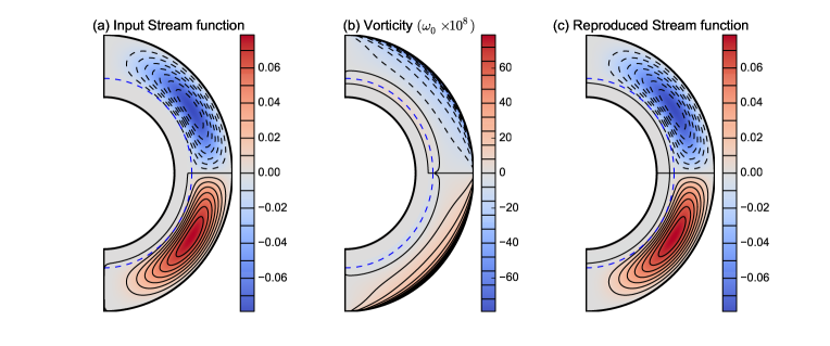
Figure 1: (a) The input stream function for the unperturbed meridional circulation which is used in all of our simulations. The streamlines are indicated by contours—solid contours indicating clockwise flow and dashed contours indicating anti-clockwise flow. (b) The unperturbed vorticity calculated from the stream function shown in (a). Solid and dashed contours indicate positive and negative vorticity. (c) The stream function by inverting the vorticity shown in (b) with the help of Eq. 14. This has to be compared with (a). Blue dashed line represents the tachocline in all plots

In order to study how the meridional circulation evolves with the solar cycle due to the Lorentz force of the dynamo-generated magnetic fields, we need to solve Equation 12 along with Equations 2 and 2. A solution of Eq. 12 first yields the perturbed vorticity $\omega_{1}$ at different steps. We can then compute the perturbed velocity ${\bf v}_{1}$ in the following way. Since $\nabla\cdot\rho{\bf v}_{1}=0$, we can write ${\bf v}_{1}$ in terms of a stream function:

$${\bf v}_{1}=\frac{1}{\rho}\nabla\times[\psi(r,\theta,t)\hat{e}_{\phi}].$$ (13)

Putting this in ${\bf\omega}_{1}=\nabla\times{\bf v}_{1}$, we get

$$\frac{1}{\rho}[\nabla\rho\times\{\nabla\times(\psi\hat{e}_{\phi})\}]_{\phi}+\left(\nabla^{2}-\frac{1}{s^{2}}\right)\psi=-\rho\omega_{1}.$$ (14)

This is similar to Poisson’s equation and we solve it for a given vorticity to get the stream function. After obtaining the stream function, it is very trivial to get the velocity fields. There are various methods to solve this vorticity-stream function equation (Eq. 14), but we choose to solve it using Alternating Direction Implicit (ADI) method. The advantage of this method is that it will take less iterations than the other relaxation methods (e.g, Jacobi iteration method) to achieve the same accuracy level. To check whether this method is giving us the correct results, we take the vorticity of the unperturbed meridional circulation that we use in our dynamo calculations. We invert this vorticity to obtain the velocity field by solving Eq. 14 and then cross check if we have succeeded in reproducing the original input meridional circulation. The stream function corresponding to the input velocity field is shown in Figure 1(a). Here black solid contours surrounding regions of positive stream function (indicated by red) imply clockwise flow and black dashed contours surrounding regions of negative stream function (indicated by blue) imply anti-clockwise flow. We calculate the vorticity (Fig 1(b)) from this given velocity field and solve Eq. 14 to get back the stream function. The stream function obtained in this process is shown in Fig 1(c). As we can see, it is almost indistinguishable from the original given stream function. While solving Eq.  14, we have set the tolerance level to $10^{-5}$, which is found to be sufficient enough to get accurate results. As meridional circulation cannot penetrate much below the tachocline, we have used $v_{r}=0$ at $r=0.65R_{\odot}$ as our bottom boundary condition.

It may be noted that a realistic specification of density $\rho$ is more important for studying the meridional circulation than for the dynamo problem. It is the density stratification which determines how strong the poleward flow at the surface will be compared to the equatorward flow at the bottom of the convection zone. We use a polytropic, hydrostatic, adiabatic stratification for density that matches the standard solar model quite well (Jones et al., 2011):

$$\overline{\rho}=\rho_{i}~{}\left(\frac{\zeta(r)}{\zeta(r_{1})}\right)^{n}$$ (15)

where

$$\zeta(r)=c_{0}+c_{1}\frac{r_{2}-r_{1}}{r}$$ (16)

$$c_{0}=\frac{2\zeta_{0}-\beta-1}{1-\beta}$$ (17)

$$c_{1}=\frac{(1+\beta)(1-\zeta_{0})}{(1-\beta)^{2}}$$ (18)

and

$$\zeta_{0}=\frac{\beta+1}{\beta\exp(N_{\rho}/n)+1}~{}~{}~{}.$$ (19)

Here $\rho_{i}=\rho(r_{1})=0.1788$ g cm^-3, $\beta=r_{1}/r_{2}=0.55$ is the aspect ratio, $n=1.5$ is the polytropic index, and $N_{\rho}=5$ is the number of density scale heights across the computational domain, which extends from $r_{1}=0.55R_{\odot}$ to $r_{2}=R_{\odot}$.

To solve Eq. 12, we need explicit expressions of $[\nabla\times{\bf F}_{L}]_{\phi}$ and $[\nabla\times{\bf F}_{\nu}({\bf v}_{1})]_{\phi}$. If the magnetic field is given by Eq. 1, then we have

$$[\nabla\times{\bf F}_{L}]_{\phi}=\left[\nabla\times\left(\frac{(\nabla\times{\bf B})\times{\bf B}}{4\pi\rho}\right)\right]_{\phi}~{}~{}~{}~{}~{}~{}~{}~{}~{}~{}~{}~{}~{}~{}~{}~{}~{}~{}~{}~{}~{}~{}~{}~{}$$ (20)

$$~{}=\left[\frac{1}{4\pi\rho}\nabla\times\{(\nabla\times{\bf B})\times{\bf B}\}\right]_{\phi}-\left[\{(\nabla\times{\bf B})\times{\bf B}\}\times\nabla\left(\frac{1}{4\pi\rho}\right)\right]_{\phi}$$

It is straightforward to show that

$$\nabla\times\left[\{(\nabla\times{\bf B})\times{\bf B}\}\right]_{\phi}~{}~{}~{}~{}~{}~{}~{}~{}~{}~{}~{}~{}~{}~{}~{}~{}~{}~{}~{}~{}~{}~{}~{}~{}~{}~{}~{}~{}~{}~{}~{}~{}~{}~{}~{}~{}~{}$$ (21)

$$=\left[\frac{1}{r}\frac{\partial}{\partial r}\left(\frac{j_{\phi}}{s}\right)\frac{\partial(sA)}{\partial\theta}-\frac{1}{r}\frac{\partial}{\partial\theta}\left(\frac{j_{\phi}}{s}\right)\frac{\partial(sA)}{\partial r}\right]$$

$$+\left[\frac{1}{r}\frac{\partial}{\partial\theta}\left(\frac{B_{\phi}}{s}\right)\frac{\partial(sB_{\phi})}{\partial r}-\frac{1}{r}\frac{\partial}{\partial r}\left(\frac{B_{\phi}}{s}\right)\frac{\partial(sB_{\phi})}{\partial\theta}\right]$$

where $j_{\phi}=(\nabla\times{\bf B})_{\phi}$ is $\phi$ component of current density, which is associated only with the poloidal field. It is clear from Eq. 21 that the Lorentz forces due to the poloidal field and due to the toroidal field clearly separate out. In typical flux transport dynamo simulations, the toroidal magnetic field turns out to be about two orders of magnitude stronger than the poloidal magnetic field. Since the Lorentz force goes as the square of the magnetic field, the Lorentz force due to the toroidal field should be about four orders of magnitude stronger than that due to the poloidal field. So we include the Lorentz force due to the toroidal field alone in our calculations. We also have to keep in mind that the magnetic field in the convection zone is highly intermittent with a filling factor, say $f$. The Lorentz force is significant only inside the flux tubes and a mean field value of this has to be included in the equations of our mean field theory. This point was discussed by Chakraborty et al. (2009), who showed that, if we use mean field values of the magnetic field in our equations, then the mean field value of the quadratic Lorentz force will involve a division by $f$. Keeping this in mind, the expression of $[\nabla\times{\bf F}_{L}]_{\phi}$ to be used when solving Equation 12 is obtained from Equations 20 and 21:

$$[\nabla\times{\bf F}_{L}]_{\phi}=\frac{1}{4\pi\rho f}\left[\frac{1}{r^{2}}\frac{\partial}{\partial\theta}(B_{\phi}^{2})-\frac{\cot\theta}{r}\frac{\partial}{\partial r}(B_{\phi}^{2})\right]$$ (22)

$$~{}+\frac{1}{4\pi\rho^{2}f}\frac{d\rho}{dr}\frac{B_{\phi}}{r\sin\theta}\frac{\partial(\sin\theta B_{\phi})}{\partial\theta}$$

The expression for $[\nabla\times{\bf F}_{\nu}({\bf v}_{1})]_{\phi}$ happens to be rather complicated (even when the turbulent diffusivity $\nu$ is assumed to be a scalar) and will be discussed in Appendix A. We carry on our calculations assuming a simpler form of the viscosity term:

$$[\nabla\times F_{\nu}({\bf v_{1}})]_{\phi}=\nu\left(\nabla^{2}-\frac{1}{r^{2}\sin^{2}\theta}\right)\omega_{1}.$$ (23)

As we shall show in Appendix A, this simple expression of $[\nabla\times{\bf F}_{\nu}({\bf v}_{1})]_{\phi}$, which is easy to implement in a numerical code, captures the effect of viscosity reasonably well.

To study the variations of the meridional circulation with the solar cycle, we need to solve Equations 2, 2 and 12 simultaneously, with $[\nabla\times{\bf F}_{L}]_{\phi}$ and $[\nabla\times{\bf F}_{\nu}({\bf v}_{1})]_{\phi}$ in Eq. 12 given by Eq. 22 and Eq. 23 respectively. It is the term $[\nabla\times{\bf F}_{L}]_{\phi}$ in Eq. 12 which is the source of the perturbed vorticity $\omega_{1}$ and gives rise the variations of the meridional circulation with the solar cycle. The toroidal field field $B_{\phi}$ obtained at each time step from Eq. 2 is used for calculating $[\nabla\times{\bf F}_{L}]_{\phi}$ as given by Eq. 22.

The numerical procedure for solving Equations 2 and 2 has been discussed in detail by Chatterjee et al. (2004). We solve Eq. 12 also in a similar way. Note that this equation consists of two advection terms in the LHS and one diffusion term along with the source term in the RHS. It is also basically an advection-diffusion equation similar to Eq. 2 and 2. We solve Equation 12 to obtain the axisymmetric perturbed vorticity $\omega_{1}$ in the $r-\theta$ plane of the Sun with $256\times 256$ grid cells in latitudinal and radial directions. As in the case of Equations 2 and 2, we solve Eq. 12 by using Alternating Direction Implicit (ADI) method of differencing, treating the diffusion term through the Crank–Nicholson scheme and the advection term through the Lax–Wendroff scheme (for more detail please see the guide of Surya code which is publicly available upon request. Please send e-mail to arnab@iisc.ac.in). We have used $\omega_{1}=0$ as the boundary condition at the poles $\theta=0$ and $\pi$. The radial boundary conditions are also $\omega_{1}=0$ on the surface $(r=R_{\odot})$ and below the tachocline $(r=0.70R_{\odot})$.

We now make one important point. By solving Eq. 12, we obtain the perturbed vorticity $\omega_{1}$ at each time step. If we need the perturbed velocity ${\bf v}_{1}$ also at a time step, then we further need to solve Eq. 14 over our $256\times 256$ grid points. If this is done at every time step, then the calculation becomes computationally very expensive. It is much easier to run the code if we do not need ${\bf v}_{1}$ at each time step. In a completely self-consistent theory, the meridional flow appearing in the dynamo Equations 2 and 2 should be given by Eq. 8, with ${\bf v}_{1}$ inserted at each time step. As we pointed out, this is computationally very expensive. If ${\bf v}_{1}$ is assumed small compared to ${\bf v}_{0}$, then the dynamo Equations 2 and 2 can be solved much more easily by using ${\bf v}_{m}={\bf v}_{0}$. Additionally, ${\bf v}_{1}$ appears in the third term on the LHS of Eq. 12. We discuss this term in Appendix B, where we argue that our results should not change qualitatively on not including this term. If we neglect this term along with using ${\bf v}_{m}={\bf v}_{0}$ in the dynamo equations 2 and 2, then we do not require ${\bf v}_{1}$ at each time step. The calculations in the present paper are done by following this approach, which is computationally much less intensive. This has enabled us to explore the parameter space of the problem more easily and understand the basic physics issues. We are now involved in the much more computationally intensive calculations in which ${\bf v}_{1}$ is calculated at regular time intervals and the dynamo equations 2 and 2 are solved by including ${\bf v}_{1}$ in the meridional flow. The results of these calculations will be presented in a future paper.

Finally, before presenting our results, we want to point out a puzzle which we are so far unable to resolve. Our calculations suggest that the variations of the meridional circulation should be about two orders of magnitude larger than what they actually are! Since a larger $f$ would reduce the Lorentz force given by Eq. 22, we can make the variations of the meridional circulation to have the right magnitude only if we take the filling factor $f$ larger than unity, which is clearly unphysical. We show that this problem becomes apparent even in a crude order-of-magnitude estimate. We expect $\omega_{1}$ to be of order $V/L$, where $V$ is the perturbed velocity amplitude and $L$ is the length scale. Then $\partial\omega_{1}/\partial t$ has to be of order $V/LT$. Taking $T$ to be the solar cycle period and $L$ to be the depth of the convection zone, a value $V\approx 5$ m s^-1 gives

$$\left|\frac{\partial\omega_{1}}{\partial t}\right|\approx 10^{-16}\rm{s}^{-2}.$$ (24)

The curl of the Lorentz force is the source of this term and should be of the same amplitude. Now the curl of the Lorentz force is of order $|B_{\phi}^{2}/4\pi f\rho L^{2}|$. In a mean field dynamo model, the magnetic field should be scaled such that the mean polar field comes out to have amplitude of order 10 G. Then the mean toroidal field at the bottom of the toroidal field turns out to be about $10^{3}$ G. On using such a value, the curl of the Lorentz force is of order $10^{-15}/f$ s^-2. This would become equal to $10^{-16}$ s^-2 given in Eq. 24 only if $f$ is of order 10—a completely unphysical result. If we take $f$ less than 1 as expected, then the theoretical value of the perturbed meridional circulation would be much larger than what is observed. One may wonder if the same problem would be there in the theory of torsional oscillations. It turns out that the torsional oscillations have the same amplitude 5 m s^-1 as variations in the meridional circulation. However, torsional oscillations are driven by the component $\approx|B_{r}B_{\phi}/L|$ of the magnetic stress rather than the component $\approx|B_{\phi}^{2}/L|$ relevant for meridional circulation variations. Since $|B_{r}|$ turns out to be about 100 times smaller $|B_{\phi}|$ in mean field dynamo calculations, things come out quite reasonably in the theory of torsional oscillations (Chakraborty et al., 2009). Here is then the puzzle. Since the variations in the meridional circulation are driven by the magnetic stress $\approx|B_{\phi}^{2}/L|$ which is about 100 times larger than the magnetic stress $\approx|B_{r}B_{\phi}/L|$ driving torsional oscillations, one would naively expect the meridional circulation variations to have an amplitude about 100 times larger than the amplitude of torsional oscillations. But why are their observational values found comparable? In the present paper, we do not attempt to provide any solution to this puzzle and merely present this as an issue that requires further study. We point out that, even in non-magnetic situations, some terms in the equations tend to produce a much faster meridional circulation than what is observed (Durney, 1996; Dikpati, 2014). Presumably, such a fast meridional circulation would upset the thermal balance and, as a back reaction, a thermal wind force would arise to ensure that such a large meridional circulation does not take place. It needs to be investigated whether similar considerations would hold in the case of magnetic forcing of the meridional circulation as well.

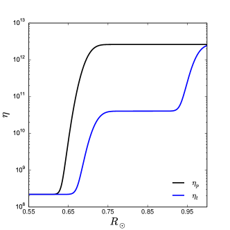
Figure 2: Magnetic diffusivities (cm² s^-1) used in our flux transport model. The black solid line shows the turbulent diffusivity for the poloidal magnetic field, and the blue solid line shows the same for the toroidal magnetic field.

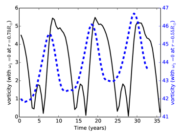
Figure 3: The perturbed vorticity at a point within the convection zone is plotted against time for the two cases with different boundary conditions. The black solid line shows the absolute value of the perturbed vorticity $\omega_{1}$ at 15^∘ latitude and at depth $0.75R_{\odot}$, with the bottom boundary condition $\omega_{1}=0$ at $r=0.7R_{\odot}$. The blue dashed line shows the absolute value of perturbed vorticity $\omega_{1}$ at $15^{\circ}$ latitude and at depth $0.71R_{\odot}$, with the bottom boundary condition $\omega_{1}=0$ at $r=0.55R_{\odot}$. The values of the vorticity which is shown in blue dashed line are given on the right $y$-axis with blue colour.

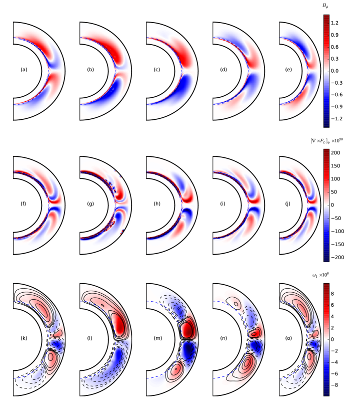
Figure 4: Snapshots in the $r-\theta$ plane of different quantities spanning an entire solar cycle: the toroidal field $B_{\phi}$, the $\phi$ component of the curl of the Lorentz force $[\nabla\times{\bf F}_{L}]_{\phi}$ and the perturbed vorticity $\omega_{1}$ with streamlines are shown in the first row (a)-(e), the second row (f)-(j), and the third row (k)-(o) respectively. The five columns represent time instants during the midst of the rising phase, the solar maximum, the midst of the decay phase and the solar minimum, followed by the midst of the rising phase again. In the third row (k)-(o), the solid black contours represent clockwise flows and the dashed black contours represent anti-clockwise flows. The unit of toroidal fields in the first row is given in terms of $B_{c}$. The Lorentz forces in the second row also are calculated from toroidal fields in the unit of $B_{c}$. The vorticities are given (third row) in s^-1. Here $B_{c}$ is the critical strength of magnetic fields above which the fields are magnetically buoyant and create sunspots (Chatterjee et al., 2004). All the plots are for the magnetic Prandtl number $P_{m}=1$ with the bottom boundary condition $\omega_{1}=0$ at $r=0.7R_{\odot}$.

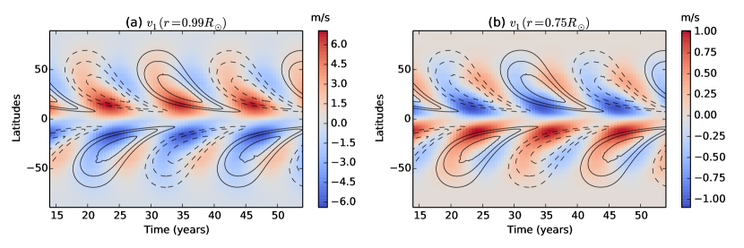
Figure 5: The time–latitude plot of perturbed velocities $v_{\theta}$ (a) near the surface $(r=0.99R_{\odot})$ and (b) at the depth $r=0.75R_{\odot}$. In the northern hemisphere, positive red colour shows perturbed flows towards the equator and the negative blue colour shows flows towards pole. It is opposite in the southern hemisphere. Toroidal fields at the bottom of the convection zone are overplotted in both of the plots by line contours. Black solid contours indicate positive polarity and black dashed contours are for negative polarity. All the plots are for the magnetic Prandtl number $P_{m}=1$ with the bottom boundary condition $\omega_{1}=0$ at $r=0.7R_{\odot}$.

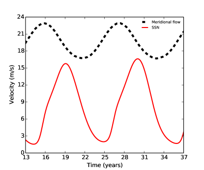
Figure 6: The variation of the total meridional circulation with time is plotted with solar cycle. The yearly averaged solar cycle is plotted in the red solid line, whereas the black dashed line shows the total meridional circulation just below the surface at $25^{\circ}$ latitude.

3 Results

We now present results obtained by solving the dynamo equations  2 and 2 simultaneously with Eq. 12 for perturbed vorticity. The various dynamo parameters—the source function $S(r,\theta,t)$, the differential rotation $\Omega$, the meridional circulation ${\bf v}_{m}$ and the turbulent diffusivities $\eta_{p}$, $\eta_{t}$—are specified as in Chatterjee et al. (2004). As we have pointed out, calculations in this paper are based on using the unperturbed meridional circulation ${\bf v}_{0}$ in the dynamo equations  2 and 2. We also follow Chatterjee et al. (2004) in assuming different diffusivity for the poloidal and the toroidal components of the magnetic field as shown in Fig. 2. The justification for the reduced diffusivity of the toroidal component is that it is much stronger than the poloidal component and the effective turbulent diffusivity experienced by it is expected to be reduced by the magnetic quenching of turbulence. The unquenched value of turbulent diffusivity used for the poloidal field inside the convection zone is what is expected from simple mixing length arguments (Parker (1979), p. 629). A much smaller value of turbulent diffusivity was assumed in some other flux transport dynamo models (Dikpati & Charbonneau, 1999). However, a higher value appears much more realistic on the ground that only with such a higher value it is possible to model many different aspects of observational data: such as the dipolar parity (Chatterjee et al., 2004; Hotta & Yokoyama, 2010), the lack of significant hemispheric asymmetry (Chatterjee & Choudhuri, 2006; Goel & Choudhuri, 2009), the correlation of the cycle strength with the polar field during the previous minimum (Jiang et al., 2007) and the Waldmeier effect (Karak & Choudhuri, 2011). For solving the vorticity Equation 12 we need to specify the turbulent viscosity $\nu$. From simple mixing length arguments, we would expect the turbulent magnetic diffusivity $\eta_{p}$ and the turbulent viscosity $\nu$ to be comparable, i.e, we would expect the magnetic Prandtl number $P_{m}=\nu/\eta_{p}$ to be close to 1. We first present results obtained with $P_{m}=1$ in Section 3.1. How our results get modified on using a lower value of the magnetic Prandtl number $P_{m}$ will be discussed in the Section 3.2.

We know that the toroidal field $B_{\phi}$ changes its sign from one cycle to the next. Since the Lorentz force depends on the square of $B_{\phi}$, as seen in Eq. 22, the Lorentz force should have the same sign in different cycles. As a result, one may think that the perturbed vorticity ${\bf\omega}_{1}$ driven by the Lorentz force will tend to grow. However, results presented in Sections 3.1 and 3.2 are obtained with the boundary condition $\omega_{1}=0$ at $r=0.7R_{\odot}$, which ensures that $\omega_{1}$ cannot grow indefinitely. Asymptotically, we find $\omega_{1}$ to have oscillations as the Lorentz force increases during solar maxima and decreases during solar minima. In Fig. 3 we have shown the time variation of perturbed vorticity (at $15^{\circ}$ latitude and $r=0.75R_{\odot}$) for this case with the black solid line. The calculations presented in Sec. 3.3 were done by taking the boundary condition $\omega_{1}=0$ at $r=0.55R_{\odot}$. In this situation, we found that $\omega_{1}$ has oscillations around a mean which keeps growing with time (see the blue dashed line plot of Fig. 3 which does not saturate even after running the code for several cycles).

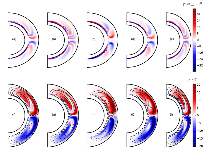
Figure 7: Results obtained with low Prandtl number plotted in the same way as Fig. 4. The top row plotting $[\nabla\times{\bf F}_{L}]_{\phi}$ is the same as the second row of Fig. 4. The bottom row shows the vorticity $\omega_{1}$ with streamlines.

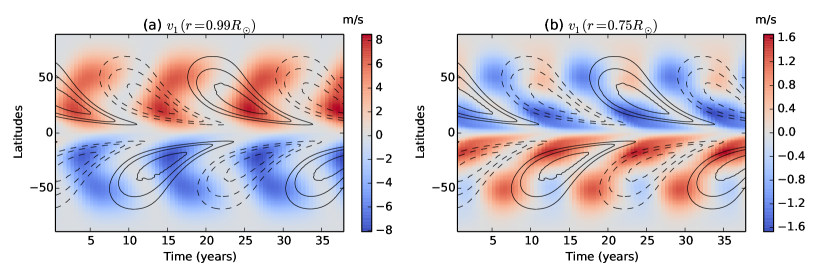
Figure 8: Same as Fig. 5 but with low Prandtl number $P_{m}$.

3.1 Results with $P_{m}=1$

The meridional circulation in a poloidal cut of the Sun’s northern hemisphere is anti-clockwise, implying a negative vorticity $\omega_{0}$. If the meridional circulation is to be weakened by the Lorentz forces at the time of the sunspot maximum, then we need to generate a positive perturbed vorticity $\omega_{1}$ at that time. Fig. 4 explains the basic physics of how this happens. The three rows of this figure plot three quantities in the $r-\theta$ plane: the toroidal field $B_{\phi}$, the $\phi$-component of the curl of the Lorentz force $[\nabla\times{\bf F}_{L}]_{\phi}$ and the perturbed vorticity $\omega_{1}$ along with the associated streamlines. The five vertical columns correspond to five time intervals during a solar cycle. The second column corresponds to a time close to the sunspot maximum, whereas the the fourth column corresponds to the sunspot minimum.

Our discussion of Figure 4 below will refer to the part in the northern hemisphere. Signs will have to be opposite for same quantities in the southern hemisphere. We see in the top row that $B_{\phi}$, produced primarily in the tachocline by the strong differential rotation there, is concentrated in a layer at the bottom of the solar convection zone. Since $-\partial(B_{\phi}^{2})/\partial r$ will be positive at the top of this layer and will be negative at the bottom of this layer, we expect from Eq. 22 that $[\nabla\times{\bf F}_{L}]_{\phi}$ will also respectively have positive and negative values in these regions. This expectation in borne out as seen in the second row of Fig. 4 plotting $[\nabla\times{\bf F}_{L}]_{\phi}$. Where the layer of the toroidal field ends at low latitudes, we have negative $\partial(B_{\phi}^{2})/\partial\theta$ and we see from Eq. 22 that this will lead to negative $[\nabla\times{\bf F}_{L}]_{\phi}$. This is also seen in the second row of Fig. 4. We now note from Eq. 12 that $[\nabla\times{\bf F}_{L}]_{\phi}$ is the main source of the perturbed vorticity $\omega_{1}$. We expect that the positive $[\nabla\times{\bf F}_{L}]_{\phi}$ above the tachocline (i.e. at the top of the layer of concentrated toroidal field) will give rise to positive $\omega_{1}$, implying a clockwise flow opposing the regular meridional circulation. We see in the third row (k)-(o) of Fig. 4 that the distribution of $\omega_{1}$ inside the convection zone follows the distribution of $[\nabla\times{\bf F}_{L}]_{\phi}$ (as shown in the second row (f)-(j)) fairly closely. We see that positive $\omega_{1}$ is particularly dominant within the convection zone near the time of the sunspot maximum (second column). This corresponds to streamlines with clockwise flow, which will oppose the regular meridional circulation at the time of the sunspot maximum and will lead to a decrease in the overall amplitude of the meridional circulation at the solar surface, in accordance with the observational data. It may be interesting to compare Fig. 4 with fig. 3 of Passos et al. (2017), where they present some results on the variation of the meridional circulation with the solar cycle on the basis of a full numerical simulation. Our results obtained from a mean field theory show a spatially smoother perturbed velocity field (perhaps in better agreement with observational data?) than what is found in the full simulation.

We wish to make one important point here. A careful look at the second row of Fig. 4 shows that there is a thin layer of negative $[\nabla\times{\bf F}_{L}]_{\phi}$ at the bottom of the tachocline where $-\partial(B_{\phi}^{2})/\partial r$ is negative. This layer of negative $[\nabla\times{\bf F}_{L}]_{\phi}$ will try to create a negative vorticity driving a counter-clockwise flow below the tachocline. However, we know that it is not easy to drive a flow below the tachocline where the temperature gradient is stable (Gilman & Miesch, 2004). The physics of this is taken into account by using the bottom boundary condition that $\omega_{1}=0$ at $r=0.7R_{\odot}$. As we shall see in Section 3.3, results can change dramatically on changing this boundary condition. Our boundary condition ensures that the negative $[\nabla\times{\bf F}_{L}]_{\phi}$ at the bottom of the tachocline cannot produce negative vorticity there (as seen in the third row of Fig. 4) and cannot drive a flow below the tachocline. We thus see that, while the distribution of $\omega_{1}$ follows the distribution of $[\nabla\times{\bf F}_{L}]_{\phi}$ fairly closely within the convection zone, this is not the case at the bottom of the tachocline.

The strength of the perturbed meridional circulation certainly depends on the strength of $[\nabla\times{\bf F}_{L}]_{\phi}$, which is controlled by the filling factor $f$ as seen in Eq. 22. We have followed the dynamo model of Chatterjee et al. (2004) in which the scale of the magnetic field is set by the critical value $B_{c}$ above which the toroidal field becomes buoyant in the convection zone. As pointed out by Jiang et al. (2007) and followed by Chakraborty et al. (2009), we take $B_{c}=108$ G to ensure that the mean polar field has the right amplitude. With the unit of the magnetic field fixed in this way, we find that $f=53$ gives surface values of the perturbed meridional circulation of the order of 5 m s^-1 comparable to what is seen in the observational data. Such a value of the filling factor $f$, which should be less than 1, is completely unphysical. We anticipated this problem on the basis of the order-of-magnitude estimate presented in Section 2. Chakraborty et al. (2009) needed $f=0.067$ to model torsional oscillations, whereas Choudhuri (2003) estimated that it should be about $f\approx 0.02$. Since $f$ appears in the denominator of the Lorentz force term in Eq. 22, a large value of $f$ means that we have to reduce the Lorentz force in an artificial manner to match theory with observations. We are not sure about the significance of this. All we can say now is that, if we reduce the Lorentz force in this manner, then we find theoretical results to be in good agreement with observational data.

Fig. 5 shows time-latitude plots of the perturbed $v_{\theta}$ just below the surface and in the lower part of the convection zone. Fig. 5(a) can be directly compared with Fig. 11 of Komm et al. (2015). When the perturbed meridional circulation near the surface has an amplitude of about 5 m s^-1 near the surface (comparable to what we find in observational data), its amplitude at the bottom of the convection zone turns out to be about 0.75 m s^-1. This is a significant fraction of the amplitude of the meridional circulation at the bottom of the convection zone, which is of order 2 m s^-1. In other words, the ratio of the amplitude at the bottom of the convection zone to the amplitude at the top of the convection zone for the perturbed meridional circulation ($\approx 0.15$) is somewhat larger than this ratio for the regular meridional circulation($\approx 0.08$). The reason behind this becomes clear on comparing the distribution of $\omega_{0}$, as seen in Fig. 1(b), with the distribution of $\omega_{1}$, as seen in Fig. 4(l), i.e. the second figure in the third row of Fig. 4. This ratio is small when the vorticity is concentrated near the upper part of the convection zone and streamlines in the lower part of the convection zone are fairly spread out. On the other hand, with $\omega_{1}$ distributed throughout the body of the convection zone, this ratio for the perturbed meridional circulation is not so small. The perturbed meridional circulation at the bottom of the convection zone (which is in the poleward direction) will reduce the value of the equatorward meridional circulation there considerably at the time of the sunspot maximum. This will presumably affect the behaviour of the dynamo, in such ways as lengthening its period (since a slower meridional circulation at the bottom of the convection zone during certain phases of the cycle is expected to lengthen the cycle). We are certainly not fully justified in solving the dynamo equations 2–2 by using the regular meridional circulation ${\bf v}_{0}$. However, as we have pointed out in Section 2, in order to include the perturbed meridional circulation in these equations, we need to evaluate the perturbed velocity field at every time step (i.e. not only the perturbed vorticity $\omega_{1}$), which will require considerably more computational efforts. We are currently doing these calculations and will present the results in a forthcoming paper. The aim of the present exploratory paper is to elucidate the basic physics of the problem and not to construct a very complete model. Figure 6 shows the time evolution of the total $v_{\theta}$ at $25^{\circ}$ degree latitude just below the surface along with the sunspot number. We see that the meridional circulation reaches its minimum a little after the sunspot maximum. This figure can be compared with Fig. 4 of Hathaway & Rightmire (2010).

One important aspect of observational data is an inward flow towards the belt of active regions at the time of the sunspot maximum (Cameron & Schüssler, 2010; Komm et al., 2015). We now come to the question whether our model can provide any explanation for this. This inward flow means that the meridional circulation is enhanced in the low latitudes below the sunspot belt and reduced in the higher latitudes. It is thought that the cooling effect of sunspots may drive this inward flow (Spruit, 2003; Gizon & Rempel, 2008). Since this idea is not yet fully established through detailed and rigorous calculations, it is worthwhile to look for alternative explanations. We would like to draw the reader’s attention to the first figure in the bottom row of Fig. 4. In the northern hemisphere, we see positive $\omega_{1}$ (implying clockwise flow) extending over latitudes higher than where sunspots are usually seen. However, we see a region of negative $\omega_{1}$ (implying counter-clockwise flow) at lower latitudes. It is clear that the perturbed meridional circulation is of the nature of an inward flow at the latitudes between the region of positive $\omega_{1}$ on the high-latitude side and the region of negative $\omega_{1}$ on the low-latitude side. We are thus able to obtain an inward flow at the latitudes where sunspots are typically seen, but unfortunately we are getting this at the wrong time—shortly after the sunspot minimum (when there would be no sunspots in that region) rather than at the sunspot maximum. A look at Fig. 5(a) also makes it clear that this inward flow occurs slightly after the sunspot minimum. We are now exploring the question whether, by changing some parameters of the model, it is possible to get this inward flow at the right latitudes at the right phase (around the sunspot maximum) of the solar cycle. If our interpretation is correct, then the inward flow has nothing to do with the actual physical presence of sunspots. While the Lorentz force above the tachocline tends to produce positive vorticity, the low-latitude edge of the toroidal magnetic field belt can be a source of negative vorticity. If the sunspot belt merely happens to be a region having positive $\omega_{1}$ on the high-latitude side and negative $\omega_{1}$ on the low-latitude side, then it will be a region of apparent inward flow. We suggest this as a tentative hypothesis which requires further study. We shall argue in Appendix B that the advection term $s\nabla.({\bf v}_{1}\omega_{0}/s)$ not incorporated in the present study (the third term on the LHS of Eq. 12) may be quite important for modelling the inward flow in active regions.

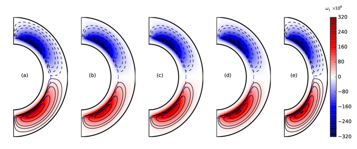
Figure 9: On changing the bottom boundary condition to $\omega_{1}=0$ at $r=0.55R_{\odot}$, the third row of Fig. 4 would get changed to this.

3.2 Results with low Prandtl number $(P_{m}<1)$

In order to study how the nature of the perturbations in the meridional circulation will change on changing the turbulent viscosity $\nu$, we now present results obtained by taking $\nu=\eta_{t}$ (shown by the blue solid line in Fig. 2) rather than $\nu=\eta_{p}$ which was the case for the results presented in Section 3.1. This makes the magnetic Prandtl number defined as $\nu/\eta_{p}$ (note that $\eta_{p}$ rather than $\eta_{t}$ represents the unquenched turbulent diffusivity) much smaller than unity within the body of the convection zone.

We now want to present our results in the meridional plane of the Sun. Since there have been no changes in the dynamo equations  2 and 2, the toroidal field $B_{\phi}$ and the $\phi$-component of the curl of the Lorentz force $[\nabla\times{\bf F}_{L}]_{\phi}$ will be the same as in the first two rows of Fig. 4 if we take the snapshots at the same instants of time. To facilitate easy comparison with the perturbed vorticity $\omega_{1}$ generated, we again plot $[\nabla\times{\bf F}_{L}]_{\phi}$ in the top row of Figure 7. This is the same as the middle row of Fig. 4. Then the bottom row of Figure 7 shows the perturbed vorticity $\omega_{1}$ along with the streamlines of the perturbed velocity. This bottom row should be compared to the bottom row of Fig. 4. When $\nu$ is higher (the case of Fig. 4), the perturbed vorticity $\omega_{1}$ spreads more evenly within the convection zone. On the other hand, when $\nu$ is lower (the case of Figure 7), the perturbed vorticity $\omega_{1}$ tends to be frozen where it is created by $[\nabla\times{\bf F}_{L}]_{\phi}$. As a result, $\omega_{1}$ follows $[\nabla\times{\bf F}_{L}]_{\phi}$ more closely in Figure 7 rather than in Fig. 4. We thus see a more complicated distribution of $\omega_{1}$ in Figure 7 implying a more complicated velocity field.

To make the perturbed meridional circulation near the surface comparable to what we find in the observational data, we need to choose $f=5.3\times 10^{2}$ in this case of low $P_{m}$. This is even more unphysical than what we needed for the case $P_{m}=1$ ($f=53$) with all the other dynamo parameters same. Basically, on reducing viscosity, vorticity tends to get piled up and we need to reduce the strength of the Lorentz force further to match observations. The perturbed velocities near the surface and near the bottom of the convection zone are shown in Fig. 8(a) and 8(b) respectively. The requirement that the perturbed velocity at the surface compares with observational data forces the perturbed velocity at the bottom of the convection zone as seen in Fig. 8(b) of order 1.5 m s^-1, which makes it almost comparable to the unperturbed velocity (though they are in opposite directions). This shows that solving the dynamo equations  2 and 2 with the unperturbed meridional circulation ${\bf v}_{0}$ is more unjustified in this case than in the case of $P_{m}=1$.

We do not know how large the perturbations to the meridional circulation at the bottom of the convection zone actually are. If they were comparable to the unperturbed meridional circulation, then probably we would see some effects on the dynamo. Since this problem has not been studied before, we do not know what those effects may be like. As, on theoretical grounds also we expect $P_{m}$ to be of order unity, we believe that the model with $P_{m}=1$ presented in Section 3.1 is probably a more realistic depiction of what is happening inside the Sun rather than the model with low $P_{m}$.

3.3 Dependence of the results on lower radial boundary condition

While discussing Fig. 4, we have pointed out that the Lorentz force at the bottom of the tachocline would have a tendency of producing a perturbed vorticity with the same sign as the unperturbed vorticity. This will tend to drive a counter-clockwise flow (in the northern hemisphere) below the tachocline. Since on physical grounds we do not expect such a flow to be driven in a region of stable temperature gradient, we have used the boundary condition $\omega_{1}=0$ at $r=0.70R_{\odot}$ in Sections 3.1 and 3.2 to suppress this flow. We found that our results are quite sensitive to this bottom boundary condition. We now discuss what we get on changing the boundary condition to $\omega_{1}=0$ at $r=0.55R_{\odot}$.

Again the solutions of the dynamo equations  2 and 2 remain the same as in Section 3.1 and 3.2. We present the solutions of the perturbed vorticity at the same time instants as the time instants in Figure 4. Only the third row of this figure will be replaced by what is shown in Figure 9. When we had taken the boundary condition $\omega_{1}=0$ at $r=0.70R_{\odot}$ earlier, $\omega_{1}$ was restrained from growing indefinitely. Now, on pushing the boundary well below the bottom of the convection zone, we found that $\omega_{1}$ kept growing for many cycles for which we ran the code (see Fig. 3). This is the reason why the values of $\omega_{1}$ given in the colour scale in Figure 9 are rather large. We would expect the growing perturbed vorticity to have the opposite sign of the original unperturbed vorticity. But this is not the case now. The growing perturbed vorticity has the same sign as the original unperturbed vorticity. This means that the Lorentz force strengthens the original meridional circulation rather than opposing it! Presumably this is because the effect of the Lorentz force at the bottom of the tachocline (which tries to produce a perturbed vorticity of the same sign as the original vorticity) overwhelms the effect of the Lorentz force at the top of the tachocline which opposes the unperturbed meridional circulation. These results show that the bottom boundary condition is quite crucial. If we allow the Lorentz force to create a perturbed vorticity below the bottom of the tachocline, we may get totally unphysical results.

4 Conclusion

The meridional circulation of the Sun plays a crucial role in the flux transport dynamo model, the currently favoured theoretical model for the solar cycle. Presumably an equatorward flow at the bottom of the convection zone is responsible for the equatorward migration of the sunspot belts (Choudhuri et al., 1995; Hazra et al., 2014). The poleward flow at the surface builds up the polar field of the Sun by bringing together the poloidal field generated by the Babcock–Leighton mechanism from the decay of active regions (Hazra et al., 2017). We now have growing evidence that similar flux transport dynamos operate in other solar-like stars as well (Choudhuri, 2017). Our lack of understanding of the meridional circulation in such stars is the major stumbling block for building theoretical models of stellar dynamos (Karak et al., 2014b; Choudhuri, 2017). The mathematical theory of the meridional circulation involves a centrifugal term and a thermal wind term. The centrifugal term couples the theory of the meridional circulation to the theory of differential rotation and the thermal wind term couples the theory to the thermodynamics of the star—making it a very complex subject.

We now have evidence that the meridional circulation of the Sun varies with the solar cycle, becoming weaker around the sunspot maximum (Chou & Dai, 2001; Beck et al., 2002; Hathaway & Rightmire, 2010; Komm et al., 2015). We believe that this is caused by the back-reaction of the Lorentz force of the dynamo-generated magnetic field. We show that the theory of the perturbations to the meridional circulation caused by the Lorentz force can be decoupled from the theory of the unperturbed meridional circulation itself. Especially, this theory becomes decoupled from any thermodynamic considerations if we assume that the magnetic fields do not affect the thermodynamics of the Sun. This makes the theory of the perturbations to the meridional circulation much simpler than the theory of the meridional circulation itself. Even without having a theory of the unperturbed meridional circulation, we are able to develop a theory of how the meridional circulation gets affected by the Lorentz force of the dynamo-generated magnetic fields.

The most convenient way of developing a theory of the meridional circulation is by considering the equation for the $\phi$-component of vorticity $\omega_{\phi}$. We solve the equation for the perturbed vorticity along with the standard axisymmetric mean field equations of the flux transport dynamo. For the unperturbed meridional circulation, $\omega_{\phi}$ is negative in the northern hemisphere of the Sun. If the Lorentz force can produce some positive vorticity there, then we expect the meridional circulation to become weaker during the sunspot maxima. Our calculations show that positive vorticity is indeed produced near the top of the tachocline. Our theoretical results are able to explain many aspects of observational data presented by Hathaway & Rightmire (2010) and Komm et al. (2015) We get best results when the turbulent viscosity $\nu$ is taken to be comparable to the turbulent diffusivity $\eta_{p}$ of the magnetic field, i.e. when the magnetic Prandtl number $P_{m}$ is close to unity. Our results are sensitive to the boundary condition at the bottom of the convection zone. At the bottom of the tachocline, the Lorentz force tends to produce vorticity with the same sign as the unperturbed vorticity and this has to be suppressed with a suitable boundary condition to incorporate the important physics that it is very difficult to drive flows in the stable subadiabatic layers below the tachocline.

One intriguing observation is that of an inward flow towards active regions during the sunspot maxima (Cameron & Schüssler, 2010; Komm et al., 2015). While we have not been able to construct a satisfactory model of this inward flow, we suggest a possibility how this flow may be produced. We would have such a flow if the northern hemisphere has a positive perturbed vorticity at latitudes above the mid-latitudes and a negative perturbed vorticity at lower latitudes. We propose a scenario how this can happen. The Lorentz force at the top of the tachocline tends to produce positive vorticity, whereas the Lorentz force at the edge of the toroidal field belt at low latitudes tends to produce negative vorticity. In our model, we found an inward flow towards typical sunspot latitudes at a wrong phase of the solar cycle. It remains to be seen whether the phase can be corrected by changing the parameters of the problem.

One puzzle we encounter is that we have to reduce the strength of the Lorentz force artificially by about two orders of magnitude to make theory fit with observations. We point out that a similar problem arises in the non-magnetic theory as well. While we do not have a proper explanation for this, we make one comment. While the overall strength of the Lorentz force varies with the solar cycle, it does not change sign between cycles. As a result, the Lorentz force would always tend to drive a very strong clockwise flow in the northern hemisphere (anti-clockwise in the south), if it is not reduced sufficiently. Now, in the theory of the unperturbed meridional circulation, we know that we need some force trying to drive such a flow—to make the surfaces of constant angular velocity depart from cylinders and to balance the centrifugal term. Normally, the thermal wind caused by anisotropic heat transport in the Sun is believed to do this (Kitchatinov & Ruediger, 1995; Kitchatinov & Olemskoy, 2011). Is it possible that the expected large Lorentz force also plays an important in the force balance? To address this question, one has to carry on a much more complicated analysis than what we have attempted in this paper, without separating the equations of unperturbed and perturbed meridional circulation. While we do not attempt such an analysis, our analysis brings out many basic physics issues rather clearly and raises intriguing questions like this.

The equation of the perturbed meridional circulation gives us the perturbed vorticity at different times. In order to get the perturbed velocity from the perturbed vorticity, we need to solve a Poisson-type equation. If we want to do this at every time step, then running the code becomes computationally very expensive. On the hand, if we are satisfied only with the perturbed vorticity at all steps and do not require the perturbed velocity, then we need much less computer time. This is what we have done in this paper in which our aim was to carry out a parameter space study to understand the basic physics. However, we have to pay a price for not calculating the perturbed velocity at all time steps. We keep solving the dynamo equations by using the unperturbed velocity of the meridional circulation. This is certainly a questionable approximation. If we want to make the perturbed velocity at the surface comparable to what is found in observational data ($\approx$ 5 m s^-1), then the perturbed velocity at the bottom of the convection zone turns out to be $\approx$ 0.75 m s^-1. This is certainly smaller than the unperturbed velocity there ($\approx$ 2 m s^-1), but is not completely negligible. While we feel reassured that the perturbed velocity at the bottom of the convection zone is smaller than the unperturbed velocity and probably will not necessitate a major revision of the flux transport dynamo, the effect of this perturbed velocity on the dynamo needs to be investigated. We are now in the process of including this perturbed velocity in the dynamo equations. This will need finding the perturbed velocity from the perturbed vorticity at different time intervals—pushing up the computational requirements significantly. Once we do that, we shall be able to include another advection term involving ${\bf v}_{1}$ in the computations which had been left out in this paper because of computational difficulties. This term may be important for modelling the inward flow towards active regions.

Not including the back-reactions on the meridional circulation in the dynamo equations is not a limitation of this paper alone, but a limitation of nearly all hitherto published papers on the flux transport dynamo based on 2D kinematic mean field formulation. To the best of our knowledge, only Karak & Choudhuri (2012) studied this problem by modelling the back-reaction on the meridional circulation due to the Lorentz force through a simple parameterization (though see Passos et al. (2012) who have included back-reaction in a simple low-order dynamo model). Although such a back-reaction on the meridional circulation can have dramatic effects on the dynamo if the magnetic diffusivity is low, Karak & Choudhuri (2012) found that the effect is not much on a high-diffusivity dynamo (like what we present in this paper). However, it is now important to go beyond such simple parameterization and include the properly computed perturbed velocity in the dynamo equations and study its effects. We hope that we shall be able to present our results in a forthcoming paper in the near future.

Appendix A Calculation of the Viscosity Term

The calculation of the viscous term becomes immensely complicated if $\nabla.{{\bf v}}$ is not set equal to zero. Although we are dealing with a situation in which we rather have $\nabla.(\rho{{\bf v}})=0$, the meridional circulation velocities are everywhere highly subsonic and the role of compressibility in viscous dissipation is expected to be negligible. So we shall assume $\nabla.{{\bf v}}=0$ to make the calculations manageable. For a velocity field

$${\bf v}=v_{r}(r,\theta,t){\bf e}_{r}+v_{\theta}(r,\theta,t){\bf e}_{\theta}$$

the non-zero components of the viscous stress tensor are

$$\sigma_{rr}=2\nu\frac{\partial v_{r}}{\partial r},\sigma_{\theta\theta}=2\nu\left(\frac{1}{r}\frac{\partial v_{\theta}}{\partial\theta}+\frac{v_{r}}{r}\right),~{}~{}~{}~{}~{}~{}~{}~{}~{}~{}~{}~{}~{}~{}~{}~{}~{}~{}~{}~{}~{}~{}$$

$$\sigma_{\phi\phi}=2\nu\left(\frac{v_{r}}{r}+\frac{v_{\theta}\cot\theta}{r}\right),\sigma_{r\theta}=\nu\left(\frac{1}{r}\frac{\partial v_{r}}{\partial\theta}+\frac{\partial v_{\theta}}{\partial r}-\frac{v_{\theta}}{r}\right)$$ (25)

The $r$ and $\theta$ components of the viscosity term in Navier–Stokes equation are given by

$$F_{\nu,r}=\frac{1}{r^{2}}\frac{\partial}{\partial r}(r^{2}\sigma_{rr})+\frac{1}{r\sin\theta}\frac{\partial}{\partial\theta}(\sin\theta\sigma_{r\theta})-\frac{\sigma_{\theta\theta}+\sigma_{\phi\phi}}{r},$$ (26)

$$F_{\nu,\theta}=\frac{1}{r^{2}}\frac{\partial}{\partial r}(r^{2}\sigma_{r\theta})+\frac{1}{r\sin\theta}\frac{\partial}{\partial\theta}(\sin\theta\sigma_{\theta\theta})+\frac{\sigma_{r\theta}}{r}-\frac{\sigma_{\phi\phi}\cot\theta}{r},$$ (27)

We now substitute from Eq. 25 in Equations 26 and 27. On making use of $\nabla.{{\bf v}}=0$, we get after a few steps of algebra

$$F_{\nu,r}=\nu\left[\nabla^{2}v_{r}-\frac{2}{r^{2}}\frac{\partial v_{\theta}}{\partial\theta}-\frac{2v_{r}}{r^{2}}-\frac{2\cot\theta v_{\theta}}{r^{2}}\right]+2\frac{d\nu}{dr}\frac{\partial v_{r}}{\partial r},$$ (28)

$$F_{\nu,\theta}=\nu\left[\nabla^{2}v_{\theta}+\frac{2}{r^{2}}\frac{\partial v_{r}}{\partial\theta}-\frac{v_{\theta}}{r^{2}\sin^{2}\theta}\right]+\frac{d\nu}{dr}\left[\frac{1}{r}\frac{\partial v_{r}}{\partial\theta}+\frac{\partial v_{\theta}}{\partial r}-\frac{v_{\theta}}{r}\right].$$ (29)

To solve Equation 12, we need $[\nabla\times{\bf F}_{\nu}]_{\phi}$, which is given by

$$[\nabla\times{\bf F}_{\nu}]_{\phi}=\frac{1}{r}\left[\frac{\partial}{\partial r}(rF_{\nu,\theta})-\frac{\partial F_{\nu,r}}{\partial\theta}\right].$$ (30)

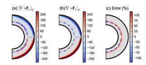
Figure 10: $[\nabla\times{\bf F}_{\nu}]_{\phi}$ calculated using full expression (Eq. 30) and using approximated expression (Eq. 23) are shown in (a) and (b) respectively. The difference between the values of case (a) and (b) are shown in percentage in (c).

On substituting Equations 28 and 29 into Eq. 30, we get a rather complicated analytical expression for the viscosity term. It is extremely challenging to incorporate this complicated expression in the time evolution code to solve Eq. 12—especially if we want to handle the diffusion terms through Crank-Nicholson scheme which is partly implicit, to avoid very small time steps. Since there are many uncertainties in this problem—including the uncertainty in the value of turbulent viscosity $\nu$—we felt that it is not worthwhile to make an enormous effort to incorporate a completely accurate expression of the viscous term in our code to solve Eq. 12. In order to capture the effect of viscosity in the problem, we have used the simpler approximate expression given in Eq. 23. The question is whether we make a very large error in doing this simplification. To address this question, we take the unperturbed meridional circulation shown in Fig. 1(a) and calculate $[\nabla\times{\bf F}_{\nu}]_{\phi}$ for this velocity field both by the approximate expression in Eq. 23 and the full expression in Eq. 30. To calculate the value of $[\nabla\times{\bf F}_{\nu}]_{\phi}$ at different grid points by the full expression in Eq. 30, we first calculate $F_{\nu,r}$ and $F_{\nu,\theta}$ at different grid points by using Equations 28 and 29. Then we use these numerical values of $F_{\nu,r}$ and $F_{\nu,\theta}$ to calculate $[\nabla\times{\bf F}_{\nu}]_{\phi}$ by using a simple difference scheme to handle Eq. 30. The values obtained for $[\nabla\times{\bf F}_{\nu}]_{\phi}$ by using the full expression (Eq. 30) and the approximate expression (Eq. 23) are shown in Figure 10(a) and Figure 10(b) respectively. We see that both the expressions give fairly close values within the main body of the convection zone. Only at the bottom of the convection zone where radial derivatives of $\nu$ included in the full expression are important, the two expressions give somewhat different values—though the values are of the same order of magnitude (see Fig 10(c)). In Figure 10(c), we have shown percentage differences of $[\nabla\times{\bf F}_{\nu}]_{\phi}$ values calculated in two cases (Figures 10(a) and (b)) in our integration region above $r>0.7R_{\odot}$. Note that things change much more at the bottom of the convection zone on changing the bottom boundary condition slightly. We thus conclude that, by using the approximate expression in Eq. 23 for $[\nabla\times{\bf F}_{\nu}]_{\phi}$, we do not make a large error and get everything within the correct order of magnitude.

Appendix B Importance of various advective terms

In the calculations presented in this paper, we have neglected the term $s\nabla.\left({\bf v}_{1}\frac{\omega_{0}}{s}\right)$ while solving Eq. 12, because its evaluation requires the perturbed velocity ${\bf v}_{1}$ in every time step which is computationally very expensive to obtain. Now we calculate the two advective terms in Eq. 12 separately using simple finite difference scheme at a particular time step near a solar maximum to see their relative importance with respect to the Lorentz force term $[\nabla\times{\bf F}_{L}]_{\phi}$. The values of the two advection terms involving unperturbed velocity $s\nabla.\left({\bf v}_{0}\frac{\omega_{1}}{s}\right)$ and involving perturbed velocity $s\nabla.\left({\bf v}_{1}\frac{\omega_{0}}{s}\right)$ in the $r-\theta$ plane are shown in Fig. 11(a) and 11(b) respectively. The $\phi$ component of the curl of the Lorentz force $[\nabla\times{\bf F}_{L}]_{\phi}$ is shown in Fig. 11(c). The colour table for curl of the Lorentz force is clipped to 240 to show its value in the convection zone (where it has much smaller values compared to the tachocline) but its maximum value is about 3000. Thus, in comparison to the curl of the Lorentz force, the other terms are small but not negligible. The advective term $s\nabla.\left({\bf v}_{0}\frac{\omega_{1}}{s}\right)$ which we already included is important within the convection zone, but the other term with perturbed velocity $s\nabla.\left({\bf v}_{1}\frac{\omega_{0}}{s}\right)$ which we plan to include in our future paper is important near the surface at low latitudes. The dynamics of vorticity presented in the Section 3.1 clearly reflect the fact that the time evolution of vorticity is mostly determined by the Lorentz force term $[\nabla\times{\bf F}_{L}]_{\phi}$ (see Fig. 4((k)-(o))) even when the advective term $s\nabla.\left({\bf v}_{0}\frac{\omega_{1}}{s}\right)$ is included. However, since the $s\nabla.\left({\bf v}_{1}\frac{\omega_{0}}{s}\right)$ term becomes appreciable in the regions where we have inward flow towards active regions during the sunspot maximum, this term may have some importance in modelling this inward flow. We plan to investigate this further in future.

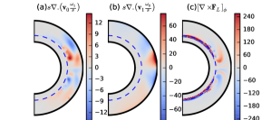
Figure 11: The advective terms in LHS of Eq. 12 are shown in (a) and (b), where $s=r\sin\theta$. The $\phi$ component of the curl of the Lorentz force is shown in (c). All terms are calculated at a particular time step near a solar maximum.

References

- Basu & Antia (2010) Basu S., Antia H. M., 2010, ApJ, 717, 488
- Beck et al. (2002) Beck J. G., Gizon L., Duvall Jr. T. L., 2002, ApJ, 575, L47
- Bekki & Yokoyama (2017) Bekki Y., Yokoyama T., 2017, ApJ, 835, 9
- Braun & Fan (1998) Braun D. C., Fan Y., 1998, ApJ, 508, L105
- Bushby (2006) Bushby P. J., 2006, MNRAS, 371, 772
- Cameron & Schüssler (2010) Cameron R. H., Schüssler M., 2010, ApJ, 720, 1030
- Chakraborty et al. (2009) Chakraborty S., Choudhuri A. R., Chatterjee P., 2009, Physical Review Letters, 102, 041102
- Charbonneau (2014) Charbonneau P., 2014, ARA&A, 52, 251
- Chatterjee & Choudhuri (2006) Chatterjee P., Choudhuri A. R., 2006, Sol. Phys., 239, 29
- Chatterjee et al. (2004) Chatterjee P., Nandy D., Choudhuri A. R., 2004, A&A, 427, 1019
- Chou & Dai (2001) Chou D.-Y., Dai D.-C., 2001, ApJ, 559, L175
- Choudhuri (2003) Choudhuri A. R., 2003, Sol. Phys., 215, 31
- Choudhuri (2011a) Choudhuri A. R., 2011a, in Astronomical Society of India Conference Series. (arXiv:1111.2443)
- Choudhuri (2011b) Choudhuri A. R., 2011b, Pramana, 77, 77
- Choudhuri (2014) Choudhuri A. R., 2014, Indian Journal of Physics, 88, 877
- Choudhuri (2017) Choudhuri A. R., 2017, Science China Physics, Mechanics, and Astronomy, 60, 413
- Choudhuri & Dikpati (1999) Choudhuri A. R., Dikpati M., 1999, Sol. Phys., 184, 61
- Choudhuri & Hazra (2016) Choudhuri A. R., Hazra G., 2016, Advances in Space Research, 58, 1560
- Choudhuri et al. (1995) Choudhuri A. R., Schüssler M., Dikpati M., 1995, A&A, 303, L29
- Covas et al. (2000) Covas E., Tavakol R., Moss D., Tworkowski A., 2000, A&A, 360, L21
- Dikpati (2014) Dikpati M., 2014, Geophysical and Astrophysical Fluid Dynamics, 108, 222
- Dikpati & Charbonneau (1999) Dikpati M., Charbonneau P., 1999, ApJ, 518, 508
- Dikpati & Choudhuri (1994) Dikpati M., Choudhuri A. R., 1994, A&A, 291, 975
- Dikpati & Choudhuri (1995) Dikpati M., Choudhuri A. R., 1995, Sol. Phys., 161, 9
- Durney (1995) Durney B. R., 1995, Sol. Phys., 160, 213
- Durney (1996) Durney B. R., 1996, Sol. Phys., 169, 1
- Durney (2000) Durney B. R., 2000, Sol. Phys., 196, 1
- Featherstone & Miesch (2015) Featherstone N. A., Miesch M. S., 2015, ApJ, 804, 67
- Giles et al. (1997) Giles P. M., Duvall T. L., Scherrer P. H., Bogart R. S., 1997, Nature, 390, 52
- Gilman & Miesch (2004) Gilman P. A., Miesch M. S., 2004, ApJ, 611, 568
- Gizon & Rempel (2008) Gizon L., Rempel M., 2008, Sol. Phys., 251, 241
- Goel & Choudhuri (2009) Goel A., Choudhuri A. R., 2009, Research in Astronomy and Astrophysics, 9, 115
- Hathaway (2012) Hathaway D. H., 2012, ApJ, 760, 84
- Hathaway & Rightmire (2010) Hathaway D. H., Rightmire L., 2010, Science, 327, 1350
- Hazra et al. (2014) Hazra G., Karak B. B., Choudhuri A. R., 2014, ApJ, 782, 93
- Hazra et al. (2017) Hazra G., Choudhuri A. R., Miesch M. S., 2017, ApJ, 835, 39
- Hotta & Yokoyama (2010) Hotta H., Yokoyama T., 2010, ApJ, 714, L308
- Howard & Labonte (1981) Howard R., Labonte B. J., 1981, Sol. Phys., 74, 131
- Jiang et al. (2007) Jiang J., Chatterjee P., Choudhuri A. R., 2007, MNRAS, 381, 1527
- Jones et al. (2011) Jones C. A., Boronski P., Brun A. S., Glatzmaier G. A., Gastine T., Miesch M. S., Wicht J., 2011, Icarus, 216, 120
- Karak & Choudhuri (2011) Karak B. B., Choudhuri A. R., 2011, MNRAS, 410, 1503
- Karak & Choudhuri (2012) Karak B. B., Choudhuri A. R., 2012, Sol. Phys., 278, 137
- Karak et al. (2014a) Karak B. B., Jiang J., Miesch M. S., Charbonneau P., Choudhuri A. R., 2014a, Space Sci. Rev., 186, 561
- Karak et al. (2014b) Karak B. B., Kitchatinov L. L., Choudhuri A. R., 2014b, ApJ, 791, 59
- Karak et al. (2014c) Karak B. B., Rheinhardt M., Brandenburg A., Käpylä P. J., Käpylä M. J., 2014c, ApJ, 795, 16
- Kippenhahn (1963) Kippenhahn R., 1963, ApJ, 137, 664
- Kitchatinov (2011) Kitchatinov L. L., 2011, in Astronomical Society of India Conference Series. (arXiv:1108.1604)
- Kitchatinov (2013) Kitchatinov L. L., 2013, in Kosovichev A. G., de Gouveia Dal Pino E., Yan Y., eds, IAU Symposium Vol. 294, Solar and Astrophysical Dynamos and Magnetic Activity. pp 399–410 (arXiv:1210.7041), doi:10.1017/S1743921313002834
- Kitchatinov & Olemskoy (2011) Kitchatinov L. L., Olemskoy S. V., 2011, MNRAS, 411, 1059
- Kitchatinov & Ruediger (1995) Kitchatinov L. L., Ruediger G., 1995, A&A, 299, 446
- Komm et al. (2015) Komm R., González Hernández I., Howe R., Hill F., 2015, Sol. Phys., 290, 3113
- Labonte & Howard (1982) Labonte B. J., Howard R., 1982, Sol. Phys., 80, 361
- Makarov & Sivaraman (1989) Makarov V. I., Sivaraman K. R., 1989, Sol. Phys., 119, 35
- Makarov et al. (1983) Makarov V. I., Fatianov M. P., Sivaraman K. R., 1983, Sol. Phys., 85, 215
- Nandy & Choudhuri (2002) Nandy D., Choudhuri A. R., 2002, Science, 296, 1671
- Parker (1979) Parker E. N., 1979, Cosmical magnetic fields: Their origin and their activity (Oxford University Press)
- Passos et al. (2012) Passos D., Charbonneau P., Beaudoin P., 2012, Sol. Phys., 279, 1
- Passos et al. (2017) Passos D., Miesch M., Guerrero G., Charbonneau P., 2017, preprint, (arXiv:1702.02421)
- Rajaguru & Antia (2015) Rajaguru S. P., Antia H. M., 2015, ApJ, 813, 114
- Rempel (2006) Rempel M., 2006, ApJ, 647, 662
- Schad et al. (2013) Schad A., Timmer J., Roth M., 2013, ApJ, 778, L38
- Spruit (2003) Spruit H. C., 2003, Sol. Phys., 213, 1
- Ulrich et al. (1988) Ulrich R. K., Boyden J. E., Webster L., Padilla S. P., Snodgrass H. B., 1988, Sol. Phys., 117, 291
- Wang et al. (1989) Wang Y.-M., Nash A. G., Sheeley Jr. N. R., 1989, ApJ, 347, 529
- Wang et al. (1991) Wang Y.-M., Sheeley Jr. N. R., Nash A. G., 1991, ApJ, 383, 431
- Yeates et al. (2008) Yeates A. R., Nandy D., Mackay D. H., 2008, ApJ, 673, 544
- Zhao et al. (2013) Zhao J., Bogart R. S., Kosovichev A. G., Duvall Jr. T. L., Hartlep T., 2013, ApJ, 774, L29
- van Ballegooijen & Choudhuri (1988) van Ballegooijen A. A., Choudhuri A. R., 1988, ApJ, 333, 965