Scaling dimensions in QED₃
from the $\boldsymbol{\epsilon}$-expansion

Abstract

We study the fixed point that controls the IR dynamics of QED in $d=4-2\epsilon$. We derive the scaling dimensions of four-fermion and bilinear operators beyond leading order in $\epsilon$-expansion. For the four-fermion operators, this requires the computation of a two-loop mixing that was not known before. We then extrapolate these scaling dimensions to $d=3$ to estimate their value at the IR fixed point of QED₃ as function of the number of fermions $N_{\!f}$. The next-to-leading order result for the four-fermion operators corrects significantly the leading one. Our best estimate at this order indicates that they do not cross marginality for any value of $N_{\!f}$, which would imply that they cannot trigger a departure from the conformal phase. For the scaling dimensions of bilinear operators, we observe better convergence as we increase the order. In particular, $\epsilon$-expansion provides a convincing estimate for the dimension of the flavor-singlet scalar in the full range of $N_{\!f}$.

tableofcontents.1tableofcontents.1Table of ContentsTable of Contentstableofcontents.1

1 Introduction

Quantum Electrodynamics (QED) in $3d$ is an asymptotically-free gauge theory, which becomes strongly interacting in the IR. When the $U(1)$ gauge field is coupled to an even number, $2N_{\!f}$, of complex two-component fermions, and the Chern–Simons level is zero, the theory is parity invariant and has an $SU(2N_{\!f})\times U(1)$ global symmetry. For large $N_{\!f}$ the theory flows in the IR to an interacting conformal field theory (CFT) that enjoys the same parity and global symmetry. The CFT observables are then amenable to perturbation theory in $1/N_{\!f}$; this has been done for scaling dimensions [1, 2, 3, 4, 5, 6, 7, 8, 9, 10, 11], two-point functions of conserved currents [12, 13, 14], and the free energy [15]. The IR fixed point is expected to persist beyond this large-$N_{\!f}$ regime, but not much is known about it. Ref. [16] employed the conformal bootstrap approach to derive bounds on the scaling dimensions of some monopole operators. Another method to study the small-$N_{\!f}$ CFT is the $\epsilon$-expansion, which exploits the existence of a fixed point of Wilson–Fisher-type [17] in QED continued to $d=4-2\epsilon$ dimensions. When $\epsilon\ll 1$ we can access observables via a perturbative expansion in $\epsilon$ and subsequently attempt an extrapolation to $\epsilon=\frac{1}{2}$. The $\epsilon$-expansion of QED was employed to estimate some scaling dimensions [18, 19], the free energy $F$ [20], and the coefficients $C_{T}$ and $C_{J}$ [14]. In particular, ref. [18] considered operators made out of gauge-invariant products of either four or two fermion fields.

Four-fermion operators are interesting because of the dynamical role they can play in the transition from the conformal to a symmetry-breaking phase, which is conjectured to exist if $N_{\!f}$ is smaller than a certain critical number $N_{\!f}^{c}$ [21, 22, 23, 24]. In fact, the operators with the lowest UV dimension that are singlet under the symmetries of the theory are four-fermion operators. If for small $N_{\!f}$ they are dangerously irrelevant, i.e., their anomalous dimension is large enough for them to flow to relevant operators in the IR, they may trigger the aforementioned transition [25, 7, 26]. The one-loop result of ref. [18] led to the estimate $N_{\!f}^{c}\leq 2$.

Bilinear operators, i.e., operators with two fermion fields, are interesting because they are presumably among the operators with lowest dimension. For instance, when continued to $d=3$, the two-form operators $\overline{\Psi}\gamma_{[\mu}\gamma_{\nu]}\Psi$ become the additional conserved currents of the $SU(2N_{\!f})$ symmetry, of which only a $SU(N_{\!f})$ subgroup is visible in $d=4-2\epsilon$. This leads to the conjecture that their scaling dimension should approach the value $\Delta=2$ as $\epsilon\to\frac{1}{2}$, which was tested at the one-loop level in ref. [18].

In order to assess the reliability of the $\epsilon$-expansion in QED, and improve the estimates from the one-loop extrapolations, it is desirable to extend the calculation of these anomalous dimensions beyond leading order in $\epsilon$. This is the purpose of the present paper. Let us describe the computations we perform and the significance of the results.

We first consider four-fermion operators. In the UV theory in $d=4-2\epsilon$, there are two such operators that upon continuation to $d=3$ match with the singlets of the $SU(2N_{\!f})$ symmetry. We compute their anomalous dimension matrix (ADM) at two-loop level by renormalizing off-shell, amputated Green’s functions of elementary fields with a single operator insertion. As we discuss in detail in a companion paper [30], knowing this two-by-two ADM is not sufficient to obtain the ${\cal O}(\epsilon^{2})$ scaling dimensions at the IR fixed point. We also need to take into account the full one-loop mixing with a family of infinitely many operators that have the same dimension in the free theory. These operators are of the form

$$(\overline{\Psi}\Gamma^{n}_{\mu_{1}\dots\mu_{n}}\Psi)^{2}~{},$$ (1.1)

where $n$ is an odd integer, and $\Gamma^{n}_{\mu_{1}\dots\mu_{n}}\equiv\gamma_{[\mu_{1}}\dots\gamma_{\mu_{n}]}$ is an antisymmetrized product of gamma matrices. All the operators in this family except for the first two, i.e., $n=1,3$, vanish for the integer values $d=4$ and $d=3$, but are non-trivial for intermediate values $3<d<4$. For this reason they are called evanescent operators. Taking properly into account the contribution of the evanescent operators, via the approach described in ref. [30], we obtain the next-to-leading order (NLO) scaling dimension of the first two operators. We then extrapolate to $\epsilon=\frac{1}{2}$ using a Padé approximant, leading to the result presented in subsection 5.2 and summarized in figure 2. The deviation from the leading order (LO) scaling dimension is considerable for small $N_{\!f}$, indicating that at this order we cannot yet obtain a precise estimate for this observable of the three-dimensional CFT. Taking, however, the NLO result at face value, we would conclude that the four-fermion operators are never dangerously irrelevant. This resonates with recent results that suggest that QED₃ is conformal in the IR for any value of $N_{\!f}$. Namely, refs. [31, 32, 33] argued based on $3d$ bosonization dualities [34, 35, 36, 37], that for $N_{\!f}=1$ the $SU(2)\times U(1)$ symmetry is in fact enhanced to $O(4)$ (this is related to the self-duality present in this theory [38]). Also, a recent lattice study [39] found no evidence for a symmetry-breaking condensate (for previous lattice studies see refs. [40, 41, 42]).

We then consider the bilinear “tensor-current” operators of the form

$$\overline{\Psi}\Gamma^{n}_{\mu_{1}\dots\mu_{n}}\Psi~{},$$ (1.2)

for $n=0,1,2,3$. We obtain their IR scaling dimension up to ${\cal O}(\epsilon^{3})$ using the three-loop computations from ref. [43]. Having these higher-order results, we are in the position to employ different Padé approximants to estimate errors and test the convergence as we increase the order. As mentioned above, in the limit $d\to 3$ the operators with $n=1,2$ approach conserved currents of the $SU(2N_{\!f})$ symmetry. Indeed, we show in subsection 5.3 (see figure 4) that the extrapolated scaling dimension of the two-form operators approaches the value $\Delta=2$ as we increase the order. As $d\to 3$, the operators with $n=0,3$ approach scalar bilinears, which are either in the adjoint representation of $SU(2N_{\!f})$ or are singlets. For the singlet scalar, which is continued by a bilinear with $n=3$, the results of various extrapolations we perform are all close to each other (see figure 5), indicating that $\epsilon$-expansion provides a good estimate for this scaling dimension in the full range of $N_{\!f}$. For the adjoint scalar, different components are continued by operators with either $n=0$ or $n=3$, giving two independent extrapolations at each order in $\epsilon$. As expected, we find that the two independent extrapolations approach each other as we increase the order (see figure 5).

The rest of the paper is organized as follows: in section 2 we set up our notation and describe the fixed point of QED in $d=4-2\epsilon$; in section 3 we present the computation of the two-loop ADM of the four-fermion operators, and then the result for their scaling dimension at the IR fixed point in $d=4-2\epsilon$; in section 4 we present the same result for the bilinear operators; in section 5 we extrapolate the scaling dimensions to $d=3$, and plot the resulting dimensions as a function of $N_{\!f}$ for the various operators we consider; finally in section 6 we present our conclusions and discuss possible future directions. In the appendices we collect additional material and some useful intermediate results.

2 QED in $\boldsymbol{d=4-2\epsilon}$

We consider QED with $N_{\!f}$ Dirac fermions $\Psi^{a}$, $a=1,\dots,N_{\!f}$, of charge $1$. The Lagrangian is

$$\mathscr{L}_{\text{QED}}=-{1\over 4}F^{\mu\nu}F_{\mu\nu}+\overline{\Psi}_{a}i\gamma^{\mu}D_{\mu}\Psi^{a}~{},$$ (2.1)

with the covariant derivative defined as

$$D_{\mu}\equiv\partial_{\mu}+ieA_{\mu}\,.$$ (2.2)

Summation over repeated flavor indices is implicit. We work in the $R_{\xi}$-gauge, defined by adding the gauge-fixing term

$$\mathscr{L}_{\text{g.f.}}=-{1\over 2\xi}(\partial_{\mu}A^{\mu})^{2}~{}.$$ (2.3)

We collect the Feynman rules in appendix A.

The algebra of the gamma matrices is $\{\gamma_{\mu},\gamma_{\nu}\}=2\eta_{\mu\nu}$, with $\eta_{\mu\nu}\eta^{\nu\rho}=\delta_{\mu}^{\rho}$ and $\delta^{\mu}_{\mu}=d$. We will employ some useful results on $d$-dimensional Clifford algebras from ref. [44]. We normalize the traces by ${\mathrm{T}r}[\mathbb{1}]=4$, for any $d$. For $d=3$, $\Psi^{a}$ decomposes as

$$\Psi^{a}\underset{d\to 3}{\longrightarrow}\begin{bmatrix}\psi^{a}\\ \psi^{a+N_{\!f}}\end{bmatrix}~{},$$ (2.4)

giving $2N_{\!f}$ complex two-component $3d$ fermions $\psi^{i}$, $i=1,\dots,2N_{\!f}$, all with charge $1$. Correspondingly, the gamma matrices decompose as

$$\gamma_{\mu}\underset{d\to 3}{\longrightarrow}\begin{bmatrix}0&\gamma^{(3)}_{\mu}\\ \gamma^{(3)}_{\mu}&0\end{bmatrix}~{},$$ (2.5)

where $\{\gamma_{\mu}^{(3)}\}_{\mu=1,2,3}$ are two-by-two $3d$ gamma matrices.

In $d=4$, the global symmetry preserved by the gauge-coupling is $SU(N_{\!f})_{L}\times SU(N_{\!f})_{R}$. In $d=4-2\epsilon$, evanescent operators violate the conservation of the nonsinglet axial currents [45], so only the diagonal subgroup $SU(N_{\!f})$ is preserved. In $d=3$, this symmetry enhances to $SU(2N_{\!f})\times U(1)$.

We define $\alpha\equiv\frac{e^{2}}{16\pi^{2}}$ and denote bare quantities with a subscript “$0$”. The renormalized coupling is given by

$$\alpha_{0}=Z_{\alpha}\alpha(\mu)\mu^{2\epsilon}~{},$$ (2.6)

where the renormalization constant $Z_{\alpha}(\alpha,\epsilon)$ absorbs the poles at $\epsilon=0$, and $\mu$ is the renormalization scale. The beta function reads

$$\frac{d\alpha}{d\log\mu}=-2\epsilon\alpha+\beta(\alpha,\epsilon)~{},$$ (2.7)

where

$$\beta(\alpha,\epsilon)\equiv-\alpha\frac{d\,\log Z_{\alpha}}{d\log\mu}~{}.$$ (2.8)

In Minimal Subtraction ($\overline{\mathrm{M}S}$), $\beta$ depends only on $\alpha$ and not on $\epsilon$. The $\overline{\mathrm{M}S}$ QED $\beta$ function is known up to four-loop order for generic $N_{\!f}$ [46, 47]

$$\beta(\alpha)=\frac{8}{3}N_{\!f}\alpha^{2}+8N_{\!f}\alpha^{3}-\left(\frac{88}{9}N_{\!f}^{2}+4N_{\!f}\right)\alpha^{4}\\ -\left(\frac{2464}{243}N_{\!f}^{3}+\frac{16}{27}\left(312\zeta(3)-95\right)N_{\!f}^{2}+92N_{\!f}\right)\alpha^{5}+{\cal O}(\alpha^{6})~{}.$$ (2.9)

Using eqs. (2.7) and (2.9) we find that in $d=4-2\epsilon$ the theory has a fixed point at

$$\alpha^{*}=\frac{3}{4N_{\!f}}\epsilon-\frac{27}{16N_{\!f}^{2}}\epsilon^{2}+\frac{9(22N_{\!f}+117)}{128N_{\!f}^{3}}\epsilon^{3}\\ +\frac{\left(308N_{\!f}^{2}+9(624\zeta(3)-685)N_{\!f}-9963\right)}{256N_{\!f}^{4}}\epsilon^{4}+{\cal O}(\epsilon^{5})\,,$$ (2.10)

with $\zeta(n)$ the Riemann zeta function.

Our convention for renormalizing fields is

$$\Psi^{a}_{0}=Z_{\Psi}^{1/2}\Psi^{a},\quad A^{\mu}_{0}=Z_{A}^{1/2}A^{\mu}\,.$$ (2.11)

By the Ward Identity, $Z_{A}=Z_{\alpha}^{-1}$. For our computations we need the field-renormalization of the fermion up to two-loop order. In $\overline{\mathrm{M}S}$ and generic $R_{\xi}$-gauge it reads

$$Z_{\Psi}=1-\frac{\alpha}{\epsilon}\xi+\frac{\alpha^{2}}{\epsilon^{2}}\xi^{2}+\frac{\alpha^{2}}{\epsilon}\left(\frac{3}{4}+N_{\!f}\right)+{\cal O}(\alpha^{3})~{}.$$ (2.12)

2.1 Operator mixing

To compute the anomalous dimension of local operators $\mathscr{O}^{i}$, we add these operators to the Lagrangian

$$\mathscr{L}_{{\text{QED}}}\to\mathscr{L}_{{\text{QED}}}+\sum_{i}(C_{0})^{i}(\mathscr{O}_{0})_{i}~{},$$ (2.13)

and compute their renormalized couplings $C^{i}$ at linear level in the bare ones

$$(C_{0})^{j}=C^{i}\mathcal{Z}_{i}^{~{}j}~{}.$$ (2.14)

$\mathcal{Z}_{i}^{~{}j}$ are the mixing renormalization constants from which we obtain the ADM

$${\gamma(\alpha,\epsilon)}=-\frac{d\log\mathcal{Z}}{d\log\mu}~{}.$$ (2.15)

Like $\beta$, $\gamma$ does not depend on $\epsilon$ in the $\overline{\mathrm{M}S}$ scheme. We introduce the following notation for the coefficients of the expansion in $\alpha$ and $\epsilon$

$$\mathcal{Z}(\alpha,\epsilon)=\mathbb{1}+\sum_{L=1}^{\infty}\alpha^{L}\sum_{M=-L}^{\infty}\epsilon^{M}\mathcal{Z}^{(L,-M)}~{}.$$ (2.16)

The most direct way to compute the mixing $\mathcal{Z}_{i}^{~{}j}$ is to renormalize amputated one-particle-irreducible Green’s functions with zero-momentum operator insertions and elementary fields as external legs. Alternatively, one can renormalize the two-point functions of the composite operators. The former method has two main advantages. The first is that to extract $n$-loop poles only $n$-loop diagrams need to be computed. The second is that we can insert the operators with zero-momentum. This makes higher-loop computations more tractable. The disadvantage is that off-shell Green’s functions with elementary fields as external legs are not gauge-invariant, so some results in the intermediate steps of the calculation are $\xi$-dependent, which is why we need to include the $\xi$-dependent wave-function renormalization of external fermions. In addition, operators that vanish under the equations of motion (EOM) enter the renormalization of such off-shell Green’s functions. We refer to the latter as EOM-vanishing operators.

In the next section, we consider composite operators given by scalar quadrilinear and bilinear operators in the fermion fields. We first present the computation of the two-loop anomalous dimension of the four-fermion operators and use it to obtain the ${\cal O}(\epsilon^{2})$ IR scaling dimension at the fixed point. Next, we employ the already existing results of the three-loop anomalous dimension of bilinear operators [43] to obtain their IR dimension to ${\cal O}(\epsilon^{3})$.

3 Four-fermion operators in $\boldsymbol{d=4-2\epsilon}$

In this section, we present the computation of the ADM of the four-fermion operators

$$\begin{split}\mathscr{Q}_{1}&=(\overline{\Psi}_{a}\gamma_{\mu}\Psi^{a})^{2},\\ \mathscr{Q}_{3}&=(\overline{\Psi}_{a}\Gamma^{3}_{\mu_{1}\mu_{2}\mu_{3}}\Psi^{a})^{2}\,,\end{split}$$ (3.1)

at the two-loop level. Here and in the following $\Gamma^{n}_{\mu_{1}\dots\mu_{n}}\equiv\gamma_{[\mu_{1}}\dots\gamma_{\mu_{n}]}$, with the square brackets denoting antisymmetrization, which includes the conventional normalization factor $\frac{1}{n!}$.

In $d=4$, the operators in eq. (3.1) are the only two operators with scaling dimension $6$ at the free fixed point that are singlets under the global symmetry $SU(N_{\!f})_{L}\times SU(N_{\!f})_{R}$. We focus on these flavor-singlet operators because, as explained in the introduction, we are interested in understanding whether or not they are relevant at the IR fixed point. The calculation of the ADM for flavor-nonsinglet operators is actually simpler because it involves a subset of the diagrams. We report the result for some nonsinglet operators in appendix C.

In $d=4-2\epsilon$, insertions of $\mathscr{Q}_{1}$ and $\mathscr{Q}_{3}$ in loop diagrams generate additional structures that are linearly independent to the Feynman rules of $\mathscr{Q}_{1}$ and $\mathscr{Q}_{3}$. To renormalize the divergences proportional to such structures, we need to enlarge the operator basis. It is most convenient to define the complete basis by adding operators that vanish for $\epsilon\to 0$, and hence are called evanescent operators, as opposed to $\mathscr{Q}_{1}$ and $\mathscr{Q}_{3}$ that we refer to as physical operators. There is an infinite set of such evanescent operators. One choice of basis for them is

$$\mathscr{E}_{n}=(\overline{\Psi}_{a}\Gamma^{n}_{\mu_{1}\dots\mu_{n}}\Psi^{a})^{2}+\epsilon a_{n}\mathscr{Q}_{1}+\epsilon b_{n}\mathscr{Q}_{3}\,,$$ (3.2)

with $n$ an odd integer $\geq 5$. The terms proportional to the arbitrary constants $a_{n}$ and $b_{n}$ are of the form $\epsilon\times$ a physical operator; they parametrize different possible choices for the basis of evanescent operators.

For the computation of the ADM we adopt the subtraction scheme introduced in refs. [48, 49]. Since this is the most commonly used scheme for applications in flavor physics, we refer to it as the flavor scheme. We label indices of the ADM using odd integers $n\leq 1$, so that $n=1,3$ correspond to the physical operators, eq. (3.1), and $n\geq 5$ to the evanescent operators, eq. (3.2). The ADM up to two-loop order is

$$\gamma(\alpha,\epsilon)=\alpha\left(\gamma^{(1,0)}+\epsilon\,\gamma^{(1,-1)}+{\cal O}(\epsilon^{2})\right)+\alpha^{2}\left(\gamma^{(2,0)}+{\cal O}(\epsilon)\right)~{},$$ (3.3)

where

$$\gamma^{(1,0)}_{nm} =\left\{\begin{array}[]{cl}16\delta_{n3}+2n(n-1)(n-5)(n-6)&\text{for}\quad m=n-2~{},\\ \frac{8}{3}(2N_{\!f}+1)\delta_{n1}-4(n-1)(n-3)&\text{for}\quad m=n~{},\\ 2&\text{for}\quad m=n+2~{},\\ 0&\text{otherwise\,,}\\ \end{array}\right.$$ (3.8)

$$\gamma^{(1,-1)}_{nm} =\left\{\begin{array}[]{ll}32(-1)^{\frac{n(n-1)}{2}}(n-2)(n-5)!\\ \quad-2n(n-1)(n-5)(n-6)a_{n-2}\\ \qquad+\left(\frac{8}{3}(2N_{\!f}+1)+4(n-1)(n-3)\right)a_{n}\\ \qquad\quad-2a_{n+2}+88b_{n}&\text{for}~{}m=1,\,n\geq 5~{},\\[10.00002pt] -80\delta_{n5}\\ \quad-2n(n-1)(n-5)(n-6)b_{n-2}\\ \qquad+4(n-1)(n-3)b_{n}-2b_{n+2}+2a_{n}&\text{for}~{}m=3,\,n\geq 5~{},\\[10.00002pt] \hskip 70.0001pt0&\text{otherwise\,,}\end{array}\right.$$ (3.17)

$$\gamma^{(2,0)}_{nm} =\left\{\begin{array}[]{ll}\begin{bmatrix}-\frac{2}{27}(2275+8N_{\!f})&-\frac{4}{9}(49+3N_{\!f})\\ \frac{16}{9}(199+107N_{\!f})&110+\frac{80N_{\!f}}{3}\end{bmatrix}+&\\ +a_{5}\begin{bmatrix}-2&0\\ \frac{8}{3}(1+N_{\!f})&2\\ \end{bmatrix}+b_{5}\begin{bmatrix}0&-2\\ 88&-\frac{8}{3}N_{\!f}\\ \end{bmatrix}&\text{for}~{}n,m=1,3~{},\\[20.00003pt] \hskip 70.0001pt0&\text{for}~{}n\geq 5~{}\text{and}~{}m=1,3\,,\\[10.00002pt] \hskip 50.00008pt\text{not required}&\text{otherwise}\,.\end{array}\right.$$ (3.22)

At the two-loop level we have shown only the entries in the physical–physical two-by-two $(\mathscr{Q}_{1},\mathscr{Q}_{3})$ block, and the evanescent–physical entries, which by construction vanish in the flavor scheme. No other two-loop entry enters the prediction of the ${\cal O}(\epsilon^{2})$ prediction of the scaling dimensions at the fixed point.

Notice that the invariant $(\mathscr{Q}_{1},\mathscr{Q}_{3})$ block of $\gamma^{(2,0)}$ depends on the coefficients $a_{5}$ and $b_{5}$, which parametrize our choice of basis. This dependence can be understood as a sign of scheme-dependence [51]. Clearly, this implies that the scaling dimensions at ${\cal O}(\epsilon^{2})$ are not simply obtained from the eigenvalues of this invariant block, as also its eigenvalues depend on $a_{5}$ and $b_{5}$. The additional contribution that cancels this basis-dependence originates from the ${\cal O}(\epsilon)$ term $\gamma^{(1,-1)}$ in the one-loop ADM. Such ${\cal O}(\epsilon)$ terms are indeed induced in every scheme that contains finite renormalizations, such as the flavor scheme. For a thorough discussion of the scheme/basis-dependence and its cancellation we refer to ref. [30].

There are a few non-trivial ways of partially testing the correctness of the two-loop results:

• We performed all computations in general $R_{\xi}$ gauge. This allowed us to explicitly check that the mixing of gauge-invariant operators indeed does not depend on $\xi$.

• All the two-loop counterterms are local, i.e., the local counterterms from one-loop diagrams subtract all terms proportional to $\frac{1}{\epsilon}\log\mu$ in two-loop diagrams.

• The $\frac{1}{\epsilon^{2}}$ poles of the two-loop mixing constants satisfy the relation

  $$\mathcal{Z}^{(2,2)}=\frac{1}{2}\mathcal{Z}^{(1,1)}\mathcal{Z}^{(1,1)}-\frac{1}{2}\beta^{(1,0)}\mathcal{Z}^{(1,1)}\,,$$ (3.23)

  where $\beta^{(1,0)}$ is the one-loop coefficient of the beta-function. This is equivalent to the $\epsilon$-independence of the anomalous dimension [52].

In the next two subsections, we discuss the renormalization of the one- and two-loop Green’s functions from which we extract the relevant entries of the mixing matrix $\mathcal{Z}$ —and ultimately the ADM entries in eqs. (3.8), (3.17), and (3.22)— and some technical aspects of the two-loop computation. A reader more interested in the results for the scaling dimensions may proceed directly to section 3.4.

3.1 Operator basis

As argued in section 2.1, in general we need to consider also EOM-vanishing operators when renormalizing off-shell Green’s functions. Moreover, in our computation we adopt an IR regulator that breaks gauge-invariance, so we also need to take into account some gauge-variant operators. Below we list all operators that, together with $(\mathscr{Q}_{1},\mathscr{Q}_{3})$ and $\{\mathscr{E}_{n}\}_{n\geq 5}$, enter the renormalization of the two-loop Green’s functions we consider:

EOM-vanishing operators

There is a single EOM-vanishing operator, $\mathscr{N}_{1}$, that affects the ADM at the one-loop level and another one, $\mathscr{N}_{2}$, that affects it at the two-loop level. They read

$$\mathscr{N}_{1} =\frac{1}{e}\partial^{\nu}F_{\mu\nu}(\overline{\Psi}_{a}\gamma^{\mu}\Psi^{a})+\mathscr{Q}_{1}\equiv\mathscr{N}_{1}^{\gamma}+\mathscr{Q}_{1}\,,$$ (3.24)

$$\mathscr{N}_{2} =\frac{1}{e}\partial^{\nu}F_{\mu\nu}(\overline{\Psi}_{a}\gamma^{\mu}\Psi^{a})+\frac{1}{e^{2}}(\partial_{\rho}F^{\mu\rho})(\partial^{\nu}F_{\mu\nu})\equiv\mathscr{N}_{1}^{\gamma}+\mathscr{N}_{2}^{\gamma\gamma}~{}.$$ (3.25)

Additionally, there are EOM-vanishing operators that are only necessary to close the basis of independent Lorentz structures for certain Green’s functions. For completeness, we list them here

$$\mathscr{N}_{3} =i\overline{\Psi}_{a}{\overset{\,\,\rightharpoonup}{\vphantom{a}\smash{\not{D}}}}{\overset{\,\,\rightharpoonup}{\vphantom{a}\smash{\not{D}}}}{\overset{\,\,\rightharpoonup}{\vphantom{a}\smash{\not{D}}}}\Psi^{a}\,,$$ (3.26)

$$\mathscr{N}_{4} =\overline{\Psi}_{a}({\overset{\,\,\leftharpoonup}{\vphantom{a}\smash{\not{D}}}}\gamma^{\mu}\gamma^{\nu}+\gamma^{\mu}\gamma^{\nu}{\overset{\,\,\rightharpoonup}{\vphantom{a}\smash{\not{D}}}})\Psi^{a}F_{\mu\nu}~{}.$$ (3.27)

Here $\not{D}\equiv\gamma^{\mu}D_{\mu}$ and the arrow indicates on which field the derivative is acting.

Gauge-variant operators

Renormalization constants subtract UV poles of Green’s functions. It is thus essential to ensure that no IR poles are mistakenly included in the renormalization constants. In practice, this means that an energy scale must be present in dimensionally regularized integrals. Otherwise, UV and IR contributions cancel each other and the result of the loop integral is zero in dimensional regularization [45].

One possibility to introduce a scale is to keep the external momentum in the loop integral. However, i) such loop integrals are more involved than integrals obtained by expanding in powers of external momenta over loop momenta, and ii) keeping external momenta does not necessarily cure all the IR divergences, e.g., diagrams with gluonic snails in non-abelian gauge theories. Another possibility for QED would be to introduce a mass for the Dirac fermions. The drawback in this case is that we would have to consider many more EOM-vanishing operators.

Instead, we apply the method of “Infrared Rearrangement” [53, 54]. This method consists in rewriting the massless propagators as a sum of a term with a reduced degree of divergence and a term depending on an artificial mass, $m_{\mathrm{I}RA}$. Section 3.3 contains some more details about the method. The caveat is that the method violates gauge invariance in intermediate steps of the computation. All breaking of gauge invariance is proportional to $m_{\mathrm{I}RA}^{2}$ and explicitly cancels in physical quantities. However, to restore gauge-invariance, also gauge-variant operators proportional to $m_{\mathrm{I}RA}^{2}$ need to be consistently included in the computation. Fortunately, due to the factor of $m_{\mathrm{I}RA}^{2}$, at each dimension there are only a few of them. At the dimension-four level, there is a single operator generated, i.e., the photon-mass operator:

$$m_{\mathrm{I}RA}^{2}A_{\mu}A^{\mu}\,.$$ (3.28)

At the dimension-six level, there are more operators, but only one, $\mathscr{P}$, enters our ADM computation because $\mathscr{Q}_{1}$ and $\mathscr{Q}_{3}$ mix into it at one-loop. It reads

$$\mathscr{P}=\frac{1}{e}m_{\mathrm{I}RA}^{2}\sum_{a}\overline{\Psi}_{a}\gamma_{\mu}\Psi^{a}A^{\mu}\,.$$ (3.29)

3.2 Renormalizing Green’s functions

In this subsection, we highlight the relevant aspects in the computation of the renormalization constants $\mathcal{Z}_{i}^{~{}j}$, from which we extracted the ADM presented above, via the renormalization of amputated one-particle irreducible Green’s functions.

Green’s function Depends on Constant(s) extracted One-loop $A^{\mu}A^{\nu}$ $\mathcal{Z}^{(1)}_{\mathscr{O}\mathscr{N}_{2}}$ $\mathcal{Z}^{(1)}_{\mathscr{O}\mathscr{N}_{2}}$ $\overline{\Psi}\Psi A^{\mu}$ $\mathcal{Z}^{(1)}_{\mathscr{O}\mathscr{N}_{1}}$, $\mathcal{Z}^{(1)}_{\mathscr{O}\mathscr{P}}$, $\mathcal{Z}^{(1)}_{\mathscr{O}\mathscr{N}_{2}}$ $\mathcal{Z}^{(1)}_{\mathscr{O}\mathscr{N}_{1}}$, $\mathcal{Z}^{(1)}_{\mathscr{O}\mathscr{P}}$ $\overline{\Psi}\Psi\overline{\Psi}\Psi$ $\mathcal{Z}^{(1)}_{\mathscr{O}\mathscr{O}^{\prime}}$, $\mathcal{Z}^{(1)}_{\mathscr{O}\mathscr{N}_{1}}$ $\mathcal{Z}^{(1)}_{\mathscr{O}\mathscr{O}^{\prime}}$ Two-loop $A^{\mu}A^{\nu}$ $\mathcal{Z}^{(2)}_{\mathscr{Q}\mathscr{N}_{2}}$, $\mathcal{Z}^{(1)}_{\mathscr{Q}\mathscr{N}}$, $\mathcal{Z}^{(1)}_{\mathscr{Q},\mathscr{P}}$ $\mathcal{Z}^{(2)}_{\mathscr{Q}\mathscr{N}_{2}}$ $\overline{\Psi}\Psi A^{\mu}$ $\mathcal{Z}^{(2)}_{\mathscr{Q}\mathscr{N}}$, $\mathcal{Z}^{(1)}_{\mathscr{Q}\mathscr{O}}$, $\mathcal{Z}^{(1)}_{\mathscr{Q}\mathscr{N}}$, $\mathcal{Z}^{(1)}_{\mathscr{Q}\mathscr{P}}$ $\mathcal{Z}^{(2)}_{\mathscr{Q}\mathscr{N}_{1}}$ $\overline{\Psi}\Psi\overline{\Psi}\Psi$ $\mathcal{Z}^{(2)}_{\mathscr{Q}\mathscr{Q}^{\prime}}$, $\mathcal{Z}^{(2)}_{\mathscr{Q}\mathscr{N}_{1}}$, $\mathcal{Z}^{(1)}_{\mathscr{Q}\mathscr{O}}$, $\mathcal{Z}^{(1)}_{\mathscr{Q}\mathscr{N}}$, $\mathcal{Z}^{(1)}_{\mathscr{Q}\mathscr{P}}$ $\mathcal{Z}^{(2)}_{\mathscr{Q}\mathscr{Q}^{\prime}}$

Table 1: A summary of the Green’s functions we consider. The loop order ($L$-loop) refers to the $\alpha^{L}$ contribution to the corresponding Green’s function (second column). The third column contains the mixing renormalization constants that the given Green’s function depends on. The last column contains the ones we extract in each case.

For each Green’s function we need to specify the operator we insert and the elementary fields on the external legs. In our case, the external legs are either four elementary fermions, or two fermions and a photon, or two photons. At the tree-level, a Wick contraction with the elementary fields defines a vertex structure for each operator. We denote the $\overline{\Psi}\Psi\overline{\Psi}\Psi$ structures with $S$, the $\overline{\Psi}\Psi A^{\mu}$ ones with $\tilde{S}$, and the $A^{\mu}A^{\nu}$ one with $\hat{S}$. An additional subscript indicates the operator associated to a given structure. The representation in terms of Feynman diagrams is

$=iC^{\mathscr{O}}S_{\mathscr{O}}$      $=iC^{\mathscr{O}}\tilde{S}_{\mathscr{O}}$

$=iC^{\mathscr{O}}\hat{S}_{\mathscr{O}}$

We collect all structures that enter the computation in appendix A.

In what follows, we refer to

$$\langle\mathscr{O}\rangle^{(L)}\bigl{|}_{S}$$ (3.30)

as a sum over a specific subset of Feynman diagrams: i) All these diagrams have a single insertion of the operator $\mathscr{O}$. ii) They are dressed with interactions such that they contribute at ${\cal O}(\alpha^{L})$. In particular, we include all counterterm diagrams proportional to field and charge renormalization constants, but we do not include diagrams that contain mixing constants. We keep those separate to demonstrate how we extract them. iii) The subscript $S$ indicates that out of this sum of diagrams we only take the part proportional to the structure $S$. In short, the notation of eq. (3.30) denotes the $L$-loop insertion of $\mathscr{O}$ projected on $S$, including contributions from field and charge renormalization constants.

$$\langle\mathscr{N}_{1}\rangle^{(2)}\bigl{|}_{\tilde{S}}\equiv\left[\parbox{100.00015pt}{\includegraphics{./diagrams/N1S}}\right]_{\tilde{S}}+\left[\parbox{55.00008pt}{\includegraphics{./diagrams/N1Sct}}\right]_{\tilde{S}}+2Z_{\Psi}^{(1)}\left[\parbox{55.00008pt}{\includegraphics{./diagrams/N1Sff}}\right]_{\tilde{S}}+\\ +(Z_{\Psi}^{(1)}+Z_{A}^{(1)})\left[\parbox{55.00008pt}{\includegraphics{./diagrams/N1Sa}}\right]_{\tilde{S}}+(Z_{\Psi}^{(2)}+Z_{A}^{(2)}+Z_{\Psi}^{(1)}Z_{A}^{(1)})\left[\parbox{35.00005pt}{\includegraphics{./diagrams/N1Sff_0}}\right]_{\tilde{S}}$$

Figure 1: An illustration of the non-trivial case of $\langle\mathscr{N}_{1}\rangle^{(2)}\bigl{|}_{\tilde{S}}$, with $\tilde{S}$ any of the structures in eq. (LABEL:eq:tildeStr). The squares denote operator insertions and the crosses counterterms. The first parenthesis collects two-loop insertions of the operator $\mathscr{N}_{1}$, which is a linear combination of $\mathscr{N}_{1}^{\gamma}$ and $\mathscr{Q}_{1}$. The second collects the one-loop insertions with counterterms on the propagators and the QED vertices. The third and fourth are one-loop insertions multiplied with the field and charge renormalization of the fields and charges composing the $\mathscr{N}_{1}$, see eq. (3.31). The fifth are the tree-level insertions multiplied with the two-loop field and charge renormalization constant from the $\mathscr{N}_{1}^{\gamma}$.

As an illustration of the notation we show in figure 1 a small subset of the Feynman diagrams for the non-trivial case of $\langle\mathscr{N}_{1}\rangle^{(2)}\bigl{|}_{\tilde{S}}$, with $\tilde{S}$ any of the structures in eq. (LABEL:eq:tildeStr). Notice that since $\mathscr{N}_{1}$ is a linear combination of terms with different fields, see eq. (3.24), its field and charge renormalizations depend on the part we insert, namely

$$(\mathscr{N}_{1})_{0}=Z_{\alpha}^{-1/2}Z_{A}^{1/2}Z_{\Psi}\frac{1}{e}\partial^{\nu}F_{\mu\nu}(\overline{\Psi}_{a}\gamma^{\mu}\Psi^{a})+(Z_{\Psi})^{2}(\overline{\Psi}_{a}\gamma^{\mu}\Psi^{a})^{2}\,.$$ (3.31)

Next we derive the conditions on the Green’s functions that determine the mixing constants. For transparency we frame the constant(s) that we extract from a given condition. In table 1 we summarize which Green’s functions we consider, on which mixing renormalization constants they depend, and which one we extract in each case. For brevity we use the following shorthand notation:

$$\mathscr{Q},\,\mathscr{Q}^{\prime}=\mathscr{Q}_{1},\,\mathscr{Q}_{3}\,, \mathscr{E}=\mathscr{E}_{n}\,, \mathscr{N}=\mathscr{N}_{1},\,\mathscr{N}_{2}\,, \mathscr{O},\,\mathscr{O}^{\prime}=\mathscr{Q}_{1},\,\mathscr{Q}_{3},\,\mathscr{E}_{n}\,.$$

We collect the results for the renormalization constants in appendix B.

$\boldsymbol{A^{\mu}A^{\nu}}$ at one-loop

At one-loop there is no insertion of any four-fermion operator that contributes to the Green’s function with only two external photons. Thus

$$\framebox{$\mathcal{Z}^{{(1)}}_{\mathscr{O}\mathscr{N}_{2}}$}=0\,.$$ (3.32)

$\boldsymbol{\overline{\Psi}\Psi A^{\mu}}$ at one-loop

Contrarily, one-loop insertions of four-fermion operator contribute to the $\overline{\Psi}\Psi A^{\mu}$ Green’s function. By expanding the diagram in the basis of $\tilde{S}$ structures, we determine the mixing into operators with a tree-level projection onto $\overline{\Psi}\Psi A^{\mu}$, namely $\mathscr{N}_{1}$ and $\mathscr{P}$. For the physical operators the conditions are

$$\langle\mathscr{Q}\rangle^{(1)}\bigl{|}_{\tilde{S}_{\mathscr{N}_{1}}}+\framebox{$\mathcal{Z}^{{(1)}}_{\mathscr{Q}\mathscr{N}_{1}}$}\langle\mathscr{N}_{1}\rangle^{(0)}\bigl{|}_{\tilde{S}_{\mathscr{N}_{1}}}+\mathcal{Z}^{(1)}_{\mathscr{Q}\mathscr{N}_{2}}\langle\mathscr{N}_{2}\rangle^{(0)}\bigl{|}_{\tilde{S}_{\mathscr{N}_{1}}} ={\cal O}(\epsilon^{0})\,,$$ (3.33)

$$\langle\mathscr{Q}\rangle^{(1)}\bigl{|}_{\tilde{S}_{\mathscr{P}}}+\framebox{$\mathcal{Z}^{{(1)}}_{\mathscr{Q}\mathscr{P}}$}\langle\mathscr{P}\rangle^{(0)}\bigl{|}_{\tilde{S}_{\mathscr{P}}} ={\cal O}(\epsilon^{0})\,.$$ (3.34)

In the first line we use that $\mathcal{Z}^{(1)}_{\mathscr{Q}\mathscr{N}_{2}}=0$, as extracted from the $A^{\mu}A^{\nu}$ Green’s function. Similarly, we determine the mixing of $\mathscr{E}_{n}$ into $\mathscr{N}_{1}$

$$\langle\mathscr{E}_{n}\rangle^{(1)}\bigl{|}_{\tilde{S}_{\mathscr{N}_{1}}}+\framebox{$\mathcal{Z}^{{(1)}}_{\mathscr{E}_{n}\mathscr{N}_{1}}$}\langle\mathscr{N}_{1}\rangle^{(0)}\bigl{|}_{\tilde{S}_{\mathscr{N}_{1}}}+\mathcal{Z}^{(1)}_{\mathscr{E}_{n}\mathscr{N}_{2}}\langle\mathscr{N}_{2}\rangle^{(0)}\bigl{|}_{\tilde{S}_{\mathscr{N}_{1}}} ={\cal O}(\epsilon)\,.$$ (3.35)

Notice that in this case the mixing constants subtract finite terms, as required by the flavor scheme we adopt.

$\boldsymbol{\overline{\Psi}\Psi\overline{\Psi}\Psi}$ at one-loop

Next, we compute the one-loop insertions in the $\overline{\Psi}\Psi\overline{\Psi}\Psi$ Green’s function. Firstly, we insert physical operators, i.e., $\mathscr{Q}$,

$$\langle\mathscr{Q}\rangle^{(1)}\bigl{|}_{S_{\mathscr{O}}}+\framebox{$\mathcal{Z}^{{(1)}}_{\mathscr{Q}\mathscr{O}}$}\langle\mathscr{O}\rangle^{(0)}\bigl{|}_{S_{\mathscr{O}}}+\mathcal{Z}^{(1)}_{\mathscr{Q}\mathscr{N}_{1}}\langle\mathscr{N}_{1}\rangle^{(0)}\bigl{|}_{S_{\mathscr{O}}}= {\cal O}(\epsilon^{0})\,,$$ (3.36)

with the only non-vanishing $$\langle\mathscr{N}_{1}\rangle^{(0)}\bigl{|}_{S_{\mathscr{O}}} \mathscr{O}=\mathscr{Q}_{1} \mathcal{Z}^{(1)}_{\mathscr{Q}\mathscr{Q}_{1}} \mathcal{Z}^{(1)}_{\mathscr{Q}\mathscr{N}_{1}} \overline{\Psi}\Psi A^{\mu}$$ being the one for . We see that extracting assumes knowledge of , which we have previously determined via the Green’s function. Next, we insert evanescent operators. Again, the only difference here is that their mixing constants into physical operators subtract finite pieces

$$\langle\mathscr{E}_{n}\rangle^{(1)}\bigl{|}_{S_{\mathscr{Q}}}+\framebox{$\mathcal{Z}^{{(1)}}_{\mathscr{E}_{n}\mathscr{Q}}$}\langle\mathscr{Q}\rangle^{(0)}\bigl{|}_{S_{\mathscr{Q}}}+\mathcal{Z}^{(1)}_{\mathscr{E}_{n}\mathscr{N}_{1}}\langle\mathscr{N}_{1}\rangle^{(0)}\bigl{|}_{S_{\mathscr{Q}}}= {\cal O}(\epsilon)\,,$$ (3.37)

$$\langle\mathscr{E}_{n}\rangle^{(1)}\bigl{|}_{S_{\mathscr{E}}}+\framebox{$\mathcal{Z}^{{(1)}}_{\mathscr{E}_{n}\mathscr{E}}$}\langle\mathscr{E}\rangle^{(0)}\bigl{|}_{S_{\mathscr{E}}}= {\cal O}(\epsilon^{0})\,.$$ (3.38)

This completes the computation of all one-loop constants required to determine the mixing of physical operators at the two-loop level. Next, we renormalize the same Green’s functions at the two-loop level.

$\boldsymbol{A^{\mu}A^{\nu}}$ at two-loop

At the two-loop order $\mathscr{Q}_{1}$ and $\mathscr{Q}_{3}$ insertions do contribute to the $A^{\mu}A^{\nu}$ Green’s function. They can thus mix into the operator $\mathscr{N}_{2}$. Even though $\mathscr{N}_{2}$ itself does not have a tree-level projection on physical operators, we need this mixing to extract the two-loop mixing of $\mathscr{Q}_{1}$ and $\mathscr{Q}_{3}$ into $\mathscr{N}_{1}$ in the next step. The projection onto the $\hat{S}$ structure results in the condition

$$\begin{split}\langle\mathscr{Q}\rangle^{(2)}\bigl{|}_{\hat{S}_{\mathscr{N}_{2}}}+\framebox{$\mathcal{Z}^{{(2)}}_{\mathscr{Q}\mathscr{N}_{2}}$}\langle\mathscr{N}_{2}\rangle^{(0)}\bigl{|}_{\hat{S}_{\mathscr{N}_{2}}}+\sum_{\mathscr{N}}\mathcal{Z}^{(1)}_{\mathscr{Q}\mathscr{N}}\langle\mathscr{N}\rangle^{(1)}\bigl{|}_{\hat{S}_{\mathscr{N}_{2}}}+\mathcal{Z}^{(1)}_{\mathscr{Q}\mathscr{P}}\langle\mathscr{P}\rangle^{(1)}\bigl{|}_{\hat{S}_{\mathscr{N}_{2}}}={\cal O}(\epsilon^{0})\,.\end{split}$$ (3.39)

$\boldsymbol{\overline{\Psi}\Psi A^{\mu}}$ at two-loop

Next we renormalize the $\overline{\Psi}\Psi A^{\mu}$ Green’s function at the two-loop level. We only need the two-loop mixing of physical operators into $\mathscr{N}_{1}$, because only $\mathscr{N}_{1}$ has a tree-level projection onto $\mathscr{Q}_{1}$. To unambiguously determine the projection on the structure $\tilde{S}_{\mathscr{N}_{1}}$, we have to fix a basis of linear independent structures, which correspond to linearly independent operators. At this loop order, we find that apart from $\mathscr{N}_{1}$ we also need to include the operators $\mathscr{N}_{3}$ and $\mathscr{N}_{4}$ to project all generated structures. This projection is the only point in which these operators enter our computation. The finiteness of the two-loop $\overline{\Psi}\Psi A^{\mu}$ Green’s function determines the two-loop mixing of physical operators into $\mathscr{N}_{1}$ via

$$\langle\mathscr{Q}\rangle^{(2)}\bigl{|}_{\tilde{S}_{\mathscr{N}_{1}}}+\framebox{$\mathcal{Z}^{{(2)}}_{\mathscr{Q}\mathscr{N}_{1}}$}\langle\mathscr{N}_{1}\rangle^{(0)}\bigl{|}_{\tilde{S}_{\mathscr{N}_{1}}}+\mathcal{Z}^{(2)}_{\mathscr{Q}\mathscr{N}_{2}}\langle\mathscr{N}_{2}\rangle^{(0)}\bigl{|}_{\tilde{S}_{\mathscr{N}_{1}}}+\\ +\sum_{\mathscr{O}}\mathcal{Z}^{(1)}_{\mathscr{Q}\mathscr{O}}\langle\mathscr{O}\rangle^{(1)}\bigl{|}_{\tilde{S}_{\mathscr{N}_{1}}}+\sum_{\mathscr{N}}\mathcal{Z}^{(1)}_{\mathscr{Q}\mathscr{N}}\langle\mathscr{N}\rangle^{(1)}\bigl{|}_{\tilde{S}_{\mathscr{N}_{1}}}+\mathcal{Z}^{(1)}_{\mathscr{Q}\mathscr{P}}\langle\mathscr{P}\rangle^{(1)}\bigl{|}_{\tilde{S}_{\mathscr{N}_{1}}}={\cal O}(\epsilon^{0})\,.$$ (3.40)

$\boldsymbol{\overline{\Psi}\Psi\overline{\Psi}\Psi}$ at two-loop

Finally, we have collected all results necessary to renormalize the two-loop $\overline{\Psi}\Psi\overline{\Psi}\Psi$ Green’s function. The renormalization conditions for the mixing in the physical sector read

$$\langle\mathscr{Q}\rangle^{(2)}\bigl{|}_{S_{\mathscr{Q}_{1}}}+\framebox{$\mathcal{Z}^{{(2)}}_{\mathscr{Q}\mathscr{Q}_{1}}$}\langle\mathscr{Q}_{1}\rangle^{(0)}\bigl{|}_{S_{\mathscr{Q}_{1}}}+\mathcal{Z}^{(2)}_{\mathscr{Q}\mathscr{N}_{1}}\langle\mathscr{N}_{1}\rangle^{(0)}\bigl{|}_{S_{\mathscr{Q}_{1}}}+\sum_{\mathscr{O}}\mathcal{Z}^{(1)}_{\mathscr{Q}\mathscr{O}}\langle\mathscr{O}\rangle^{(1)}\bigl{|}_{S_{\mathscr{Q}_{1}}}+$$ (3.41)

$$\hskip 112.50017pt+\sum_{\mathscr{N}}\mathcal{Z}^{(1)}_{\mathscr{Q}\mathscr{N}}\langle\mathscr{N}\rangle^{(1)}\bigl{|}_{S_{\mathscr{Q}_{1}}}+\mathcal{Z}^{(1)}_{\mathscr{Q}\mathscr{P}}\langle\mathscr{P}\rangle^{(1)}\bigl{|}_{S_{\mathscr{Q}_{1}}}={\cal O}(\epsilon^{0})\,,$$

$$\langle\mathscr{Q}\rangle^{(2)}\bigl{|}_{S_{\mathscr{Q}_{3}}}+\framebox{$\mathcal{Z}^{{(2)}}_{\mathscr{Q}\mathscr{Q}_{3}}$}\langle\mathscr{Q}_{3}\rangle^{(0)}\bigl{|}_{S_{\mathscr{Q}_{3}}}+\sum_{\mathscr{O}}\mathcal{Z}^{(1)}_{\mathscr{Q}\mathscr{O}}\langle\mathscr{O}\rangle^{(1)}\bigl{|}_{S_{\mathscr{Q}_{3}}}+\sum_{\mathscr{N}}\mathcal{Z}^{(1)}_{\mathscr{Q}\mathscr{N}}\langle\mathscr{N}\rangle^{(1)}\bigl{|}_{S_{\mathscr{Q}_{3}}}+$$ (3.42)

$$\hskip 210.00032pt+\mathcal{Z}^{(1)}_{\mathscr{Q}\mathscr{P}}\langle\mathscr{P}\rangle^{(1)}\bigl{|}_{S_{\mathscr{Q}_{3}}}={\cal O}(\epsilon^{0})\,.$$

We see here explicitly that, because $\mathscr{N}_{1}$ has a tree-level projection onto $\mathscr{Q}_{1}$, we need $\mathcal{Z}^{(2)}_{\mathscr{Q}\mathscr{N}_{1}}$ to determine $\mathcal{Z}^{(2)}_{\mathscr{Q}\mathscr{Q}_{1}}$.

3.3 Evaluation of Feynman diagrams

Already at the two-loop level the number of Feynman diagrams entering the Green’s functions is quite large. The present computation is thus performed in an automated setup. Firstly, the program QGRAF [55] generates all diagrams creating a symbolic output for each diagram. This output is converted to the algebraic structure of a loop diagram and subsequently computed using self-written routines in FORM [56]. The methods for the computation and extraction of the UV poles of two-loop diagrams are not novel and also widely used throughout the literature. Here, we shall only sketch the steps and mention parts specific to our computation.

One major simplification of the computation comes from the fact that we can always expand the integrand in powers of external momenta over loop-momenta and drop terms beyond the order we are interested in. For instance, for the $\overline{\Psi}\Psi\overline{\Psi}\Psi$ Green’s function all external momenta can be directly set to zero, while for the $\overline{\Psi}\Psi A^{\mu}$ one we need to keep the external momenta up to second order to obtain the mixing into $\mathscr{N}_{1}$ (see $\tilde{S}_{\mathscr{N}_{1}}$ in eq. (LABEL:eq:tildeStr)).

After the expansion, all propagators are massless so the resulting loop-integrals vanish in dimensional regularization. To regularize the IR poles and perform the expansion in external momenta we implement the “Infrared Rearrangement” (IRA) procedure introduced in refs. [53, 54]. In IRA, an —in our case massless— propagator is replaced using the identity

$$\frac{1}{(p+q)^{2}}=\frac{1}{p^{2}-m_{\mathrm{I}RA}^{2}}-\frac{q^{2}+2p\cdot q+m_{\mathrm{I}RA}^{2}}{p^{2}-m_{\mathrm{I}RA}^{2}}\frac{1}{(p+q)^{2}}\,,$$ (3.43)

where $p$ is the loop momentum, $q$ is a linear combination of external momenta, and $m_{\mathrm{I}RA}$ is an artificial, unphysical mass. We see that the first term in the decomposition contains the scale $m_{\mathrm{I}RA}$ and carries no dependence on external momenta in its denominator. In the second term, the original propagator reappears, but thanks to the additional factor the overall degree of divergence of the diagram is reduced by one. When we apply the decomposition multiple times, we obtain a sum of terms with only loop-momenta and $m_{\mathrm{I}RA}$ in the denominators plus a term proportional to $\frac{1}{(p+q)^{2}}$. This last term, however, can be made to have an arbitrary small degree of divergence. Therefore, in a given diagram we can always perform the decomposition as many times as necessary until terms proportional to $\frac{1}{(p+q)^{2}}$ are finite and can thus be dropped if we are interested in UV poles.

When applying IRA on photon propagators, the resulting coefficients of the poles are not gauge-invariant, because we drop the finite terms in the expansion of propagators. This is why some gauge-variant operators/counterterms enter in intermediate stages of the computation, for instance the operator $\mathscr{P}$. Such operators are always proportional to $m_{\mathrm{I}RA}^{2}$ and so only a small number of them enters at each dimension. For more details on the prescription we refer to the original work [54].

The IRA procedure results in integrals with denominators that i) are independent from external momenta, and ii) contain the artificial mass $m_{\mathrm{I}RA}$. We can always reduce these integrals to scalar “vacuum” diagrams by contracting them with metric tensors and solving the resulting system of linear equations, e.g., see ref. [54]. This tensor reduction reduces all integrals to one- and two-loop scalar integrals of the form

$$\int\!\frac{d^{d}p}{(p^{2}-m_{1}^{2})^{n_{1}}}\qquad\text{and}\qquad\int\!\!\!\int\!\frac{d^{d}p_{1}d^{d}p_{2}}{(p_{1}^{2}-m_{1}^{2})^{n_{1}}(p_{2}^{2}-m_{2}^{2})^{n_{2}}(p_{1}-p_{2})^{2n_{3}}}\,,$$ (3.44)

with the integers $n_{1}$, $n_{2}$, $n_{3}\geq 1$, and $m_{1}\neq 0$. The one-loop integral can be directly evaluated, whereas all two-loop integrals can be reduced to a few master integrals using the recursion relation in ref. [57]. In fact, in our case $m_{1}=m_{2}=m_{\mathrm{I}RA}$ and the use of recursion relations is not required.

In the evaluation of the Feynman diagrams, we use the Clifford algebra in $d$ dimensions for i) the evaluation of traces with gamma matrices when the diagram in question has closed fermion loops, and ii) the reduction of the Dirac structures to the operator structures $S$ or $\tilde{S}$ listed in appendix A.

3.4 Anomalous dimensions at the fixed point

By substituting the value of the coupling at the fixed point, eq. (2.10), in the result of eq. (3.3), we obtain the ADM at the fixed point as an expansion in $\epsilon$

$$\gamma^{*}=\gamma_{1}^{*}\,\epsilon+\gamma_{2}^{*}\,\epsilon^{2}+{\cal O}(\epsilon^{3})~{},$$ (3.45)

where

$$(\gamma_{1}^{*})_{nm} =\frac{3}{2N_{\!f}}\times\left\{\begin{array}[]{cl}8\delta_{n3}+n(n-1)(n-5)(n-6)&\text{for}\quad m=n-2\\ \frac{4}{3}(2N_{\!f}+1)\delta_{n1}-2(n-1)(n-3)&\text{for}\quad m=n\\ 1&\text{for}\quad m=n+2{}\\ 0&\text{otherwise}~{},\end{array}\right.$$ (3.50)

$$(\gamma_{2}^{*})_{nm} =\left\{\begin{array}[]{ll}-\frac{1}{24N_{\!f}^{2}}\begin{bmatrix}2383+224N_{\!f}&375+18N_{\!f}\\ -1212-2568N_{\!f}&-1485-360N_{\!f}\end{bmatrix}&\\ +\frac{3}{8N_{\!f}^{2}}a_{5}\begin{bmatrix}-3&0\\ 4N_{\!f}+4&3\end{bmatrix}+\frac{3}{8N_{\!f}^{2}}b_{5}\begin{bmatrix}0&-3\\ 132&-4N_{\!f}\end{bmatrix}&\text{for}~{}n,m=1,3~{},\\[20.00003pt] \frac{24}{N_{\!f}}(-1)^{\frac{n(n-1)}{2}}(n-2)(n-5)!\\ \quad+\frac{3}{2N_{\!f}}\left(-n(n-1)(n-5)(n-6)a_{n-2}\right.\\ \qquad+\left(\frac{4}{3}(2N_{\!f}+1)+2(n-1)(n-3)\right)a_{n}\\ \qquad\quad\left.-a_{n+2}+44b_{n}\right)&\text{for}~{}m=1,\,n\geq 5~{},\\[10.00002pt] -\frac{60}{N_{\!f}}\delta_{n5}\\ \quad+\frac{3}{2N_{\!f}}\left(-n(n-1)(n-5)(n-6)b_{n-2}\right.\\ \qquad\left.+2(n-1)(n-3)b_{n}-b_{n+2}+a_{n}\right)&\text{for}~{}m=3,\,n\geq 5~{},\\[10.00002pt] \hskip 70.0001pt\text{not required}&\text{otherwise\,.}\end{array}\right.$$ (3.61)

Note that the physical–physical block is not invariant at order $\epsilon^{2}$, because there are non-zero entries $(\gamma^{*})_{n1}$ and $(\gamma^{*})_{n3}$ for all $n\geq 5$.

We are interested in finding the first two eigenvalues of $\gamma^{*}$ up to order $\epsilon^{2}$. They determine the scaling dimensions of the corresponding eigenoperators at the IR fixed point. We denote these scaling dimensions by

$$(\Delta_{{\mathrm{I}R}})_{i} =\Delta_{{\mathrm{U}V}}(\epsilon)+\epsilon(\Delta_{1})_{i}+\epsilon^{2}(\Delta_{2})_{i}+{\cal O}(\epsilon^{3})~{},$$ (3.62)

with $i=1,2$ and $\Delta_{{\mathrm{U}V}}(\epsilon)=6-4\epsilon$. To compute the first two eigenvalues we have truncated the problem to include a large but finite number of evanescent operators. Taking a sufficiently large truncation, the scheme/basis-dependence of the approximated result can be made negligible at the level of precision we are interested in (for details see ref. [30]). In table 2, we list the values of $(\Delta_{1})_{i}$ and $(\Delta_{2})_{i}$ for $N_{\!f}=1,\dots,10$ after we included enough evanescent operators such that the three significant digits listed remain unchanged. The table is the main result of this section. In section 5, we will use these results as a starting point to extrapolate the scaling dimensions to $d=3$.

$\boldsymbol{N_{\!f}}$ $1$ $2$ $3$ $4$ $5$ $6$ $7$ $8$ $9$ $10$ $\boldsymbol{(\Delta_{1})_{1}}$ $-7.39$ $-3.07$ $-1.72$ $-1.10$ $-0.766$ $-0.562$ $-0.429$ $-0.337$ $-0.272$ $-0.224$ $\boldsymbol{(\Delta_{2})_{1}}$ $46.1$ $14.1$ $7.43$ $4.84$ $3.51$ $2.73$ $2.21$ $1.86$ $1.59$ $1.39$ $\boldsymbol{(\Delta_{1})_{2}}$ $13.4$ $8.07$ $6.39$ $5.60$ $5.17$ $4.90$ $4.71$ $4.59$ $4.49$ $4.42$ $\boldsymbol{(\Delta_{2})_{2}}$ $-84.0$ $-23.5$ $-11.6$ $-7.12$ $-4.94$ $-3.70$ $-2.91$ $-2.37$ $-1.99$ $-1.70$

Table 2: The values of the one-loop $(\Delta_{1})_{i}$ and the two-loop $(\Delta_{2})_{i}$ coefficients defined in eq. (3.62) for $N_{\!f}=1,\dots,10$. Only three significant digits are being displayed.

4 Bilinear operators in $\boldsymbol{d=4-2\epsilon}$

In this section we consider operators that are bilinear in the fermionic fields. The most generic bilinear operators without derivatives are

$$\overline{\Psi}_{a}\Gamma^{n}_{\mu_{1}\dots\mu_{n}}\Psi^{b}\,, \overline{\Psi}_{a}\Gamma^{n}_{\mu_{1}\dots\mu_{n}}\gamma_{5}\Psi^{b}\,,$$ (4.1)

with $n\geq 0$. $\gamma_{5}$ can be consistently continued to $d=4-2\epsilon$ using the ’t Hooft–Veltman prescription [58, 59]. The indices $a,b=1,\dots,N_{\!f}$ are indices in the fundamental of the diagonal “vector” $SU(N_{\!f})$ subgroup of the $SU(N_{\!f})_{L}\times SU(N_{\!f})_{R}$ symmetry of the theory in $d=4$. In $d=4-2\epsilon$, the conservation of the nonsinglet axial currents is violated by evanescent operators [45], and thus only the diagonal $SU(N_{\!f})$ is a symmetry. On the other hand, the CFT in $d=3$ is expected to enjoy the full $SU(N_{\!f})_{L}\times SU(N_{\!f})_{R}$ symmetry, which is actually enhanced to $SU(2N_{\!f})\times U(1)$. Therefore, in continuing the operators of eq. (4.1) to $d=3$, we find that the ones with $\gamma_{5}$ are in the same multiplets of the flavor symmetry as those without. So even though their scaling dimensions can differ as a function of $\epsilon$, the enhanced symmetry entails that they should agree when $\epsilon=\frac{1}{2}$. Since the operators with $\gamma_{5}$ do not provide new information about the $3d$ CFT, and the ’t Hooft–Veltman prescription makes computations technically more involved, we restrict our discussion here to operators without $\gamma_{5}$. As a future direction, it would be interesting to test this prediction of the enhanced symmetry by comparing the scaling dimensions of operators with $\gamma_{5}$ after extrapolating to $d=3$ at sufficiently high order. We also restrict the discussion to operators with $n\leq 3$, because the others are evanescent in $d=3$.

The anomalous dimension of bilinear operators without $\gamma_{5}$ has been computed for a generic gauge group at three-loop accuracy in ref. [43]. For our $U(1)$ gauge theory we substitute $C_{A}=0$ and $C_{F}=T_{F}=1$. Moreover, there is a difference in the normalization convention for the anomalous dimension, so that $\gamma^{\text{here}}=2\gamma^{\text{there}}$. Under $SU(N_{\!f})$ each operator decomposes into a singlet and an adjoint component,

$$B^{(n)}_{{\mathrm{s}ing}~{}\mu_{1}\dots\mu_{n}} =\overline{\Psi}_{a}\Gamma^{n}_{\mu_{1}\dots\mu_{n}}\Psi^{a}~{},$$ (4.2)

$$(\,B^{(n)}_{{\mathrm{a}dj}~{}\mu_{1}\dots\mu_{n}}\,)_{a}^{~{}b} =\overline{\Psi}_{a}\Gamma^{n}_{\mu_{1}\dots\mu_{n}}\Psi^{b}-\frac{1}{N_{\!f}}\delta_{a}^{b}\,\overline{\Psi}_{c}\Gamma^{n}_{\mu_{1}\dots\mu_{n}}\Psi^{c}~{},$$ (4.3)

respectively. A priori, the two components can have different anomalous dimensions. The difference between the singlet and the adjoint originates from diagrams in which the operator is inserted in a closed fermion loop. When the operator has an even number of gamma matrices, the closed loop gives a trace with an odd total number of gamma matrices, which vanishes. So for even $n$ there is no difference between the singlet and the adjoint, i.e., they have the same anomalous dimension.

Below we collect the results for $n\leq 3$.

Scalar:

$$\Delta(B^{(0)}_{\mathrm{s}ing})=\Delta(B^{(0)}_{\mathrm{a}dj})=3-2\epsilon-\frac{9}{2N_{\!f}}\epsilon+\frac{60N_{\!f}+135}{16N_{\!f}^{2}}\epsilon^{2}\\ +\frac{140N_{\!f}^{2}-81N_{\!f}(16\zeta(3)-5)-3078}{32N_{\!f}^{3}}\epsilon^{3}+{\cal O}(\epsilon^{4})~{}.$$ (4.4)

Vector:

For $n=1$ both operators are conserved currents, so they do cannot have an anomalous dimension, i.e.,

$$\Delta(B^{(1)}_{\mathrm{s}ing})=\Delta(B^{(1)}_{\mathrm{a}dj})=3-2\epsilon~{}.$$ (4.5)

Two-form:

$$\Delta(B^{(2)}_{\mathrm{s}ing})=\Delta(B^{(2)}_{\mathrm{a}dj})=3-2\epsilon+\frac{3}{2N_{\!f}}\epsilon-\frac{52N_{\!f}+225}{16N_{\!f}^{2}}\epsilon^{2}\\ -\frac{36N_{\!f}^{2}-3N_{\!f}(144\zeta(3)+287)+1728\zeta(3)-3078}{32N_{\!f}^{3}}\epsilon^{3}+{\cal O}(\epsilon^{4})~{}.$$ (4.6)

Three-form:

$$\Delta(B^{(3)}_{\mathrm{s}ing}) =3-2\epsilon+\frac{15}{2N_{\!f}}\epsilon^{2}+\frac{26N_{\!f}-369}{8N_{\!f}^{2}}\epsilon^{3}+{\cal O}(\epsilon^{4})~{},$$ (4.7)

$$\Delta(B^{(3)}_{\mathrm{a}dj}) =3-2\epsilon-\frac{6}{N_{\!f}}\epsilon^{2}+\frac{N_{\!f}+45}{N_{\!f}^{2}}\epsilon^{3}+{\cal O}(\epsilon^{4})~{}.$$ (4.8)

In $d=4$ these three-form operators are Hodge-dual to axial currents. Actually, the fact that they do not get an anomalous dimension at one-loop, as seen from the equations above, is related to this. However, Hodge-duality cannot be defined in $d=4-2\epsilon$ and the anomalous dimensions start to differ from those of the axial current at the two-loop level.

This exhausts the list of bilinears without $\gamma_{5}$ that flow to physical operators as $d\to 3$. In section 5.3 we discuss which operators of the CFT in $d=3$ are continued by the operators above, and extrapolate the above results to obtain estimates for their scaling dimensions.

5 Extrapolation to $\boldsymbol{d=3}$

5.1 Padé approximants

A computation of a certain order in $\epsilon$ provides an approximation to the observable, e.g. the scaling dimension $\Delta$, in terms of a polynomial

$$\Delta=\Delta_{{\mathrm{U}V}}(\epsilon)+\sum_{i=1}^{k}\Delta_{i}\epsilon^{i}+{\cal O}(\epsilon^{k+1})~{}.$$ (5.1)

Taking $\epsilon\to\frac{1}{2}$ in this polynomial gives the “fixed order” $d=3$ prediction of the $\epsilon$-expansion. Typically, the fixed-order results show poor convergence as the order is increased. A standard resummation technique adopted for these kind of extrapolations is to replace the polynomial with a Padé approximant. The Padé approximant of order ($k$,$l$) is defined as

$$\Delta^{\text{Pad\'{e}}}(k,l)\equiv\frac{\sum_{i=0}^{k}c_{i}\epsilon^{i}}{1+\sum_{j=1}^{l}d_{j}\epsilon^{j}}\,.$$ (5.2)

The coefficients $c_{i}$ and $d_{i}$ are determined by matching the expansion of eq. (5.2) with eq. (5.1). $k+l$ must equal the order at which we are computing. Another condition comes from the fact that we are interested in the result for $\epsilon\to\frac{1}{2}$. In order for the $\epsilon$-expansion to smoothly interpolate from $\epsilon=0$ to $\epsilon=\frac{1}{2}$, an employable Padé approximant should not have poles for $\epsilon\in[0,\frac{1}{2}]$ for the values of $N_{\!f}$ that we consider. In what follows, we show the predictions from a Padé approximation only if it does not contain any pole on the positive axis of $\epsilon$ for any value of $N_{\!f}=1,\dots,10$.

5.2 Four-fermion operators as ${d\to 3}$

$\boldsymbol{N_{\!f}}$ $1$ $2$ $3$ $4$ $5$ $6$ $7$ $8$ $9$ $10$ $\boldsymbol{(\Delta)_{1}}$ LO $0.304$ $2.47$ $3.14$ $3.45$ $3.62$ $3.72$ $3.79$ $3.83$ $3.86$ $3.89$ NLO Padé (1,1) $4.12$ $4.23$ $4.27$ $4.27$ $4.26$ $4.24$ $4.23$ $4.21$ $4.20$ $4.19$ $\boldsymbol{(\Delta)_{2}}$ LO $10.7$ $8.03$ $7.19$ $6.80$ $6.58$ $6.45$ $6.36$ $6.29$ $6.25$ $6.21$ NLO Padé (1,1) $6.86$ $6.52$ $6.35$ $6.25$ $6.19$ $6.15$ $6.12$ $6.10$ $6.08$ $6.07$

Table 3: LO and NLO Padé (1,1) predictions for the scaling dimension of the two flavor-singlet four-fermion operators at $d=3$ for various values of $N_{\!f}$. Only three significant digits are being displayed.

In $d=3$, the two four-fermion operators in the UV can be rewritten as

$$\mathscr{Q}_{1}\underset{d\to 3}{\longrightarrow}(\overline{\psi}_{i}\gamma^{(3)}_{\mu}\psi^{i})^{2}~{},\quad\mathscr{Q}_{3}\underset{d\to 3}{\longrightarrow}(\overline{\psi}_{i}\psi^{i})^{2}\,,$$ (5.3)

where $i=1,\dots,2N_{\!f}$. In this rewriting we see explicitly that these operators are singlets of $SU(2N_{\!f})$.

We now evaluate the scaling dimensions $(\Delta)_{1}$ and $(\Delta)_{2}$ of the two corresponding IR eigenoperators, at NLO. For the NLO prediction we employ the Padé approximation of order (1,1). We list the values of the LO and NLO Padé (1,1) predictions for the values of $N_{\!f}=1,\dots,10$ in table 3.

We visualize the results in figure 2. The dashed lines are the result of the one-loop $\epsilon$-expansion computation. Indeed, as discussed in ref. [18], the one-loop approximation predicts that the lowest eigenvalue becomes relevant for $N_{\!f}<3$. The two-loop computation presented here changes this prediction. The two solid lines represent the NLO Padé (1,1) approximation to the two scaling dimensions. We observe that for no value of $N_{\!f}$ does the lowest eigenvalue reach marginality. We also see that the corrections to the LO result are significant, especially for small $N_{\!f}$, i.e., $N_{\!f}=1,2$. This means that for such small values of $N_{\!f}$, NLO accuracy is not sufficient to obtain a precise estimate for this scaling dimension. Nevertheless, at face value, the result of the two-loop $\epsilon$-expansion suggests that QED₃ is conformal in the IR for any value of $N_{\!f}$.

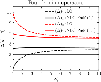
Figure 2: Extrapolations of the scaling dimensions of the two flavor-singlet four-fermion operators to $d=3$, as a function of $N_{\!f}$. In black (lower two lines) $(\Delta)_{1}$ and in red (upper two lines) $(\Delta)_{2}$. Dashed lines are the LO estimate and solid lines the NLO Padé (1,1).

Next, we comment on the relation of our result to the $1/N_{\!f}$-expansion in $d=3$. At large $N_{\!f}$, the gauged $U(1)$ current, $\overline{\psi}_{i}\gamma^{(3)}_{\mu}\psi^{i}$, is set to zero by the EOM of the gauge field, hence the operator $\mathscr{Q}_{1}$ is an EOM-vanishing operator. However, besides $\mathscr{Q}_{3}$, there still is another flavor-singlet scalar operator of dimension $4$ for $N_{\!f}=\infty$, namely $F_{\mu\nu}^{2}$. $\mathscr{Q}_{3}$ and $F_{\mu\nu}^{2}$ mix at order $1/N_{\!f}$ [11]. Looking at the $\epsilon$-expansion result in figure 2 we see that indeed only the lowest eigenvalue $(\Delta)_{1}$ (black lines) approaches $4$ for large $N_{\!f}$. The other scaling dimension (red lines) approaches $6$ as $N_{\!f}\to\infty$, implying that the two eigenoperators cannot mix at large $N_{\!f}$. This is consistent precisely because there is only one non-trivial singlet four-fermion operator at large $N_{\!f}$. Its mixing with $F_{\mu\nu}^{2}$ cannot be captured within the $\epsilon$-expansion, because the UV dimension of $F_{\mu\nu}^{2}$ differs from that of a four-fermion operator in $d=4-2\epsilon$. We can, however, test whether for any value of $\epsilon\in[0,\frac{1}{2}]$ the lowest eigenvalue $(\Delta)_{1}$, which starts off larger at $\epsilon=0$, crosses the dimension of $F_{\mu\nu}^{2}$. Such a level-crossing would require to revisit the extrapolation to $\epsilon=\frac{1}{2}$ and possibly affect the estimate. The scaling dimension of $F_{\mu\nu}^{2}$ in $\epsilon$-expansion is

$$\Delta(F^{2})=4-2\epsilon+\alpha^{2}\frac{\partial}{\partial\alpha}\left.\left(\frac{1}{\alpha^{2}}\frac{d\alpha}{d\log\mu}\right)\right|_{\alpha=\alpha^{*}}\,,$$ (5.4)

with $\alpha^{*}$ given in eq. (2.10) up to ${\cal O}(\epsilon^{4})$. At three- and four-loop order the only Padé approximation without poles in the positive real axis of $\epsilon$ is the order (2,1) and (2,2), respectively. In figure 3 we plot $(\Delta)_{1,2}$ and $\Delta(F^{2})$ as a function of $d$ for the representative cases of $N_{\!f}=1,2,$ and $10$. We observe that the only case in which $(\Delta)_{1}$ crosses $\Delta(F^{2})$ before $d=3$ is when $N_{\!f}=1$ and when we employ N²LO Padé (2,1) to predict $\Delta(F^{2})$. The N³LO Padé (2,2) prediction for $N_{\!f}=1$ does not cross $(\Delta)_{1}$ and the same holds for larger values of $N_{\!f}$. Therefore, at least at this order, $F_{\mu\nu}^{2}$ should not play a significant role in obtaining the four-fermion scaling dimension.

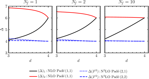
Figure 3: $\epsilon$-expansion approximations to the scaling dimensions of the two flavor-singlet four-fermion operators (black and red lines) and $F_{\mu\nu}^{2}$ (blue lines) as a function of the dimension $d$, i.e., for $\epsilon\in[0,\frac{1}{2}]$. The left, center, and right panel show the result for the representative cases of $N_{\!f}=1,2,$ and $10$, respectively. We observe that the N³LO Padé (2,2) prediction of $\Delta(F^{2})$ never crosses the NLO Padé (1,1) prediction of $(\Delta)_{1}$ in the extrapolation region.

5.3 Bilinears as ${d\to 3}$

Next we consider bilinear operators in $d=3$. In the UV, restricting to the ones without derivatives, the possibilities are

Scalar:

$$\mathcal{B}^{(0)}_{\mathrm{s}ing} =\overline{\psi}_{i}\psi^{i}\,,$$ (5.5)

$$(\,\mathcal{B}^{(0)}_{\mathrm{a}dj}\,)_{i}^{~{}j} =\overline{\psi}_{i}\psi^{j}-\frac{1}{2N_{\!f}}\overline{\psi}_{k}\psi^{k}\delta_{i}^{~{}j}\,.$$ (5.6)

The subscript refers to the representation of $SU(2N_{\!f})$. The singlet is parity-odd. We can combine parity with an element of the Cartan of $SU(2N_{\!f})$, in such a way that one component of the adjoint scalar is parity-even. Since parity squares to the identity, this Cartan element can only have $+1$ and $-1$ along the diagonal, which up to permutations we can take to be the first $N_{\!f}$, and the second $N_{\!f}$ diagonal entries, respectively. With this choice, the parity-even bilinear is $\sum_{a=1}^{N_{\!f}}(\overline{\psi}_{a}\psi^{a}-\overline{\psi}_{a+N_{\!f}}\psi^{a+N_{\!f}})$. This is the candidate to be the “chiral condensate” in QED₃ [22].

Vector:

$$\mathcal{B}^{(1)}_{{\mathrm{s}ing}~{}\mu} =\overline{\psi}_{i}\gamma^{(3)}_{\mu}\psi^{i}\,,$$ (5.7)

$$(\,\mathcal{B}^{(1)}_{{\mathrm{a}dj}~{}\mu}\,)_{i}^{~{}j} =\overline{\psi}_{i}\gamma^{(3)}_{\mu}\psi^{j}-\frac{1}{2N_{\!f}}\overline{\psi}_{k}\gamma^{(3)}_{\mu}\psi^{k}\delta_{i}^{~{}j}\,.$$ (5.8)

The singlet is the current of the gauged $U(1)$. When the interaction is turned on, it recombines with the field strength and does not flow to any primary operator of the IR CFT. The adjoint is the current that generates the $SU(2N_{\!f})$ global symmetry. Therefore, we expect it to remain conserved along the RG and flow to a conserved current of dimension $\Delta=2$ in the IR.

We now identify which $d=4-2\epsilon$ bilinears from section 4 approach the $d=3$ bilinears above. Substituting the decomposition of eqs. (2.4) and (2.5), and also using $3d$ Hodge duality, we find that

$$B^{(3)}_{\mathrm{s}ing} \quad\overset{d\to 3}{\longrightarrow}\quad\mathcal{B}^{(0)}_{\mathrm{s}ing}\,,$$ (5.9)

$$B^{(0)}_{\mathrm{a}dj},~{}B^{(3)}_{\mathrm{a}dj} \quad\overset{d\to 3}{\longrightarrow}\quad\mathcal{B}^{(0)}_{\mathrm{a}dj}\,,$$ (5.10)

$$B^{(1)}_{\mathrm{s}ing} \quad\overset{d\to 3}{\longrightarrow}\quad\mathcal{B}^{(1)}_{\mathrm{s}ing}\,,$$ (5.11)

$$B^{(1)}_{\mathrm{a}dj},~{}B^{(2)}_{\mathrm{a}dj} \quad\overset{d\to 3}{\longrightarrow}\quad\mathcal{B}^{(1)}_{\mathrm{a}dj}\,.$$ (5.12)

We denote by $\Delta(\mathcal{B})$ the scaling dimension of the operator in the IR CFT in $d=3$ that a certain bilinear $\mathcal{B}$ flows to. Therefore, we expect

$$\Delta(B^{(3)}_{\mathrm{s}ing}) \quad\overset{d\to 3}{\longrightarrow}\quad\Delta(\mathcal{B}^{(0)}_{\mathrm{s}ing})\,,$$ (5.13)

$$\Delta(B^{(0)}_{\mathrm{a}dj}),~{}\Delta(B^{(3)}_{\mathrm{a}dj}) \quad\overset{d\to 3}{\longrightarrow}\quad\Delta(\mathcal{B}^{(0)}_{\mathrm{a}dj})\,,$$ (5.14)

$$\Delta(B^{(2)}_{\mathrm{a}dj}) \quad\overset{d\to 3}{\longrightarrow}\quad 2\,.$$ (5.15)

The last equation provides a test of the $\epsilon$-expansion and the first two provide estimates of the observables $\Delta(\mathcal{B}^{(0)}_{\mathrm{s}ing})$ and $\Delta(\mathcal{B}^{(0)}_{\mathrm{a}dj})$. To this end, we employ the viable Padé approximants for $N_{\!f}=1,\dots,10$. In table 4 we list the $\epsilon$-expansion predictions at $d=3$ for $N_{\!f}=1,\dots,10$. For the cases in which the order (1,1) Padé approximant is singular, we list the fixed-order NLO prediction.

$\boldsymbol{N_{\!f}}$ $1$ $2$ $3$ $4$ $5$ $6$ $7$ $8$ $9$ $10$ $\boldsymbol{\Delta(\mathcal{B}^{(0)}_{\mathrm{s}ing})}$ $\boldsymbol{\Delta(B^{(3)}_{\mathrm{s}ing})}$ LO $2$ $2$ $2$ $2$ $2$ $2$ $2$ $2$ $2$ $2$ NLO Padé (1,1) $2.65$ $2.48$ $2.38$ $2.32$ $2.27$ $2.24$ $2.21$ $2.19$ $2.17$ $2.16$ N²LO Padé (2,1) $2.49$ $2.40$ $2.35$ $2.30$ $2.27$ $2.24$ $2.22$ $2.20$ $2.19$ $2.17$ N²LO Padé (1,2) $2.51$ $2.42$ $2.35$ $2.30$ $2.27$ $2.24$ $2.22$ $2.20$ $2.18$ $2.17$ $\boldsymbol{\Delta(\mathcal{B}^{(0)}_{\mathrm{a}dj})}$ $\boldsymbol{\Delta(B^{(0)}_{\mathrm{a}dj})}$ LO $-0.250$ $0.875$ $1.25$ $1.44$ $1.55$ $1.62$ $1.68$ $1.72$ $1.75$ $1.77$ NLO Padé (1,1) $1.32$ $1.55$ $1.67$ $1.73$ $1.78$ $1.81$ $1.83$ $1.85$ $1.87$ $1.88$ N²LO Padé (2,1) $0.238$ $1.17$ $1.48$ $1.63$ $1.72$ $1.78$ $1.82$ $1.85$ $1.87$ $1.89$ $\boldsymbol{\Delta(B^{(3)}_{\mathrm{a}dj})}$ LO $2$ $2$ $2$ $2$ $2$ $2$ $2$ $2$ $2$ $2$ NLO $0.500$ $1.25$ $1.50$ $1.62$ $1.70$ $1.75$ $1.79$ $1.81$ $1.83$ $1.85$ N²LO Padé (2,1) $1.69$ $1.75$ $1.79$ $1.81$ $1.84$ $1.85$ $1.87$ $1.88$ $1.89$ $1.90$ N²LO Padé (1,2) $1.99$ $1.95$ $1.93$ $1.92$ $1.91$ $1.91$ $1.91$ $1.92$ $1.92$ $1.92$ $\boldsymbol{\Delta(\mathcal{B}^{(1)}_{\mathrm{a}dj})}$ $\boldsymbol{\Delta(B^{(2)}_{\mathrm{a}dj})}$ LO $2.75$ $2.38$ $2.25$ $2.19$ $2.15$ $2.12$ $2.11$ $2.09$ $2.08$ $2.08$ NLO $-1.58$ $1.09$ $1.59$ $1.76$ $1.85$ $1.89$ $1.92$ $1.94$ $1.95$ $1.96$ N²LO Padé (2,1) $1.58$ $1.88$ $1.95$ $1.97$ $1.98$ $1.99$ $1.99$ $1.99$ $1.99$ $1.99$ N²LO Padé (1,2) $2.00$ $2.09$ $2.08$ $2.06$ $2.05$ $2.03$ $2.02$ $2.02$ $2.01$ $2.01$

Table 4: $\epsilon$-expansion extrapolations of scaling dimension of the $d=3$ bilinear operators $\mathcal{B}^{(0)}_{\mathrm{s}ing}$, $\mathcal{B}^{(0)}_{\mathrm{a}dj}$, and the conserved current $\mathcal{B}^{(1)}_{\mathrm{a}dj}$. In cases in which the NLO Padé (1,1) approximant is singular we list instead the values of the fixed-order NLO prediction. Only three significant digits are being displayed.

In figure 4 we plot the extrapolations for the scaling dimension of the conserved flavor-nonsinglet current $\mathcal{B}^{(1)}_{\mathrm{a}dj}$ as a function of $N_{\!f}$. We observe that both N²LO Padé approximants are closer to $2$ than the LO and NLO ones, and they remain close to $2$ even for small values of $N_{\!f}$. We consider this to be a successful test of the $\epsilon$-expansion, which supports its viability as a tool to study QED₃.

Figure 4: $\epsilon$-expansion predictions for the scaling dimension of the bilinear vector operator $\mathcal{B}^{(1)}_{\mathrm{a}dj}$ at $d=3$. The operator is associated to the conserved flavor-nonsinglet current of  $SU(2N_{\!f})$, thus its scaling dimension is expected to equal $2$. We observe that the N²LO Padé approximations are indeed close to this expectation even for small values of $N_{\!f}$.

In figure 5 we plot the various extrapolations for the scaling dimension of the two scalar operators $\mathcal{B}^{(0)}_{\mathrm{s}ing}$ and $\mathcal{B}^{(0)}_{\mathrm{a}dj}$ as a function of $N_{\!f}$. For $\mathcal{B}^{(0)}_{\mathrm{s}ing}$ we find good convergence behaviour between the NLO Padé (1,1) and the two N²LO Padé approximations. Therefore, for this observable we are able to provide a rather convincing estimate. We do stress, however, that the comparison of the various approximations does not provide rigorous error estimates, since the error due to the extrapolation is not under control. For $\mathcal{B}^{(0)}_{\mathrm{a}dj}$ we have two different operators that provide a continuation to $d=4-2\epsilon$. It is encouraging that as the order increases, the two resulting estimates approach each other. Even so, we find that for small $N_{\!f}$ the N²LO Padé approximations are spread, so the $\epsilon$-expansion at this order does not provide a definite prediction. As $N_{\!f}$ increases the situation improves, namely all NLO and N²LO approximations begin to converge.

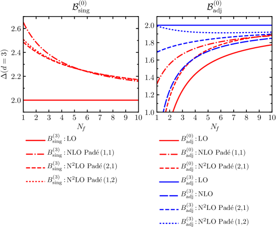
Figure 5: $\epsilon$-expansion predictions for the scaling dimension of the scalar bilinear operators $\mathcal{B}^{(0)}_{\mathrm{s}ing}$ (left panel), and $\mathcal{B}^{(0)}_{\mathrm{a}dj}$ (right panel) at $d=3$. The different colors for $\mathcal{B}^{(0)}_{\mathrm{a}dj}$ correspond to estimates from different continuations of the operator (see legend).

In table 4 we list the numerical values for the various estimates of the bilinear scaling dimensions for $N_{\!f}=1,\dots,10$.

Next, we compare to the large-$N_{\!f}$ predictions for the scaling dimensions of the bilinears. The Padé approximants used to estimate the dimensions of $\mathcal{B}^{(0)}_{\mathrm{s}ing}$ and $\mathcal{B}^{(0)}_{\mathrm{a}dj}$ do not develop a pole in the extrapolation region $0\leq\epsilon\leq\frac{1}{2}$ for any value of $N_{\!f}\geq 1$. Therefore, we can consider the approximants evaluated at $\epsilon=\frac{1}{2}$, as a function of $N_{\!f}$, expand them around $N_{\!f}=\infty$, i.e.,

$$\Delta^{\text{Pad\'{e}}}(k,l)\biggl{|}_{\epsilon=\frac{1}{2}}=2+\frac{c^{(k,l)}}{N_{\!f}}+{\cal O}(N_{\!f}^{-2})~{},$$ (5.16)

and compare the coefficient $c^{(k,l)}$ with its exact value obtained from the large-$N_{\!f}$ expansion, $c^{\text{large-}N_{\!f}}$. In what follows we use $\simeq$ to denote that we display only two significant digits.

For $\mathcal{B}^{(0)}_{\mathrm{s}ing}$, the prediction from large-$N_{\!f}$ is [5, 6]

$$\mathcal{B}^{(0)}_{\mathrm{s}ing}{:}\quad\quad\quad c^{\text{large-}N_{\!f}}=\frac{64}{3\pi^{2}}\simeq 2.2~{},$$ (5.17)

and the extrapolation obtained from the three-form singlet gives

$$B^{(3)}_{\mathrm{s}ing}{:}\quad\quad c^{(1,2)}\simeq 2.3~{},\quad c^{(2,1)}\simeq 2.4~{}.$$ (5.18)

For $\mathcal{B}^{(0)}_{\mathrm{a}dj}$, the prediction from large-$N_{\!f}$ is [4, 6]

$$\mathcal{B}^{(0)}_{\mathrm{a}dj}{:}\quad\quad\quad c^{\text{large-}N_{\!f}}=-\frac{32}{3\pi^{2}}\simeq-1.1~{},$$ (5.19)

and the extrapolations obtained from the three-form and scalar adjoints give

$$B^{(3)}_{\mathrm{a}dj}{:} \quad\quad c^{(1,2)}\simeq-1.4~{},\quad c^{(2,1)}\simeq-1.4~{},$$ (5.20)

$$B^{(0)}_{\mathrm{a}dj}{:} \quad\quad c^{(2,1)}=0~{}.$$ (5.21)

This suggests that the extrapolation of the three-form may provide a better estimate for the scaling dimension of the adjoint scalar at this order.

6 Conclusions and future directions

We employed the $\epsilon$-expansion to compute scaling dimensions of four-fermion and bilinear operators at the IR fixed point of QED in $d=4-2\epsilon$. We estimated the corresponding value for the physically interesting case of $d=3$. The results seem to confirm the expectations from the enhancement of the global symmetry as $d\to 3$ (see figures 4 and 5). Therefore, going beyond the leading order gave us more confidence that the continuation is sensible. At the same time, it appears that —with the exception of the scalar-singlet bilinear— to obtain precise estimates for the scaling dimensions for small values of $N_{\!f}$ requires even higher-order computations and perhaps more sophisticated resummation techniques (see for instance chapter $16$ of ref. [60] and references therein). The computation of such higher orders in $\epsilon$ via the standard techniques used in the present work would require hard Feynman-diagram calculations.

In recent years, several authors exploited conformal symmetry to introduce a variety of novel techniques to compute observables of the fixed point in $\epsilon$-expansion. Ref. [61] proposed an approach based on multiplet recombination, further applied and developed in refs. [62, 63, 64, 65, 66, 67, 68, 69, 70, 71, 72, 73, 74, 75, 76, 77]. Another approach is the analytic bootstrap, either together with the large-spin expansion [78], or in its Mellin-space version [79, 80, 81, 82]. Finally, ref. [83] aimed at directly computing the dilatation operator at the Wilson–Fisher fixed point. It would be interesting to attempt to apply these techniques to QED in $d=4-2\epsilon$.

On a different note, ref. [84] recently argued that QCD₃ with massless quarks undergoes a transition from a conformal IR phase, which exists for sufficiently large number of flavors, to a symmetry-breaking phase when $N_{\!f}\leq N_{\!f}^{c}$. This is analogous to the long-standing conjecture for QED₃, and so four-fermion operators may play the same role. Therefore, at least for the case of zero Chern–Simons level, $\epsilon$-expansion can be employed in a similar manner to estimate $N_{\!f}^{c}$. A LO estimate appeared in ref. [85]. In light of our results for QED₃, it would be worth studying how this estimate is modified at NLO.

Acknowledgements: we thank Joachim Brod, Martin Gorbahn, John Gracey, Igor Klebanov, Zohar Komargodski, and David Stone for their interest and the many helpful discussions. We are also indebted to the Weizmann Institute of Science, in which this research began. Research at Perimeter Institute is supported by the Government of Canada through Industry Canada and by the Province of Ontario through the Ministry of Research & Innovation.

Appendix A Feynman rules

From the QED Lagrangian in $R_{\xi}$-gauge,

$$\mathscr{L}_{\text{QED}+\text{g.f.}}=-{1\over 4}F^{\mu\nu}F_{\mu\nu}-{1\over 2\xi}(\partial_{\mu}A^{\mu})^{2}+\overline{\Psi}_{a}i\gamma^{\mu}D_{\mu}\Psi^{a}~{},$$ (A.1)

we obtain the Feynman rules

$$=\frac{i}{\not{q}}~{},$$ (A.2)

$$=-\frac{i}{q^{2}}\left(\eta^{\mu\nu}-(1-\xi)\frac{q^{\mu}q^{\nu}}{q^{2}}\right)~{},$$ (A.3)

$$=-ie\gamma^{\mu}~{}.$$ (A.4)

There is one additional counterterm coupling that we need to specify. It is a relic of the procedure with which we regulate IR divergences (see section 3.3), which essentially breaks gauge invariance. For this reason to consistently renormalize Green’s function we need to include a counterterm analogous to a mass for the photon, i.e.,

$$\parbox{113.81102pt}{\vspace*{0em}\includegraphics{./diagrams/AA_counterterm}}=-i\,\delta m_{\mathrm{I}RA}^{2}\,\eta^{\mu\nu}\,.$$ (A.5)

Only the one-loop value of $\delta m_{\mathrm{I}RA}^{2}$ enters our computations. It reads

$$\delta m_{\mathrm{I}RA}^{2}=\alpha\frac{4N_{\!f}}{\epsilon}m_{\mathrm{I}RA}^{2}+{\cal O}(\alpha^{2})\,.$$ (A.6)

To find the EOM-vanishing operators at the non-renormalizable level we apply the EOM of the fermion and photon. They read

$$\gamma^{\mu}D_{\mu}\Psi^{a}=0\,,\qquad D_{\mu}\overline{\Psi}_{a}\gamma^{\mu}=0\,,\qquad\partial^{\nu}F_{\mu\nu}+e\,\overline{\Psi}_{a}\gamma_{\mu}\Psi^{a}=0\,.$$ (A.7)

For brevity we use the shorthand notation $\gamma_{\mu}D^{\mu}\equiv\not{D}$ and use an arrow to indicate the direction in which the derivative in $\not{D}$ acts, i.e. ${\overset{\,\,\leftharpoonup}{\vphantom{a}\smash{\not{D}}}}$ and ${\overset{\,\,\rightharpoonup}{\vphantom{a}\smash{\not{D}}}}\equiv\not{D}$.

We consider the Lagrangian with additional couplings proportional to the operators introduced in section 3.1

$$\mathscr{L}=\mathscr{L}_{\text{QED}}+\sum_{i}C^{i}\mathscr{O}_{i}~{}.$$ (A.8)

To compute the Green’s function we need the Feynman rules of the operators we insert, as well as all the structures that we need to project the amplitude. For instance, to renormalize the Green’s function of $\overline{\Psi}\Psi A^{\mu}$ with one-loop insertions of $\mathscr{Q}_{1}$ we need not only the Feynman rule of $\mathscr{Q}_{1}$, but also the $\overline{\Psi}\Psi A^{\mu}$ structure of all operators that $\mathscr{Q}_{1}$ generates at one-loop.

In our case, the Feynman rules for the following three final states suffice:

$=iC^{\mathscr{O}}S_{\mathscr{O}}$      $=iC^{\mathscr{O}}\tilde{S}_{\mathscr{O}}$

$=iC^{\mathscr{O}}\hat{S}_{\mathscr{O}}$

where the structures $S_{\mathscr{O}}$, $\tilde{S}_{\mathscr{O}}$, $\hat{S}_{\mathscr{O}}$ depend on the inserted operator. For the set of operators relevant to our computation they read

$$\begin{aligned} &{\boldsymbol{S_{\mathscr{O}}}}&\mathscr{Q}_{1}&:&&2\gamma^{\mu}\otimes\gamma_{\mu}\\ &&\mathscr{Q}_{3}&:&&2\gamma^{[\mu}\gamma^{\nu}\gamma^{\rho]}\otimes\gamma_{[\mu}\gamma_{\nu}\gamma_{\rho]}\\ &&\mathscr{E}_{n}&:&&2\gamma^{[\mu_{1}}\cdots\gamma^{\mu_{n}]}\otimes\gamma_{[\mu_{1}}\cdots\gamma_{\mu_{n}]}+\epsilon a_{n}S_{\mathscr{Q}_{1}}+\epsilon b_{n}S_{\mathscr{Q}_{3}}\\ &&\mathscr{N}_{1}&:&&S_{\mathscr{Q}_{1}}\end{aligned}$$ (A.9)

$$\begin{aligned} &{\boldsymbol{\tilde{S}_{\mathscr{O}}}}&\mathscr{N}_{1}&:&&1/e\left(q^{2}\gamma^{\mu}-\not{q}q^{\mu}\right)\\ &&\mathscr{N}_{2}&:&&\tilde{S}_{\mathscr{N}_{1}}\\ &&\mathscr{N}_{3}&:&&e\left((p+q)^{2}\gamma^{\mu}-\not{q}\not{p}\gamma^{\mu}+2(\not{q}+\not{p})p^{\mu}\right)\\ &&\mathscr{N}_{4}&:&&4\not{q}\not{p}\gamma^{\mu}-4\not{q}p^{\mu}+2(2\not{p}+\not{q})q^{\mu}-2(2p\!\cdot\!q+q^{2})\gamma^{\mu}\\ &&\mathscr{P}&:&&i/e~{}m_{\mathrm{I}RA}^{2}\end{aligned}$$ (A.10)

$$\begin{aligned} &{\boldsymbol{\hat{S}_{\mathscr{O}}}}&\mathscr{N}_{2}&:&&\frac{2}{e^{2}}\left(\eta^{\mu\nu}q^{4}-q^{2}q^{\mu}q^{\nu}\right)\\ \end{aligned}$$ (A.11)

Appendix B Renormalization constants

In this appendix we list the mixing-renormalization constants of four-fermion operators. First we list the constants we need to compute the ADM of flavor-singlet four-fermion operators, which we discussed in the main text, and subsequently the constants entering the computation of the ADM of flavor-nonsinglet four-fermion operators, which we discuss in appendix C.

B.1 Flavor-singlet four-fermion operators

The divergent and finite pieces of the one-loop constants of the mixing between physical and evanescent operators are directly related to the one-loop anomalous dimension of eqs. (3.8) and (3.17) via

$$\mathcal{Z}^{(1,1)}_{\mathscr{O}\,\mathscr{O}^{\prime}}=\frac{1}{2}\gamma^{(1,0)}_{\mathscr{O}\,\mathscr{O}^{\prime}}\,, \mathcal{Z}^{(1,0)}_{\mathscr{O}\,\mathscr{O}^{\prime}}=\frac{1}{2}\gamma^{(1,-1)}_{\mathscr{O}\,\mathscr{O}^{\prime}}\,,$$ (B.1)

with $\mathscr{O},\,\mathscr{O}^{\prime}$ any physical or evanescent operator from section 3.1. To extract these constant from the $\overline{\Psi}\Psi\overline{\Psi}\Psi$ Green’s function we had to first compute the one-loop mixing of the four-fermion operators into the EOM-vanishing operator $\mathscr{N}_{1}$. For the physical operators the corresponding constants are

$$\mathcal{Z}^{(1,1)}_{\mathscr{Q}_{1}\,\mathscr{N}_{1}} =-\frac{4}{3}(2N_{\!f}+1)\,, \mathcal{Z}^{(1,0)}_{\mathscr{Q}_{1}\,\mathscr{N}_{1}} =0\,,$$ (B.2)

$$\mathcal{Z}^{(1,1)}_{\mathscr{Q}_{3}\,\mathscr{N}_{1}} =-8\,, \mathcal{Z}^{(1,0)}_{\mathscr{Q}_{3}\,\mathscr{N}_{1}} =0\,,$$ (B.3)

and for the evanescent operators they are

$$\mathcal{Z}^{(1,1)}_{\mathscr{E}_{n}\,\mathscr{N}_{1}}= 0\,, \mathcal{Z}^{(1,0)}_{\mathscr{E}_{n}\,\mathscr{N}_{1}}= -(-1)^{\frac{n(n-1)}{2}}16(n-2)(n-5)!$$

$$-\frac{4}{3}(2N_{\!f}+1)a_{n}-8b_{n}\,,$$ (B.4)

with $n$ an odd integer $\geq 5$. To compute these constants for generic $n$ we used Clifford-algebra identities from ref. [44].

As explained in section 3.2, in the computation of the mixing at two-loop level more operators enter. The only one-loop mixings entering the computation, apart from those above, is the mixing of the physical four-fermion operators into the EOM-vanishing operator $\mathscr{N}_{2}$, and the gauge-variant operator $\mathscr{P}$. The former vanish, i.e.,

$$\mathcal{Z}^{(1,1)}_{\mathscr{Q}\,\mathscr{N}_{2}}=0\,,\qquad\mathcal{Z}^{(1,0)}_{\mathscr{Q}\,\mathscr{N}_{2}}=0\,,$$ (B.5)

and the latter read

$$\mathcal{Z}^{(1,1)}_{\mathscr{Q}_{1}\,\mathscr{P}}=8N_{\!f}+4\,,\qquad\mathcal{Z}^{(1,1)}_{\mathscr{Q}_{3}\,\mathscr{P}}=4\,,\qquad\mathcal{Z}^{(1,0)}_{\mathscr{Q}\,\mathscr{P}}=0\,,$$ (B.6)

with $\mathscr{Q}=\mathscr{Q}_{1},\,\mathscr{Q}_{3}$. We do not list the corresponding constants for the evanescent operators because they do not enter the two-loop computation of the mixing of physical operators.

In table 1 we summarised on which renormalization constants the Green’s functions we computed depend on. We see that to determine the two-loop mixing of the four-fermion operators we first need to determine the two-loop mixing of the physical operators into the two EOM-vanishing operators $\mathscr{N}_{1}$ and $\mathscr{N}_{2}$. The corresponding constants read

$$\mathcal{Z}^{(2,2)}_{\mathscr{Q}_{1}\,\mathscr{N}_{2}}= \frac{8}{9}N_{\!f}(2N_{\!f}+1)\,, \mathcal{Z}^{(2,1)}_{\mathscr{Q}_{1}\,\mathscr{N}_{2}}= \frac{8}{9}N_{\!f}\,,$$ (B.7)

$$\mathcal{Z}^{(2,2)}_{\mathscr{Q}_{1}\,\mathscr{N}_{1}}= -\frac{4}{9}(12N_{\!f}^{2}+10N_{\!f}+11)\,, \mathcal{Z}^{(2,1)}_{\mathscr{Q}_{1}\,\mathscr{N}_{1}}= \frac{4}{27}(N_{\!f}+11)\,,$$ (B.8)

$$\mathcal{Z}^{(2,2)}_{\mathscr{Q}_{3}\,\mathscr{N}_{2}}= \frac{16}{3}N_{\!f}\,, \mathcal{Z}^{(2,1)}_{\mathscr{Q}_{3}\,\mathscr{N}_{2}}= \frac{32}{9}N_{\!f}\,,$$ (B.9)

$$\mathcal{Z}^{(2,2)}_{\mathscr{Q}_{3}\,\mathscr{N}_{1}}= -\frac{8}{3}(24N_{\!f}+11)\,, \mathcal{Z}^{(2,1)}_{\mathscr{Q}_{3}\,\mathscr{N}_{1}}= -\frac{8}{9}(103N_{\!f}+86)$$

$$-\frac{4}{3}a_{5}(2N_{\!f}+1)-8b_{5}\,.$$ (B.10)

Finally, the two-loop mixing constants of the two physical operators read

$$\mathcal{Z}^{(2,2)}_{\mathscr{Q}\,\mathscr{Q}^{\prime}}= \begin{bmatrix}\frac{2}{9}\left(24N_{\!f}^{2}+20N_{\!f}+103\right)&\frac{2}{3}(3N_{\!f}+1)\\ \frac{88}{3}(3N_{\!f}+1)&22\\ \end{bmatrix}\,,$$ (B.11)

$$\mathcal{Z}^{(2,1)}_{\mathscr{Q}\,\mathscr{Q}^{\prime}}= \begin{bmatrix}-\frac{1}{54}(8N_{\!f}+2275)&-\frac{1}{9}(3N_{\!f}+49)\\ \frac{4}{9}(107N_{\!f}+253)&\frac{5}{6}(8N_{\!f}+9)\\ \end{bmatrix}$$

$$+ a_{5}\begin{bmatrix}-\frac{1}{2}&0\\ \frac{2}{3}(3N_{\!f}+14)&1\\ \end{bmatrix}+b_{5}\begin{bmatrix}0&-\frac{1}{2}\\ 44&-\frac{2}{3}(N_{\!f}-12)\\ \end{bmatrix}$$

$$+ a_{7}\begin{bmatrix}0&0\\ -\frac{1}{2}&0\\ \end{bmatrix}+b_{7}\begin{bmatrix}0&0\\ 0&-\frac{1}{2}\\ \end{bmatrix}\,,$$ (B.12)

with $\mathscr{Q}=\mathscr{Q}_{1},\,\mathscr{Q}_{3}$.

B.2 Flavor-nonsinglet four-fermion operators

The renormalization of the Green’s functions with insertions of flavor-nonsinglet four-fermion operators is analogous to the one with flavor-singlets but less involved. Their flavor-off-diagonal structure forbids them to receive contributions from any EOM-vanishing or gauge-variant operator at two-loop order. Therefore, in this case we only need the mixing constants within the physical and evanescent sectors.

As in the flavor-singlet case, the one-loop mixing is directly related to the one-loop anomalous dimensions of eqs. (C.8) and (C.15) via

$$\mathcal{Z}^{(1,1)}_{\mathscr{O}\,\mathscr{O}^{\prime}}=\frac{1}{2}\gamma^{(1,0)}_{\mathscr{O}\,\mathscr{O}^{\prime}}\,, \mathcal{Z}^{(1,0)}_{\mathscr{O}\,\mathscr{O}^{\prime}}=\frac{1}{2}\gamma^{(1,-1)}_{\mathscr{O}\,\mathscr{O}^{\prime}}\,,$$ (B.13)

with $\mathscr{O},\,\mathscr{O}^{\prime}$ any physical or evanescent flavor-nonsinglet four-fermion operator; the one-loop anomalous dimensions above are given in appendix C. Finally, the two-loop mixing constants of the two physical operators read

$$\mathcal{Z}^{(2,2)}_{\mathscr{Q}\,\mathscr{Q}^{\prime}}= \begin{bmatrix}18&\frac{2}{3}N_{\!f}\\ 24N_{\!f}&18\\ \end{bmatrix}\,,$$ (B.14)

$$\mathcal{Z}^{(2,1)}_{\mathscr{Q}\,\mathscr{Q}^{\prime}}= \begin{bmatrix}-\frac{81}{2}&-\frac{1}{9}(N_{\!f}+63)\\ -4(11N_{\!f}-9)&-\frac{1}{6}(32N_{\!f}+3)\\ \end{bmatrix}$$

$$+ a_{5}\begin{bmatrix}-\frac{1}{2}&0\\ -\frac{2}{3}(N_{\!f}-12)&1\\ \end{bmatrix}+b_{5}\begin{bmatrix}0&-\frac{1}{2}\\ 36&-\frac{2}{3}(N_{\!f}-12)\\ \end{bmatrix}$$

$$+ a_{7}\begin{bmatrix}0&0\\ -\frac{1}{2}&0\\ \end{bmatrix}+b_{7}\begin{bmatrix}0&0\\ 0&-\frac{1}{2}\\ \end{bmatrix}\,,$$ (B.15)

with $\mathscr{Q}=\mathscr{Q}_{1},\,\mathscr{Q}_{3}$.

Appendix C Flavor-nonsinglet four-fermion operators

In the main part of this work we investigated bilinear and flavor-singlet four-fermion operators. There exist also four-fermion operators that are not singlets under flavor. The ones we consider in this appendix are spanned by the basis

$$\mathscr{Q}_{1} =T^{ac}_{bd}(\overline{\Psi}_{a}\gamma^{\mu}\Psi^{b})(\overline{\Psi}_{c}\gamma^{\mu}\Psi^{d})\,,$$ (C.1)

$$\mathscr{Q}_{3} =T^{ac}_{bd}(\overline{\Psi}_{a}\Gamma^{3\,\mu\nu\rho}\Psi^{b})(\overline{\Psi}_{c}\Gamma^{3}_{\mu\nu\rho}\Psi^{d})\,,$$ (C.2)

$$\mathscr{E}_{n} =T^{ac}_{bd}(\overline{\Psi}_{a}\Gamma^{n\,\mu_{1}\dots\mu_{n}}\Psi^{b})(\overline{\Psi}_{c}\Gamma^{n}_{\mu_{1}\dots\mu_{n}}\Psi^{d})+\epsilon a_{n}\mathscr{Q}_{1}+\epsilon b_{n}\mathscr{Q}_{3}\,,$$ (C.3)

with $T^{ac}_{db}=T^{ca}_{bd}$ and $T^{ac}_{ad}=T^{ab}_{bd}=0$. The computation of their ADM at one- and two-loop order entails only a subset of the Feynman diagrams needed for flavor-singlet case and is actually less involved as discussed in appendix B. In this appendix we present their ADM and their scaling dimensions at the IR fixed point in $d=4-2\epsilon$, and use this to estimate the corresponding $d=3$ observables.

$\boldsymbol{N_{\!f}}$ $1$ $2$ $3$ $4$ $5$ $6$ $7$ $8$ $9$ $10$ $\boldsymbol{(\Delta_{1})_{1}}$ $-9.00$ $-4.50$ $-3.00$ $-2.25$ $-1.80$ $-1.50$ $-1.29$ $-1.12$ $-1.00$ $-0.900$ $\boldsymbol{(\Delta_{2})_{1}}$ $35.6$ $8.53$ $3.63$ $1.95$ $1.19$ $0.782$ $0.544$ $0.393$ $0.292$ $0.221$ $\boldsymbol{(\Delta_{1})_{2}}$ $9.00$ $4.50$ $3.00$ $2.25$ $1.80$ $1.50$ $1.29$ $1.12$ $1.00$ $0.900$ $\boldsymbol{(\Delta_{2})_{2}}$ $-101$ $-29.3$ $-14.9$ $-9.40$ $-6.67$ $-5.09$ $-4.08$ $-3.38$ $-2.87$ $-2.49$

Table 5: Three significant digits of the one-loop, $(\Delta_{1})_{i}$, and the two-loop, $(\Delta_{2})_{i}$, contributions to the scaling dimension of the flavor-nonsinglet four-fermion operators for various cases of $N_{\!f}$. To obtain the two-loop $(\Delta_{2})_{i}$ values we implemented the algorithm to include the effect of evanescent operators [30].

In the flavor scheme, the full one-loop ADM of the physical and evanescent operators and the two-loop entries required read:

$$\gamma^{(1,0)}_{nm} =\left\{\begin{array}[]{cl}2n(n-1)(n-5)(n-6)&\text{for}\quad m=n-2\\ -4(n-1)(n-3)&\text{for}\quad m=n\\ 2&\text{for}\quad m=n+2\\ 0&\text{otherwise\,,}\\ \end{array}\right.$$ (C.8)

$$\gamma^{(1,-1)}_{nm} =\left\{\begin{array}[]{ll}-2n(n-1)(n-5)(n-6)a_{n-2}\\ \quad+4(n-1)(n-3)a_{n}-2a_{n+2}+72b_{n}&\text{for}~{}m=1,\,n\geq 5\\[10.00002pt] -80\delta_{n5}\\ \quad-2n(n-1)(n-5)(n-6)b_{n-2}\\ \qquad+4(n-1)(n-3)b_{n}-2b_{n+2}+2a_{n}&\text{for}~{}m=3,\,n\geq 5\\[10.00002pt] \hskip 70.0001pt0&\text{otherwise\,,}\end{array}\right.$$ (C.15)

$$\gamma^{(2,0)}_{nm} =\left\{\begin{array}[]{ll}\begin{bmatrix}-162&-28-\frac{4}{9}N_{\!f}\\ 144-176N_{\!f}&78-\frac{64}{3}N_{\!f}\end{bmatrix}+&\\ +a_{5}\begin{bmatrix}-2&0\\ -\frac{8}{3}N_{\!f}&2\\ \end{bmatrix}+b_{5}\begin{bmatrix}0&-2\\ 72&-\frac{8}{3}N_{\!f}\\ \end{bmatrix}&\text{for}~{}n,m=1,3\\[20.00003pt] \hskip 70.0001pt0&\text{for}~{}n\geq 5\text{ and }m=1,3\\[10.00002pt] \hskip 50.00008pt\text{not required}&\text{otherwise}\,.\end{array}\right.$$ (C.20)

The part of the one-loop result that does not depend on $a_{n}$ and $b_{n}$ was first computed in ref. [48].

Next we evaluate these ADMs at the fixed point

$$(\gamma_{1}^{*})_{nm} =\frac{3}{2N_{\!f}}\times\left\{\begin{array}[]{cl}n(n-1)(n-5)(n-6)&\text{for}\quad m=n-2\\ -2(n-1)(n-3)&\text{for}\quad m=n\\ 1&\text{for}\quad m=n+2\\ 0&\text{otherwise\,.}\end{array}\right.$$ (C.25)

$$(\gamma_{2}^{*})_{nm} =\left\{\begin{array}[]{ll}-\frac{1}{8N_{\!f}^{2}}\begin{bmatrix}729&153+2N_{\!f}\\ 324+792N_{\!f}&-351+96N_{\!f}\end{bmatrix}&\\ +\frac{3}{8N_{\!f}^{2}}a_{5}\begin{bmatrix}-3&0\\ -4N_{\!f}&3\end{bmatrix}+\frac{3}{8N_{\!f}^{2}}b_{5}\begin{bmatrix}0&-3\\ 108&-4N_{\!f}\end{bmatrix}&\text{for}\quad n,m=1,3\,,\\[20.00003pt] \frac{3}{2N_{\!f}}\left(-n(n-1)(n-5)(n-6)a_{n-2}\right.\\ \left.\qquad+2(n-1)(n-3)a_{n}-a_{n+2}+36b_{n}\right)&\text{for}~{}m=1,\,n\geq 5~{},\\[10.00002pt] -\frac{60}{N_{\!f}}\delta_{n5}\\ \quad+\frac{3}{2N_{\!f}}\left(-n(n-1)(n-5)(n-6)b_{n-2}\right.\\ \qquad\left.+2(n-1)(n-3)b_{n}-b_{n+2}+a_{n}\right)&\text{for}~{}m=3,\,n\geq 5~{},\\[10.00002pt] \hskip 50.00008pt\text{not required}&\text{otherwise\,.}\end{array}\right.$$ (C.34)

Following ref. [30] we shift to the scheme in which the physical–physical subblock forms an invariant subspace. In this scheme we are able to extract the scheme-independent ${\cal O}(\epsilon^{2})$ corrections to the scaling dimensions, i.e., the $(\Delta_{2})_{i}$s. In table 5 we list the values for the representative cases of $N_{\!f}=1,\dots,10$ and in table 6 the LO and NLO predictions for the scaling dimensions at $d=3$. The NLO Padé (1,1) prediction of scaling dimension $(\Delta)_{2}$ contains poles in the extrapolation region $\epsilon\in[0,\frac{1}{2}]$, so we list the fixed-order NLO prediction instead.

$\boldsymbol{N_{\!f}}$ $1$ $2$ $3$ $4$ $5$ $6$ $7$ $8$ $9$ $10$ $\boldsymbol{(\Delta)_{1}}$ LO $-0.500$ $1.75$ $2.50$ $2.88$ $3.10$ $3.25$ $3.36$ $3.44$ $3.50$ $3.55$ NLO Padé (1,1) $3.26$ $3.17$ $3.22$ $3.30$ $3.37$ $3.43$ $3.49$ $3.53$ $3.57$ $3.60$ $\boldsymbol{(\Delta)_{2}}$ LO $8.50$ $6.25$ $5.50$ $5.12$ $4.90$ $4.75$ $4.64$ $4.56$ $4.50$ $4.45$ NLO $-16.7$ $-1.09$ $1.78$ $2.78$ $3.23$ $3.48$ $3.62$ $3.72$ $3.78$ $3.83$

Table 6: LO and either NLO Padé (1,1) or fixed-order NLO predictions for the scaling dimension of the two flavor-nonsinglet four-fermion operators at $d=3$ for various values of $N_{\!f}$. Only three significant digits are being displayed.

References

• [1] J. A. Gracey, Electron mass anomalous dimension at $O(1/N_{f}^{2})$ in quantum electrodynamics, Phys. Lett. B317 (1993) 415–420, [hep-th/9309092].
• [2] J. A. Gracey, Computation of critical exponent $eta$ at $O(1/N_{f}^{2})$ in quantum electrodynamics in arbitrary dimensions, Nucl. Phys. B414 (1994) 614–648, [hep-th/9312055].
• [3] W. Rantner and X.-G. Wen, Spin correlations in the algebraic spin liquid: Implications for high-${T}_{c}$ superconductors, Phys. Rev. B 66 (Oct, 2002) 144501.
• [4] M. Hermele, T. Senthil, and M. P. A. Fisher, Algebraic spin liquid as the mother of many competing orders, Phys. Rev. B 72 (Sep, 2005) 104404.
• [5] M. Hermele, T. Senthil, and M. P. A. Fisher, Erratum: Algebraic spin liquid as the mother of many competing orders [phys. rev. b 72, 104404 (2005)], Phys. Rev. B 76 (Oct, 2007) 149906.
• [6] R. K. Kaul and S. Sachdev, Quantum criticality of u(1) gauge theories with fermionic and bosonic matter in two spatial dimensions, Phys. Rev. B 77 (Apr, 2008) 155105.
• [7] C. Xu, Renormalization group studies on four-fermion interaction instabilities on algebraic spin liquids, Phys. Rev. B 78 (Aug, 2008) 054432.
• [8] V. Borokhov, A. Kapustin, and X.-k. Wu, Topological disorder operators in three-dimensional conformal field theory, JHEP 11 (2002) 049, [hep-th/0206054].
• [9] S. S. Pufu, Anomalous dimensions of monopole operators in three-dimensional quantum electrodynamics, Phys. Rev. D89 (2014), no. 6 065016, [arXiv:1303.6125].
• [10] E. Dyer, M. Mezei, and S. S. Pufu, Monopole Taxonomy in Three-Dimensional Conformal Field Theories, arXiv:1309.1160.
• [11] S. M. Chester and S. S. Pufu, Anomalous dimensions of scalar operators in QED3, JHEP 08 (2016) 069, [arXiv:1603.05582].
• [12] Y. Huh and P. Strack, Stress tensor and current correlators of interacting conformal field theories in 2+1 dimensions: Fermionic Dirac matter coupled to U(1) gauge field, JHEP 01 (2015) 147, [arXiv:1410.1902]. [Erratum: JHEP03,054(2016)].
• [13] Y. Huh, P. Strack, and S. Sachdev, Conserved current correlators of conformal field theories in 2+1 dimensions, Phys. Rev. B88 (2013) 155109, [arXiv:1307.6863]. [Erratum: Phys. Rev.B90,no.19,199902(2014)].
• [14] S. Giombi, G. Tarnopolsky, and I. R. Klebanov, On $C_{J}$ and $C_{T}$ in Conformal QED, JHEP 08 (2016) 156, [arXiv:1602.01076].
• [15] I. R. Klebanov, S. S. Pufu, S. Sachdev, and B. R. Safdi, Entanglement Entropy of 3-d Conformal Gauge Theories with Many Flavors, JHEP 05 (2012) 036, [arXiv:1112.5342].
• [16] S. M. Chester and S. S. Pufu, Towards bootstrapping QED3, JHEP 08 (2016) 019, [arXiv:1601.03476].
• [17] K. G. Wilson and M. E. Fisher, Critical exponents in 3.99 dimensions, Phys. Rev. Lett. 28 (1972) 240–243.
• [18] L. Di Pietro, Z. Komargodski, I. Shamir, and E. Stamou, Quantum Electrodynamics in $d=3$ from the $\epsilon$ Expansion, Phys. Rev. Lett. 116 (2016), no. 13 131601, [arXiv:1508.06278].
• [19] S. M. Chester, M. Mezei, S. S. Pufu, and I. Yaakov, Monopole operators from the $4-\epsilon$ expansion, JHEP 12 (2016) 015, [arXiv:1511.07108].
• [20] S. Giombi, I. R. Klebanov, and G. Tarnopolsky, Conformal QEDd, $F$-Theorem and the $\epsilon$ Expansion, J. Phys. A49 (2016), no. 13 135403, [arXiv:1508.06354].
• [21] R. D. Pisarski, Chiral Symmetry Breaking in Three-Dimensional Electrodynamics, Phys. Rev. D29 (1984) 2423.
• [22] C. Vafa and E. Witten, Eigenvalue Inequalities for Fermions in Gauge Theories, Commun.Math.Phys. 95 (1984) 257.
• [23] T. Appelquist, D. Nash, and L. C. R. Wijewardhana, Critical Behavior in (2+1)-Dimensional QED, Phys. Rev. Lett. 60 (1988) 2575.
• [24] T. Appelquist and L. C. R. Wijewardhana, Phase structure of noncompact QED3 and the Abelian Higgs model, in Proceedings, 3rd International Symposium on Quantum theory and symmetries (QTS3): Cincinnati, USA, September 10-14, 2003, pp. 177–191, 2004. hep-ph/0403250.
• [25] K. Kaveh and I. F. Herbut, Chiral symmetry breaking in QED(3) in presence of irrelevant interactions: A Renormalization group study, Phys. Rev. B71 (2005) 184519, [cond-mat/0411594].
• [26] J. Braun, H. Gies, L. Janssen, and D. Roscher, Phase structure of many-flavor QED3, Phys. Rev. D90 (2014), no. 3 036002, [arXiv:1404.1362].
• [27] D. B. Kaplan, J.-W. Lee, D. T. Son, and M. A. Stephanov, Conformality Lost, Phys. Rev. D80 (2009) 125005, [arXiv:0905.4752].
• [28] S. Gukov, RG Flows and Bifurcations, arXiv:1608.06638.
• [29] L. Janssen and Y.-C. He, Critical behavior of the QED3-Gross-Neveu model: duality and deconfined criticality, arXiv:1708.02256.
• [30] L. Di Pietro and E. Stamou, Operator mixing in $\epsilon$-expansion: scheme and evanescent (in)dependence.
• [31] A. Karch, B. Robinson, and D. Tong, More Abelian Dualities in 2+1 Dimensions, JHEP 01 (2017) 017, [arXiv:1609.04012].
• [32] P.-S. Hsin and N. Seiberg, Level/rank Duality and Chern-Simons-Matter Theories, JHEP 09 (2016) 095, [arXiv:1607.07457].
• [33] F. Benini, P.-S. Hsin, and N. Seiberg, Comments on global symmetries, anomalies, and duality in (2 + 1)d, JHEP 04 (2017) 135, [arXiv:1702.07035].
• [34] O. Aharony, Baryons, monopoles and dualities in Chern-Simons-matter theories, JHEP 02 (2016) 093, [arXiv:1512.00161].
• [35] A. Karch and D. Tong, Particle-Vortex Duality from 3d Bosonization, Phys. Rev. X6 (2016), no. 3 031043, [arXiv:1606.01893].
• [36] J. Murugan and H. Nastase, Particle-vortex duality in topological insulators and superconductors, JHEP 05 (2017) 159, [arXiv:1606.01912].
• [37] N. Seiberg, T. Senthil, C. Wang, and E. Witten, A Duality Web in 2+1 Dimensions and Condensed Matter Physics, Annals Phys. 374 (2016) 395–433, [arXiv:1606.01989].
• [38] C. Xu and Y.-Z. You, Self-dual Quantum Electrodynamics as Boundary State of the three dimensional Bosonic Topological Insulator, Phys. Rev. B92 (2015), no. 22 220416, [arXiv:1510.06032].
• [39] N. Karthik and R. Narayanan, No evidence for bilinear condensate in parity-invariant three-dimensional QED with massless fermions, Phys. Rev. D93 (2016), no. 4 045020, [arXiv:1512.02993].
• [40] S. J. Hands, J. B. Kogut, L. Scorzato, and C. G. Strouthos, The Chiral limit of noncompact QED in three-dimensions, Nucl. Phys. Proc. Suppl. 119 (2003) 974–976, [hep-lat/0209133]. [,974(2002)].
• [41] S. J. Hands, J. B. Kogut, L. Scorzato, and C. G. Strouthos, Non-compact QED(3) with N(f) = 1 and N(f) = 4, Phys. Rev. B70 (2004) 104501, [hep-lat/0404013].
• [42] C. Strouthos and J. B. Kogut, Chiral Symmetry breaking in Three Dimensional QED, J.Phys.Conf.Ser. 150 (2009) 052247, [arXiv:0808.2714].
• [43] J. A. Gracey, Three loop MS-bar tensor current anomalous dimension in QCD, Phys. Lett. B488 (2000) 175–181, [hep-ph/0007171].
• [44] A. D. Kennedy, Clifford Algebras in Two $\omega$ Dimensions, J. Math. Phys. 22 (1981) 1330–1337.
• [45] J. C. Collins, Renormalization, vol. 26 of Cambridge Monographs on Mathematical Physics. Cambridge University Press, Cambridge, 1986.
• [46] S. G. Gorishnii, A. L. Kataev, and S. A. Larin, Analytical Four Loop Result for Beta Function in QED in Ms and Mom Schemes, Phys. Lett. B194 (1987) 429–432.
• [47] S. G. Gorishnii, A. L. Kataev, S. A. Larin, and L. R. Surguladze, The Analytical four loop corrections to the QED Beta function in the MS scheme and to the QED psi function: Total reevaluation, Phys. Lett. B256 (1991) 81–86.
• [48] M. J. Dugan and B. Grinstein, On the vanishing of evanescent operators, Phys. Lett. B256 (1991) 239–244.
• [49] A. Bondi, G. Curci, G. Paffuti, and P. Rossi, Ultraviolet Properties of the Generalized Thirring Model With U($N$) Symmetry, Phys. Lett. B216 (1989) 345–348.
• [50] M. Beneke and V. A. Smirnov, Ultraviolet renormalons in Abelian gauge theories, Nucl. Phys. B472 (1996) 529–590, [hep-ph/9510437].
• [51] S. Herrlich and U. Nierste, Evanescent operators, scheme dependences and double insertions, Nucl. Phys. B455 (1995) 39–58, [hep-ph/9412375].
• [52] L. D. Faddeev and V. N. Popov, Feynman Diagrams for the Yang-Mills Field, Phys. Lett. B25 (1967) 29–30.
• [53] M. Misiak and M. Munz, Two loop mixing of dimension five flavor changing operators, Phys. Lett. B344 (1995) 308–318, [hep-ph/9409454].
• [54] K. G. Chetyrkin, M. Misiak, and M. Munz, Beta functions and anomalous dimensions up to three loops, Nucl. Phys. B518 (1998) 473–494, [hep-ph/9711266].
• [55] P. Nogueira, Automatic Feynman graph generation, J.Comput.Phys. 105 (1993) 279–289.
• [56] J. Kuipers, T. Ueda, J. Vermaseren, and J. Vollinga, FORM version 4.0, Comput.Phys.Commun. 184 (2013) 1453–1467, [arXiv:1203.6543].
• [57] C. Bobeth, M. Misiak, and J. Urban, Photonic penguins at two loops and $m_{t}$ dependence of $BR[B\to X_{s}\ell^{+}\ell^{-}]$, Nucl. Phys. B574 (2000) 291–330, [hep-ph/9910220].
• [58] G. ’t Hooft and M. J. G. Veltman, Regularization and Renormalization of Gauge Fields, Nucl. Phys. B44 (1972) 189–213.
• [59] P. Breitenlohner and D. Maison, Dimensional Renormalization and the Action Principle, Commun. Math. Phys. 52 (1977) 11–38.
• [60] H. Kleinert and V. Schulte-Frohlinde, Critical properties of phi**4-theories. 2001.
• [61] S. Rychkov and Z. M. Tan, The $\epsilon$-expansion from conformal field theory, J. Phys. A48 (2015), no. 29 29FT01, [arXiv:1505.00963].
• [62] P. Basu and C. Krishnan, $\epsilon$-expansions near three dimensions from conformal field theory, JHEP 11 (2015) 040, [arXiv:1506.06616].
• [63] S. Ghosh, R. K. Gupta, K. Jaswin, and A. A. Nizami, $\epsilon$-Expansion in the Gross-Neveu Model from Conformal Field Theory, arXiv:1510.04887.
• [64] A. Raju, $\epsilon$-Expansion in the Gross-Neveu CFT, arXiv:1510.05287.
• [65] E. D. Skvortsov, On (Un)Broken Higher-Spin Symmetry in Vector Models, in Proceedings, International Workshop on Higher Spin Gauge Theories: Singapore, Singapore, November 4-6, 2015, pp. 103–137, 2017. arXiv:1512.05994.
• [66] S. Giombi and V. Kirilin, Anomalous dimensions in CFT with weakly broken higher spin symmetry, JHEP 11 (2016) 068, [arXiv:1601.01310].
• [67] K. Nii, Classical equation of motion and Anomalous dimensions at leading order, JHEP 07 (2016) 107, [arXiv:1605.08868].
• [68] S. Yamaguchi, The $\epsilon$-expansion of the codimension two twist defect from conformal field theory, PTEP 2016 (2016), no. 9 091B01, [arXiv:1607.05551].
• [69] V. Bashmakov, M. Bertolini, and H. Raj, Broken current anomalous dimensions, conformal manifolds, and renormalization group flows, Phys. Rev. D95 (2017), no. 6 066011, [arXiv:1609.09820].
• [70] C. Hasegawa and Yu. Nakayama, $\epsilon$-Expansion in Critical $\phi^{3}$-Theory on Real Projective Space from Conformal Field Theory, Mod. Phys. Lett. A32 (2017), no. 07 1750045, [arXiv:1611.06373].
• [71] K. Roumpedakis, Leading Order Anomalous Dimensions at the Wilson-Fisher Fixed Point from CFT, JHEP 07 (2017) 109, [arXiv:1612.08115].
• [72] S. Giombi, V. Kirilin, and E. Skvortsov, Notes on Spinning Operators in Fermionic CFT, JHEP 05 (2017) 041, [arXiv:1701.06997].
• [73] F. Gliozzi, A. L. Guerrieri, A. C. Petkou, and C. Wen, Generalized wilson-fisher critical points from the conformal operator product expansion, Phys. Rev. Lett. 118 (Feb, 2017) 061601.
• [74] F. Gliozzi, A. L. Guerrieri, A. C. Petkou, and C. Wen, The analytic structure of conformal blocks and the generalized Wilson-Fisher fixed points, JHEP 04 (2017) 056, [arXiv:1702.03938].
• [75] A. Codello, M. Safari, G. P. Vacca, and O. Zanusso, Leading CFT constraints on multi-critical models in $d>2$, JHEP 04 (2017) 127, [arXiv:1703.04830].
• [76] C. Behan, L. Rastelli, S. Rychkov, and B. Zan, Long-range critical exponents near the short-range crossover, Phys. Rev. Lett. 118 (2017), no. 24 241601, [arXiv:1703.03430].
• [77] C. Behan, L. Rastelli, S. Rychkov, and B. Zan, A scaling theory for the long-range to short-range crossover and an infrared duality, arXiv:1703.05325.
• [78] L. F. Alday, Solving CFTs with Weakly Broken Higher Spin Symmetry, arXiv:1612.00696.
• [79] K. Sen and A. Sinha, On critical exponents without Feynman diagrams, J. Phys. A49 (2016), no. 44 445401, [arXiv:1510.07770].
• [80] R. Gopakumar, A. Kaviraj, K. Sen, and A. Sinha, Conformal Bootstrap in Mellin Space, Phys. Rev. Lett. 118 (2017), no. 8 081601, [arXiv:1609.00572].
• [81] R. Gopakumar, A. Kaviraj, K. Sen, and A. Sinha, A Mellin space approach to the conformal bootstrap, JHEP 05 (2017) 027, [arXiv:1611.08407].
• [82] P. Dey, A. Kaviraj, and A. Sinha, Mellin space bootstrap for global symmetry, JHEP 07 (2017) 019, [arXiv:1612.05032].
• [83] P. Liendo, Revisiting the dilatation operator of the Wilson-Fisher fixed point, Nucl. Phys. B920 (2017) 368–384, [arXiv:1701.04830].
• [84] Z. Komargodski and N. Seiberg, A Symmetry Breaking Scenario for QCD3, arXiv:1706.08755.
• [85] H. Goldman and M. Mulligan, Stability of $SU(N_{c})$ QCD3 from the $\epsilon$-Expansion, Phys. Rev. D94 (2016), no. 6 065031, [arXiv:1606.07067].