Operator mixing in $\boldsymbol{\epsilon}$-expansion
Scheme and evanescent (in)dependence

Abstract

We consider theories with fermionic degrees of freedom that have a fixed point of Wilson–Fisher type in non-integer dimension $d=4-2\epsilon$. Due to the presence of evanescent operators, i.e., operators that vanish in integer dimensions, these theories contain families of infinitely many operators that can mix with each other under renormalization. We clarify the dependence of the corresponding anomalous-dimension matrix on the choice of renormalization scheme beyond leading order in $\epsilon$-expansion. In standard choices of scheme, we find that eigenvalues at the fixed point cannot be extracted from a finite-dimensional block. We illustrate in examples a truncation approach to compute the eigenvalues. These are observable scaling dimensions, and, indeed, we find that the dependence on the choice of scheme cancels. As an application, we obtain the IR scaling dimension of four-fermion operators in QED in $d=4-2\epsilon$ at order ${\cal O}(\epsilon^{2})$.

tableofcontents.1tableofcontents.1Table of ContentsTable of Contentstableofcontents.1

1 Introduction

One of the tools to study conformal field theories (CFTs) is to realize them as the endpoint of a renormalization group (RG) flow. Starting from a description in terms of a weakly-coupled UV Lagrangian deformed by a relevant coupling, the dimension $d$ of space(-time) can be continued close to the upper-critical value $d_{c}$, in which the IR and the free UV fixed points coalesce. When $d=d_{c}-2\epsilon$ with $\epsilon\ll 1$, the observables of the IR CFT admit a systematic expansion in the parameter $\epsilon$ [1, 2]. Eventually, an extrapolation to $\epsilon$ of ${\cal O}(1)$ is attempted in order to estimate observables of the original strongly-coupled CFT.

A known property of the dimensional continuation is that the spectrum of operators is enlarged, i.e., in $d=d_{c}-2\epsilon$ there exist so-called evanescent operators that become redundant when $\epsilon\to 0$. These operators are more than a mere curiosity: as a consequence of their existence, the fixed points in non-integer $d$ have qualitatively new features compared to the standard, integer-dimensional CFTs that they continue. For instance, it was shown in refs. [8, 9] that in theories of free bosons and $\phi^{4}$-theories evanescent operators lead to negative-norm states in radial quantization, implying that the fixed point in non-integer dimension is not unitary. These negative norm states have large scaling dimensions, so in the example considered in ref. [8, 9] the evanescent operators do not affect the properties of the light spectrum.

The departure from standard CFTs is even more pronounced in theories with fermionic degrees of freedom, due to the fact that theories with free fermions in non-integer dimension contain infinitely many evanescent operators with the same scaling dimension and spin. One way to construct them is by antisymmetrizing $n$ gamma matrices, where $n$ runs over the positive integers, such that they vanish in integer $d<n$. The simplest example is that of the scalar four-fermion operators

$$\mathscr{O}_{n}=(\overline{\Psi}\Gamma^{n}_{\mu_{1}\dots\mu_{n}}\Psi)^{2}~{},\quad\text{with}\quad\Gamma^{n}_{\mu_{1}\dots\mu_{n}}\equiv\gamma_{[\mu_{1}}\dots\gamma_{\mu_{n}]}~{},$$ (1.1)

where the square brackets denote antisymmetrization. When interactions are turned on, all these operators can mix with each other. These mixings result in an anomalous-dimension matrix (ADM) of infinite size, which makes the computation of the eigenvalues a considerably more involved problem than in the bosonic case.

At leading order (LO), there is a drastic simplification, because the operators that are not evanescent —the so-called physical operators— form a finite-dimensional invariant subspace under mixing, i.e., the evanescent–physical entries of the LO ADM vanish. Therefore, the IR scaling dimensions of the physical operators at LO in $\epsilon$ can be obtained by diagonalizing a finite-size matrix. At next-to-leading order (NLO) and beyond, the ADM is scheme-dependent. In the context of $d=4$ computations within dimensional regularization, refs. [10, 11] introduced a scheme choice with the attractive property that the block form of the LO ADM is preserved at all orders. The same scheme was proposed in refs. [12, 13] in the context of $d=2$ Gross–Neveu/Thirring models, though formulated in a different language.

In this paper we investigate the problem of obtaining the IR scaling dimension of physical operators beyond LO in $\epsilon$ when there is mixing with infinitely many evanescent operators. Naively, the scheme choice of ref. [10, 11, 12, 13] seems to trivialize the problem by restricting it to the finite-dimensional invariant subspace spanned by physical operators. However, this leads to an apparent paradox, because the entries of the finite-size block of the ADM do not transform properly under a change of basis. For instance, they are affected by redefinitions of the evanescent operators by a multiple of $\epsilon\times$the physical operators [14]. This can be interpreted as a sign of renormalization-scheme dependence.

We resolve this issue by studying the transformation rules of the ADM under a change of scheme, keeping $\epsilon\neq 0$. The general transformation rule turns out to depend on $\epsilon$. We demonstrate how this $\epsilon$ dependence is important to ensure that the eigenvalues at the fixed point are invariant under a change of scheme. In particular, we show that going from the minimal subtraction ($\overline{\mathrm{M}S}$) scheme to the scheme used for evanescent operators in ref. [10, 11, 12, 13] introduces terms of order $\epsilon$ in the one-loop ADM. At the fixed point, these terms spoil the block structure of the ADM at ${\cal O}(\epsilon^{2})$. Therefore, the finite-size physical block of the two-loop ADM is not sufficient by itself to extract the scaling dimensions at NLO. The additional input required is the full one-loop mixing of the infinite tower of evanescent operators into the physical operators. Once this is known, one can finally compute the finitely many eigenvalues associated to the physical operators. This requires a rotation or, equivalently, a further change of scheme that completely fixes the aforementioned ambiguity in the choice of basis for the evanescent operators. We illustrate the procedure by carrying it out explicitly in the example of four-fermion operators in QED in $d=4-2\epsilon$. After computing all the relevant entries of the ADM up to order $\epsilon^{2}$, we approximate the first two eigenvalues by truncating to a finite number of evanescent operators. We test that the approximations converge as we increase the truncation.

There are several examples of CFTs with fermionic degrees of freedom that can be studied in $\epsilon$-expansion and to which the method we describe here is applicable, see for instance the recent works [16, 17, 18, 15, 19, 20, 21, 22, 23, 24, 25, 26] and references therein. In our companion paper [27], we focus on $3d$ QED and use the NLO eigenvalues obtained here to estimate the scaling dimensions of four-fermion operators in $d=3$.

The rest of the paper is organized as follows: in section 2 we review the general setup of the $\epsilon$-expansion, fix our notation, and relate the CFT scaling dimensions at NLO to renormalization constants; in section 3 we discuss the transformation rules of the beta function and the ADM under a change of renormalization scheme, first to all orders in perturbation theory and then more explicitly at the two-loop order, illustrating the scheme-independence of the scaling dimensions; in section 4 we explain the block structure of the mixing between evanescent and physical operators and show that neither in $\overline{\mathrm{M}S}$ nor in the scheme of ref. [10, 11, 12, 13] does the ADM at the fixed point have an invariant subspace at NLO; in section 5 we work out the example of four-fermion operators in QED and introduce the truncation algorithm that allows us to compute the scaling dimensions at the fixed point. Supplementary material and formulas for the anomalous dimensions computed in ref. [27] are collected in the appendices.

2 Fixed points and scaling dimensions in $\boldsymbol{d=4-2\epsilon}$

Consider a theory in $d=4$ that admits a perturbative expansion in a classically marginal coupling $\alpha$. For $\alpha=0$ the theory is free; its local operators are products of the fields and their derivatives, and their correlators are given by Wick contractions. When the interaction is turned on, we can compute corrections to the correlators in a perturbative expansion in $\alpha$. Each order in this expansion can be continued to a non-integer value of the dimension $d$ [2, 28]. Upon continuation to $d\neq 4$, the coupling acquires a nonzero mass dimension. For definiteness we keep in mind the example of gauge theories, where $\alpha=\frac{g^{2}}{16\pi^{2}}$, and take this acquired mass dimension to be $4-d\equiv 2\epsilon$.

Correlators of local operators have poles at $\epsilon=0$, which can be subtracted by defining the renormalized coupling and the renormalized operators as

$$\alpha_{0} =Z_{\alpha}\alpha(\mu)\mu^{2\epsilon}~{},$$ (2.1)

$$(\mathscr{O}_{0})_{i} =(\mathcal{Z}^{-1})_{i}^{~{}j}\mathscr{O}_{j}~{}.$$ (2.2)

The subscript “0” labels bare quantities. $Z_{\alpha}$ and $(\mathcal{Z}^{-1})_{i}^{~{}j}$ are the renormalization constants that subtract the divergences. We stress that here we are interested in the dynamics for $\epsilon\neq 0$. Therefore, the procedure of absorbing the divergences in $Z_{\alpha}$ and $(\mathcal{Z}^{-1})_{i}^{~{}j}$ is just an efficient way to keep track of the leading behavior of correlators for $\epsilon\ll 1$. This observation also appeared recently in ref. [29], see also section $1.35$ of ref. [30].

In the perturbative expansion of the renormalization constants in $\alpha$, each term admits an additional Laurent expansion in $\epsilon$, i.e.,

$$Z_{\alpha}(\alpha,\epsilon)=1+\sum_{L=1}^{\infty}\alpha^{L}\sum_{M=-L}^{\infty}\epsilon^{M}Z_{\alpha}^{(L,-M)}~{},$$ (2.3)

$$\mathcal{Z}(\alpha,\epsilon)=\mathbb{1}+\sum_{L=1}^{\infty}\alpha^{L}\sum_{M=-L}^{\infty}\epsilon^{M}\mathcal{Z}^{(L,-M)}~{}.$$ (2.4)

Different choices of the terms that are finite for $\epsilon\to 0$ correspond to different (mass-independent) renormalization schemes. A standard choice is the $\overline{\mathrm{M}S}$ scheme, in which these finite terms are set to zero. When evanescent operators are present, it is more convenient to use a different scheme that includes some specific finite terms $\mathcal{Z}^{(L,0)}$ We discuss this in detail below. For the moment, we keep the scheme generic.

From the renormalization constants one obtains the RG functions, namely the beta function and the ADM. The beta function determines the running of the coupling $\alpha$

$$\frac{d\alpha}{d\log\mu}=-2\epsilon\alpha+\beta(\alpha,\epsilon)~{}.$$ (2.5)

A convenient way to define the ADM is to consider the theory deformed by adding new couplings proportional to composite operators

$$\mathscr{L}\to\mathscr{L}+(C_{0})^{i}(\mathscr{O}_{0})_{i}~{}.$$ (2.6)

The ADM, $\gamma$, is defined as the running of the couplings $C^{i}$ to linear order in them, namely

$${\gamma(\alpha,\epsilon)}_{j}^{~{}i}\equiv\frac{\partial}{\partial C^{j}}\left.\left(\frac{dC^{i}}{d\log\mu}\right)\right|_{C=0}\,.$$ (2.7)

It then follows from eq. (2.2) that the renormalized couplings $C^{i}$ are related to the bare ones via

$$(C_{0})^{j}=C^{i}\mathcal{Z}_{i}^{~{}j}~{}.$$ (2.8)

From the fact that bare quantities do not depend on the renormalization scale $\mu$, we obtain via eqs. (2.5) and (2.7) the standard formulas

$$\beta(\alpha,\epsilon) =-\alpha\frac{d\,\log Z_{\alpha}}{d\log\mu}\equiv-2\alpha\sum_{L=1}^{\infty}\alpha^{L}\beta^{(L)}~{},$$ (2.9)

$${\gamma(\alpha,\epsilon)} =-\frac{d\log\mathcal{Z}}{d\log\mu}\equiv\sum_{L=1}^{\infty}\alpha^{L}\gamma^{(L)}~{}.$$ (2.10)

In schemes in which finite terms $Z_{\alpha}^{(L,M)}$ and $\mathcal{Z}^{(L,M)}$ with $M\leq 0$ are present in the renormalization constants, $\beta$ and $\gamma$ contain terms with positive powers of $\epsilon$. We shall keep track of them in order to discuss the scheme independence of observables in the next section. We define them via the expansions

$$\beta^{(L)} =\sum_{M=0}^{\infty}\beta^{(L,-M)}\epsilon^{M}~{},$$ (2.11)

$$\gamma^{(L)} =\sum_{M=0}^{\infty}\gamma^{(L,-M)}\epsilon^{M}~{}.$$ (2.12)

We are interested in studying non-trivial fixed points of the RG in $d=4-2\epsilon$ with $\epsilon>0$. These are defined by the condition

$$\left.\frac{d\alpha}{d\log\mu}\right|_{\alpha^{*}}=-2\epsilon\alpha^{*}+\beta(\alpha^{*},\epsilon)=0~{}.$$ (2.13)

The solution of the above condition for $\epsilon\ll 1$, up to second order in $\epsilon$ is

$$\alpha^{*}=-\epsilon\frac{1}{\beta^{(1,0)}}-\epsilon^{2}\frac{\beta^{(2,0)}-\beta^{(1,0)}\beta^{(1,-1)}}{{\beta^{(1,0)}}^{3}}+{\cal O}(\epsilon^{3})~{}.$$ (2.14)

By requiring $\alpha^{*}>0$, we find that an IR fixed point exists only if $\beta^{(1,0)}<0$, i.e., when the coupling is marginally irrelevant in $d=4$. (This is, of course, because we assumed the mass dimension of $\alpha$ to be positive in $d<4$; alternatively, one could have a marginally relevant coupling, which acquires a negative mass dimension, and find a perturbative UV fixed point.)

In the free UV theory, the scaling dimensions of operators are just the sum of the canonical dimensions of the free fields that compose them; we denote these UV scaling dimensions by $\Delta_{{\mathrm{U}V}}$. The ADM has a block form, in the sense that only operators with the same spin and the same value of $\Delta_{{\mathrm{U}V}}$ can mix. Within each block, the scaling dimensions of operators at the IR fixed point are given by the eigenvalues of

$$\Delta_{{\mathrm{U}V}}\mathbb{1}+\gamma_{*}~{},$$ (2.15)

where $\gamma_{*}$ is the ADM evaluated at the fixed point. This can be derived by applying the RG equation to the two-point correlation function [32, 33, 34]. See appendix A for a derivation. Up to second order in $\epsilon$ we have that

$$\gamma^{*}\equiv\gamma(\alpha^{*},\epsilon)=\epsilon\gamma_{1}^{*}+\epsilon^{2}\gamma_{2}^{*}+{\cal O}(\epsilon^{3})~{},$$ (2.16)

where

$$\gamma_{1}^{*} =-\frac{\gamma^{(1,0)}}{\beta^{(1,0)}}~{},$$ (2.17)

$$\gamma_{2}^{*} =\frac{\beta^{(1,0)}\gamma^{(2,0)}-\beta^{(2,0)}\gamma^{(1,0)}}{{\beta^{(1,0)}}^{3}}+\frac{\beta^{(1,-1)}\gamma^{(1,0)}-{\beta^{(1,0)}}\gamma^{(1,-1)}}{{\beta^{(1,0)}}^{2}}~{}.$$ (2.18)

All terms on the right hand side of eqs. (2.17) and (2.18) are fixed in terms of renormalization constants. We collect these relations in appendix B. The relevant aspect is that, while $\gamma_{1}^{*}$ does not depend on finite renormalization constants, i.e., it is scheme independent, both terms of $\gamma_{2}^{*}$ do depend on such finite constants.

$\Delta_{{\mathrm{U}V}}$ is just a constant shift within each block, so to obtain the IR scaling dimension up to ${\cal O}(\epsilon^{2})$ it is sufficient to perturbatively diagonalize $\frac{1}{\epsilon}\gamma_{*}=\gamma_{1}^{*}+\epsilon\gamma_{2}^{*}+{\cal O}(\epsilon^{2})$. At this order, the corresponding set of eigenvalues are

$$(\gamma_{1}^{*})_{i}+\epsilon(U\gamma_{2}^{*}U^{-1})_{i}^{~{}i}+{\cal O}(\epsilon^{2})~{},$$ (2.19)

where $(\gamma_{1}^{*})_{i}$ denotes the $i$-th eigenvalue of $\gamma_{1}^{*}$, $U$ is the rotation to the basis of eigenvectors of $\gamma_{1}^{*}$, i.e., $U\gamma_{1}^{*}U^{-1}=\text{diag}[(\gamma_{1}^{*})_{i}]$, and $(U\gamma_{2}^{*}U^{-1})_{i}^{~{}i}$ is the $i$-th diagonal matrix element of $\gamma_{2}^{*}$ in the rotated basis. The IR scaling dimension of the $i$-th operator with UV dimension $\Delta_{{\mathrm{U}V}}$ then equals

$$(\Delta_{{\mathrm{I}R}})_{i} =\Delta_{{\mathrm{U}V}}+\epsilon(\Delta_{1})_{i}+\epsilon^{2}(\Delta_{2})_{i}+{\cal O}(\epsilon^{3})\,,$$ (2.20)

with the definitions

$$(\Delta_{1})_{i} \equiv(\gamma_{1}^{*})_{i}\qquad\text{and}\qquad(\Delta_{2})_{i}\equiv(U\gamma_{2}^{*}U^{-1})_{i}^{~{}i}~{}.$$ (2.21)

3 Scheme independence of scaling dimensions

The scaling dimensions are observables. Therefore, they cannot depend on the subtraction scheme that we use to compute the renormalization constants. This is not evident from eqs. (2.20) and (2.21), because both the ADM and the beta function, which are used to define $\gamma_{*}$, do depend on the scheme. We now explain how the scheme dependence cancels in the eigenvalues. Even though this is a well-known result (see for instance section 1.40 of ref. [30]), it is useful for us to review it here, because we shall make use of it later to identify a convenient scheme for the case in which evanescent operators are present. We first review the general argument at all orders in perturbation theory and then present the explicit formulas for the change of scheme up to two-loop order.

Renormalization schemes are parametrized by the coefficients of the finite terms, $Z_{\alpha}^{(L,M)}$ and $\mathcal{Z}^{(L,M)}$ with $M\leq 0$. We denote the renormalization constants of a new scheme by $\tilde{Z}_{\alpha}$ and $\tilde{\mathcal{Z}}$. The definitions in eqs. (2.1) and (2.8) imply that

$$\tilde{\alpha}\,\tilde{Z}_{\alpha}(\tilde{\alpha},\epsilon) =\alpha\,Z_{\alpha}(\alpha,\epsilon)~{},$$ (3.1)

$$\tilde{C}^{i}\tilde{\mathcal{Z}}_{i}^{~{}j}(\tilde{\alpha},\epsilon) =C^{i}\mathcal{Z}_{i}^{~{}j}(\alpha,\epsilon)~{}.$$ (3.2)

The first line defines the renormalized coupling in the new scheme, $\tilde{\alpha}$, as a function of $\alpha$ and $\epsilon$. Since the divergent terms agree, i.e., $Z_{\alpha}^{(L,M)}=\tilde{Z}_{\alpha}^{(L,M)}$ for $M>0$, the Laurent expansion of $\tilde{\alpha}=\tilde{\alpha}(\alpha,\epsilon)$ cannot contain negative powers of $\epsilon$. We can then define the change of scheme to all orders in perturbation theory via functions that depend solely on $\epsilon$ and $\alpha$, i.e.,

$$\tilde{\alpha}=f(\alpha,\epsilon)\alpha\quad\text{and}\quad\tilde{C}^{i}=C^{j}F_{j}^{~{}i}(\alpha,\epsilon)\,,$$ (3.3)

where

$$F(\alpha,\epsilon)\equiv\mathcal{Z}(\alpha,\epsilon)\tilde{\mathcal{Z}}^{-1}(\tilde{\alpha}(\alpha),\epsilon)\,,$$ (3.4)

with the normalizations $f(0,\epsilon)=1$, and $F(0,\epsilon)=\mathbb{1}$ and both functions regular at $\epsilon=0$.

Since

$$\frac{d\tilde{\alpha}}{d\log\mu}=\partial_{\alpha}(f(\alpha,\epsilon)\alpha)\frac{d\alpha}{d\log\mu}~{},$$ (3.5)

the fixed point in $\alpha$ gets mapped to the fixed point in $\tilde{\alpha}$, i.e., $\tilde{\alpha}^{*}=f(\alpha^{*},\epsilon)\alpha^{*}$.

As for the anomalous dimension, we have that

$$\tilde{\gamma}_{j}^{~{}i} =\left.\left((F^{-1})_{j}^{~{}k}\frac{\partial}{\partial C^{k}}\frac{dC^{l}}{d\log\mu}F_{l}^{~{}i}\right)\right|_{C=0}+(F^{-1})_{j}^{~{}k}\partial_{\alpha}F_{k}^{~{}i}\frac{d\alpha}{d\log\mu}$$

$$=\left((F^{-1})_{j}^{~{}k}\gamma_{k}^{~{}l}F_{l}^{~{}i}\right)+(F^{-1})_{j}^{~{}k}\partial_{\alpha}F_{k}^{~{}i}\frac{d\alpha}{d\log\mu}~{}.$$ (3.6)

In the evaluation of eq. (3) at $\tilde{\alpha}^{*}$, the second term drops out, and we see that the matrix at the fixed point is affected by the change of scheme only through a similarity transformation with the matrix $F$. This does not affect the eigenvalues, thus proving that the scaling dimensions are scheme-independent.

Next, we show which terms enter the cancellation of the scheme dependence in perturbation theory, up to two-loop order. To this end, we must first relate the one- and two-loop coefficients of the beta function and ADM in the two schemes; we list these relations in appendix B. Using them, we evaluate the anomalous dimensions at the fixed point via eqs. (2.17) and (2.18) to obtain

$$\tilde{\gamma}_{1}^{*} =\gamma_{1}^{*}~{},$$ (3.7)

$$\tilde{\gamma}_{2}^{*} =\gamma_{2}^{*}\underbrace{-\frac{1}{\beta^{(1,0)}}\left[\gamma_{1}^{*},\mathcal{Z}^{(1,0)}-\tilde{\mathcal{Z}}^{(1,0)}\right]}_{\equiv\delta\gamma_{2}^{*}}~{}.$$ (3.8)

These equations can be understood as the perturbative expansion of the result in eq. (3) evaluated at the fixed point. Since the difference, $\delta\gamma_{2}^{*}$, is a commutator with $\gamma_{1}^{*}$, one readily derives that $(U\delta\gamma_{2}^{*}U^{-1})_{i}^{~{}i}=0$, which means that the IR scaling dimension of eq. (2.20) does not change with the scheme shift. This is the NLO manifestation of the scheme independence of the scaling dimensions.

We stress that the NLO scheme independence of the scaling dimension requires that we include the term $\gamma^{(1,-1)}$ in $\gamma_{2}^{*}$, see eq. (2.18). $\gamma^{(1,-1)}$ is the coefficient of the term linear in $\epsilon$ in the one-loop anomalous dimension and depends on the scheme as shown in eq. (B.5). Clearly such a ${\cal O}(\epsilon)$ term would be disregarded in the computation of the anomalous dimension in $d=4$, but we must retain it when we compute observables at the fixed point in $d=4-2\epsilon$. More generally, this applies at higher orders to all the terms with positive powers of $\epsilon$ that appear in the beta function and the anomalous dimensions in a generic scheme.

4 Evanescent operators

In the free theory at $\alpha=0$ local operators can be defined by (gauge-invariant) products of the free fields and their derivatives. These composite operators often satisfy linear relations that reduce the number of independent monomials in the fields. However, many relations (in fact, infinitely many) are satisfied when $\epsilon=0$ but are violated by positive powers of $\epsilon$. More generally, many relations hold only if $d$ is integer. This implies that in non-integer dimension there are additional independent operators, which are called evanescent operators because they vanish when $\epsilon\to 0$.

For instance, any operator defined through the antisymmetrization of $n$ indices, such as the four-fermion operator

$$\mathscr{O}_{n}=(\overline{\Psi}\Gamma^{n}_{\mu_{1}\dots\mu_{n}}\Psi)^{2}~{},\quad\text{with}\quad\Gamma^{n}_{\mu_{1}\dots\mu_{n}}\equiv\gamma_{[\mu_{1}}\dots\gamma_{\mu_{n}]}~{},$$ (4.1)

is equal to zero for all integer values of $n>d$, because there are not enough possible values for the indices to antisymmetrize $n$ of them. (The square brackets denote antisymmetrization normalized as $\gamma_{[\mu_{1}}\dots\gamma_{\mu_{n}]}\equiv\frac{1}{n!}\sum_{\sigma}(-1)^{\sigma}\gamma_{\mu_{\sigma(1)}}\dots\gamma_{\mu_{\sigma(n)}}$.) However, $\mathscr{O}_{n}$ is a non-trivial operator when $d$ is non-integer, as can be seen by considering the associated Feynman rule, i.e., the contraction with two $\Psi$ and two $\overline{\Psi}$ fields, which reads

$$S^{n}_{\alpha\beta\gamma\delta}\propto(\Gamma^{n\,\mu_{1}\dots\mu_{n}})_{\alpha\beta}(\Gamma^{n}_{\mu_{1}\dots\mu_{n}})_{\gamma\delta}~{}.$$ (4.2)

Using the standard rules for the Clifford algebra in $d$ dimensions

$$\{\gamma_{\mu},\gamma_{\nu}\}=2\eta_{\mu\nu}\mathbb{1}\,,$$ (4.3)

with $\delta^{\mu}_{\mu}=d$, we obtain that [35]

$$S^{n}_{\alpha\beta\beta\alpha}\propto\mathrm{Tr}[\Gamma^{n\,\mu_{1}\dots\mu_{n}}\Gamma^{n}_{\mu_{1}\dots\mu_{n}}]=\mathrm{Tr}[\mathbb{1}](-1)^{\frac{n(n-1)}{2}}\frac{\Gamma(d+1)}{\Gamma(d+1-n)}~{},$$ (4.4)

which is non-zero except if $d$ is an integer smaller than $n$. This demonstrates that, in general, also the structure in eq. (4.2) is non-trivial. For our purposes we consider an expansion around $d=4$ and thus we call evanescent the operators in $d=4-2\epsilon$ that vanish when $\epsilon\to 0$, such as $\mathscr{O}_{n}$ for $n>5$. Similarly, one can define evanescent operators relative to other integer values of $d$ .

When interactions are turned on, physical and evanescent operators can mix. In fact, evanescent operators were first introduced for the computation of anomalous dimensions in $d=4$ in dimensional regularization in refs. [10, 11], because this mixing affects the result for the physical operators. (Here, by mixing between operators we mean a corresponding non-zero entry in the renormalization constant $\mathcal{Z}$. In particular, the expression “$\mathscr{O}_{i}$ mixes into $\mathscr{O}_{j}$” means that $\mathcal{Z}_{i}^{~{}j}\neq 0$.)

Due to this mixing, as we flow to the IR fixed point in $d<4$, the eigenoperators, i.e., operators with definite scaling dimensions, become linear combinations of physical and evanescent operators. Evanescent operators at the Wilson–Fisher fixed point of a scalar field theory in $d<4$ dimensions were recently studied in ref. [9], where it was shown that, in general, they lead to loss of unitarity if $d$ is not integer. There is an important difference between the scalar theory considered in ref. [9] and a theory with fermions. In the scalar theory, for any fixed $\Delta_{{\mathrm{U}V}}$, there is a finite number of evanescent operators with this value of $\Delta_{{\mathrm{U}V}}$. In the fermionic theory, an infinite number of them may be present, as illustrated by the operators $\{\mathscr{O}_{(n)}\}_{n\in\mathbb{N}}$ that all have $\Delta_{{\mathrm{U}V}}=2(d-1)$ for $\alpha=0$.

4.1 Block structure of the anomalous-dimension matrix

Even before specifying the interactions, it is possible to draw some general conclusions on the form of the mixing between physical and evanescent operators. Consider a set of operators with the same ${\mathrm{U}V}$ dimension, and let us split them into physical and evanescent components, denoted collectively by $\mathscr{Q}$ and $\mathscr{E}$, respectively, i.e.,

$$\mathscr{O}=\begin{bmatrix}\mathscr{Q}\\ \mathscr{E}\end{bmatrix}~{}.$$ (4.5)

We add these operators to the Lagrangian with bare couplings $((C_{0})_{\mathscr{Q}}^{i},(C_{0})_{\mathscr{E}}^{a})$

$$\mathscr{L}\to\mathscr{L}+\sum_{i}(C_{0})_{\mathscr{Q}}^{i}\mathscr{Q}_{i}+\sum_{a}(C_{0})_{\mathscr{E}}^{a}\mathscr{E}_{a}$$ (4.6)

and compute the mixing matrix $\mathcal{Z}$ by renormalizing these couplings.

To this end, consider the interaction vertices between the elementary fields that are proportional to $((C_{0})_{\mathscr{Q}}^{i},(C_{0})_{\mathscr{E}}^{a})$. Each coupling has a particular vertex structure associated to it at the tree level

$$V^{(0)}=\sum_{i}(C_{0})_{\mathscr{Q}}^{i}S_{\mathscr{Q}_{i}}+\sum_{a}(C_{0})_{\mathscr{E}}^{a}S_{\mathscr{E}_{a}}~{}.$$ (4.7)

The structures $S_{\mathscr{E}_{a}}$ vanish in the limit $\epsilon\to 0$. For instance, in a theory of a Dirac fermion, the four-fermion operators in eq. (4.1) give rise to the four-fermion vertices

$$\left(V^{(0)}_{\Psi\overline{\Psi}\Psi\overline{\Psi}}\right)_{\alpha\beta\gamma\delta}=\sum_{n=0}^{4}(C_{0})^{n}_{\mathscr{Q}}S^{n}_{\alpha\beta\gamma\delta}+\sum_{n=5}^{\infty}(C_{0})^{n}_{\mathscr{E}}S^{n}_{\alpha\beta\gamma\delta}~{},$$ (4.8)

where $S^{n}_{\alpha\beta\gamma\delta}\propto(\Gamma^{n\,\mu_{1}\dots\mu_{n}})_{\alpha\beta}(\Gamma^{n}_{\mu_{1}\dots\mu_{n}})_{\gamma\delta}$.

Perturbative corrections to the vertex, order by order in the coupling $\alpha$, can again be expressed as a linear combination of the structures $(S_{\mathscr{Q}_{i}},S_{\mathscr{E}_{a}})$. For this step, it is important that $(S_{\mathscr{Q}_{i}},S_{\mathscr{E}_{a}})$ form a complete basis of structures. The $L$-loop correction to the vertex then is

$$V^{(L)} =\alpha^{L}\sum_{i}(C_{0})_{\mathscr{Q}}^{i}\left(\sum_{j}(A^{(L)}_{\mathscr{Q}\mathscr{Q}})_{i}^{~{}j}S_{\mathscr{Q}_{j}}+\sum_{b}(A^{(L)}_{\mathscr{Q}\mathscr{E}})_{i}^{~{}b}S_{\mathscr{E}_{b}}\right)$$

$$+\alpha^{L}\sum_{a}(C_{0})_{\mathscr{E}}^{a}\left(\sum_{j}(A^{(L)}_{\mathscr{E}\mathscr{Q}})_{a}^{~{}j}S_{\mathscr{Q}_{j}}+\sum_{b}(A^{(L)}_{\mathscr{E}\mathscr{E}})_{a}^{~{}b}S_{\mathscr{E}_{b}}\right)~{},$$ (4.9)

where the coefficients $A^{(L)}$ contain poles when $\epsilon\to 0$. These are subtracted by the renormalization constants $\mathcal{Z}$ that define the renormalized couplings via eq. (2.8). Typically, the $L$-loop coefficients $A^{(L)}$ have a leading $\epsilon^{-L}$ pole and also subleading ones. However, in the corrections to the evanescent vertices, i.e., the terms proportional to $(C_{0})^{a}_{\mathscr{E}}$, the projection to the physical structures $S_{\mathscr{Q}_{j}}$ are always accompanied with additional positive powers of $\epsilon$ [11, 14]. This has important consequences for the structure of the matrix $\mathcal{Z}$.

At one-loop, $A^{(1)}_{\mathscr{Q}\mathscr{Q}}$, $A^{(1)}_{\mathscr{Q}\mathscr{E}}$, and $A^{(1)}_{\mathscr{E}\mathscr{E}}$ have $\frac{1}{\epsilon}$ poles, while $A^{(1)}_{\mathscr{E}\mathscr{Q}}$ is finite due to the additional factor of $\epsilon$ coming from the projection. This results in a block form for the one-loop renormalization constant $\mathcal{Z}^{(1,1)}$ and consequently for the one-loop ADM, with zero entries in the $\mathscr{E}\mathscr{Q}$ block

$$\gamma^{(1,0)}=2\mathcal{Z}^{(1,1)}=2\begin{bmatrix}\mathcal{Z}^{(1,1)}_{\mathscr{Q}\mathscr{Q}}&\mathcal{Z}^{(1,1)}_{\mathscr{Q}\mathscr{E}}\\ 0&\mathcal{Z}^{(1,1)}_{\mathscr{E}\mathscr{E}}\end{bmatrix}~{}.$$ (4.10)

At two-loop order, the choice of scheme begins to affect the mixing constants and thus the ADM. A convenient choice is to use a slightly modified $\overline{\mathrm{M}S}$ prescription that subtracts the finite terms in the $\mathscr{E}\mathscr{Q}$ block [11]. In this scheme, the mixing constant $\mathcal{Z}_{\mathscr{E}\mathscr{Q}}$ is chosen to cancel the finite term $A^{(1)}_{\mathscr{E}\mathscr{Q}}$. The finite, one-loop terms then are

$$Z_{\alpha}^{(1,0)} =0~{},$$ (4.11)

$$\mathcal{Z}^{(1,0)} =\begin{bmatrix}0&0\\ \mathcal{Z}^{(1,0)}_{\mathscr{E}\mathscr{Q}}&0\end{bmatrix}~{}.$$ (4.12)

The motivation for choosing this scheme is that it simplifies the structure of the two-loop ADM, as we shall explain next.

At two-loop order, $A^{(2)}_{\mathscr{Q}\mathscr{Q}}$, $A^{(2)}_{\mathscr{Q}\mathscr{E}}$, and $A^{(2)}_{\mathscr{E}\mathscr{E}}$ can contain both $\frac{1}{\epsilon^{2}}$ and $\frac{1}{\epsilon}$ poles. The coefficient of the $\frac{1}{\epsilon^{2}}$ divergence is fixed by the one-loop result, i.e., the renormalization constants satisfy the RG identity

$$\mathcal{Z}^{(2,2)}=\frac{1}{2}\mathcal{Z}^{(1,1)}\mathcal{Z}^{(1,1)}-\frac{1}{2}\beta^{(1,0)}\mathcal{Z}^{(1,1)}~{},\,$$ (4.13)

which ensures that the ADM is free of divergences. The subleading $\frac{1}{\epsilon}$ divergences, $\mathcal{Z}^{(2,1)}$, determine the two-loop ADM. In the $A^{(2)}_{\mathscr{E}\mathscr{Q}}$ block, the divergences are still down by a factor of $\epsilon$ due to the projection, but now this does not mean that the mixing constant is finite, because a $\frac{1}{\epsilon^{2}}$ divergence from a loop integral can be multiplied with an $\epsilon$ from the projection resulting in $\frac{1}{\epsilon}$ poles. Therefore, in the $\mathcal{Z}^{(2,1)}$ mixing matrix all the blocks are non-trivial

$$\mathcal{Z}^{(2,1)}=\begin{bmatrix}\mathcal{Z}^{(2,1)}_{\mathscr{Q}\mathscr{Q}}&\mathcal{Z}^{(2,1)}_{\mathscr{Q}\mathscr{E}}\\ \mathcal{Z}^{(2,1)}_{\mathscr{E}\mathscr{Q}}&\mathcal{Z}^{(2,1)}_{\mathscr{E}\mathscr{E}}\end{bmatrix}~{}.$$ (4.14)

It is precisely because $\mathcal{Z}^{(2,1)}_{\mathscr{E}\mathscr{Q}}$ and $\mathcal{Z}^{(1,0)}_{\mathscr{E}\mathscr{Q}}$ originate from $\frac{1}{\epsilon^{2}}$ and $\frac{1}{\epsilon}$ loop-integral divergences, respectively, that these constants are related by an analogue of the RG identity of eq. (4.13), namely,

$$\mathcal{Z}^{(2,1)}_{\mathscr{E}\mathscr{Q}}=\frac{1}{2}\mathcal{Z}^{(1,0)}_{\mathscr{E}\mathscr{Q}}\mathcal{Z}^{(1,1)}_{\mathscr{Q}\mathscr{Q}}+\frac{1}{2}\mathcal{Z}^{(1,1)}_{\mathscr{E}\mathscr{E}}\mathcal{Z}^{(1,0)}_{\mathscr{E}\mathscr{Q}}-\frac{1}{2}\beta^{(1,0)}\mathcal{Z}^{(1,0)}_{\mathscr{E}\mathscr{Q}}~{}.$$ (4.15)

A relation of this form holds in any scheme, if we replace $\mathcal{Z}^{(1,0)}_{\mathscr{E}\mathscr{Q}}$ with $(-1)\times$ the finite term $A^{(1)}_{\mathscr{E}\mathscr{Q}}$ in the one-loop correction to the vertex. In the scheme we are adopting, $\mathcal{Z}^{(1,0)}_{\mathscr{E}\mathscr{Q}}$ is chosen to cancel $A^{(1)}_{\mathscr{E}\mathscr{Q}}$, and for this reason we can write the above identity solely in terms of renormalization constants.

We can now appreciate the motivation for this choice of finite terms: by inspection of formula (B.2) for the two-loop anomalous dimension, we see that eq. (4.15) implies that $\gamma^{(2,0)}_{\mathscr{E}\mathscr{Q}}=0$ ! Therefore, in this scheme the block structure of the one-loop ADM (eq. (4.10) persists also at two-loop order, i.e.,

$$\gamma^{(2,0)}=\begin{bmatrix}\gamma^{(2,0)}_{\mathscr{Q}\mathscr{Q}}&\gamma^{(2,0)}_{\mathscr{Q}\mathscr{E}}\\ 0&\gamma^{(2,0)}_{\mathscr{E}\mathscr{E}}\end{bmatrix}~{}.$$ (4.16)

For applications to $d=4$ physics, this scheme has the advantage of enabling us to solve the RG flow without specifying the actual values of $C_{\mathscr{E}}$ when $d\to 4$ [14]. Indeed, the finite subtraction in eq. (4.12) was first introduced for the calculation of the QCD NLO anomalous dimension of four-fermion operators in refs. [10, 11], and in a different but equivalent language in the context of $d=2$ Gross–Neveu/Thirring models in refs. [13, 12]. In the following, we shall refer to this scheme as the “flavor scheme”.

In $d=4-2\epsilon$ on the other hand, the one-loop finite renormalization introduces an additional term linear in $\epsilon$ in the one-loop ADM, namely

$$\gamma^{(1)}=\gamma^{(1,0)}+\epsilon\gamma^{(1,-1)}\,,\quad\text{with}\quad\gamma^{(1,-1)}=2\mathcal{Z}^{(1,0)}=2\begin{bmatrix}0&0\\ \mathcal{Z}^{(1,0)}_{\mathscr{E}\mathscr{Q}}&0\end{bmatrix}~{}.$$ (4.17)

As we discussed in the previous section, the term $\gamma^{(1,-1)}$ plays a role in cancelling the scheme dependence of the scaling dimension at the fixed point. Recall from eq. (2.16) that $\gamma_{2}^{*}$ depends also on $\gamma^{(1,-1)}$, and it thus inherits a non-zero off-diagonal $\mathscr{E}\mathscr{Q}$ block. Therefore, as far as scaling dimensions are concerned the simplified block structure of eq. (4.16) in $\gamma^{(2,0)}$ is not particularly helpful because it does not persist in $\gamma_{2}^{*}$. Had we, instead, adopted the pure $\overline{\mathrm{M}S}$ scheme, i.e., $\mathcal{Z}^{(1,0)}=0$, $\gamma^{(1,-1)}$ would be zero, but the two-loop ADM $\gamma^{(2,0)}$ would itself have a non-zero $\mathscr{E}\mathscr{Q}$ block.

Summarizing, we have shown that in $d=4-2\epsilon$ the ADM at the fixed point has an invariant $\mathscr{Q}\mathscr{Q}$ block at order $\epsilon$, i.e., $(\gamma_{1}^{*})_{\mathscr{E}\mathscr{Q}}=0$, but the block is no longer invariant when we include also $\epsilon^{2}$ terms, i.e., $(\gamma_{2}^{*})_{\mathscr{E}\mathscr{Q}}\neq 0$, neither in pure $\overline{\mathrm{M}S}$ nor in the flavor scheme. As such, the ${\cal O}(\epsilon^{2})$ corrections of the scaling dimensions cannot be computed solely from the $\mathscr{Q}\mathscr{Q}$ entries. This is particularly problematic in cases with infinitely many evanescent operators, as in the example of four-fermion operators in eq. (4.1). The computation of the eigenvalues in this case is the topic of the next section.

5 The evanescent tower

In this section, we show how to obtain the NLO IR scaling dimensions of physical operators in the presence of mixing with an infinite tower of evanescent operators. For concreteness, we demonstrate the method for a specific example, which, however, should make clear how to apply it more generally.

We consider the example of four-fermion operators in QED in $d=4-2\epsilon$, with $N_{\!f}$ flavors of four-component Dirac fermions $\Psi^{a}$, $a=1,\dots,N_{\!f}$, namely

$$\mathscr{Q}_{1} =T^{ac}_{bd}(\overline{\Psi}_{a}\gamma_{\mu}\Psi^{b})(\overline{\Psi}_{c}\gamma_{\mu}\Psi^{d})~{},$$ (5.1)

$$\mathscr{Q}_{3} =T^{ac}_{bd}(\overline{\Psi}_{a}\Gamma^{3}_{\mu_{1}\mu_{2}\mu_{3}}\Psi^{b})(\overline{\Psi}_{c}\Gamma^{3\,\mu_{1}\mu_{2}\mu_{3}}\Psi^{d})~{},$$ (5.2)

where the sum over repeated flavor indices is implicit. For the application of this example to the dynamics of QED in $d=3$, see ref. [27]. The tensor $T^{ac}_{bd}=T^{ca}_{db}$ specifies the flavor structure. In particular, we consider the “flavor-nonsinglet” case, for which $T^{ac}_{ad}=0$ and $T^{ab}_{bd}=0$, and the “flavor-singlet” case, for which $T^{ac}_{bd}=\delta^{a}_{b}\delta^{c}_{d}$. Since the interaction is flavor blind, mixing does not spoil neither conditions on $T^{ac}_{bd}$.

The gauge coupling $\alpha=\frac{e^{2}}{16\pi^{2}}$ induces a mixing of the physical operators $(\mathscr{Q}_{1},\mathscr{Q}_{3})$ with the evanescent operators

$$\mathscr{E}_{n}=T^{ac}_{bd}(\overline{\Psi}_{a}\Gamma^{n}_{\mu_{1}\dots\mu_{n}}\Psi^{b})(\overline{\Psi}_{c}\Gamma^{n\,\mu_{1}\dots\mu_{n}}\Psi^{d})+a_{n}\epsilon\mathscr{Q}_{1}+b_{n}\epsilon\mathscr{Q}_{3}~{},$$ (5.3)

with $n$ running over all odd positive integers $\geq 5$. We have included terms proportional to $\epsilon$ with arbitrary coefficients $a_{n},\,b_{n}$ as in ref. [14]. These terms reflect an intrinsic ambiguity in the definition of the evanescent operators. The final result for the scaling dimensions should not depend on these coefficients. We shall use this as a check of our computation. We do not include pieces of the form $\epsilon^{2}\times$ a physical operator because they have no effect in the two-loop computation presented here. Since the expressions for the mixing matrices in this general basis are rather involved we set $a_{n}=b_{n}=0$ in the rest of this section. We give the results in the more general basis in appendix C. In the following we use pairs of odd integers $(n,m)$ as indices for matrices: the indices $1$ and $3$ refer to the physical operators $\mathscr{Q}_{1}$ and $\mathscr{Q}_{3}$, respectively, while indices $n\geq 5$ refer to the associated evanescent operators $\mathscr{E}_{n}$.

5.1 Flavor-nonsinglet operators

Let us consider first the flavor-nonsinglet case, i.e. $T^{ac}_{ad}=0=T^{ab}_{bd}$. First, we present the results in the flavor scheme and subsequently perform a change of scheme. The one- and two-loop ADM are given in appendix C. Furthermore, for QED we have that $\beta^{(1,0)}=-\frac{4}{3}N_{\!f}$ and $\beta^{(2,0)}=-4N_{\!f}$. Using eq. (2.17) we obtain that the ${\cal O}(\epsilon)$ anomalous dimension at the fixed point is

$$(\gamma_{1}^{*})_{nm}=\frac{3}{2N_{\!f}}\times\left\{\begin{array}[]{cl}n(n-1)(n-5)(n-6)&\text{for}\quad m=n-2\\ -2(n-1)(n-3)&\text{for}\quad m=n\\ 1&\text{for}\quad m=n+2\\ 0&\text{otherwise\,.}\end{array}\right.$$ (5.4)

All the $\mathscr{E}\mathscr{Q}$ entries in $\gamma_{1}^{*}$ vanish, in agreement with the argument of the previous section. The result of the one-loop ADM for this nonsinglet case is also found in ref. [11].

At NLO in $\epsilon$, we obtain via eq. (2.18) that the $\mathscr{Q}\mathscr{Q}$ block of the anomalous dimension at the fixed point is

$$(\gamma_{2}^{*})_{\mathscr{Q}\mathscr{Q}}=-\frac{1}{8N_{\!f}^{2}}\begin{bmatrix}729&153+2N_{\!f}\\ 324+792N_{\!f}&-351+96N_{\!f}\end{bmatrix}~{}.$$ (5.5)

This result derives from a two-loop computation of the corresponding renormalization constants. For details on the computation we refer to ref. [27]. In the $\mathscr{E}\mathscr{Q}$ block there is a single non-vanishing entry in the finite renormalization $\mathcal{Z}^{(1,0)}_{\mathscr{E}\mathscr{Q}}$, namely

$$\mathcal{Z}^{(1,0)}_{53}=-40\,.$$ (5.6)

It leads to a corresponding non-vanishing entry in the NLO ADM at the fixed point

$$(\gamma_{2}^{*})_{53}=-\frac{60}{N_{\!f}}\,,$$ (5.7)

which, as we explained, hinders us from extracting the scaling dimensions of physical operators solely from the $\mathscr{Q}\mathscr{Q}$ block.

To reduce the problem to a finite-dimensional one, we need to set the $\mathscr{E}\mathscr{Q}$ entries of the ADM to zero at NLO. This can be achieved either by a change of basis or equivalently by a change of scheme. We adopt the latter approach. We denote the finite renormalization in the new scheme by $\tilde{\mathcal{Z}}^{(1,0)}_{\mathscr{E}\mathscr{Q}}=\left(\tilde{\mathcal{Z}}^{(1,0)}_{n1},\,\tilde{\mathcal{Z}}^{(1,0)}_{n3}\right)$. From the scheme shift in eq. (3.8) we obtain the expression for the $\mathscr{E}\mathscr{Q}$ entries of $\gamma_{2}^{*}$ in the new scheme. Requiring

$$(\tilde{\gamma}_{2}^{*})_{\mathscr{E}\mathscr{Q}}=0~{},$$ (5.8)

we find a recurrence relation

$$\tilde{\mathcal{Z}}^{(1,0)}_{(n+2)1} -2(n-1)(n-3)\tilde{\mathcal{Z}}^{(1,0)}_{n1}+n(n-1)(n-5)(n-6)\tilde{\mathcal{Z}}^{(1,0)}_{(n-2)1}-36\tilde{\mathcal{Z}}^{(1,0)}_{n3}$$

$$=1440\,\delta_{n5}~{},$$ (5.9)

$$\tilde{\mathcal{Z}}^{(1,0)}_{(n+2)3} -2(n-1)(n-3)\tilde{\mathcal{Z}}^{(1,0)}_{n3}+n(n-1)(n-5)(n-6)\tilde{\mathcal{Z}}^{(1,0)}_{(n-2)3}-\tilde{\mathcal{Z}}^{(1,0)}_{n1}$$

$$=\frac{160}{3}(12-N_{\!f})\,\delta_{n5}-3360\,\delta_{n7}\,,$$ (5.10)

which we need to solve to find the value of the new constants $(\tilde{\mathcal{Z}}^{(1,0)}_{n1},\tilde{\mathcal{Z}}^{(1,0)}_{n3})$. The index $n$ in the equations runs over the odd integers $\geq 5$. Since the recurrence relation is of second order, two boundary conditions are required. The first boundary condition is $\tilde{\mathcal{Z}}^{(1,0)}_{31}=\tilde{\mathcal{Z}}^{(1,0)}_{33}=0$, which means that we do not introduce any finite renormalization in the $\mathscr{Q}\mathscr{Q}$ block. As a second boundary condition, we require that $(\tilde{\mathcal{Z}}^{(1,0)}_{n1},\tilde{\mathcal{Z}}^{(1,0)}_{n3})$ do not grow too fast as $n\to\infty$, where “too fast” will be specified in a moment.

In the new scheme, the computation of the physical eigenvalues is reduced to the diagonalization of the invariant $\mathscr{Q}\mathscr{Q}$ block. The NLO $\mathscr{Q}\mathscr{Q}$ block reads

$$(\tilde{\gamma}_{2}^{*})_{\mathscr{Q}\mathscr{Q}}=(\gamma_{2}^{*})_{\mathscr{Q}\mathscr{Q}}-\frac{9}{8N_{\!f}^{2}}\begin{bmatrix}0&0\\ \tilde{\mathcal{Z}}^{(1,0)}_{51}&\tilde{\mathcal{Z}}^{(1,0)}_{53}+40\end{bmatrix}~{}.$$ (5.11)

From eqs. (2.20) and (2.21) we then find the IR scaling dimension of the $\mathscr{Q}$ operators to equal

$$(\Delta_{{\mathrm{I}R}})_{i}=2(d-1)+\epsilon(\Delta_{1})_{i}+\epsilon^{2}(\Delta_{2})_{i}+{\cal O}(\epsilon^{3})\,,$$ (5.12)

with

$$(\Delta_{1})_{1} =-\frac{9}{N_{\!f}}\,, (\Delta_{2})_{1} =+\frac{3}{32N_{\!f}^{2}}\left(32N_{\!f}+156+\tilde{\mathcal{Z}}^{(1,0)}_{51}-6\tilde{\mathcal{Z}}^{(1,0)}_{53}\right)\,,$$ (5.13)

$$(\Delta_{1})_{2} =+\frac{9}{N_{\!f}}\,, (\Delta_{2})_{2} =-\frac{3}{32N_{\!f}^{2}}\left(160N_{\!f}+1140+\tilde{\mathcal{Z}}^{(1,0)}_{51}+6\tilde{\mathcal{Z}}^{(1,0)}_{53}\right)\,.$$ (5.14)

By substituting the values of $(\tilde{\mathcal{Z}}^{(1,0)}_{51},\tilde{\mathcal{Z}}^{(1,0)}_{53})$ that solve the recurrence relation, we determine the value of the scaling dimension at NLO.

In practice, we use the following algorithm to solve the recurrence relation:

1. We truncate the recurrence relation by setting an upper cutoff ${n_{\mathrm{t}r}}$ to the index $n$, i.e., we only consider the equations with $n<{n_{\mathrm{t}r}}$;

2. We solve the resulting system of linear equations, treating $(\tilde{\mathcal{Z}}^{(1,0)}_{{n_{\mathrm{t}r}}1},\,\tilde{\mathcal{Z}}^{(1,0)}_{{n_{\mathrm{t}r}}3})$ as free parameters. The solution depends linearly on them. Let us denote the solution for $(\tilde{\mathcal{Z}}^{(1,0)}_{51},\tilde{\mathcal{Z}}^{(1,0)}_{53})$ as

   $$\begin{bmatrix}\tilde{\mathcal{Z}}^{(1,0)}_{51}\\ \tilde{\mathcal{Z}}^{(1,0)}_{53}\end{bmatrix}=\begin{bmatrix}A_{51}({n_{\mathrm{t}r}})\\ A_{53}({n_{\mathrm{t}r}})\end{bmatrix}+B({n_{\mathrm{t}r}})\cdot\begin{bmatrix}\tilde{\mathcal{Z}}^{(1,0)}_{{n_{\mathrm{t}r}}1}\\ \tilde{\mathcal{Z}}^{(1,0)}_{{n_{\mathrm{t}r}}3}\end{bmatrix}~{},$$ (5.15)

   where $A_{51}({n_{\mathrm{t}r}})$ and $A_{53}({n_{\mathrm{t}r}})$ are constants that depend on the truncation point ${n_{\mathrm{t}r}}$ but not on $\tilde{\mathcal{Z}}^{(1,0)}_{{n_{\mathrm{t}r}}1}$ or $\tilde{\mathcal{Z}}^{(1,0)}_{{n_{\mathrm{t}r}}3}$, and $B({n_{\mathrm{t}r}})$ is an ${n_{\mathrm{t}r}}$-dependent $2\times 2$ matrix;

3. We impose the boundary condition

   $$\lim_{{n_{\mathrm{t}r}}\to\infty}B({n_{\mathrm{t}r}})\cdot\begin{bmatrix}\tilde{\mathcal{Z}}^{(1,0)}_{{n_{\mathrm{t}r}}1}\\ \tilde{\mathcal{Z}}^{(1,0)}_{{n_{\mathrm{t}r}}3}\end{bmatrix}=0~{}.$$ (5.16)

   This is the precise sense in which we require $\tilde{\mathcal{Z}}^{(1,0)}_{{n_{\mathrm{t}r}}1}$ not to grow “too fast”. It follows from this condition that

   $$\begin{bmatrix}\tilde{\mathcal{Z}}^{(1,0)}_{51}\\ \tilde{\mathcal{Z}}^{(1,0)}_{53}\end{bmatrix}=\lim_{{n_{\mathrm{t}r}}\to\infty}\begin{bmatrix}A_{51}({n_{\mathrm{t}r}})\\ A_{53}({n_{\mathrm{t}r}})\end{bmatrix}\,.$$ (5.17)

   It is necessary for the consistency of the algorithm and in particular for the consistency of the boundary condition of eq. (5.16), that this limit exists and is finite. Note that $B({n_{\mathrm{t}r}})$ and $(\tilde{\mathcal{Z}}^{(1,0)}_{{n_{\mathrm{t}r}}1},\,\tilde{\mathcal{Z}}^{(1,0)}_{{n_{\mathrm{t}r}}3})$ depend on the normalization of the evanescent operators, but this normalization dependence drops in the product of eq. (5.16). In what follows, we shall refer to the ${n_{\mathrm{t}r}}$ approximation, $(\Delta_{2})_{i}[{n_{\mathrm{t}r}}]$, as the value of $(\Delta_{2})_{i}$ obtained substituting $(\tilde{\mathcal{Z}}^{(1,0)}_{51},\tilde{\mathcal{Z}}^{(1,0)}_{53})$ with $(A_{51}[{n_{\mathrm{t}r}}],A_{53}[{n_{\mathrm{t}r}}])$. We verify the existence of the limit in eq. (5.17) by testing the convergence of $(\Delta_{2})_{i}[{n_{\mathrm{t}r}}]$.

In a nutshell, this algorithm simply consists in truncating the infinite-dimensional matrix to a finite size, finding the first two eigenvalues for the truncated matrix, and then taking the limit in which the truncation is removed.

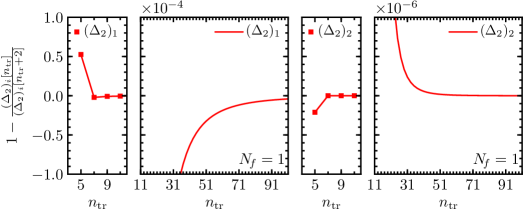
Figure 1: For the flavor-nonsinglet four-fermion operators we compute the ${n_{\mathrm{t}r}}$ and the ${n_{\mathrm{t}r}}+2$ approximation to the two $(\Delta_{2})_{i}$’s. We plot the change between two neighbouring approximations, i.e., $1-\frac{(\Delta_{2})_{i}[{n_{\mathrm{t}r}}]}{(\Delta_{2})_{i}[{n_{\mathrm{t}r}}+2]}$, as function of the truncation point ${n_{\mathrm{t}r}}$ for the case $N_{\!f}=1$. The left, right figure shows the truncation dependence of $(\Delta_{2})_{1}$ and $(\Delta_{2})_{2}$, respectively.

We implemented this algorithm for different values of the parameter $N_{\!f}$. Figure 1 shows how the NLO contribution to the scaling dimension $(\Delta_{2})_{i}$ relaxes as we increase the point of truncation. To demonstrate this we plot the change in the approximation of $(\Delta_{2})_{i}$ when the ${n_{\mathrm{t}r}}$ is increased by 2, i.e, $1-\tfrac{(\Delta_{2})_{i}[{n_{\mathrm{t}r}}]}{(\Delta_{2})_{i}[{n_{\mathrm{t}r}}+2]}$ , as a function of ${n_{\mathrm{t}r}}$ for the case of $N_{\!f}=1$. The behavior for larger $N_{\!f}$ is analogous. The plots show that as ${n_{\mathrm{t}r}}$ increases the solution approaches a constant value, indicating that the limit in eq. (5.17) indeed exists. In table 1 we list the values of $(\Delta_{2})_{1,2}$ for $N_{\!f}=1,\dots,10$ for a truncation point so large that the significant digits displayed are stable. For comparison, we also show the LO values $(\Delta_{1})_{1,2}$. Note, that with this choice of basis, i.e., $a_{n}=b_{n}=0$, diagonalizing only the physical–physical block in the flavor scheme, i.e., not accounting for evanescent operators, amounts to a sizable numerical error. For instance, for $N_{\!f}=1$ we find that $1-\frac{(\Delta_{2})_{i}[{n_{\mathrm{t}r}}=5]}{(\Delta_{2})_{i}}=51\%,-21\%$ for $i=1,2$, respectively.

$\boldsymbol{N_{\!f}}$ $1$ $2$ $3$ $4$ $5$ $6$ $7$ $8$ $9$ $10$ $\boldsymbol{(\Delta_{1})_{1}}$ $-9.00$ $-4.50$ $-3.00$ $-2.25$ $-1.80$ $-1.50$ $-1.29$ $-1.12$ $-1.00$ $-0.900$ $\boldsymbol{(\Delta_{2})_{1}}$ $35.6$ $8.53$ $3.63$ $1.95$ $1.19$ $0.782$ $0.544$ $0.393$ $0.292$ $0.221$ $\boldsymbol{(\Delta_{1})_{2}}$ $9.00$ $4.50$ $3.00$ $2.25$ $1.80$ $1.50$ $1.29$ $1.12$ $1.00$ $0.900$ $\boldsymbol{(\Delta_{2})_{2}}$ $-101$ $-29.3$ $-14.9$ $-9.40$ $-6.67$ $-5.09$ $-4.08$ $-3.38$ $-2.87$ $-2.49$

Table 1: Three significant digits of the one-loop, $(\Delta_{1})_{i}$, and the two-loop, $(\Delta_{2})_{i}$, contributions to the scaling dimension of the flavor-nonsinglet operators for various cases of $N_{\!f}$. To obtain the two-loop $(\Delta_{2})_{i}$ values we implemented the algorithm to include the effect of evanescent operators. Higher truncation of the procedure does not affect the three significant digits displayed here.

In appendix D we also include the arbitrary coefficients $a_{n}$ and $b_{n}$ of eq. (5.3). While the truncated solutions depend linearly on $a_{n}$ and $b_{n}$, we show that the coefficients of the terms proportional to $a_{n}$ and $b_{n}$ decrease to zero as we increase ${n_{\mathrm{t}r}}$. This is an important check that the answer we obtain is indeed a physical observable, independent of the choice of basis and renormalization scheme.

5.2 Flavor-singlet operators

We use the same approach to compute the NLO scaling dimensions for the flavor-singlet four-fermion operators for which $T^{ac}_{bd}=\delta^{a}_{b}\delta^{c}_{d}$, i.e.,

$$\mathscr{Q}_{1} =(\overline{\Psi}_{a}\gamma_{\mu}\Psi^{a})^{2}~{},$$ (5.18)

$$\mathscr{Q}_{3} =(\overline{\Psi}_{a}\Gamma^{3}_{\mu_{1}\mu_{2}\mu_{3}}\Psi^{a})^{2}\,.$$ (5.19)

Since the traces of $T^{ac}_{bd}$ are not zero, there are more diagrams contributing. As a result the ADM is not the same as in the flavor-nonsinglet case, and there more non-zero entries of the mixing matrix compared to the flavor-nonsinglet case. In particular, while the flavor-nonsinglet case had a single non-zero $\mathscr{E}\mathscr{Q}$ entry at NLO (see eq. (5.7)), there are infinitely many non-zero entries in the flavor-singlet case. In addition to the $(5,3)$ entry of eq. (5.7), we find that

$$(\gamma_{2}^{*})_{n1}=\frac{24}{N_{\!f}}(-1)^{\frac{n(n-1)}{2}}(n-2)(n-5)!~{},$$ (5.20)

where $n$ runs over all odd positive integers $\geq 5$. In terms of the general flavor tensor, this contribution is proportional to $T^{ab}_{bd}$, which explains why it vanishes in the flavor-nonsinglet case. To compute eq. (5.20) we use the identity [35]

$$\Gamma^{n}_{\mu_{1}\dots\mu_{n}}\gamma^{\nu}\Gamma^{n\,\mu_{1}\dots\mu_{n}} \overset{\phantom{\epsilon\to 0}}{=}(-1)^{\frac{n(n-1)}{2}}\frac{\Gamma(d)}{\Gamma(d-n+1)}(-1)^{n}(d-2n)\,\gamma^{\nu}$$

$$\overset{\epsilon\to 0}{=}-(-1)^{\frac{n(n-1)}{2}}24(n-2)(n-5)!\,\epsilon\,\gamma^{\nu}+{\cal O}(\epsilon^{2})~{}.$$ (5.21)

We collect the results for the ADM in appendix C. The LO ADM at the fixed point then follows from them; it reads

$$(\gamma_{1}^{*})_{nm}=\frac{3}{2N_{\!f}}\times\left\{\begin{array}[]{cl}8\delta_{n3}+n(n-1)(n-5)(n-6)&\text{for}\quad m=n-2\\ \frac{4}{3}(2N_{\!f}+1)\delta_{n1}-2(n-1)(n-3)&\text{for}\quad m=n\\ 1&\text{for}\quad m=n+2\\ 0&\text{otherwise}\end{array}\right.$$ (5.22)

and the physical–physical block of the NLO ADM at the fixed point is

$$(\gamma_{2}^{*})_{\mathscr{Q}\mathscr{Q}}=-\frac{1}{24N_{\!f}^{2}}\begin{bmatrix}2383+224N_{\!f}&375+18N_{\!f}\\ -1212-2568N_{\!f}&-1485-360N_{\!f}\end{bmatrix}~{}.$$ (5.23)

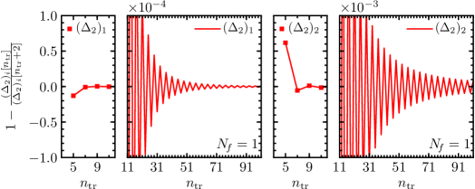
Figure 2: For the flavor-singlet four-fermion operators we compute the ${n_{\mathrm{t}r}}$ and the ${n_{\mathrm{t}r}}+2$ approximation to the two $(\Delta_{2})_{i}$’s. We plot the change between two neighbouring approximations, i.e., $1-\frac{(\Delta_{2})_{i}[{n_{\mathrm{t}r}}]}{(\Delta_{2})_{i}[{n_{\mathrm{t}r}}+2]}$, as function of the truncation point ${n_{\mathrm{t}r}}$ for the case $N_{\!f}=1$. The left, right figure shows the truncation dependence of $(\Delta_{2})_{1}$ and $(\Delta_{2})_{2}$, respectively.

Analogously to the previous section we perform a change of scheme and fix the finite renormalization constants by requiring that the $\mathscr{E}\mathscr{Q}$ entries of $\gamma_{2}^{*}$ vanish in the new scheme. This requirement defines a recurrence relation analogous to the one of eqs. (5.9) and (5.10), which we solve with the same algorithm as above. Note that the presence of infinitely many off-diagonal entries does not change qualitatively the procedure. Also in this case we see that the solution converges to a constant as we increase the size of the truncation, as shown in figure 2, which is the analogue of figure 1 for the flavor-singlet case. We list the values of the ${\cal O}(\epsilon^{2})$ corrections, $(\Delta_{2})_{i}$, for $N_{\!f}=1,\dots,10$ in table 2. For comparison we also list the LO values, $(\Delta_{1})_{i}$, for the respective $N_{\!f}$ values. Note that with this choice of basis, i.e., $a_{n}=b_{n}=0$, diagonalizing only the physical–physical block, amounts for $N_{\!f}=1$ to a numerical error of $1-\frac{(\Delta_{2})_{i}[{n_{\mathrm{t}r}}=5]}{(\Delta_{2})_{i}}=-14\%,140\%$ for $i=1,2$, respectively. Also for this flavor-singlet case, we demonstrate in appendix D the independence of the scaling dimension on the parameters $a_{n}$ and $b_{n}$ from eq. (5.3).

$\boldsymbol{N_{\!f}}$ $1$ $2$ $3$ $4$ $5$ $6$ $7$ $8$ $9$ $10$ $\boldsymbol{(\Delta_{1})_{1}}$ $-7.39$ $-3.07$ $-1.72$ $-1.10$ $-0.766$ $-0.562$ $-0.429$ $-0.337$ $-0.272$ $-0.224$ $\boldsymbol{(\Delta_{2})_{1}}$ $46.1$ $14.1$ $7.43$ $4.84$ $3.51$ $2.73$ $2.21$ $1.86$ $1.59$ $1.39$ $\boldsymbol{(\Delta_{1})_{2}}$ $13.4$ $8.07$ $6.39$ $5.60$ $5.17$ $4.90$ $4.71$ $4.59$ $4.49$ $4.42$ $\boldsymbol{(\Delta_{2})_{2}}$ $-84.0$ $-23.5$ $-11.6$ $-7.12$ $-4.94$ $-3.70$ $-2.91$ $-2.37$ $-1.99$ $-1.70$

Table 2: Three significant digits of the one-loop, $(\Delta_{1})_{i}$, and the two-loop, $(\Delta_{2})_{i}$, contributions to the scaling dimension of the flavor-singlet operators for various cases of $N_{\!f}$. To obtain the two-loop $(\Delta_{2})_{i}$ values we implemented the algorithm to include the effect of evanescent operators. Higher truncation of the procedure does not affect the three significant digits displayed here.

6 Conclusions and future directions

We studied operator mixing involving an infinite family of evanescent operators in a $d$-dimensional theory, showing how to extract the scaling dimensions at the fixed point beyond leading order in $\epsilon$. At ${\cal O}(\epsilon^{2})$, the scaling dimension is sensitive to the one-loop mixing of the whole tower of operators. We demonstrated the independence of scaling dimensions on the choice of basis and renormalization scheme. We explicitly computed the ${\cal O}(\epsilon^{2})$ corrections in the example of four-fermion operators in QED.

In light of our findings, it would be interesting to revisit the ${\cal O}(\epsilon^{4})$ computation of the scaling dimension of the four-fermion interaction in the Gross–Neveu model from ref. [15]. Since in this case the evanescent operators are first generated at three loops, we expect the whole evanescent tower to affect the ${\cal O}(\epsilon^{4})$ term of the scaling dimension.

In the present work we only applied our method to extract the first few eigenvalues of the ADM, whose eigenoperators approach the physical operators for $\epsilon\to 0$. The same procedure can also be applied to obtain additional eigenvalues. It would be interesting to study whether the additional eigenoperators also approach the physical operators as $\epsilon\to 0$, or whether they are evanescent. The first case would mean that there exist multiple continuations of the physical operators to non-integer dimension and correspondingly multiple functions that continue their scaling dimensions. Another aspect that we have not addressed in this work and that deserves further investigation is the loss of unitarity of the $d$-dimensional CFT. In analogy to refs. [8, 9], we expect that among the tower of evanescent operators one may find states of negative norm, and operators of complex scaling dimensions.

Acknowledgements: we thank Joachim Brod, Martin Gorbahn, John Gracey, Zohar Komargodski, Giampiero Paffuti, and David Stone for their interest and the many helpful discussions. We are also indebted to the Weizmann Institute of Science, in which this research began. Research at Perimeter Institute is supported by the Government of Canada through Industry Canada and by the Province of Ontario through the Ministry of Research & Innovation.

Appendix A RG equations and scaling dimensions in $\boldsymbol{d=4-2\epsilon}$

In this appendix we review how to derive the expression for the scaling dimensions in terms of the ADM at the fixed point. This is usually done by solving the RG equation for the renormalized two-point function [32, 33, 34]. The present derivation will emphasize the viewpoint that the renormalization constants are resumming the leading contributions for small $\epsilon$. We use this to take the IR limit of the “bare” two-point function.

Consider a set of operators $(\mathscr{O}_{0})_{i}$ that mix under the RG. We use the subscript “$0$” to distinguish them from the renormalized operators, whose correlators have a smooth $\epsilon\to 0$ limit. Recall that in $d=4-2\epsilon$ we have a dimensionful coupling $\alpha_{0}$ of dimension $2\epsilon$. When $|k|^{2\epsilon}\ll\alpha_{0}$ with $k$ the momentum of the operator insertion, we can expand the bare two-point function as

$$\langle(\mathscr{O}_{0})_{i}(-k)(\mathscr{O}_{0})_{j}(k)\rangle=|k|^{2\Delta_{{\mathrm{U}V}}-d}\sum_{L=0}^{\infty}(\alpha_{0}|k|^{-2\epsilon})^{L}\sum_{M=-L}^{\infty}\rho_{0\,ij}^{(L,-M)}\epsilon^{M}~{}.$$ (A.1)

We are interested in the IR limit of this two-point function, namely the limit of large $\alpha_{0}|k|^{-2\epsilon}$. We keep $\epsilon\ll 1$ and fixed.

To constrain the two-point function we use input from the renormalized theory. More precisely, we use the fact that there exist renormalized variables $\alpha$ and $\mathscr{O}_{j}$ defined as

$$\alpha_{0} =Z_{\alpha}\alpha(\mu)\mu^{2\epsilon}~{},$$ (A.2)

$$(\mathscr{O}_{0})_{i} =\sum_{j}(\mathcal{Z}^{-1})_{i}^{~{}j}\mathscr{O}_{j}~{},$$ (A.3)

such that the renormalized two-point function, as a function of the renormalized coupling, has a smooth $\epsilon\to 0$ limit. The renormalized two-point function also has a perturbative expansion, i.e.,

$$\langle\mathscr{O}_{i}(-k)\mathscr{O}_{j}(k)\rangle=|k|^{2\Delta_{{\mathrm{U}V}}-d}\sum_{L=0}^{\infty}\alpha(\mu)^{L}\sum_{M=0}^{L}\rho^{(L,M)}_{ij}\log(k^{2}/\mu^{2})^{M}~{},$$ (A.4)

where $\alpha(\mu)$ is the renormalized coupling, and $\mu$ the arbitrary renormalization scale. The negative powers of $\epsilon$ in eq. (A.1) were chosen to match the powers of $\log(k^{2}/\mu^{2})$ in eq. (A.4) as we take $\epsilon\to 0$.

From eqs. (2.9) and (2.10) we have that

$$-Z_{\alpha}\frac{\beta(\alpha,\epsilon)}{\alpha}=\frac{d\,Z_{\alpha}}{d\log\mu} =(\partial_{\alpha}Z_{\alpha})(-2\epsilon\alpha+\beta(\alpha,\epsilon))\,,$$ (A.5)

$$-\mathcal{Z}_{i}^{~{}k}\gamma(\alpha,\epsilon)_{k}^{~{}j}=\frac{d\,\mathcal{Z}_{i}^{~{}j}}{d\log\mu} =(\partial_{\alpha}\mathcal{Z}_{i}^{~{}j})(-2\epsilon\alpha+\beta(\alpha,\epsilon))\,.$$ (A.6)

The solution to these equations with boundary conditions $Z_{\alpha}(\alpha=0)=1$, $\mathcal{Z}_{i}^{~{}j}(\alpha=0)=\mathbb{1}$ is

$$Z_{\alpha}(\alpha,\epsilon) =\exp\left(\int_{0}^{\alpha}d\alpha^{\prime}\,\frac{\beta(\alpha^{\prime},\epsilon)/\alpha^{\prime}}{2\epsilon\alpha^{\prime}-\beta(\alpha^{\prime},\epsilon)}\right)~{},$$ (A.7)

$$\mathcal{Z}(\alpha,\epsilon) =\mathrm{\bar{P}exp}\left(\int_{0}^{\alpha}d\alpha^{\prime}\,\frac{\gamma(\alpha^{\prime},\epsilon)}{2\epsilon\alpha^{\prime}-\beta(\alpha^{\prime},\epsilon)}\right)~{},$$ (A.8)

up to the addition of functions of the variable $\epsilon$ alone, which are not important in what follows. $\mathrm{\bar{P}}$ denotes anti-path ordering. Note that the integral in the exponent of eq. (A.7) is finite near the lower end $\alpha=0$, because in this region $\beta(\alpha,\epsilon)=-2\beta^{(1,0)}\alpha^{2}+{\cal O}(\alpha^{3})$.

The dimensionless parameter that becomes large in the IR limit is

$$\alpha_{0}|k|^{-2\epsilon}=Z_{\alpha}\alpha(\mu)\left(\tfrac{\mu}{|k|}\right)^{2\epsilon}~{}.$$ (A.9)

Therefore, taking this IR limit while maintaining $\mu=|k|$, implies that on the right-hand side $Z_{\alpha}\alpha(\mu)$ must become large. As $\alpha$ grows continuously on the positive real axis, starting from the UV value $\alpha=0$, the constant $Z_{\alpha}$ can become large if $\alpha$ approaches a pole of the integrand of eq. (A.7), i.e., a non-trivial fixed point $\alpha^{*}$. Close to the solution we expand $-2\epsilon\alpha+\beta(\alpha,\epsilon)\sim C(\alpha-\alpha^{*})$. Substituting this in the integral, we find the leading behavior of $\alpha_{0}|k|^{-2\epsilon}$ as $\alpha$ approaches the fixed point

$$\alpha_{0}|k|^{-2\epsilon}\sim\alpha^{*}|\alpha-\alpha^{*}|^{-\frac{2\epsilon}{C}}~{}.$$ (A.10)

Given that $\epsilon\ll 1$ we can see perturbatively that the fixed point exists when $\beta^{(1,0)}<0$ and that $C>0$. The latter inequality ensures that indeed $\alpha_{0}|k|^{-2\epsilon}$ grows as we approach the fixed point.

Similarly to $Z_{\alpha}$, eq. (A.8) implies that as $\alpha\to\alpha^{*}$ the leading behavior of $\mathcal{Z}_{i}^{~{}j}$ is

$$\mathcal{Z}_{i}^{~{}j}\sim|\alpha-\alpha^{*}|^{-\tfrac{\gamma(\alpha^{*},\epsilon)}{C}}~{}.$$ (A.11)

Using eq. (A.10), we find that in the IR limit $\mathcal{Z}_{i}^{~{}j}$ becomes a power-law in $|k|$, namely

$$\mathcal{Z}_{i}^{~{}j}\sim\left(\frac{|k|}{\Lambda}\right)^{-\gamma(\alpha^{*},\epsilon)}~{},$$ (A.12)

where we introduced the crossover scale $\Lambda$, whose leading behavior as a function of $\epsilon$ for $\epsilon\ll 1$ is

$$\Lambda\sim\left(-\beta^{(1,0)}\frac{\alpha_{0}}{\epsilon}\right)^{\frac{1}{2\epsilon}}~{}.$$ (A.13)

Recalling that

$$\langle(\mathscr{O}_{0})_{i}(-k)(\mathscr{O}_{0})_{j}(k)\rangle=(\mathcal{Z}^{-1})_{i}^{~{}k}(\mathcal{Z}^{-1})_{j}^{~{}l}\langle\mathscr{O}_{k}(-k)\mathscr{O}_{l}(k)\rangle~{},$$ (A.14)

and using eqs. (A.12) and (A.4) for $\mu=|k|$ we see that in the IR limit a new scaling behavior emerges, i.e.,

$$\langle(\mathscr{O}_{0})_{i}(-k)(\mathscr{O}_{0})_{j}(k)\rangle\underset{|k|\ll\Lambda}{\sim}|k|^{2(\Delta_{\mathrm{U}V}+\gamma(\alpha^{*},\epsilon))-d}\,,$$ (A.15)

corresponding to the IR scaling dimension $\Delta_{{\mathrm{I}R}}=\Delta_{{\mathrm{U}V}}+\gamma(\alpha^{*},\epsilon)$. We also see that more precisely the crossover to the IR scaling happens when $|k|\sim\Lambda$, with $\Lambda$ given in eq. (A.13). As observed in Ref. [16], $\Lambda$ is exponentially enhanced for $\epsilon\ll 1$ compared to the naive crossover scale $\alpha_{0}^{\frac{1}{2\epsilon}}$.

Appendix B Beta functions and anomalous dimensions

In this appendix we collect:

1. the one- and two-loop formulas for the beta function and ADM from eqs. (2.9) and (2.10), respectively. In terms of the renormalization-constant expansions from eqs. (2.3) and (2.4) they read

   $$\beta^{(1,0)} =-Z_{\alpha}^{(1,1)}~{},\qquad\beta^{(1,-1)}=-Z_{\alpha}^{(1,0)}~{},$$

   $$\beta^{(2,0)} =-2Z_{\alpha}^{(2,1)}+4Z_{\alpha}^{(1,0)}Z_{\alpha}^{(1,1)}~{},$$ (B.1)

   $$\gamma^{(1,0)} =2\mathcal{Z}^{(1,1)}~{},\qquad\gamma^{(1,-1)}=2\mathcal{Z}^{(1,0)}~{},$$

   $$\gamma^{(2,0)} =4\mathcal{Z}^{(2,1)}-2\mathcal{Z}^{(1,1)}\mathcal{Z}^{(1,0)}-2\mathcal{Z}^{(1,0)}\mathcal{Z}^{(1,1)}+2\beta^{(1,0)}\mathcal{Z}^{(1,0)}+2\beta^{(1,-1)}\mathcal{Z}^{(1,1)}~{}.$$ (B.2)

2. the relations between the one- and two-loop beta function and ADM in two different, mass-independent schemes distinguished by the superscript “$\widetilde{\phantom{a}}$”. Substituting the expansion of eqs. (2.9) and (2.11) in eq. (3.5) we find that

   $$\tilde{\beta}^{(1,0)} =\beta^{(1,0)}~{}, \tilde{\beta}^{(1,-1)} =\beta^{(1,-1)}+Z^{(1,0)}-\tilde{Z}^{(1,0)}~{},$$

   $$\tilde{\beta}^{(2,0)} =\beta^{(2,0)}~{}, \tilde{\beta}^{(2,-1)} =\beta^{(2,-1)}+2\left(Z^{(2,0)}-\tilde{Z}^{(2,0)}-(Z^{(1,0)})^{2}+(\tilde{Z}^{(1,0)})^{2}\right)~{}.$$ (B.3)

   Similarly, the expansion of eqs. (2.10) and (2.12) in eq. (3) leads to

   $$\tilde{\gamma}^{(1,0)} =\gamma^{(1,0)}~{},\qquad\quad\tilde{\gamma}^{(1,-1)}=\gamma^{(1,-1)}-2\left(\mathcal{Z}^{(1,0)}-\tilde{\mathcal{Z}}^{(1,0)}\right)$$ (B.4)

   $$\tilde{\gamma}^{(2,0)} =\gamma^{(2,0)}+\left[\gamma^{(1,0)},\mathcal{Z}^{(1,0)}-\tilde{\mathcal{Z}}^{(1,0)}\right]-2\beta^{(1,0)}\left(\mathcal{Z}^{(1,0)}-\tilde{\mathcal{Z}}^{(1,0)}\right)~{}.$$ (B.5)

Appendix C Anomalous dimensions of four-fermion operators in QED

C.1 Flavor-nonsinglet operators

The results for the one-loop anomalous dimension, and the one-loop finite renormalization in the flavor scheme can be found in ref. [11]. Including also the dependence on $a_{n},\,b_{n}$ the result is

$$\gamma^{(1,0)}_{nm} =\left\{\begin{array}[]{cl}2n(n-1)(n-5)(n-6)&\text{for}\quad m=n-2\\ -4(n-1)(n-3)&\text{for}\quad m=n\\ 2&\text{for}\quad m=n+2\\ 0&\text{otherwise\,,}\\ \end{array}\right.$$ (C.5)

$$\gamma^{(1,-1)}_{nm} =\left\{\begin{array}[]{ll}-2n(n-1)(n-5)(n-6)a_{n-2}\\ \quad+4(n-1)(n-3)a_{n}-2a_{n+2}+72b_{n}&\text{for}~{}m=1,\,n\geq 5\\[10.00002pt] -80\delta_{n5}\\ \quad-2n(n-1)(n-5)(n-6)b_{n-2}\\ \qquad+4(n-1)(n-3)b_{n}-2b_{n+2}+2a_{n}&\text{for}~{}m=3,\,n\geq 5\\[10.00002pt] \hskip 70.0001pt0&\text{otherwise\,.}\end{array}\right.$$ (C.12)

We computed also the $(\mathscr{Q}_{1},\mathscr{Q}_{3})$ entries of the two-loop anomalous dimension in the same scheme, finding

$$\begin{split}\gamma^{(2,0)}_{\mathscr{Q}\mathscr{Q}}&=\left[\begin{array}[]{cc}-162&-28-\frac{4}{9}N_{\!f}\\ 144-176N_{\!f}&78-\frac{64}{3}N_{\!f}\end{array}\right]+\\ &+a_{5}\left[\begin{array}[]{cc}-2&0\\ -\frac{8}{3}N_{\!f}&2\\ \end{array}\right]+b_{5}\left[\begin{array}[]{cc}0&-2\\ 72&-\frac{8}{3}N_{\!f}\\ \end{array}\right]\,.\end{split}$$ (C.13)

Moreover, as explained in section 4, in this scheme $\gamma^{(1,0)}_{\mathscr{E}\mathscr{Q}}=\gamma^{(2,0)}_{\mathscr{E}\mathscr{Q}}=0$.

Using eqs. (2.17) and (2.18) we obtain the ADM at the fixed point

$$(\gamma_{1}^{*})_{nm} =\frac{3}{2N_{\!f}}\times\left\{\begin{array}[]{cl}n(n-1)(n-5)(n-6)&\text{for}\quad m=n-2\\ -2(n-1)(n-3)&\text{for}\quad m=n\\ 1&\text{for}\quad m=n+2\\ 0&\text{otherwise\,.}\end{array}\right.$$ (C.18)

$$(\gamma_{2}^{*})_{nm} =\left\{\begin{array}[]{ll}-\frac{1}{8N_{\!f}^{2}}\begin{bmatrix}729&153+2N_{\!f}\\ 324+792N_{\!f}&-351+96N_{\!f}\end{bmatrix}&\\ +\frac{3}{8N_{\!f}^{2}}a_{5}\begin{bmatrix}-3&0\\ -4N_{\!f}&3\end{bmatrix}+\frac{3}{8N_{\!f}^{2}}b_{5}\begin{bmatrix}0&-3\\ 108&-4N_{\!f}\end{bmatrix}&\text{for}\quad n,m=1,3\,,\\[20.00003pt] \frac{3}{2N_{\!f}}\left(-n(n-1)(n-5)(n-6)a_{n-2}\right.\\ \left.\qquad+2(n-1)(n-3)a_{n}-a_{n+2}+36b_{n}\right)&\text{for}~{}m=1,\,n\geq 5~{},\\[10.00002pt] -\frac{60}{N_{\!f}}\delta_{n5}\\ \quad+\frac{3}{2N_{\!f}}\left(-n(n-1)(n-5)(n-6)b_{n-2}\right.\\ \qquad\left.+2(n-1)(n-3)b_{n}-b_{n+2}+a_{n}\right)&\text{for}~{}m=3,\,n\geq 5~{},\\[10.00002pt] \hskip 50.00008pt\text{not required}&\text{otherwise\,.}\end{array}\right.$$ (C.27)

C.2 Flavor-singlet operators

The one-loop anomalous dimension in the physical sector can be found in refs. [36, 16]. The one-loop $\mathscr{E}\mathscr{Q}$ finite terms and the two-loop $\mathscr{Q}\mathscr{Q}$ ADM in the flavor scheme are computed in ref. [27]. The results are

$$\gamma^{(1,0)}_{nm} =\left\{\begin{array}[]{cl}16\delta_{n3}+2n(n-1)(n-5)(n-6)&\text{for}\quad m=n-2\\ \frac{8}{3}(2N_{\!f}+1)\delta_{n1}-4(n-1)(n-3)&\text{for}\quad m=n\\ 2&\text{for}\quad m=n+2\\ 0&\text{otherwise\,,}\\ \end{array}\right.$$ (C.32)

$$\gamma^{(1,-1)}_{nm} =\left\{\begin{array}[]{ll}32(-1)^{\frac{n(n-1)}{2}}(n-2)(n-5)!\\ \quad-2n(n-1)(n-5)(n-6)a_{n-2}\\ \qquad+\left(\frac{8}{3}(2N_{\!f}+1)+4(n-1)(n-3)\right)a_{n}\\ \qquad\quad-2a_{n+2}+88b_{n}&\text{for}~{}m=1,\,n\geq 5\\[10.00002pt] -80\delta_{n5}\\ \quad-2n(n-1)(n-5)(n-6)b_{n-2}\\ \qquad+4(n-1)(n-3)b_{n}-2b_{n+2}+2a_{n}&\text{for}~{}m=3,\,n\geq 5\\[10.00002pt] \hskip 70.0001pt0&\text{otherwise\,,}\end{array}\right.$$ (C.41)

and

$$\begin{split}\gamma^{(2,0)}_{\mathscr{Q}\mathscr{Q}}&=\left[\begin{array}[]{cc}-\frac{2}{27}(2275+8N_{\!f})&-\frac{4}{9}(49+3N_{\!f})\\ \frac{16}{9}(199+107N_{\!f})&110+\frac{80N_{\!f}}{3}\end{array}\right]+\\ &+a_{5}\left[\begin{array}[]{cc}-2&0\\ \frac{8}{3}(1+N_{\!f})&2\\ \end{array}\right]+b_{5}\left[\begin{array}[]{cc}0&-2\\ 88&-\frac{8}{3}N_{\!f}\\ \end{array}\right]~{}.\end{split}$$ (C.42)

Also in this case $\gamma^{(1,0)}_{\mathscr{E}\mathscr{Q}}=\gamma^{(2,0)}_{\mathscr{E}\mathscr{Q}}=0$ in agreement with the general results of section 4.

Using eqs. (2.17) and (2.18) we obtain the ADM at the fixed point

$$(\gamma_{1}^{*})_{nm} =\frac{3}{2N_{\!f}}\times\left\{\begin{array}[]{cl}8\delta_{n3}+n(n-1)(n-5)(n-6)&\text{for}\quad m=n-2\\ \frac{4}{3}(2N_{\!f}+1)\delta_{n1}-2(n-1)(n-3)&\text{for}\quad m=n\\ 1&\text{for}\quad m=n+2{}\\ 0&\text{otherwise}~{},\end{array}\right.$$ (C.47)

$$(\gamma_{2}^{*})_{nm} =\left\{\begin{array}[]{ll}-\frac{1}{24N_{\!f}^{2}}\begin{bmatrix}2383+224N_{\!f}&375+18N_{\!f}\\ -1212-2568N_{\!f}&-1485-360N_{\!f}\end{bmatrix}&\\ +\frac{3}{8N_{\!f}^{2}}a_{5}\begin{bmatrix}-3&0\\ 4N_{\!f}+4&3\end{bmatrix}+\frac{3}{8N_{\!f}^{2}}b_{5}\begin{bmatrix}0&-3\\ 132&-4N_{\!f}\end{bmatrix}&\text{for}~{}n,m=1,3~{},\\[20.00003pt] \frac{24}{N_{\!f}}(-1)^{\frac{n(n-1)}{2}}(n-2)(n-5)!\\ \quad+\frac{3}{2N_{\!f}}\left(-n(n-1)(n-5)(n-6)a_{n-2}\right.\\ \qquad+\left(\frac{4}{3}(2N_{\!f}+1)+2(n-1)(n-3)\right)a_{n}\\ \qquad\quad\left.-a_{n+2}+44b_{n}\right)&\text{for}~{}m=1,\,n\geq 5~{},\\[10.00002pt] -\frac{60}{N_{\!f}}\delta_{n5}\\ \quad+\frac{3}{2N_{\!f}}\left(-n(n-1)(n-5)(n-6)b_{n-2}\right.\\ \qquad\left.+2(n-1)(n-3)b_{n}-b_{n+2}+a_{n}\right)&\text{for}~{}m=3,\,n\geq 5~{},\\[10.00002pt] \hskip 70.0001pt\text{not required}&\text{otherwise\,.}\end{array}\right.$$ (C.58)

Appendix D $\boldsymbol{a_{n}}$ and $\boldsymbol{b_{n}}$ independence

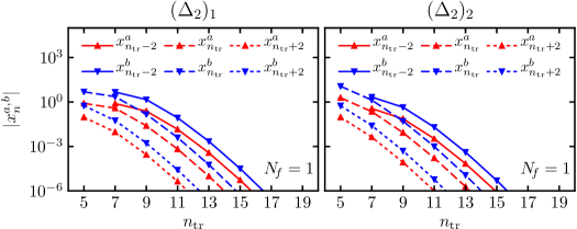
Figure 3: For the case of flavor-nonsinglet operators, we plot the coefficient of the basis-dependent parameters $a_{n}$ and $b_{n}$ in the truncated result for the NLO scaling dimension, as a function of the truncation number ${n_{\mathrm{t}r}}$, for $N_{\!f}=1$. We see that as we increase the number of evanescent operators included, the dependence drops from the observable. See eq. (D.7) for more details.

In appendix C we collected the results for the ADM for both the flavor-singlet and flavor-nonsinglet operators computed in the generic basis of eq. (5.3). We observe that both the $\mathscr{E}\mathscr{Q}$ finite one-loop mixing and the two-loop $\mathscr{Q}\mathscr{Q}$ mixing depends linearly on the coefficients $a_{n}$ and $b_{n}$. As a result, in this generic basis, the entries of $\gamma_{2}^{*}$, which we use to compute the NLO scaling dimension, also depend on $a_{n}$ and $b_{n}$. However, the parameters $a_{n}$ and $b_{n}$ are just a parametrization of our freedom to choose the basis of operators. Therefore, the observables, i.e., the scaling dimensions, cannot depend on them. In this appendix, we demonstrate using the algorithm from section 5 how this unphysical dependence indeed cancels in the observables. This has to be contrasted with the wrong procedure of naively diagonalizing the $\mathscr{Q}\mathscr{Q}$ block of the two-loop ADM in the flavor scheme, which would lead to eigenvalues that depend on $a_{n}$ and $b_{n}$.

To this end, we first generalize eqs. (5.13) and (5.14) to the case in which the basis includes $a_{n}$ and $b_{n}$. The generalizations for the two considered cases follow:
Flavor-nonsinglet case:

$$(\Delta_{2})_{1} =\frac{3}{32N_{\!f}^{2}}\biggl{(}156+32N_{\!f}-\left(10-\frac{4}{3}N_{\!f}\right)a_{5}+a_{7}+(60-8N_{\!f})b_{5}-6b_{7}$$

$$\hskip 220.00034pt+\tilde{\mathcal{Z}}^{(1,0)}_{51}-6\tilde{\mathcal{Z}}^{(1,0)}_{53}\biggr{)}~{},$$ (D.1)

$$(\Delta_{2})_{2} =\frac{3}{32N_{\!f}^{2}}\biggl{(}-1140-160N_{\!f}+\left(22-\frac{4}{3}N_{\!f}\right)a_{5}-a_{7}+(132-8N_{\!f})b_{5}-6b_{7}$$

$$\hskip 220.00034pt-\tilde{\mathcal{Z}}^{(1,0)}_{51}-6\tilde{\mathcal{Z}}^{(1,0)}_{53}\biggr{)}\,.$$ (D.2)

Flavor-singlet case:

$$(\Delta_{2})_{1}=\frac{1}{192N_{\!f}^{2}\kappa}\biggl{(}+ 47552-7912\kappa+(6992+544\kappa)N_{\!f}+2336N_{\!f}^{2}$$

$$- (1350-108\kappa)a_{5}$$

$$+ 81a_{7}$$

$$- (2700-1728\kappa-(1656-144\kappa)N_{\!f}+144N_{\!f}^{2})b_{5}$$

$$- (54+108\kappa+108N_{\!f})b_{7}$$

$$+ 81\tilde{\mathcal{Z}}^{(1,0)}_{51}-(54+108\kappa+108N_{\!f})\tilde{\mathcal{Z}}^{(1,0)}_{53}\biggr{)}\,,$$ (D.3)

$$(\Delta_{2})_{2}=\frac{1}{192N_{\!f}^{2}\kappa}\biggl{(}- 47552-7912\kappa+(-6992+544\kappa)N_{\!f}-2336N_{\!f}^{2}$$

$$+ (1350+108\kappa)a_{5}$$

$$- 81a_{7}$$

$$+ (2700+1728\kappa-(1656+144\kappa)N_{\!f}+144N_{\!f}^{2})b_{5}$$

$$+ (54-108\kappa+108N_{\!f})b_{7}$$

$$- 81\tilde{\mathcal{Z}}^{(1,0)}_{51}+(54-108\kappa+108N_{\!f})\tilde{\mathcal{Z}}^{(1,0)}_{53}\biggr{)}\,,$$ (D.4)

where we introduced

$$\kappa\equiv\sqrt{N_{\!f}^{2}+N_{\!f}+25}\,.$$ (D.5)

We see that in both cases $(\Delta_{2})_{i}$ depend linearly on $a_{n}$, $b_{n}$ with $n=5,7$ and on the finite renormalization constants $\tilde{\mathcal{Z}}^{(1,0)}_{51}$ and $\tilde{\mathcal{Z}}^{(1,0)}_{53}$. By setting the $\mathscr{E}\mathscr{Q}$ entries of $\tilde{\gamma}_{2}^{*}$ in eqs. (C.27) and (C.58) to zero, we obtain a generalization of the recurrence relation in eqs. (5.9) and (5.10) for $\tilde{\mathcal{Z}}^{(1,0)}$, with additional terms linear in $a_{n}$, $b_{n}$. After solving the truncated system of equations with $n<{n_{\mathrm{t}r}}$ and substituting back the solution for $\tilde{\mathcal{Z}}^{(1,0)}_{51}$ and $\tilde{\mathcal{Z}}^{(1,0)}_{53}$ in terms of $\tilde{\mathcal{Z}}^{(1,0)}_{{n_{\mathrm{t}r}}1}$ and $\tilde{\mathcal{Z}}^{(1,0)}_{{n_{\mathrm{t}r}}3}$, we find that the dependence on $a_{n}$ and $b_{n}$ for $n<{n_{\mathrm{t}r}}-2$ cancels. The ${n_{\mathrm{t}r}}$ approximation to the observable, $\Delta_{2}[{n_{\mathrm{t}r}}]$, defined by

$$\Delta_{2}=\Delta_{2}[{n_{\mathrm{t}r}}]+x^{\mathcal{Z}}_{1}[{n_{\mathrm{t}r}}]\,\tilde{\mathcal{Z}}^{(1,0)}_{{n_{\mathrm{t}r}}1}+x^{\mathcal{Z}}_{3}[{n_{\mathrm{t}r}}]\,\tilde{\mathcal{Z}}^{(1,0)}_{{n_{\mathrm{t}r}}3}~{},$$ (D.6)

depends solely on higher $a_{n}$’s and $b_{n}$’s, namely

$$\begin{split}\Delta_{2}[{n_{\mathrm{t}r}}]=\Delta_{2}[{n_{\mathrm{t}r}}]\biggl{|}_{a_{n}=b_{n}=0}+&x^{a}_{{n_{\mathrm{t}r}}-2}[{n_{\mathrm{t}r}}]\,a_{{n_{\mathrm{t}r}}-2}+x^{a}_{{n_{\mathrm{t}r}}}[{n_{\mathrm{t}r}}]\,a_{{n_{\mathrm{t}r}}}+x^{a}_{{n_{\mathrm{t}r}}+2}[{n_{\mathrm{t}r}}]\,a_{{n_{\mathrm{t}r}}+2}\\ +&x^{b}_{{n_{\mathrm{t}r}}-2}[{n_{\mathrm{t}r}}]\,b_{{n_{\mathrm{t}r}}-2}+x^{b}_{{n_{\mathrm{t}r}}}[{n_{\mathrm{t}r}}]\,b_{{n_{\mathrm{t}r}}}+x^{b}_{{n_{\mathrm{t}r}}+2}[{n_{\mathrm{t}r}}]\,b_{{n_{\mathrm{t}r}}+2}\,.\end{split}$$ (D.7)

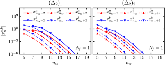
Figure 4: For the case of flavor-singlet operators, we plot the coefficient of the basis-dependent parameters $a_{n}$ and $b_{n}$ in the truncated result for the NLO scaling dimension, as a function of the truncation number ${n_{\mathrm{t}r}}$, for $N_{\!f}=1$. We see that as we increase the number of evanescent operators included, the dependence drops from the observable. See eq. (D.7) for more details.

Here, we have suppressed for brevity the subscript $i$ labelling the eigenvalue. Therefore, as a final check of the basis independence of the observable we show that the coefficients of the terms proportional to $a_{{n_{\mathrm{t}r}}-2}$, $a_{{n_{\mathrm{t}r}}}$, $a_{{n_{\mathrm{t}r}}+2}$, $b_{{n_{\mathrm{t}r}}-2}$, $b_{{n_{\mathrm{t}r}}}$, and $b_{{n_{\mathrm{t}r}}+2}$ all relax to zero as ${n_{\mathrm{t}r}}\to\infty$, i.e., that

$$\lim_{{n_{\mathrm{t}r}}\to\infty}x^{a,b}_{{n_{\mathrm{t}r}}-2}[{n_{\mathrm{t}r}}]=0\,, \lim_{{n_{\mathrm{t}r}}\to\infty}x^{a,b}_{{n_{\mathrm{t}r}}}[{n_{\mathrm{t}r}}]=0\,, \lim_{{n_{\mathrm{t}r}}\to\infty}x^{a,b}_{{n_{\mathrm{t}r}}+2}[{n_{\mathrm{t}r}}]=0\,.$$ (D.8)

We demonstrate this in figure 3 and figure 4 for the flavor-nonsinglet and flavor-singlet case, respectively, in which we plot the absolute value of these coefficients as a function of ${n_{\mathrm{t}r}}$ for the case $N_{\!f}=1$. In both cases, we observe that even after a few steps of the algorithm the coefficients have already relaxed to small values. The behavior for larger values of $N_{\!f}$ is analogous.

References

- [1] K. G. Wilson and M. E. Fisher, Critical exponents in 3.99 dimensions, Phys. Rev. Lett. 28 (1972) 240–243.
- [2] K. G. Wilson, Quantum field theory models in less than four-dimensions, Phys. Rev. D7 (1973) 2911–2926.
- [3] S. El-Showk, M. Paulos, D. Poland, S. Rychkov, D. Simmons-Duffin, and A. Vichi, Conformal Field Theories in Fractional Dimensions, Phys. Rev. Lett. 112 (2014) 141601, [arXiv:1309.5089].
- [4] S. M. Chester, S. S. Pufu, and R. Yacoby, Bootstrapping vector models in 4 6, Phys. Rev. D91 (2015), no. 8 086014, [arXiv:1412.7746].
- [5] N. Bobev, S. El-Showk, D. Mazac, and M. F. Paulos, Bootstrapping SCFTs with Four Supercharges, arXiv:1503.02081.
- [6] S. M. Chester, S. Giombi, L. V. Iliesiu, I. R. Klebanov, S. S. Pufu, and R. Yacoby, Accidental Symmetries and the Conformal Bootstrap, JHEP 01 (2016) 110, [arXiv:1507.04424].
- [7] S. M. Chester, L. V. Iliesiu, S. S. Pufu, and R. Yacoby, Bootstrapping Vector Models with Four Supercharges in , JHEP 05 (2016) 103, [arXiv:1511.07552].
- [8] M. Hogervorst, S. Rychkov, and B. C. van Rees, Truncated conformal space approach in d dimensions: A cheap alternative to lattice field theory?, Phys. Rev. D91 (2015) 025005, [arXiv:1409.1581].
- [9] M. Hogervorst, S. Rychkov, and B. C. van Rees, Unitarity violation at the Wilson-Fisher fixed point in 4- dimensions, Phys. Rev. D93 (2016), no. 12 125025, [arXiv:1512.00013].
- [10] A. J. Buras and P. H. Weisz, QCD Nonleading Corrections to Weak Decays in Dimensional Regularization and ’t Hooft-Veltman Schemes, Nucl. Phys. B333 (1990) 66.
- [11] M. J. Dugan and B. Grinstein, On the vanishing of evanescent operators, Phys. Lett. B256 (1991) 239–244.
- [12] A. Bondi, G. Curci, G. Paffuti, and P. Rossi, Ultraviolet Properties of the Generalized Thirring Model With U() Symmetry, Phys. Lett. B216 (1989) 345–348.
- [13] A. Bondi, G. Curci, G. Paffuti, and P. Rossi, Metric and Central Charge in the Perturbative Approach to Two-dimensional Fermionic Models, Annals Phys. 199 (1990) 268.
- [14] S. Herrlich and U. Nierste, Evanescent operators, scheme dependences and double insertions, Nucl. Phys. B455 (1995) 39–58, [hep-ph/9412375].
- [15] J. A. Gracey, T. Luthe, and Y. Schroder, Four loop renormalization of the Gross-Neveu model, Phys. Rev. D94 (2016), no. 12 125028, [arXiv:1609.05071].
- [16] L. Di Pietro, Z. Komargodski, I. Shamir, and E. Stamou, Quantum Electrodynamics in from the Expansion, Phys. Rev. Lett. 116 (2016), no. 13 131601, [arXiv:1508.06278].
- [17] S. Giombi, I. R. Klebanov, and G. Tarnopolsky, Conformal QEDd, -Theorem and the Expansion, J. Phys. A49 (2016), no. 13 135403, [arXiv:1508.06354].
- [18] L. Fei, S. Giombi, I. R. Klebanov, and G. Tarnopolsky, Yukawa CFTs and Emergent Supersymmetry, PTEP 2016 (2016), no. 12 12C105, [arXiv:1607.05316].
- [19] K. Diab, L. Fei, S. Giombi, I. R. Klebanov, and G. Tarnopolsky, On and in the Gross-Neveu and O(N) models, J. Phys. A49 (2016), no. 40 405402, [arXiv:1601.07198].
- [20] S. Giombi, G. Tarnopolsky, and I. R. Klebanov, On and in Conformal QED, JHEP 08 (2016) 156, [arXiv:1602.01076].
- [21] S. Giombi, V. Kirilin, and E. Skvortsov, Notes on Spinning Operators in Fermionic CFT, JHEP 05 (2017) 041, [arXiv:1701.06997].
- [22] D. Dalidovich and S.-S. Lee, Perturbative non-Fermi liquids from dimensional regularization, Phys. Rev. B88 (2013) 245106, [arXiv:1307.3170].
- [23] S. Sur and S.-S. Lee, Anisotropic non-Fermi liquids, Phys. Rev. B94 (2016), no. 19 195135, [arXiv:1606.06694].
- [24] T. Senthil and R. Shankar, Fermi surfaces in general codimension and a new controlled nontrivial fixed point, Phys. Rev. Lett. 102 (Jan, 2009) 046406.
- [25] P. Lunts, A. Schlief, and S.-S. Lee, Emergence of a control parameter for the antiferromagnetic quantum critical metal, Phys. Rev. B95 (2017), no. 24 245109.
- [26] L. Janssen and Y.-C. He, Critical behavior of the QED3-Gross-Neveu model: duality and deconfined criticality, arXiv:1708.02256.
- [27] L. Di Pietro and E. Stamou, Scaling dimensions in QED3 from the -expansion.
- [28] J. C. Collins, Renormalization, vol. 26 of Cambridge Monographs on Mathematical Physics. Cambridge University Press, Cambridge, 1986.
- [29] C. Behan, L. Rastelli, S. Rychkov, and B. Zan, A scaling theory for the long-range to short-range crossover and an infrared duality, arXiv:1703.05325.
- [30] A. N. Vasil’ev, The field theoretic renormalization group in critical behavior theory and stochastic dynamics. 2004.
- [31] W. A. Bardeen, A. J. Buras, D. W. Duke, and T. Muta, Deep Inelastic Scattering Beyond the Leading Order in Asymptotically Free Gauge Theories, Phys. Rev. D18 (1978) 3998.
- [32] P. K. Mitter, Callan-symanzik equations and epsilon expansions, Phys. Rev. D7 (1973) 2927–2942.
- [33] E. Brezin, J. C. Le Guillou, and J. Zinn-Justin, Approach to scaling in renormalized perturbation theory, Phys. Rev. D8 (1973) 2418–2430.
- [34] E. Brezin, J. C. Le Guillou, and J. Zinn-Justin, Wilson’s theory of critical phenomena and callan-symanzik equations in 4-epsilon dimensions, Phys. Rev. D8 (1973) 434–440.
- [35] A. D. Kennedy, Clifford Algebras in Two Dimensions, J. Math. Phys. 22 (1981) 1330–1337.
- [36] M. Beneke and V. A. Smirnov, Ultraviolet renormalons in Abelian gauge theories, Nucl. Phys. B472 (1996) 529–590, [hep-ph/9510437].